Updated High-Temperature Opacities for The Dartmouth Stellar Evolution Program and their Effect on the Jao Gap Location

Abstract

The Jao Gap, a 17 percent decrease in stellar density at M${}_{G}\sim$ 10 identified in both Gaia DR2 and EDR3 data, presents a new method to probe the interior structure of stars near the fully convective transition mass. The Gap is believed to originate from convective kissing instability wherein asymmetric production of ³He causes the core convective zone of a star to periodically expand and contract and consequently the stars’ luminosity to vary. Modeling of the Gap has revealed a sensitivity in its magnitude to a population’s metallicity primarily through opacity. Thus far, models of the Jao Gap have relied on OPAL high-temperature radiative opacities. Here we present updated synthetic population models tracing the Gap location modeled with the Dartmouth stellar evolution code using the OPLIB high-temperature radiative opacities. Use of these updated opacities changes the predicted location of the Jao Gap by $\sim$0.05 mag as compared to models which use the OPAL opacities. This difference is likeley too small to be detectable in empirical data.

1 INTRODUCTION

Due to the initial mass requirements of the molecular clouds which collapse to form stars, star formation is strongly biased towards lower mass, later spectral class stars when compared to higher mass stars. Partly as a result of this bias and partly as a result of their extremely long main-sequence lifetimes, M Dwarfs make up approximately 70 percent of all stars in the galaxy. Moreover, some planet search campaigns have focused on M Dwarfs due to the relative ease of detecting small planets in their habitable zones (e.g. Nutzman & Charbonneau, 2008). M Dwarfs then represent both a key component of the galactic stellar population as well as the possible set of stars which may host habitable exoplanets. Given this key location M Dwarfs occupy in modern astronomy it is important to have a thorough understanding of their structure and evolution.

Jao et al. (2018) discovered a novel feature in the Gaia Data Release 2 (DR2) $G_{BP}-G_{RP}$ color-magnitude-diagram. Around $M_{G}=10$ there is an approximately 17 percent decrease in stellar density of the sample of stars Jao et al. (2018) considered. Subsequently, this has become known as either the Jao Gap, or Gaia M Dwarf Gap. Following the initial detection of the Gap in DR2 the Gap has also potentially been observed in 2MASS (Skrutskie et al., 2006; Jao et al., 2018); however, the significance of this detection is quite weak and it relies on the prior of the Gap’s location from Gaia data. Further, the Gap is also present in Gaia Early Data Release 3 (EDR3) (Jao & Feiden, 2021). These EDR3 and 2MASS data sets then indicate that this feature is not a bias inherent to DR2.

The Gap is generally attributed to convective instabilities in the cores of stars straddling the fully convective transition mass (0.3 - 0.35 M_⊙) (Baraffe & Chabrier, 2018). These instabilities interrupt the normal, slow, main sequence luminosity evolution of a star and result in luminosities lower than expected from the main sequence mass-luminosity relation (Jao & Feiden, 2020).

The Jao Gap, inherently a feature of M Dwarf populations, provides an enticing and unique view into the interior physics of these stars (Feiden et al., 2021). This is especially important as, unlike more massive stars, M Dwarf seismology is infeasible due to the short periods and extremely small magnitudes which both radial and low-order low-degree non-radial seismic waves are predicted to have in such low mass stars (Rodríguez-López, 2019). The Jao Gap therefore provides one of the only current methods to probe the interior physics of M Dwarfs.

Despite the early success of modeling the Gap some issues remain. Jao & Feiden (2020, 2021) identify that the Gap has a wedge shape which has not been successful reproduced by any current modeling efforts and which implies a somewhat unusual population composition of young, metal-poor stars. Further, Jao & Feiden (2020) identify substructure, an additional over density of stars, directly below the Gap, again a feature not yet fully captured by current models.

All currently published models of the Jao Gap make use of OPAL high temperature radiative opacities. Here we investigate the effect of using the more up-to-date OPLIB high temperature radiative opacities and whether these opacity tables bring models more in line with observations. In Section 2 we provide an overview of the physics believed to result in the Jao Gap, in Section 3 we review the differences between OPAL and OPLIB and describe how we update DSEP to use OPLIB opacity tables. Section 4 walks through the stellar evolution and population synthesis modeling we perform. Finally, in Section 5 we present our findings.

2 Jao Gap

A theoretical explanation for the Jao Gap (Figure 1) comes from van Saders & Pinsonneault (2012), who propose that in a star directly above the transition mass, due to asymmetric production and destruction of ³He during the proton-proton I chain (ppI), periodic luminosity variations can be induced. This process is known as convective-kissing instability. Very shortly after the zero-age main sequence such a star will briefly develop a radiative core; however, as the core temperature exceeds $7\times 10^{6}$ K, enough energy will be produced by the ppI chain that the core once again becomes convective. At this point the star exists with both a convective core and envelope, in addition to a thin, radiative layer separating the two. Subsequently, asymmetries in ppI affect the evolution of the star’s convective core.

While kissing instability has been the most widely adopted model to explain the existence of the Jao Gap, slightly different mechanisms have also been proposed. MacDonald & Gizis (2018) make use of a fully implicit stellar evolution suite which treats convective mixing as a diffusive property. MacDonald & Gizis treat convective mixing this way in order to account for a core deuterium concentration gradient proposed by Baraffe et al. (1997). Under this treatment the instability results only in a single mixing event — as opposed to periodic mixing events. Single mixing events may be more in line with observations (see section 5 for more details on how periodic mixings can effect a synthetic population) where there is only well documented evidence of a single gap. However, recent work by Jao & Feiden (2021) which identify an second under density of stars below the canonical gap, does leave the door open for the periodic mixing events.

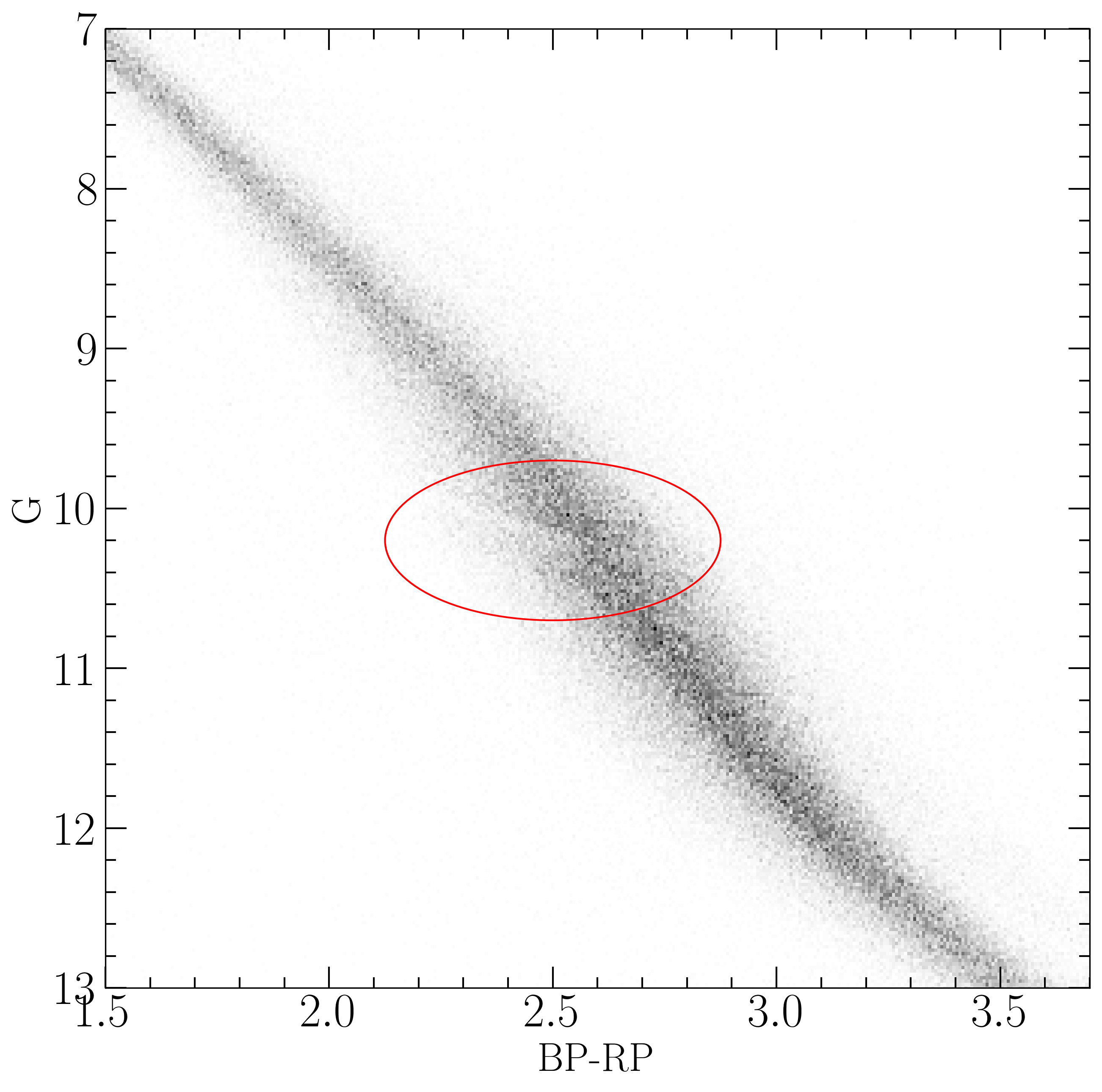
Figure 1: The Jao Gap (circled) seen in the Gaia Catalogue of Nearby Stars (Gaia Collaboration et al., 2021).

The proton-proton I chain constitutes three reactions

1. $p+p\longrightarrow d+e^{+}+\nu_{e}$

2. $p+d\longrightarrow\ ^{3}\text{He}+\gamma$

3. ${}^{3}\text{He}+^{3}\text{He}\longrightarrow\ ^{3}\text{He}+2p$

Initially, reaction 3 of ppI consumes ³He at a slower rate than it is produced by reaction 2 and as a result, the core ³He abundance and consequently the rate of reaction 3, increases with time. The core convective zone expands as more of the star becomes unstable to convection. This expansion continues until the core connects with the convective envelope. At this point convective mixing can transport material throughout the entire star and the high concentration of ³He rapidly diffuses outward, away from the core, decreasing energy generation as reaction 3 slows down. Ultimately, this leads to the convective region around the core pulling back away from the convective envelope, leaving in place the radiative transition zone, at which point ³He concentrations grow in the core until it once again expands to meet the envelope. These periodic mixing events will continue until ³He concentrations throughout the star reach an equilibrium ultimately resulting in a fully convective star. Figure 2 traces the evolution of a characteristic star within the Jao Gap’s mass range.

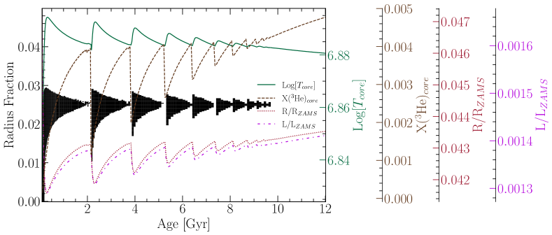
Figure 2: Diagram for a characteristic stellar model of 0.35625 $M_{\odot}$ which is within the Jao Gap’s mass range. The black shaded regions denote whether, at a particular model age, a radial shell within the model is radiative (with white meaning convective). The lines trace the models core temperature, core ³He mass fraction, fractional luminosity wrt. the zero age main sequence and fractional radius wrt. the zero age main sequence.

2.1 Efforts to Model the Gap

Since the identification of the Gap, stellar modeling has been conducted to better constrain its location, effects, and exact cause. Both Mansfield & Kroupa (2021) and Feiden et al. (2021) identify that the Gap’s mass location is correlated with model metallicity — the mass-luminosity discontinuity in lower metallicity models being at a commensurately lower mass. Feiden et al. (2021) suggests this dependence is due to the steep relation of the radiative temperature gradient, $\nabla_{rad}$, on temperature and, in turn, on stellar mass.

$$\nabla_{rad}\propto\frac{L\kappa}{T^{4}}$$ (1)

As metallicity decreases so does opacity, which, by Equation 1, dramatically lowers the temperature at which radiation will dominate energy transport (Chabrier & Baraffe, 1997). Since main sequence stars are virialized the core temperature is proportional to the core density and total mass. Therefore, if the core temperature where convective-kissing instability is expected decreases with metallicity, so too will the mass of stars which experience such instabilities.

The strong opacity dependence of the Jao Gap begs the question: what is the effect of different opacity calculations on Gap properties. As we can see above, changing opacity should affect the Gap’s location in the mass-luminosity relation and therefore in a color-magnitude diagram. Moreover, current models of the Gap have yet to locate it precisely in the CMD (Feiden et al., 2021) with an approximate 0.16 G-magnitude difference between the observed and modeled Gaps. Opacity provides one, as yet unexplored, parameter which has the potential to resolve these discrepancies.

3 Updated Opacities

Multiple groups have released high-temperature opacities including, the Opacity Project (OP Seaton et al., 1994), Laurence Livermore National Labs OPAL opacity tables (Iglesias & Rogers, 1996), and Los Alamos National Labs OPLIB opacity tables (Colgan et al., 2016). OPAL high-temperature radiative opacity tables in particular are very widely used by current generation isochrone grids (e.g. Dartmouth, MIST, & StarEvol, Dotter et al., 2008; Choi et al., 2016; Amard et al., 2019). OPLIB opacity tables (Colgan et al., 2016) are not widely used but include the most up-to-date plasma modeling.

While the overall effect on the CMD of using OPLIB compared to OPAL tables is small, the strong theoretical opacity dependence of the Jao Gap raises the potential for these small effects to measurably shift the Gap’s location. We update DSEP to use high temperature opacity tables based on measurements from Los Alamos national Labs T-1 group (OPLIB, Colgan et al., 2016). The OPLIB tables are created with ATOMIC (Magee et al., 2004; Hakel et al., 2006; Fontes et al., 2015), a modern LTE and non-LTE opacity and plasma modeling code. These updated tables were initially created in order to incorporate the most up to date plasma physics at the time (Bahcall et al., 2005).

OPLIB tables include monochromatic Rosseland mean opacities — composed from bound-bound, bound-free, free-free, and scattering opacities — for elements hydrogen through zinc over temperatures 0.5eV to 100 keV (5802 K – 1.16$\times 10^{9}$ K) and for mass densities from approximately $10^{-8}$ g cm^-3 up to approximately $10^{4}$ g cm^-3 (though the exact mass density range varies as a function of temperature).

DSEP ramps the Ferguson et al. (2005) low temperature opacities to high temperature opacities tables between $10^{4.3}$ K and $10^{4.5}$ K; therefore, only differences between high-temperature opacity sources above $10^{4.3}$ K can effect model evolution. When comparing OPAL and OPLIB opacity tables (Figure 3) we find OPLIB opacities are systematically lower than OPAL opacities for temperatures above $10^{5}$ K. Between $10^{4.3}$ and $10^{5}K$ OPLIB opacities are larger than OPAL opacities. These generally lower opacities will decrease the radiative temperature gradient throughout much of the radius of a model.

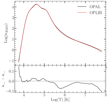
Figure 3: Rosseland mean opacity with the GS98 solar composition for both OPAL opacities and OPLIB opacities (top). Residuals between OPLIB opacities and OPAL opacities (bottom). These opacities are plotted at $\log_{10}(R)=-0.5$, $X=0.7$, and $Z=0.02$. $\log_{10}(R)=-0.5$ approximates much of the interior a 0.35 M_⊙ model. Note how the OPLIB opacities are systematically lower than the OPAL opacities for temperatures above $10^{5.2}$ K.

3.1 Table Querying and Conversion

The high-temperature opacity tables used by DSEP and most other stellar evolution programs give Rosseland-mean opacity, $\kappa_{R}$, along three dimensions: temperature, a density proxy $R$ (Equation 2; $T_{6}=T\times 10^{-6}$, $\rho$ is the mass density), and composition.

$$R=\frac{\rho}{T_{6}^{3}}$$ (2)

OPLIB tables may be queried from a web interface; however, OPLIB opacities are parametrized using mass-density and temperature instead of $R$ and temperature. It is most efficient for us to convert these tables to the OPAL format instead of modifying DSEP to use the OPLIB format directly. In order to generate many tables easily and quickly we develop a web scraper (pyTOPSScrape, Boudreaux, 2022) which can automatically retrieve all the tables needed to build an opacity table in the OPAL format. pyTOPSScrape has been released under the permissive MIT license with the consent of the Los Alamos T-1 group. For a detailed discussion of how the web scraper works and how OPLIB tables are transformed into a format DSEP can use see Appendices A & B.

3.2 Solar Calibrated Stellar Models

In order to validate the OPLIB opacities, we generate a solar calibrated stellar model (SCSM) using these new tables. We first manually calibrate the surface Z/X abundance to within one part in 100 of the solar value (Grevesse & Sauval, 1998, Z/X=0.23). Subsequently, we allow both the convective mixing length parameter, $\alpha_{ML}$, and the initial Hydrogen mass fraction, $X$, to vary simultaneously, minimizing the difference, to within one part in $10^{5}$, between resultant models’ final radius and luminosity to those of the sun. Finally, we confirm that the model’s surface Z/X abundance is still within one part in 100 of the solar value.

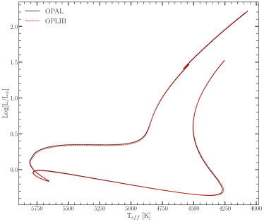
Figure 4: HR Diagram for the two SCSMs, OPAL and OPLIB. OPLIB is shown as a red dashed line.

Solar calibrated stellar models evolved using GS98 OPAL and OPLIB opacity tables (Figure 4) differ $\sim 0.5\%$ in the SCSM hydrogen mass fractions and $\sim 1.5\%$ in the SCSM convective mixing length parameters (Table 1). While the two evolutionary tracks are very similar, note that the OPLIB SCSM’s luminosity is systematically lower past the solar age. While at the solar age the OPLIB SCSM luminosity is effectively the same as the OPAL SCSM. This luminosity difference between OPAL and OPLIB based models is not inconsistent with expectations given the more shallow radiative temperature gradient resulting from the lower OPLIB opacities

Model	$X$	$\alpha_{ML}$
OPAL	0.7066	1.9333
OPLIB	0.7107	1.9629

Table 1: Optimized parameters for SCSMs evolved using OPAL and OPLIB high temperature opacity tables.

4 Modeling

In order to model the Jao Gap we evolve two extremely finely sampled mass grids of models. One of these grids uses the OPAL high-temperature opacity tables while the other uses the OPLIB tables (Figure 5). Each grid evolves a model every 0.00025 $M_{\odot}$ from 0.2 to 0.4 $M_{\odot}$ and every 0.005 $M_{\odot}$ from 0.4 to 0.8 $M_{\odot}$. All models in both grids use a GS98 solar composition, the (1, 101, 0) FreeEOS (version 2.7) configuration, and 1000 year old pre-main sequence polytropic models, with polytropic index 1.5, as their initial conditions. We include gravitational settling in our models where elements are grouped together. Finally, we set a maximum allowed timestep of 50 million years to assure that we fully resolve the build of of core ³He in gap stars.

Despite the alternative view of convection provided by MacDonald & Gizis (2018) discussed in Section 2, given that the mixing timescales in these low mass stars are so short (between $10^{7}$s and $10^{8}$s per Jermyn et al., 2022, Figure 2 & Equation 39, which present the averaged velocity over the convection zone) instantaneous mixing is a valid approximation. Moreover, one principal motivation for a diffusive model of convective mixing has been to account for a deuterium concentration gradient which Chabrier & Baraffe (1997) identify will develop when the deuterium lifetime against proton capture is significantly shorter than the mixing timescale. However, the treatment of energy generation used by DSEP (Bahcall et al., 2001) avoides this issue by computing both the equilibrium deuterium abundance and luminosity of each shell individually, implicitly accounting for the overall luminosity discrepancy identified by Chabrier & Baraffe.

Because in this work we are just interested in the location shift of the Gap as the opacity source varies, we do not model variations in composition. Mansfield & Kroupa (2021); Jao & Feiden (2020); Feiden et al. (2021) all look at the effect composition has on Jao Gap location. They find that as population metallicity increases so too does the mass range and consequently the magnitude of the Gap. From an extremely low metallicity population (Z=0.001) to a population with a more solar like metallicity this shift in mass range can be up to 0.05 M_⊙ (Mansfield & Kroupa, 2021).

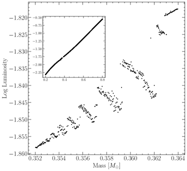
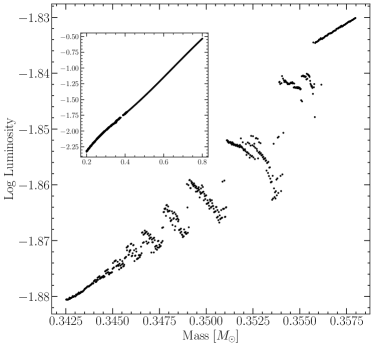
Figure 5: Mass-luminosity relation at 7 Gyrs for models evolved using OPAL opacity tables (top) and those evolved using OPLIB opacity tables (bottom). Note the lower mass range of the OPLIB Gap.

4.1 Population Synthesis

In order to compare the Gap to observations we use in house population synthesis code. We empirically calibrate the relation between G, BP, and RP magnitudes and their uncertainties along with the parallax/G magnitude uncertainty relation using the Gaia Catalouge of Nearby Stas (GCNS, Gaia Collaboration et al., 2021) and Equations 3 & 4. $M_{g}$ is the Gaia G magnitude while $M_{i}$ is the magnitude in the i${}^{\text{th}}$ band, G, BP, or RP. The coefficients $a$, $b$, and $c$ determined using a non-linear least squares fitting routine. Equation 3 then models the relation between G magnitude and parallax uncertainty while Equation 4 models the relation between each magnitude and its uncertainty.

$$\sigma_{plx}(M_{g})=ae^{bM_{g}}+c$$ (3)

$$\sigma_{i}(M_{i})=ae^{M_{i}-b}+c$$ (4)

The full series of steps in our population synthesis code are:

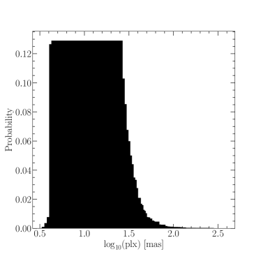
Figure 6: Probability distribution sampled when assigning true parallaxes to synthetic stars. This distribution is built from the GCNS and includes all stars with BP-RP colors between 2.3 and 2.9, the same color range of the Jao Gap.

1. Sample from a Sollima (2019) ($0.25M_{\odot}<M<1M_{\odot}$, $\alpha=-1.34\pm 0.07$) IMF to determine synthetic star mass.

2. Find the closest model above and below the synthetic star, lineally interpolate these models’ $T_{eff}$, $\log(g)$, and $\log(L)$ to those at the synthetic star mass.

3. Convert synthetic star $g$, $T_{eff}$, and $Log(L)$ to Gaia G, BP, and RP magnitudes using the Gaia (E)DR3 bolometric corrections (Creevey et al., 2022) along with code obtained thorough personal communication with Aaron Dotter (Choi et al., 2016).

4. Sample from the GCNS parallax distribution (Figure 6), limited to stars within the BP-RP color range of 2.3 – 2.9, to assign synthetic star a “true” parallax.

5. Use the true parallax to find an apparent magnitude for each filter.

6. Evaluate the empirical calibration given in Equation 3 to find an associated parallax uncertainty. Then sample from a normal distribution with a standard deviation equal to that uncertainty to adjust the true parallax resulting in an “observed” parallax.

7. Use the “observed” parallax and the apparent magnitude to find an “observed” magnitude.

8. Fit the empirical calibration given in Equation 4 to the GCNS and evaluate it to give a magnitude uncertainty scale in each band.

9. Adjust each magnitude by an amount sampled from a normal distribution with a standard deviation of the magnitude uncertainty scale found in the previous step.

This method then incorporates both photometric and astrometric uncertainties into our population synthesis. An example 7 Gyr old synthetic populations using OPAL and OPLIB opacities are presented in Figure 7.

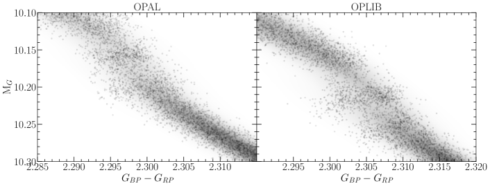
Figure 7: Population synthesis results for models evolved with OPAL (left) and models evolved with OPLIB (right). A Gaussian kernel-density estimate has been overlaid to better highlight the density variations.

4.2 Mixing Length Dependence

In order to test the sensitivity of Gap properties to mixing length we evolve three separate sets OPLIB of models. The first uses a GS98 solar calibrated mixing length, the second uses a mixing length of 1.5, and the third uses a mixing length of 1.0.

We find a clear inverse correlation between mixing length parameter used and the magnitude of the Jao Gap Figures 8 & 9 ($\mu_{G}\propto-1.5\alpha_{ML}$, where $\mu_{G}$ is the mean magnitude of the Gap). This is somewhat surprising given the long established view that the mixing length parameter is of little relevance in fully convective stars (Baraffe et al., 1997). We find an approximate 0.3 magnitude shift in both the color and magnitude comparing a solar calibrated mixing length to a mixing length of 1.5, despite only a 16K difference in effective temperature at 7Gyr between two 0.3 solar mass models. The slight temperature differences between these models are attributable to the steeper adiabatic temperature gradients just below the atmosphere in the solar calibrated mixing length model compared to the $\alpha_{ML}=1.5$ model ($\nabla_{ad,solar}-\nabla_{ad,1.5}\approx 0.05$). Despite this relatively small temperature variance, the large magnitude difference is expected due to the extreme sensitivity of the bolometric corrections on effective temperature at these low temperatures. The mixing length then provides a free parameter which may be used to shift the gap location in order to better match observations without having a major impact on the effective temperature of models. Moreover, recent work indicates that using a solar calibrated mixing length is not appropriate for all stars (e.g. Trampedach et al., 2014; Joyce & Chaboyer, 2018).

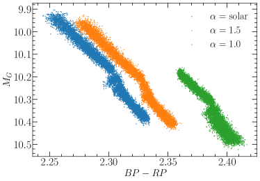
Figure 8: CMD showing OPLIB populations (from left to right) A, B, and C.

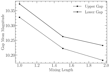
Figure 9: Location of the two identified paucities of stars in OPLIB synthetic populations as a function of the mixing length used.

Given the variability of gap location with mixing length, it is possible that a better fit to the gap location may be achieved through adjustment of the convective mixing length parameter. However, calibrations of the mixing length for stars other than the sun have focused on stars with effective temperature at or above that of the sun and there are no current calibrations of the mixing length parameter for M dwarfs. Moreover, there are additional uncertainties when comparing the predicted gap location to the measured gap location, such as those in the conversion from effective temperature, surface gravity, and luminosity to color, which must be considered if the mixing length is to be used as a gap location free parameter. Given the dangers of freely adjustable parameters and the lack of an a priori expectation for what the convective mixing parameter should be for the population of M Dwarfs in the Gaia DR2 and EDR3 CMD any attempt to use the Jao Gap magnitude to calibrate a mixing length value must be done with caution, and take into account the other uncertainties in the stellar models which could affect the Jao Gap magnitude.

5 Results

We quantify the Jao Gap location along the magnitude (Table 2) axis by sub-sampling our synthetic populations, finding the linear number density along the magnitude axis of each sub-sample, averaging these linear number densities, and extracting any peaks above a prominence threshold of 0.1 as potential magnitudes of the Jao Gap (Figure 10). Gap widths are measured at 50% the height of the peak prominence. We use the python package scipy (Virtanen et al., 2020) to both identify peaks and measure their widths.

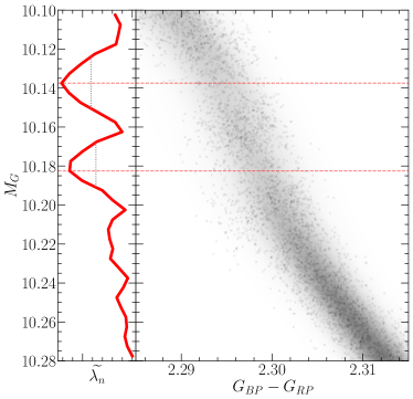
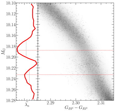
Figure 10: (right panels) OPAL (left) and OPLIB (right) synthetic populations. (left panels) Normalized linear number density along the magnitude axis. A dashed line has been extended from the peak through both panels to make clear where the identified Jao Gap location is wrt. to the population.

Model	Location	Prominence	Width
OPAL 1	10.138	0.593	0.027
OPAL 2	10.183	0.529	0.023
OPLIB 1	10.188	0.724	0.032
OPLIB 2	10.233	0.386	0.027

Table 2: Locations identified as potential Gaps.

In both OPAL and OPLIB synthetic populations our Gap identification method finds two gaps above the prominence threshold. The identification of more than one gap is not inconsistent with the mass-luminosity relation seen in the grids we evolve. As noise is injected into a synthetic population smaller features will be smeared out while larger ones will tend to persist. The mass-luminosity relations shown in in Figure 5 make it clear that there are: (1), multiple gaps due to stars of different masses undergoing convective mixing events at different ages, and (2), the gaps decrease in width moving to lower masses / redder. Therefore, the multiple gaps we identify are attributable to the two bluest gaps being wide enough to not smear out with noise. In fact, if we lower the prominence threshold just slightly from 0.1 to 0.09 we detect a third gap in both the OPAL and OPLIB datasets where one would be expected.

Previous modeling efforts (e.g. Feiden et al., 2021) have not identified multiple gaps. This is likely due to two reasons: (1), previous studies have allowed metallicity to vary across their model grids, further smearing the gaps out, and (2), previous studies have used more coarse underlying mass grids, obscuring features smaller than their mass step. While this dual-gap structure has not been seen in models before, a more complex gap structure is not totally unprecedented as Jao & Feiden (2021) identifies an additional under-dense region below the primary gap in EDR3 data. As part of a follow up series of papers, we are conducting further work to incorporate metallicity variations while still using the finer mass sampling presented here.

The mean gap location of the OPLIB population is at a fainter magnitude than the mean gap location of the OPAL population. Consequently, in the OPLIB sample the convective mixing events which drive the kissing instability begin happening at lower masses (i.e. the convective transition mass decreases). A lower mass range will naturally result in a fainter mean gap magnitude.

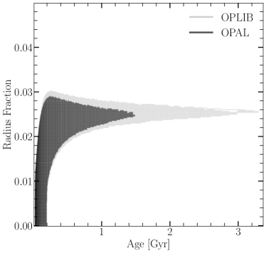
Figure 11: Portions of 0.3526 $M_{\odot}$ OPAL and OPLIB stellar models showing the interior shells which are radiative (black region). Note that for clarity only one convective mixing event from each model is shown. Note how the radiative zone in the OPLIB model is larger.

Mixing events at lower masses in OPLIB models are attributable to the radially thicker, at the same mass, radiative zones (Figure 11). This thicker radiative zone will take more time to break down and is characteristic of OPLIB models as of a result of their slightly lower opacities. A lower opacity fluid will have a more shallow radiative temperature gradient than a higher opacity fluid; however, as the adiabatic temperature gradient remains essentially unchanged as a function of radius, a larger interior radius of the model will remain unstable to radiation. This thicker radiative zone will increase the time it takes the core convective zone to meet up with convective envelope meaning that lower mass models can sustain a radiative zone for longer than they could otherwise; thus; lower opacities push the convective transition mass down. We can additionally see this longer lived radiative zone in the core ³He mass fraction, in which OPLIB models reach much higher concentrations — at approximately the same growth rate — for the same mass as OPAL models do (Figure 12).

The most precise published Gap location comes from Jao & Feiden (2020) who use EDR3 to locate the Gap at $M_{G}\sim 10.3$, we identify the Gap at a similar location in the GCNS data. The Gap in populations evolved using OPLIB tables is closer to this measurement than it is in populations evolved using OPAL tables (Table 2). It should be noted that the exact location of the observed Gap is poorly captured by a single value as the Gap visibly compresses across the width of the main-sequence, wider on the blue edge and narrower on the red edge such that the observed Gap has downward facing a wedge shape (Figure 1). This wedge shape is not successfully reproduced by either any current models or the modeling we preform here. We elect then to specify the Gap location where this wedge is at its narrowest, on the red edge of the main sequence.

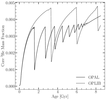
Figure 12: Core ³He mass fraction for 0.3526 $M_{\odot}$ models evolved with OPAL and OPLIB (within the Jao Gap’s mass range for both). Note how the OPLIB model’s core ³He mass fraction grows at approximately the same rate as the OPAL model’s but continues uninterrupted for longer.

The Gaps identified in our modeling have widths of approximately 0.03 magnitudes, while the shift from OPAL to OPLIB opacities is 0.05 magnitudes. With the prior that the Gaps clearly shift before noise is injected we know that this shift is real. However, the shift magnitude and Gap width are of approximately the same size in our synthetic populations. Moreover, Feiden et al. (2021) identify that the shift in the modeled Gap mass from [Fe/H] = 0 to [Fe/H] = +0.5 as 0.04$M_{\odot}$, whereas we only see an approximate $0.01$ M_⊙ shift between OPAL and OPLIB models. Therefore, the Gap location will likely not provide a usable constraint on the opacity source.

6 Conclusion

The Jao Gap provides an intriguing probe into the interior physics of M Dwarfs stars where traditional methods of studying interiors break down. However, before detailed physics may be inferred it is essential to have models which are well matched to observations. Here we investigate whether the OPLIB opacity tables reproduce the Jao Gap location and structure more accurately than the widely used OPAL opacity tables. We find that while the OPLIB tables do shift the Jao Gap location more in line with observations, by approximately 0.05 magnitudes, the shift is small enough that it is likely not distinguishable from noise due to population age and chemical variation. However, future measurement of [Fe/H] for stars within the gap will be helpful in constraining the degree to which the gap should be smeared by these theoretical models.

We also find that both the color and magnitude of the Jao Gap are correlated to the convective mixing length parameter. Specifically, a lower mixing length parameter will bring the gap in the populations presented in this paper more in line with the current best estimate for the actual gap magnitude. Using this relation it may be possible for mixing length to be calibrated for low mass stars such that models match the Jao Gap location. Further, the Jao gap location may provide a test of alternative convection models such as entropy calibrated convection (Spada et al., 2021). Both of these potential uses require careful handeling of other uncertanties such as the uncertanties in bolometric correction, popupulation composition, and population age. As we currently do not have reason to suspect that the mixing length for the low mass stars in the DR2 and ERD3 CMD is substantially lower than that of the sun we leave the investigation of these potential additionl uses for future work.

Finally, we do not find that the OPLIB opacity tables help in reproducing the as yet unexplained wedge shape of the observed Gap.

Appendix A pyTOPSScrape

pyTOPSScrape provides an easy to use command line and python interface for the OPLIB opacity tables accessed through the TOPS web form. Extensive documentation of both the command line and programmatic interfaces is linked in the version controlled repository. However, here we provide a brief, illustrative, example of potential use.

Assuming pyTOPSScrape has been installed and given some working directory which contains a file describing a base composition (“comp.dat”) and another file containing a list of rescalings of that base composition (“rescalings.dat”) (both of these file formats are described in detail in the documentation), one can query OPLIB opacity tables and convert them to a form mimicking that of type 1 OPAL high temperature opacity tables using the following shell command.

Ψ$ generateTOPStables comp.dat rescalings.dat -d ./TOPSCache -o out.opac -j 20

For further examples of pyTOPSScrape please visit the repository.

Appendix B Interpolating $\rho\rightarrow$ R

OPLIB parameterizes $\kappa_{R}$ as a function of mass density, temperature in keV, and composition. Type 1 OPAL high temperature opacity tables, which DSEP and many other stellar evolution programs use, instead parameterizes opacity as a function of temperature in Kelvin, $R$ (Equation B1), and composition. The conversion from temperature in keV to Kelvin is trivial (Equation B2).

$$R=\frac{\rho}{T_{6}^{3}}$$ (B1)

$$T_{K}=T_{keV}*11604525.0061657$$ (B2)

However, the conversion from mass density to $R$ is more involved. Because $R$ is coupled with both mass density and temperature there there is no way to directly convert tabulated values of opacity reported in the OPLIB tables to their equivalents in $R$ space. The TOPS webform does allow for a density range to be specified at a specific temperature, which allows for R values to be directly specified. However, issuing a query to the TOPS webform for not just every composition in a Type 1 OPAL high temperature opacity table but also every temperature for every composition will increase the number of calls to the webform by a factor of 70. Therefore, instead of directly specifying R through the density range we choose to query tables over a broad temperature and density range and then rotate these tables, interpolating $\kappa_{R}(\rho,T_{eff})\rightarrow\kappa_{R}(R,T_{eff})$.

To preform this rotation we use the interp2d function within scipy’s interpolate (Virtanen et al., 2020) module to construct a cubic bivariate B-spline (Dierckx, 1981) interpolating function $s$, with a smoothing factor of 0, representing the surface $\kappa_{R}(\rho,T_{eff})$. For each $R^{i}$ and $T^{j}_{eff}$ reported in type 1 OPAL tables, we evaluate Equation B1 to find $\rho^{ij}=\rho(T^{j}_{eff},R^{i})$. Opacities in $T_{eff}$, $R$ space are then inferred as $\kappa^{ij}_{R}(R^{i},T^{j}_{eff})=s(\rho^{ij},T^{j}_{eff})$.

As first-order validation of this interpolation scheme we can preform a similar interpolation in the opposite direction, rotating the tables back to $\kappa_{R}(\rho,T_{eff})$ and then comparing the initial, “raw”, opacities to those which have gone through the interpolations process. Figure 13 shows the fractional difference between the raw opacities and a set which have gone through this double interpolation. The red line denotes $\log(R)=-0.79$ where models near the Jao Gap mass range will tend to sit for much of their radius. Along the $\log(R)=-0.79$ line the mean fractional difference is $\langle\delta\rangle=0.005$ with an uncertainty of $\sigma_{\langle\delta\rangle}=0.013$. One point of note is that, because the initial rotation into $\log(R)$ space also reduces the domain of the opacity function, interpolation-edge effects which we avoid initially by extending the domain past what type 1 OPAL tables include cannot be avoided when interpolating back into $\rho$ space.

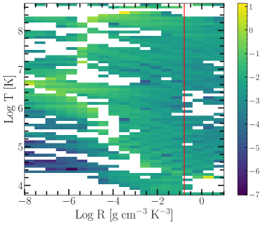
Figure 13: Log Fractional Difference between opacities in $\kappa_{R}(\rho,T_{eff})$ space directly queried from the OPLIB web-form and those which have been interpolated into $\log(R)$ space and back. Note that, due to the temperature grid of type 1 OPAL tables not aligning perfectly which the temperature grid OPLIB uses there may be edge effects where the interpolation is poorly constrained. The red line corresponds to $\log(R)=-0.79$ where much of a stellar model’s radius exists.

References

- Amard et al. (2019) Amard, L., Palacios, A., Charbonnel, C., et al. 2019, A&A, 631, A77, doi: 10.1051/0004-6361/201935160
- Bahcall et al. (2001) Bahcall, J. N., Pinsonneault, M. H., & Basu, S. 2001, ApJ, 555, 990, doi: 10.1086/321493
- Bahcall et al. (2005) Bahcall, J. N., Serenelli, A. M., & Basu, S. 2005, ApJ, 621, L85, doi: 10.1086/428929
- Baraffe & Chabrier (2018) Baraffe, I., & Chabrier, G. 2018, A&A, 619, A177, doi: 10.1051/0004-6361/201834062
- Baraffe et al. (1997) Baraffe, I., Chabrier, G., Allard, F., & Hauschildt, P. H. 1997, A&A, 327, 1054. https://arxiv.org/abs/astro-ph/9704144
- Boudreaux (2022) Boudreaux, T. 2022, tboudreaux/pytopsscrape: pyTOPSScrape v1.0, v1.0, Zenodo, doi: 10.5281/zenodo.7094198
- Chabrier & Baraffe (1997) Chabrier, G., & Baraffe, I. 1997, A&A, 327, 1039. https://arxiv.org/abs/astro-ph/9704118
- Chandra & Varanasi (2015) Chandra, R. V., & Varanasi, B. S. 2015, Python requests essentials (Packt Publishing Ltd)
- Choi et al. (2016) Choi, J., Dotter, A., Conroy, C., et al. 2016, ApJ, 823, 102, doi: 10.3847/0004-637X/823/2/102
- Colgan et al. (2016) Colgan, J., Kilcrease, D. P., Magee, N. H., et al. 2016, in APS Meeting Abstracts, Vol. 2016, APS Division of Atomic, Molecular and Optical Physics Meeting Abstracts, D1.008
- Creevey et al. (2022) Creevey, O. L., Sordo, R., Pailler, F., et al. 2022, arXiv e-prints, arXiv:2206.05864. https://arxiv.org/abs/2206.05864
- Dierckx (1981) Dierckx, P. 1981, IMA Journal of Numerical Analysis, 1, 267, doi: 10.1093/imanum/1.3.267
- Dotter et al. (2008) Dotter, A., Chaboyer, B., Jevremović, D., et al. 2008, The Astrophysical Journal Supplement Series, 178, 89
- Feiden et al. (2021) Feiden, G. A., Skidmore, K., & Jao, W.-C. 2021, ApJ, 907, 53, doi: 10.3847/1538-4357/abcc03
- Ferguson et al. (2005) Ferguson, J. W., Alexander, D. R., Allard, F., et al. 2005, ApJ, 623, 585, doi: 10.1086/428642
- Fontes et al. (2015) Fontes, C. J., Zhang, H. L., Abdallah, J., J., et al. 2015, Journal of Physics B Atomic Molecular Physics, 48, 144014, doi: 10.1088/0953-4075/48/14/144014
- Gaia Collaboration et al. (2021) Gaia Collaboration, Smart, R. L., Sarro, L. M., et al. 2021, A&A, 649, A6, doi: 10.1051/0004-6361/202039498
- Grevesse & Sauval (1998) Grevesse, N., & Sauval, A. J. 1998, Space Sci. Rev., 85, 161, doi: 10.1023/A:1005161325181
- Hakel et al. (2006) Hakel, P., Sherrill, M. E., Mazevet, S., et al. 2006, J. Quant. Spec. Radiat. Transf., 99, 265, doi: 10.1016/j.jqsrt.2005.04.007
- Iglesias & Rogers (1996) Iglesias, C. A., & Rogers, F. J. 1996, ApJ, 464, 943, doi: 10.1086/177381
- Irwin (2012) Irwin, A. W. 2012, FreeEOS: Equation of State for stellar interiors calculations, Astrophysics Source Code Library, record ascl:1211.002. http://ascl.net/1211.002
- Jao & Feiden (2020) Jao, W.-C., & Feiden, G. A. 2020, AJ, 160, 102, doi: 10.3847/1538-3881/aba192
- Jao & Feiden (2021) —. 2021, Research Notes of the American Astronomical Society, 5, 124, doi: 10.3847/2515-5172/ac053a
- Jao et al. (2018) Jao, W.-C., Henry, T. J., Gies, D. R., & Hambly, N. C. 2018, ApJ, 861, L11, doi: 10.3847/2041-8213/aacdf6
- Jermyn et al. (2022) Jermyn, A. S., Bauer, E. B., Schwab, J., et al. 2022, arXiv e-prints, arXiv:2208.03651. https://arxiv.org/abs/2208.03651
- Joyce & Chaboyer (2018) Joyce, M., & Chaboyer, B. 2018, ApJ, 864, 99, doi: 10.3847/1538-4357/aad464
- MacDonald & Gizis (2018) MacDonald, J., & Gizis, J. 2018, MNRAS, 480, 1711, doi: 10.1093/mnras/sty1888
- Magee et al. (2004) Magee, N. H., Abdallah, J., Colgan, J., et al. 2004, in American Institute of Physics Conference Series, Vol. 730, Atomic Processes in Plasmas: 14th APS Topical Conference on Atomic Processes in Plasmas, ed. J. S. Cohen, D. P. Kilcrease, & S. Mazavet, 168–179, doi: 10.1063/1.1824868
- Mansfield & Kroupa (2021) Mansfield, S., & Kroupa, P. 2021, A&A, 650, A184, doi: 10.1051/0004-6361/202140536
- Nutzman & Charbonneau (2008) Nutzman, P., & Charbonneau, D. 2008, PASP, 120, 317, doi: 10.1086/533420
- Richardson (2007) Richardson, L. 2007, April
- Rodríguez-López (2019) Rodríguez-López, C. 2019, Frontiers in Astronomy and Space Sciences, 6, 76, doi: 10.3389/fspas.2019.00076
- Seaton et al. (1994) Seaton, M. J., Yan, Y., Mihalas, D., & Pradhan, A. K. 1994, MNRAS, 266, 805, doi: 10.1093/mnras/266.4.805
- Skrutskie et al. (2006) Skrutskie, M. F., Cutri, R. M., Stiening, R., et al. 2006, AJ, 131, 1163, doi: 10.1086/498708
- Sollima (2019) Sollima, A. 2019, Monthly Notices of the Royal Astronomical Society, 489, 2377, doi: 10.1093/mnras/stz2093
- Spada et al. (2021) Spada, F., Demarque, P., & Kupka, F. 2021, MNRAS, 504, 3128, doi: 10.1093/mnras/stab1106
- Trampedach et al. (2014) Trampedach, R., Stein, R. F., Christensen-Dalsgaard, J., Nordlund, Å., & Asplund, M. 2014, MNRAS, 445, 4366, doi: 10.1093/mnras/stu2084
- van Saders & Pinsonneault (2012) van Saders, J. L., & Pinsonneault, M. H. 2012, ApJ, 751, 98, doi: 10.1088/0004-637X/751/2/98
- Virtanen et al. (2020) Virtanen, P., Gommers, R., Oliphant, T. E., et al. 2020, Nature Methods, 17, 261, doi: 10.1038/s41592-019-0686-2