Flavor Physics Constraints on Left-Right Symmetric Models with Universal Seesaw

Abstract

We study the phenomenological constraints on the parameter space in the parity symmetric scenario of a class of left-right symmetric models in which the fermion masses are generated through a universal seesaw mechanism. The model, motivated by the axionless solution to the strong $\mathcal{CP}$ problem, has a simple Higgs sector consisting of left- and right-handed doublets. The fermion masses are then generated through their mixing with heavy vector-like fermions, which leads to flavor changing neutral currents arising at tree-level and also introduces non-unitarity in the charged current interactions. These new contributions lead to flavor and flavor universality violating processes and forbidden decays, which are used to derive constraints on the parameter space of the model. We also argue that although the model has the potential to resolve flavor anomalies, it fails to do so in the case of B-anomalies $R_{K^{(*)}}$ and anomalous magnetic moment of muon $(g-2)_{\mu}$.

1 Introduction

The left-right symmetric models (LRSMs) are simple extensions of the standard model (SM), initially proposed as a solution to the parity asymmetry observed at low energy scales, involving the symmetry group $SU(3)_{c}\times SU(2)_{L}\times SU(2)_{R}\times U(1)_{B-L}$. The LRSMs, based on the concept that the $V-A$ structure of weak interaction may be a low-energy phenomenon that vanishes at very high energy scales of the order of a few TeV, overcome this by putting both left- and right-handed particles on equal footing thereby restoring the symmetry Pati:1974yy ; Mohapatra:1974gc ; Senjanovic:1975rk . Such models have several attractive features. Right-handed neutrinos arise naturally, generating light neutrino masses through seesaw mechanism Minkowski:1977sc ; GellMann:1980vs ; Mohapatra:1979ia ; Yanagida:1980xy ; Schechter:1980gr ; Glashow:1979nm ; Mohapatra:2004zh . These models also give a physical interpretation of the hypercharge as a quantity arising from the $B-L$ quantum number.

The class of LRSMs discussed in this paper is motivated by the axionless solution to the strong $\mathcal{CP}$ problem Babu:1989rb since parity is a good symmetry broken spontaneously Beg:1978mt . The fermion masses in these models are induced through a universal seesaw mechanism Berezhiani:1983hm ; Davidson:1987mh ; Babu:1988mw by introducing heavy vector-like fermionic (VLF) singlet partners. The scalar sector of the model is minimal, containing only two Higgs doublets. The light fermion masses are quadratically dependent on Yukawa couplings ($\mathcal{Y}_{i}$), allowing for the values of $\mathcal{Y}_{i}$ required to explain fermion mass hierarchy to be in the range $\mathcal{Y}_{i}=(10^{-3}-1)$ as opposed to $\mathcal{Y}_{i}=(10^{-6}-1)$ in SM or standard LRSMs. Another exciting feature of the LRSMs is the flavor-changing neutral current (FCNC) interactions leading to flavor-violating processes occurring at the tree level due to direct couplings between VLFs and SM fermions. There can also be corrections to the SM charged current interactions. These can result in stringent constraints on the parameter space of the model which are explored in great detail in this work. The model can also potentially resolve the recent flavor anomalies such as $(g-2)_{\mu}$, $R_{K^{(*)}}$, $R_{D^{(*)}}$, CDF-$W$ mass shift and the Cabibbo anomaly. This model has also been studied recently in the context of low energy experimental signals Craig:2020bnv , gravitational waves Graf:2021xku , neutrino oscillations Babu:2020bgz and, in explaining CKM unitarity problem and CDF $W$-boson mass Babu:2022jbn .

Several measurements of semi-leptonic decays of B mesons have shown significant deviations from their SM predicted values Bobeth:2007dw ; Bordone:2016gaq . The most notable ones are the lepton flavor universality (LFU) violation observed in the neutral current transitions related to the ratio $R_{K^{(*)}}=\text{BR}(B\to K^{(*)}\mu\mu)/\text{BR}(B\to K^{(*)}ee)$ and in charged current mediated $R_{D^{(*)}}=\text{BR}(B\to D^{(*)}\tau\nu_{\tau})/\text{BR}(B\to D^{(*)}\ell\nu_{\ell})$, $\ell=e,\leavevmode\nobreak\ \mu$. These are theoretically clean observables since the hadronic uncertainties cancel out in the ratios, making them extremely sensitive to new physics probes. Deviations in the measurements of $R_{D^{(*)}}$ and $R_{K^{(*)}}$ Aaij:2017vbb ; Abdesselam:2019wac ; Aaij:2019wad ; LHCb:2021trn from the SM are collectively referred to as B-anomalies. A solution to $R_{D^{(*)}}$ anomaly using this model has been discussed in Babu:2018vrl . The most precise measurement of $R_{K}$ has resulted in a combined $3.1\leavevmode\nobreak\ \sigma$ discrepancy in $R_{K^{(*)}}$ and related processes. As a natural consequence of parity invariance, a right-handed neutral gauge boson exists that mixes with the SM $Z$ boson giving rise to two neutral gauge boson eigenstates, $Z_{1}$ and $Z_{2}$. Both these gauge bosons can mediate tree-level FCNC processes that contribute to $R_{K^{(*)}}$ to occur at the tree level. Hence, the LRSM model can potentially resolve the neutral current B-anomalies as well.

Another major hint towards physics beyond the SM comes from the long-standing discrepancy between the experiment and theory in the anomalous magnetic moment (AMM) of muon, $a_{\mu}$. The most recent measurement of $a_{\mu}$ at Fermilab National Accelerator Laboratory (FNAL) reports a $4.2\,\sigma$ deviation from the SM predicted value of AMM. The model explored in this work can provide chirally enhanced one-loop corrections to AMM of muon mediated by neutral scalar ($h,\,H$) or gauge ($Z_{1},\,Z_{2}$) fields. The possibility of resolving the anomaly in muon AMM is explored briefly in this paper.

In this work, we look at the flavor physics constraints on the model, exploring the allowed parameter space from neutral current gauge interactions, investigate the most stringent constraints for charged current and Higgs interactions, and address the limitations of the model in resolving $R_{K^{(*)}}$ discrepancies as well as the AMM of muon. The rest of the paper is organized as follows. We describe the details of the LRSM model Babu:2018vrl , giving the particle content, Higgs potential and gauge boson mass matrix diagonalization in Sec. 2 and the fermion mass matrix diagonalizations and their interaction Lagrangian in the physical basis in Sec. 3. In Secs. 4, 5, and 6, we list the different constraints on the model parameters obtained from neutral and charged current gauge interactions, and scalar interactions, respectively, in the parity symmetric scenario of the model. In Sec. 7, we explore the solution to neutral current B-anomalies arising at tree-level mediated by the neutral gauge bosons, and at one-loop level mediated by the left-handed scalar doublet. Sec. 8 examines the VL-lepton mass-enhanced corrections to the AMM of muon at one-loop level mediated by the neutral gauge as well as scalar fields, and we conclude with Sec. 9.

2 Model Description

The particle spectrum of the LRSM with universal seesaw is composed of the usual SM fermions, right-handed neutrinos, and four sets of vector-like singlet fermions, denoted as $(U_{a},D_{a},E_{a},N_{a})$, where, the index $a$ runs from 1 to 3 for the three generations of fermions. The SM fermions, along with the right-handed neutrinos, form left- or right-handed doublets, assigned to the gauge group $SU(3)_{c}\times SU(2)_{L}\times SU(2)_{R}\times U(1)_{B-L}$ as follows ($i=1-3$ is the family index):

$$\mathcal{Q}_{L,i}\left(3,2,1,+\frac{1}{3}\right)=\begin{pmatrix}u_{L}\\ d_{L}\end{pmatrix}_{i}, \mathcal{Q}_{R,i}\left(3,1,2,+\frac{1}{3}\right)=\begin{pmatrix}u_{R}\\ d_{R}\end{pmatrix}_{i},$$ (2.1)

$$\psi_{L,i}\left(1,2,1,-1\right)=\begin{pmatrix}\nu_{L}\\ e_{L}\end{pmatrix}_{i}, \psi_{R,i}\left(1,1,2,-1\right)=\begin{pmatrix}\nu_{R}\\ e_{R}\end{pmatrix}_{i}.$$

The Higgs sector is comprised simply of left- and right-handed doublets:

$$\chi_{L}\left(1,2,1,+1\right)=\begin{pmatrix}\chi_{L}^{+}\\ \chi_{L}^{0}\end{pmatrix}, \chi_{R}\left(1,1,2,+1\right)=\begin{pmatrix}\chi_{R}^{+}\\ \chi_{R}^{0}\end{pmatrix}.$$ (2.2)

$\sigma_{L}=Re(\chi_{L}^{0})/\sqrt{2}$ and $\sigma_{R}=Re(\chi_{R}^{0})/\sqrt{2}$ are the neutral scalar fields which mix to give the SM-like Higgs boson $h$ (125 GeV) and a heavy $H$. In the limit of small mixing, the SM Higgs is identified as $\sigma_{L}$. The general Higgs potential is given by

$$V=-(\mu_{L}^{2}\chi_{L}^{\dagger}\chi_{L}+\mu_{R}^{2}\chi_{R}^{\dagger}\chi_{R})+\frac{\lambda_{1L}}{2}(\chi_{L}^{\dagger}\chi_{L})^{2}+\frac{\lambda_{1R}}{2}(\chi_{R}^{\dagger}\chi_{R})^{2}+\lambda_{2}(\chi_{L}^{\dagger}\chi_{L})(\chi_{R}^{\dagger}\chi_{R}).$$ (2.3)

In the parity symmetric limit, $\lambda_{1L}=\lambda_{1R}$, but $\mu_{L}$ can be allowed to be different from $\mu_{R}$ since parity can be softly broken. The vacuum expectation values of the neutral fields for which the potential Eq. (2.3) has a minimum are denoted by

$$\left\langle\chi_{L}^{0}\right\rangle=\kappa_{L}, \left\langle\chi_{R}^{0}\right\rangle=\kappa_{R},$$ (2.4)

with $\kappa_{L}\simeq 174$ GeV. The remaining fields are ?eaten up? by $W_{L,R}^{\pm}$ and $Z_{L,R}$ bosons upon symmetry breaking. The physical Higgs spectrum obtained from the diagonalization of $\sigma_{L}-\sigma_{R}$ mixing matrix,

$$\mathcal{M}^{2}_{\sigma_{L,R}}=\begin{bmatrix}2\lambda_{1L}\kappa_{L}^{2}&&2\lambda_{2}\kappa_{L}\kappa_{R}\\ 2\lambda_{2}\kappa_{L}\kappa_{R}&&2\lambda_{1R}\kappa_{R}^{2},\end{bmatrix},$$ (2.5)

are as follows:

$$h=\cos\zeta\sigma_{L}-\sin\zeta\sigma_{R}, H=\sin\zeta\sigma_{L}+\cos\zeta\sigma_{R},$$ (2.6)

$$M_{h}^{2}\simeq 2\lambda_{1L}\left(1-\frac{\lambda_{2}^{2}}{\lambda_{1L}\lambda_{1R}}\right)\kappa_{L}^{2}, M_{H}^{2}=2\lambda_{1R}\kappa_{R}^{2},$$

with the mixing angle $\zeta$ given by

$$\tan 2\zeta=\frac{2\lambda_{2}\kappa_{L}\kappa_{R}}{(\lambda_{1R}\kappa_{R}^{2}-\lambda_{1L}\kappa_{L}^{2})}.$$ (2.7)

To generate the fermion masses in the absence of the Higgs bidoublet $(1,2,2,0)$ seen in the standard LRSMs, vector-like fermions (VLFs) are introduced. The gauge quantum numbers of the VLFs are

$$U_{a}\left(3,1,1,+\frac{4}{3}\right), D_{a}\left(3,1,1,-\frac{2}{3}\right), E_{a}\left(1,1,1,-2\right), N_{a}\left(1,1,1,0\right),$$ (2.8)

The electric charge is given by

$$Q= T_{3L}+T_{3R}+\frac{B-L}{2}\text{ with,}$$ (2.9)

$$\frac{Y}{2}= T_{3R}+\frac{B-L}{2},$$

thereby giving the hypercharge a definition in terms of the $SU(2)_{R}$ and $U(1)_{B-L}$ quantum numbers. Defining the covariant derivative as

$$D_{\mu}=\partial_{\mu}+i\frac{g_{L,R}}{2}(\vec{\tau}.\overrightarrow{W}_{L,R\mu})+ig_{B}\frac{B-L}{2}B_{\mu},$$ (2.10)

the interaction of gauge bosons with Higgs field can be derived from the kinetic term of the Lagrangian

$$\mathcal{L}^{\text{KE}}_{\text{Higgs}}=(D_{\mu}\chi_{L})^{\dagger}(D_{\mu}\chi_{L})+(D_{\mu}\chi_{R})^{\dagger}(D_{\mu}\chi_{R}).$$ (2.11)

It can be easily verified that the charged gauge bosons do not mix at tree level, and their masses are

$$M^{2}_{W^{\pm}_{L(R)}}=\frac{1}{2}g_{L(R)}^{2}\kappa_{L(R)}^{2}.$$ (2.12)

Of the neutral gauge bosons, the photon field $A_{\mu}$ remains massless while the two orthogonal fields $Z_{L}$ and $Z_{R}$ mix. In the limit of small $\kappa_{L}$, these fields are related to the gauge eigenstates by:

$$A^{\mu} =\frac{g_{L}g_{R}B^{\mu}+g_{B}g_{R}W^{\mu}_{3L}+g_{B}g_{L}W^{\mu}_{3R}}{\sqrt{g_{B}^{2}(g_{L}^{2}+g_{R}^{2})+g_{L}^{2}g_{R}^{2}}},$$ (2.13)

$$Z^{\mu}_{R} =\frac{g_{B}B^{\mu}-g_{R}W^{\mu}_{3R}}{\sqrt{g_{R}^{2}+g_{B}^{2}}},$$

$$Z^{\mu}_{L} =\frac{g_{B}g_{R}B^{\mu}-g_{L}g_{R}\left(1+\frac{g_{B}^{2}}{g_{R}^{2}}\right)W^{\mu}_{3L}+g_{B}^{2}W^{\mu}_{3R}}{\sqrt{g_{B}^{2}+g_{R}^{2}}\sqrt{g_{B}^{2}+g_{L}^{2}+\frac{g_{B}^{2}g_{L}^{2}}{g_{R}^{2}}}}.$$

The hypercharge relation implies $g_{Y}^{-2}=g_{R}^{-2}+g_{B}^{-2}$, which can be used to eliminate $g_{B}$ in terms of $g_{Y}$ resulting in the $Z_{L}-Z_{R}$ mixing matrix

$$\mathcal{M}^{2}_{Z_{L}-Z_{R}}=\frac{1}{2}\begin{pmatrix}(g_{L}^{2}+g_{Y}^{2})\kappa_{L}^{2}&&g_{Y}^{2}\sqrt{\frac{g_{L}^{2}+g_{Y}^{2}}{g_{R}^{2}-g_{Y}^{2}}}\kappa_{L}^{2}\\ g_{Y}^{2}\sqrt{\frac{g_{L}^{2}+g_{Y}^{2}}{g_{R}^{2}-g_{Y}^{2}}}\kappa_{L}^{2}&&\frac{g_{R}^{4}\kappa_{R}^{2}+g_{Y}^{4}\kappa_{L}^{2}}{g_{R}^{2}-g_{Y}^{2}}\end{pmatrix},$$ (2.14)

from which the physical states and masses can be obtained as:

$$Z_{1}=\cos\xi Z_{L}-\sin\xi Z_{R}, \quad\quad Z_{2}=\sin\xi Z_{L}+\cos\xi Z_{R},$$ (2.15)

$$M^{2}_{Z_{1}}\simeq\frac{1}{2}(g_{Y}^{2}+g_{L}^{2})\kappa_{L}^{2}, \quad\quad M^{2}_{Z_{2}}\simeq\frac{g_{R}^{4}}{2(g_{R}^{2}-g_{Y}^{2})}\kappa_{R}^{2}+\frac{g_{Y}^{4}}{2(g_{R}^{2}-g_{Y}^{2})}\kappa_{L}^{2},$$

and the mixing angle is given by $\xi\simeq\frac{g_{Y}^{2}}{g_{R}^{4}}\frac{\kappa_{L}^{2}}{\kappa_{R}^{2}}\sqrt{(g_{L}^{2}+g_{Y}^{2})(g_{R}^{2}-g_{Y}^{2})}$ or more accurately,

$$\tan(-2\xi)=\frac{2g_{Y}^{2}\sqrt{(g_{L}^{2}+g_{Y}^{2})(g_{R}^{2}-g_{Y}^{2})}\kappa_{L}^{2}}{g_{R}^{4}\kappa_{R}^{2}+g_{Y}^{4}\kappa_{L}^{2}-(g_{L}^{2}+g_{R}^{2})(g_{R}^{2}-g_{Y}^{2})\kappa_{L}^{2}}.$$ (2.16)

The SM $Z$ boson of mass $91.18$ GeV is identified to be $Z_{1}$ or, in the limit of small mixing angle, $Z_{L}$. $Z_{1}$ and $Z$ will be used interchangeably, henceforth.

3 Interactions among Physical Fields

In this section, the diagonalization of fermion mass matrices is studied and the fermionic interactions with the bosonic fields are explored.

3.1 Charged Fermions

The Yukawa interactions of the charged fermions in the flavor basis is given by

$$\mathcal{L}_{\text{Yuk}} =\mathcal{Y}_{U}\overline{\mathcal{Q}}_{L}\widetilde{\chi}_{L}U_{R}+\mathcal{Y}^{\prime}_{U}\overline{\mathcal{Q}}_{R}\widetilde{\chi}_{R}U_{L}+M_{U}\overline{U}_{L}U_{R}$$ (3.17)

$$+\mathcal{Y}_{D}\overline{\mathcal{Q}}_{L}\chi_{L}D_{R}+\mathcal{Y}^{\prime}_{D}\overline{\mathcal{Q}}_{R}\chi_{R}D_{L}+M_{D}\overline{D}_{L}D_{R}$$

$$+\mathcal{Y}_{E}\overline{\psi}_{L}\chi_{L}E_{R}+\mathcal{Y}^{\prime}_{E}\overline{\psi}_{R}\chi_{R}E_{L}+M_{E}\overline{E}_{L}E_{R}+\mathrm{h.c.}$$

with $\widetilde{\chi}_{L,R}=i\tau_{2}\chi^{*}_{L,R}$. Under parity symmetry, $\mathcal{Y}=\mathcal{Y}^{\prime}$ and $M=M^{\dagger}$. The above Lagrangian gives $6\times 6$ mass matrices for up-type quarks $(u,U)$, down-type quarks $(d,D)$ and charged leptons $(e,E)$ which are written in the form:

$$\mathcal{M}_{U,D,E}=\begin{pmatrix}0&\mathcal{Y}_{U,D,E}\kappa_{L}\\ \mathcal{Y}^{\prime\dagger}_{U,D,E}\kappa_{R}&M_{U,D,E}\end{pmatrix}.$$ (3.18)

Matrices of the form $\mathcal{M}$ can be block-diagonalized by a bi-unitary transform with two unitary matrices parametrized by $\rho_{L}$ and $\rho_{R}$.

$$\mathcal{U}_{X}=\begin{pmatrix}\mathds{1}-\frac{1}{2}\rho^{\dagger}_{X}\rho_{X}&&\rho^{\dagger}_{X}\\ -\rho_{X}&&\mathds{1}-\frac{1}{2}\rho_{X}\rho^{\dagger}_{X}\end{pmatrix},\,\,X=\{L,R\}.$$ (3.19)

$\rho_{L}$ is necessarily small while we assume $\rho_{R}\ll 1$ as well, to simplify the analysis.

$$\mathcal{M}_{\text{diag}}=\begin{pmatrix}\mathds{1}-\frac{1}{2}\rho^{\dagger}_{L}\rho_{L}&&-\rho^{\dagger}_{L}\\ \rho_{L}&&\mathds{1}-\frac{1}{2}\rho_{L}\rho^{\dagger}_{L}\end{pmatrix}\begin{pmatrix}0&\mathcal{Y}\kappa_{L}\\ \mathcal{Y}^{\prime\dagger}\kappa_{R}&M\end{pmatrix}\begin{pmatrix}\mathds{1}-\frac{1}{2}\rho^{\dagger}_{R}\rho_{R}&&\rho^{\dagger}_{R}\\ -\rho_{R}&&\mathds{1}-\frac{1}{2}\rho_{R}\rho^{\dagger}_{R}\end{pmatrix},$$ (3.20)

where the matrices $\mathcal{U}_{L,R}$ are unitary up to $\mathcal{O}(\rho^{2})$, and the parameters are related to the masses and Yukawa interactions by

$$\rho_{L}=\kappa_{L}M^{-1\dagger}\mathcal{Y}^{\dagger},$$ (3.21)

$$\rho_{R}=\kappa_{R}M^{-1}\mathcal{Y}^{\prime\dagger},$$

while the mass eigenvalues are

$$\hat{m}=-\kappa_{L}\kappa_{R}\mathcal{Y}M^{-1}\mathcal{Y}^{\prime\dagger}, \hat{M}=M+\frac{1}{2}(\kappa_{R}^{2}\mathcal{Y}^{\prime\dagger}\mathcal{Y}^{\prime}M^{-1\dagger}+\kappa_{L}^{2}M^{-1\dagger}\mathcal{Y}^{\dagger}\mathcal{Y}).$$ and (3.22)

$M$ is assumed to be diagonal while $\hat{m}$ needs to be diagonalized by a subsequent bi-unitary transform such that $m_{f}=V_{L_{f}}\hat{m}V^{\dagger}_{R_{f}}$. Now, it is possible to write the interactions of charged fermions with gauge and scalar bosons in the mass basis. In the following sections, $f(\ell)$ stands for mass eigenstate of charged fermions (leptons), and $F$, $U$, $D$, and $E$ represent charged VLF.

3.1.1 Neutral Current

The tree-level interactions of charged fermions in their mass basis with the neutral gauge bosons are:

$$-g_{Z_{L}}^{-1}\mathcal{L}_{Z_{L}} =\overline{f}_{L}\gamma^{\mu}Z_{L_{\mu}}\left(A_{L}-(A_{L}-B_{L})V_{L_{f}}\rho_{L_{F}}^{\dagger}\rho_{L_{F}}V^{\dagger}_{L_{f}}\right)f_{L}$$ (3.23)

$$+\overline{f}_{R}\gamma^{\mu}Z_{L_{\mu}}\left(A_{L}^{\prime}\right)f_{R}$$

$$+\overline{f}_{L}\gamma^{\mu}Z_{L_{\mu}}\left((A_{L}-B_{L})V_{L_{f}}\rho_{L_{F}}^{\dagger}\right)F_{L}$$

$$+\overline{F}_{L}\gamma^{\mu}Z_{L_{\mu}}\left((A_{L}-B_{L})\rho_{{}_{L}F}V^{\dagger}_{L_{f}}\right)f_{L}$$

$$+\overline{F}_{L,R}\gamma^{\mu}Z_{L_{\mu}}\left(B_{L}\right)F_{L,R},$$

$$-g_{Z_{R}}^{-1}\mathcal{L}_{Z_{R}} =\overline{f}_{L}\gamma^{\mu}Z_{R_{\mu}}\left(A_{R}-(A_{R}-B_{R})V_{L_{f}}\rho_{L_{F}}^{\dagger}\rho_{L_{F}}V^{\dagger}_{L_{f}}\right)f_{L}$$ (3.24)

$$+\overline{f}_{L}\gamma^{\mu}Z_{R_{\mu}}\left((A_{R}-B_{R})V_{L_{f}}\rho_{L_{F}}^{\dagger}\right)F_{L}$$

$$+\overline{F}_{L}\gamma^{\mu}Z_{R_{\mu}}\left((A_{R}-B_{R})\rho_{L_{F}}V^{\dagger}_{L_{f}}\right)f_{L}$$

$$+\{L\to R\text{ with }A_{R}\to A_{R}^{\prime}\}$$

$$+\overline{F}_{L,R}\gamma^{\mu}Z_{R_{\mu}}\left(B_{R}\right)F_{L,R},$$

where,

$$g_{Z_{L,R}}=\frac{g_{L,R}^{2}}{\sqrt{g_{L,R}^{2}\pm g_{Y}^{2}}}\leavevmode\nobreak\ \leavevmode\nobreak\ \leavevmode\nobreak\ , \leavevmode\nobreak\ \leavevmode\nobreak\ \leavevmode\nobreak\ \leavevmode\nobreak\ \leavevmode\nobreak\ B_{L,R}=-\frac{g_{Y}^{2}}{g_{L,R}^{2}}\frac{Y_{F}}{2},$$ (3.25)

$$A_{L,R}=T_{3L,3R}-\frac{g_{Y}^{2}}{g_{L,R}^{2}}\frac{Y_{f_{L,R}}}{2}, \leavevmode\nobreak\ \leavevmode\nobreak\ \leavevmode\nobreak\ \leavevmode\nobreak\ \leavevmode\nobreak\ \leavevmode\nobreak\ \leavevmode\nobreak\ \leavevmode\nobreak\ \leavevmode\nobreak\ \leavevmode\nobreak\ A^{\prime}_{L,R}=-\frac{g_{Y}^{2}}{g_{L,R}^{2}}\frac{Y_{f_{R,L}}}{2}.$$

$Y_{f_{L,R}}$ are the hypercharges of SM fermions and $Y_{F}$ is the hypercharge of the VLF. Under parity symmetry, $g_{R}=g_{L}$, $V_{R_{f}}=V_{L_{f}}$ and $\rho_{R}=\frac{\kappa_{R}}{\kappa_{L}}\rho_{L}$. The SM interaction of charged fermions to $Z$ boson can be obtained from $\mathcal{L}_{Z_{L}}$ as the VLF decouples from SM fermions. The above expressions can be converted into the mass basis of the neutral gauge bosons using the relations in Eq. (2.15), as shown in Eqs. (4.44) and (4.45) with the couplings given in Appendix. A.

3.1.2 Charged Current

The charged current interactions of quarks are given by

$$-\frac{\sqrt{2}}{g_{L}}\mathcal{L}_{W_{X}} =\overline{u}_{X}\gamma^{\mu}W^{+}_{X\mu}\Bigl{(}V_{X_{u}}V_{X_{d}}^{\dagger}-\frac{1}{2}(V_{X_{u}}\rho_{X_{D}}^{\dagger}\rho_{X_{D}}V_{X_{d}}^{\dagger}$$ (3.26)

$$+V_{X_{u}}\rho_{X_{U}}^{\dagger}\rho_{X_{U}}V_{X_{d}}^{\dagger})\Bigr{)}d_{X}+\overline{u}_{X}\gamma\mu W_{X\mu}^{+}V_{X_{u}}\rho_{X_{D}}^{\dagger}D_{X}$$

$$+\overline{U}_{X}\gamma\mu W_{X\mu}^{+}\rho_{X_{U}}V_{X_{d}}^{\dagger}d_{X}+\overline{U}_{X}\gamma^{\mu}W^{+}_{X\mu}\rho_{X_{U}}\rho_{X_{D}}^{\dagger}D_{X}+\text{h.c.},$$

with $X=\{L,R\}$ for $\{W_{L},\,W_{R}\}$. Since the charged current interactions of leptons involve neutrinos, these are discussed following the diagonalization of the neutrino mass matrix in Sec. 3.2.

3.1.3 Higgs Current

The interactions of the charged fermions with the scalar fields in the flavor basis are given by

$$\mathcal{L}_{\sigma_{L}} =\overline{f}_{L}\frac{\sigma_{L}}{\sqrt{2}}\left(-V_{L_{f}}\mathcal{Y}_{F}\rho_{R_{F}}V_{R_{f}}^{\dagger}+\frac{1}{2}V_{L_{f}}\rho_{L_{F}}^{\dagger}\rho_{L_{F}}\mathcal{Y}_{F}\rho_{R_{F}}V_{Rf}^{\dagger}\right)f_{R}$$ (3.27)

$$+\overline{f}_{L}\frac{\sigma_{L}}{\sqrt{2}}\Bigl{(}V_{L_{f}}\mathcal{Y}_{F}-\frac{1}{2}(V_{L_{f}}\mathcal{Y}_{F}\rho_{R_{F}}\rho_{R_{F}}^{\dagger}+V_{L_{f}}\rho_{L_{F}}^{\dagger}\rho_{L_{F}}\mathcal{Y}_{F})\Bigr{)}F_{R}$$

$$+\overline{F}_{L}\frac{\sigma_{L}}{\sqrt{2}}\left(-\rho_{L_{F}}\mathcal{Y}_{F}\rho_{R_{F}}V_{R_{f}}^{\dagger}\right)f_{R}+\overline{F}_{L}\frac{\sigma_{L}}{\sqrt{2}}\left(\rho_{L_{F}}\mathcal{Y}_{F}-\frac{1}{2}\rho_{L_{F}}\mathcal{Y}_{F}\rho_{R_{F}}\rho_{R_{F}}^{\dagger}\right)F_{R}+\mathrm{h.c.}.$$

The $\sigma_{R}-f$ interaction can be obtained with the transformation $\mathcal{L}_{\sigma_{R}}=\mathcal{L}_{\sigma_{L}}(L\leftrightarrow R,\mathcal{Y}\to\mathcal{Y}^{\prime}).$ Since $\sigma_{L}$ and $\sigma_{R}$ mix, the interaction in the mass basis can be obtained by

$$\mathcal{L}_{h} =\cos\zeta\mathcal{L}_{\sigma_{L}}-\sin\zeta\mathcal{L}_{\sigma_{R}},$$ (3.28)

$$\mathcal{L}_{H} =\sin\zeta\mathcal{L}_{\sigma_{L}}+\cos\zeta\mathcal{L}_{\sigma_{R}}.$$

The Eq. (3.27) reduces to SM interaction in the limit of $\zeta$ and the NP contributions tending to zero. This may be easily deduced from the interaction Lagrangian

$$\mathcal{L}_{h} \supset\overline{f}_{L}\cos\zeta\frac{h}{\sqrt{2}}\left(\frac{m_{f}}{\kappa_{L}}-\frac{1}{2}V_{Lf}\rho_{LF}^{\dagger}\rho_{LF}V_{Lf}^{\dagger}\frac{m_{f}}{\kappa_{L}}\right)f_{R}$$ (3.29)

$$-\overline{f}_{R}\sin\zeta\frac{h}{\sqrt{2}}\left(\frac{m_{f}^{\dagger}}{\kappa_{R}}-\frac{1}{2}V_{Rf}\rho_{RF}^{\dagger}\rho_{RF}V_{Rf}^{\dagger}\frac{m_{f}^{\dagger}}{\kappa_{R}}\right)f_{L}+\text{h.c.}.$$

For completeness, the corresponding interaction of heavy Higgs is

$$\mathcal{L}_{H} \supset\overline{f}_{L}\sin\zeta\frac{H}{\sqrt{2}}\left(\frac{m_{f}}{\kappa_{L}}-\frac{1}{2}V_{Lf}\rho_{LF}^{\dagger}\rho_{LF}V_{Lf}^{\dagger}\frac{m_{f}}{\kappa_{L}}\right)f_{R}$$ (3.30)

$$+\overline{f}_{R}\cos\zeta\frac{H}{\sqrt{2}}\left(\frac{m_{f}^{\dagger}}{\kappa_{R}}-\frac{1}{2}V_{Rf}\rho_{RF}^{\dagger}\rho_{RF}V_{Rf}^{\dagger}\frac{m_{f}^{\dagger}}{\kappa_{R}}\right)f_{L}+\text{h.c.}.$$

3.2 Neutrinos

The Yukawa Lagrangian for neutrinos is

$$\mathcal{L}^{\nu}_{\text{Yuk}}= Y_{\nu}\overline{\psi}_{L}\widetilde{\chi}_{L}N_{R}+\widetilde{Y}_{\nu}\overline{\psi}_{L}\widetilde{\chi}_{L}(N_{L})_{R}^{c}+Y^{\prime}_{\nu}\overline{\psi}_{R}\widetilde{\chi}_{R}N_{L}+\widetilde{Y}^{\prime}_{\nu}\overline{\psi}_{R}\widetilde{\chi}_{R}(N_{R})_{L}^{c}$$ (3.31)

$$+M_{N}\overline{N_{L}}N_{R}+\mu^{\prime}_{L}N_{L}^{T}CN_{L}+\mu^{\prime}_{R}N_{R}^{T}CN_{R}+\text{h.c.}.$$

We assume both Dirac ($M_{N}$) and Majorana ($\mu_{L}$ and $\mu_{R}$) mass terms for vector-like neutrinos. Under parity symmetry, $N_{L}\leftrightarrow N_{R}$, $\psi_{L}\leftrightarrow\psi_{R}$, and $\chi_{L}\leftrightarrow\chi_{R}$, which makes $Y_{\nu}=Y^{\prime}_{\nu}$, $\widetilde{Y}_{\nu}=\widetilde{Y}^{\prime}_{\nu}$, $\mu_{L}^{\prime}=\mu_{R}^{\prime}$ and $M_{N}=M_{N}^{\dagger}$. We also assume that $\mu_{L}^{\prime}\simeq\mu_{R}^{\prime}>M_{N}>\kappa_{R}>\kappa_{L}$ giving rise to light sterile neutrinos of sub-MeV or eV range. The heavy singlet neutrino mass matrix can be block diagonalized to a physical mass basis $(N_{1},N_{2})$. Then, the neutrino mass matrix sandwiched between $(\nu^{T},\nu^{cT},N_{1}^{T},N_{2}^{T})C$ and $(\nu,\nu^{c},N_{1},N_{2})^{T}$ is

$$\mathcal{M}_{N}=\begin{pmatrix}0&&0&&\widetilde{Y}^{*}\kappa_{L}&&Y^{*}\kappa_{L}\\ 0&&0&&Y^{\prime}\kappa_{R}&&\widetilde{Y}^{\prime}\kappa_{R}\\ \widetilde{Y}^{\dagger}\kappa_{L}&&Y^{\prime T}\kappa_{R}&&\mu_{L}&&0\\ Y^{\dagger}\kappa_{L}&&\widetilde{Y}^{\prime T}\kappa_{R}&&0&&\mu^{*}_{R}\\ \end{pmatrix},$$ (3.32)

where all the fields are taken to be left-handed, and $\mu_{R}^{\dagger}=\mu_{R}^{*}$. The mass matrix can be reduced to a $2\times 2$ form assuming the mass hierarchy mentioned above, and it being a complex symmetric matrix, can be block diagonalized with a unitary transformation:

$$\begin{pmatrix}\mathds{1}-\frac{1}{2}\rho^{\dagger}\rho&&\rho^{\dagger}\\ -\rho&&\mathds{1}-\frac{1}{2}\rho\rho^{\dagger}\end{pmatrix}\begin{pmatrix}0&&\Upsilon\\ \Upsilon^{T}&&M\end{pmatrix}\begin{pmatrix}\mathds{1}-\frac{1}{2}\rho^{T}\rho^{*}&&-\rho^{T}\\ \rho^{*}&&\mathds{1}-\frac{1}{2}\rho^{*}\rho^{T}\end{pmatrix}.$$ (3.33)

Here $M$ is block diagonal and $\Upsilon$ is a $6\times 6$ matrix containing both $\kappa_{L}$ and $\kappa_{R}$ couplings. Note that the parameter $\rho$ is different from the ones in Sec. 3.1.

$$\rho=-(\Upsilon M^{-1})^{\dagger},$$ (3.34)

and

$$\hat{\mathbf{m}}=-2\Upsilon M^{-1}\Upsilon^{T}, \hat{\mathbf{M}}=M+\frac{1}{2}\left(\Upsilon^{T}\Upsilon^{*}M^{-1\dagger}+M^{-1\dagger}\Upsilon^{\dagger}\Upsilon\right),$$ (3.35)

where, $\hat{\mathbf{m}}$ and $\hat{\mathbf{M}}$ are $6\times 6$ matrices. $\hat{\mathbf{m}}$, which represents the mixing between the doublet neutrinos, may be written as

$$\begin{pmatrix}M_{L}&&M_{D}\\ M_{D}^{T}&&M_{R}\end{pmatrix},$$ (3.36)

with

$$M_{L} =-2\kappa_{L}^{2}\widetilde{Y}^{*}\mu_{L}^{-1}\widetilde{Y}^{\dagger}-2\kappa_{L}^{2}Y^{*}\mu_{R}^{*-1}Y^{\dagger},$$ (3.37)

$$M_{D} =-2\kappa_{L}\kappa_{R}\widetilde{Y}^{*}\mu_{L}^{-1}Y^{{}^{\prime}T}-2\kappa_{L}\kappa_{R}Y^{*}\mu_{R}^{*-1}\widetilde{Y}^{{}^{\prime}T},$$

$$M_{D}^{T} =-2\kappa_{L}\kappa_{R}Y^{\prime}\mu_{L}^{-1}\widetilde{Y}^{\dagger}-2\kappa_{L}\kappa_{R}\widetilde{Y}^{\prime}\mu_{R}^{*-1}Y^{\dagger},$$

$$M_{R} =-2\kappa_{R}^{2}Y^{\prime}\mu_{L}^{-1}Y^{{}^{\prime}T}-2\kappa_{R}^{2}\widetilde{Y}^{\prime}\mu_{R}^{*-1}\widetilde{Y}^{{}^{\prime}T},$$

and can be diagonalized again by the transformation:

$$\begin{pmatrix}\mathds{1}-\frac{1}{2}\delta^{\dagger}\delta&&\delta^{\dagger}\\ -\delta&&\mathds{1}-\frac{1}{2}\delta\delta^{\dagger}\end{pmatrix}\begin{pmatrix}M_{L}&&M_{D}\\ M_{D}^{T}&&M_{R}\end{pmatrix}\begin{pmatrix}\mathds{1}-\frac{1}{2}\delta^{T}\delta^{*}&&-\delta^{T}\\ \delta^{*}&&\mathds{1}-\frac{1}{2}\delta^{*}\delta^{T}\end{pmatrix}.$$ (3.38)

Here, the mixing parameter is given by

$$\delta=-(M_{D}M_{R}^{-1})^{\dagger},$$ (3.39)

and the masses of the light neutrinos are

$$m_{\nu_{L}} =M_{L}-M_{D}M_{R}^{-1}M_{D}^{T},$$ (3.40)

$$m_{(\nu^{c})_{L}} =M_{R}+\frac{1}{2}\left(M_{R}^{-1\dagger}M_{D}^{\dagger}M_{D}+M_{D}^{T}M_{D}^{*}M_{R}^{-1\dagger}\right).$$

To obtain the mass basis $(\nu_{1},\nu_{2},\nu_{3})$ of neutrinos, we need a subsequent unitary transformation equivalent to that of the PMNS matrix. It may be worth noting that if the lepton number violating interactions of neutrinos were ignored, the neutrino mass matrix would reduce to the same form as the charged fermions and can be diagonalized using the same bi-unitary transformation. Up to the second order, the neutral current interactions of the light doublet neutrinos, under parity symmetry, are

$$g_{Z_{L}}^{-1}\mathcal{L}_{Z_{L}} \supset\overline{\nu}_{L}\gamma^{\mu}Z_{L}\Bigl{(}A_{L}(1-\rho^{T}\rho^{*}-\delta^{T}\delta^{\dagger})\Bigr{)}\nu_{L}+(\overline{\nu}^{c})_{L}\gamma^{\mu}Z_{L}\Bigl{(}A_{L}\delta^{*}\delta^{T}\Bigr{)}(\nu^{c})_{L},$$ (3.41)

$$g_{Z_{R}}^{-1}\mathcal{L}_{Z_{R}} \supset\overline{\nu}_{L}\gamma^{\mu}Z_{R}\Bigl{(}A^{\prime}_{R}\left(1-\delta^{T}\delta^{*}-\rho^{T}\rho^{*}\right)+A_{R}\delta^{T}\delta^{*}\Bigr{)}\nu_{L}$$

$$+(\overline{\nu}^{c})_{L}\gamma^{\mu}Z_{R}\Bigl{(}A^{\prime}_{R}\delta^{*}\delta^{T}+A_{R}\left(1-\delta^{*}\delta^{T}-\rho^{*}\rho^{T}\right)\Bigr{)}(\nu^{c})_{L},$$

following the same notations used in Eq. (3.25). The interaction of leptons with $W_{L}$ is

$$-\frac{\sqrt{2}}{g_{L}}\mathcal{L}_{W_{L}} \supset\overline{\nu_{L_{l}}}\gamma^{\mu}W^{+}_{L\mu}\left(1-V_{L_{l}}\Bigl{(}\frac{1}{2}\rho_{L_{L}}^{\dagger}\rho_{L_{L}}-\frac{1}{2}\delta^{*}\delta^{T}-\frac{1}{2}\rho^{T}\rho^{*}\Bigr{)}V_{L_{l}}^{\dagger}\right)\ell_{L}$$ (3.42)

$$+(\overline{\nu}^{c})_{L}\gamma^{\mu}W^{+}_{L\mu}\left(-\delta^{*}+\frac{1}{2}\delta^{*}\rho_{L_{L}}^{\dagger}\rho_{L_{L}}-\frac{1}{2}\rho^{T}\rho^{*}\right)V_{L}^{\dagger}\ell_{L}+\text{h.c.}.$$

Here, we assume that $V_{L_{l}}$ rotation associates $\nu_{L_{l}}$ with the corresponding charged lepton. Similarly, the $W_{R}$-lepton interaction Lagrangian is

$$\frac{\sqrt{2}}{g_{R}}\mathcal{L}_{W_{R}} \supset\overline{\nu_{L_{l}}}\gamma^{\mu}W^{+}_{R\mu}V_{L_{l}}\left(\delta^{T}-\frac{1}{2}\delta^{T}\rho_{R_{L}}^{T}\rho_{R_{L}}-\frac{1}{2}\rho^{T}\rho^{*}\right)V_{R_{l}}^{*}(l_{R})^{c}$$ (3.43)

$$+(\overline{\nu}^{c})_{L}\gamma^{\mu}W^{+}_{L\mu}\left(1-\frac{1}{2}\rho_{R_{L}}^{T}\rho_{R_{L}}^{*}-\frac{1}{2}\delta^{*}\delta^{T}-\frac{1}{2}\rho^{T}\rho^{*}\right)V_{R}^{*}(l_{R})^{c}+\text{h.c.}.$$

4 Constraints on Neutral Current Couplings

With the features of the interaction Lagrangian detailed above and the plethora of experimental signals available, we can study the bounds on various NP parameters of the model. This section explore different constraints on couplings to $Z_{1}$ and $Z_{2}$. In the charged lepton sector, we consider the flavor-conserving and -violating two-body decays of $Z_{1}$ and three-body decays of charged leptons. The most stringent limit comes from the three-body decay of muon. In the quark sector, we study the different meson decay processes and mass differences from neutral meson mixing. Since both $Z_{1}$ and $Z_{2}$ contributes to FCNCs, which are absent in the SM, we focus on the tree-level neutral current interactions of SM fermions. The $Z_{1}$ interaction to SM fermions can be rewritten, under parity symmetry, as

$$-\mathcal{L}_{Z_{1}}\supset\frac{g_{L}}{\cos\theta_{W}}\overline{f}_{L}\gamma^{\mu}Z_{1\mu}(C_{L_{1}}+\widetilde{C}_{L_{1}})f_{L}+\frac{g_{L}}{\cos\theta_{W}}\overline{f}_{R}\gamma^{\mu}Z_{1\mu}(C_{R_{1}}+\widetilde{C}_{R_{1}})f_{R}.$$ (4.44)

Similarly, the corresponding $Z_{2}$ Lagrangian is

$$-\mathcal{L}_{Z_{2}}\supset\frac{g_{L}}{\cos\theta_{W}}\overline{f}_{L}\gamma^{\mu}Z_{2\mu}(C_{L_{2}}+\widetilde{C}_{L_{2}})f_{L}+\frac{g_{L}}{\cos\theta_{W}}\overline{f}_{R}\gamma^{\mu}Z_{2\mu}(C_{R_{2}}+\widetilde{C}_{R_{2}})f_{R},$$ (4.45)

where, $\widetilde{C}$ contains the mixing with VLFs. These expressions can be found in Appendix. A. For the analysis, we assume $g_{L}=g_{R}$, $M_{Z_{1}}=M_{Z}=91.18$ GeV and $M_{Z_{2}}=5$ TeV, consistent with the current experimental limits ATLAS:2019erb . A shorthand notation is used for the new couplings:

$$(V_{L_{f}}\rho_{L_{F}}^{\dagger}\rho_{L_{F}}V_{L_{f}}^{\dagger})_{ij} =R_{ij},$$ (4.46)

$$(V_{R_{f}}\rho_{R_{F}}^{\dagger}\rho_{R_{F}}V_{R_{f}}^{\dagger})_{ij} =R^{\prime}_{ij}.$$

Then, under parity symmetry,

$$R^{\prime}_{ij}=\frac{\kappa_{R}^{2}}{\kappa_{L}^{2}}R_{ij}.$$ (4.47)

In the limit of small mixing between the neutral gauge bosons, $\sin\xi=\xi$, and $\cos\xi$ is set to 1. We also assume $R_{ij}$ is real for simplicity. For a clear understanding of how the constraints affect Yukawa couplings at different vector-like fermion masses, the results are given in terms of $(V_{L_{f}}\mathcal{Y}_{F}\mathcal{Y}_{F}^{\dagger}V_{L_{f}}^{\dagger})_{ij}$. Unless otherwise stated, the experimental bounds used in the analyses are obtained from PDG (Ref. Zyla:2020zbs ). The results are tabulated in the following sections.

4.1 $Z$ Decays

The constraints on the couplings to charged leptons from $Z\leavevmode\nobreak\ (\equiv Z_{1})$ decay are reported here. As seen from Sec. 3.1.1 the couplings are modified by the presence of vector-like leptons as well as the mixing between the two neutral gauge bosons. In obtaining the branching ratios these contributions are included in the total decay width of $Z$. For $Z\to\ell_{i}^{+}\ell_{i}^{-}$ the new contribution to the appropriate couplings ($R_{ii}$) is turned on in both the $\Gamma(Z\to\ell_{i}^{+}\ell_{i}^{-})$ and $\Gamma_{total}$. We made use of the PDG results of partial decay widths of $Z$-boson to achieve the precision needed to compare theoretical calculations with the experimental results. In computing the branching ratios in the case of $Z\to\ell_{i}^{+}\ell_{j}^{-}$ decays, $\Gamma_{total}=2.4952\text{ GeV}$ was used.

4.1.1 $Z\rightarrow\ell_{i}^{+}\ell_{i}^{-}$

Here, we study the flavor-conserving decays of SM-like $Z_{1}$ boson to charged leptons. There are new contributions to the diagonal couplings of $Z_{1}$ which will be constrained from the $Z$ decay modes. These decay modes are more constraining because of the interference of SM and NP terms as opposed to the case in the next subsection where $Z$ decays to $\ell_{i}\ell_{j}$. The decay rate can be obtained from the equation

$$\Gamma=\frac{g_{L}^{2}M_{Z_{1}}}{24\pi\cos^{2}\theta_{W}}\left(|C_{L_{1}}^{ii}+\widetilde{C}_{L_{1}}^{ii}|^{2}+|C_{R_{1}}^{ii}+\widetilde{C}_{R_{1}}^{ii}|^{2}\right)$$ (4.48)

Process	Exp. Bound	Constraint
$Z\rightarrow e^{+}e^{-}$	$(3.3632\pm 0.0042)\%$	$|(V_{L_{l}}\mathcal{Y}_{E}\mathcal{Y}_{E}^{\dagger}V_{L_{l}}^{\dagger})_{ee}|\leq 2.68\times 10^{-2}(\frac{M_{L}}{0.7\text{ TeV}})^{2}$
$Z\rightarrow\mu^{+}\mu^{-}$	$(3.3662\pm 0.0066)\%$	$|(V_{L_{l}}\mathcal{Y}_{E}\mathcal{Y}_{E}^{\dagger}V_{L_{l}}^{\dagger})_{\mu\mu}|\leq 3.23\times 10^{-2}(\frac{M_{L}}{0.7\text{ TeV}})^{2}$
$Z\rightarrow\tau^{+}\tau^{-}$	$(3.3696\pm 0.0083)\%$	$|(V_{L_{l}}\mathcal{Y}_{E}\mathcal{Y}_{E}^{\dagger}V_{L_{l}}^{\dagger})_{\tau\tau}|\leq 2.93\times 10^{-2}(\frac{M_{L}}{0.7\text{ TeV}})^{2}$

Table I: Constraints from flavour conserving $Z$ decays to charged leptons. These are the allowed regions in the $2\,\sigma$ range as a function of vector-like lepton mass $M_{L}\leavevmode\nobreak\ (\text{TeV})$. These constraints were obtained by setting the total decay width of $Z$ as a function of the NP contributions to the appropriate diagonal couplings and fixing the rest of the decays to its SM values.

The experimental bounds of the decay modes and the corresponding constraints on the new diagonal couplings are given in Table I. The constraints are obtained by allowing $2\,\sigma$ deviation from the central value of the experimental results quoted.

4.1.2 $Z\rightarrow\ell_{i}^{+}\ell_{j}^{-}$

The presence of FCNCs lead to tree-level flavor violating decay modes of $Z$ boson to charged leptons, which are studied in this section. The constraints on the off-diagonal couplings contributing to the decay modes are given in Table II, with the following expression for decay rate:

$$\Gamma=\frac{g_{L}^{2}M_{Z_{1}}}{24\pi\cos^{2}\theta_{W}}(|\widetilde{C}_{L_{1}}^{ij}|^{2}+|\widetilde{C}_{R_{1}}^{ij}|^{2}).$$ (4.49)

Process	Exp. Bound	Constraint
$Z\rightarrow e^{\pm}\mu^{\mp}$	$<7.5\times 10^{-7}$	$|(V_{L_{l}}\mathcal{Y}_{E}\mathcal{Y}_{E}^{\dagger}V_{L_{l}}^{\dagger})_{e\mu}|<5.16\times 10^{-2}(\frac{M_{L}}{0.7\text{ TeV}})^{2}$
$Z\rightarrow e^{\pm}\tau^{\mp}$	$<9.8\times 10^{-6}$	$|(V_{L_{l}}\mathcal{Y}_{E}\mathcal{Y}_{E}^{\dagger}V_{L_{l}}^{\dagger})_{e\tau}|<0.187(\frac{M_{L}}{0.7\text{ TeV}})^{2}$
$Z\rightarrow\mu^{\pm}\tau^{\mp}$	$<1.2\times 10^{-5}$	$|(V_{L_{l}}\mathcal{Y}_{E}\mathcal{Y}_{E}^{\dagger}V_{L_{l}}^{\dagger})_{\mu\tau}|<0.207(\frac{M_{L}}{0.7\text{ TeV}})^{2}$

Table II: Constraints from flavor violating $Z$ decays to charged leptons as a function of vector-like lepton mass $M_{L}$ (TeV). $\Gamma_{total}$ was taken to be 2.4952 GeV.

4.1.3 Lepton Flavour Universality Violation

The lepton flavor universality violations of $Z$ decays are studied here. The ratio of the decays to $\ell^{+}_{i}\ell^{-}_{i}$ pairs is calculated using Eq. (4.48) and taking a Taylor expansion to the first order in both the $R_{ii}$ parameters involved successively. In the Taylor series, the product of two parameters is ignored so that the quantity constrained is of the form $\left(1+\text{constant}\times(R_{ii}-R_{jj})\right)$ for $\Gamma(Z\rightarrow\ell^{+}_{i}\ell^{-}_{i})/\Gamma(Z\rightarrow\ell^{+}_{j}\ell^{-}_{j})$. The constraints are listed in Table III.

Process	Exp. Bound	Constraint$\big{(}\frac{M_{L}}{0.7\text{ TeV}}\big{)}^{2}$
$\frac{\displaystyle\Gamma(Z\rightarrow\mu^{+}\mu^{-})}{\displaystyle\Gamma(Z\rightarrow e^{+}e^{-})}$	$(1.0001\pm 0.0024)$	$-2.94\times 10^{-2}\leq(V_{L_{l}}\mathcal{Y}_{E}\mathcal{Y}_{E}^{\dagger}V_{L_{l}}^{\dagger})_{\mu\mu-ee}\leq 2.81\times 10^{-2}$
$\frac{\displaystyle\Gamma(Z\rightarrow\tau^{+}\tau^{-})}{\displaystyle\Gamma(Z\rightarrow e^{+}e^{-})}$	$(1.002\pm 0.0032)$	$-5.04\times 10^{-2}\leq(V_{L_{l}}\mathcal{Y}_{E}\mathcal{Y}_{E}^{\dagger}V_{L_{l}}^{\dagger})_{\tau\tau-ee}\leq 2.64\times 10^{-2}$
$\frac{\displaystyle\Gamma(Z\rightarrow\tau^{+}\tau^{-})}{\displaystyle\Gamma(Z\rightarrow\mu^{+}\mu^{-})}$	$(1.001\pm 0.0026)$	$-3.70\times 10^{-2}\leq(V_{L_{l}}\mathcal{Y}_{E}\mathcal{Y}_{E}^{\dagger}V_{L_{l}}^{\dagger})_{\tau\tau-\mu\mu}\leq 2.52\times 10^{-2}$

Table III: Constraints from lepton flavour universality violations in $Z$ decays. A $2\,\sigma$ range is allowed in constraining the parameters. The results are quoted as a function of vector-like lepton mass $M_{L}$(TeV).

4.2 3 Body Decay of Charged Leptons

In this section, we examine the decay of leptons to three charged leptons involving one flavor conserving vertex. These decay amplitudes are proportional to $R_{ij}$ since the flavor conserving vertex is SM-like coupling. The processes where both the vertices are flavor violating are not considered here since their amplitudes are proportional to $R_{ij}^{2}$ which are much less constrained. In computing the decay rates for the processes with one of the vertices being SM-like, the NP contribution to that vertex is ignored (although, the mixing between $Z_{1}$ and $Z_{2}$ is retained). The decay rate for $\ell_{i}^{-}\rightarrow\ell_{j}^{-}\ell_{k}^{-}\ell_{k}^{+}$ is given by

$$\Gamma=\frac{1}{(1+\delta_{jk})}\frac{g_{L}^{4}m_{i}^{5}}{1536\cos^{4}\theta_{W}\pi^{3}}\frac{\mathcal{C}}{M_{Z_{1}}^{4}M_{Z_{2}}^{4}},$$ (4.50)

where,

$$\mathcal{C}= M_{Z_{2}}^{4}\Bigl{(}|C_{L_{1}}^{kk}|^{2}+|C_{R_{1}}^{kk}|^{2}\Bigr{)}\Bigl{(}|\widetilde{C}_{L_{1}}^{ji}|^{2}+|\widetilde{C}_{R_{1}}^{ji}|^{2}\Bigr{)}$$ (4.51)

$$+M_{Z_{1}}^{4}\left(|\widetilde{C}_{L_{2}}^{kk}|^{2}\Bigl{(}|C_{L_{2}}^{ji}|^{2}+\frac{7}{10}|C_{R_{2}}^{ji}|^{2}\Bigr{)}+|\widetilde{C}_{R_{2}}^{kk}|^{2}\Bigl{(}|C_{R_{2}}^{ji}|^{2}+\frac{7}{10}|C_{L_{2}}^{ji}|^{2}\Bigr{)}\right)$$

$$+M_{Z_{1}}^{2}M_{Z_{2}}^{2}\Bigl{(}\Bigl{(}\widetilde{C}_{L_{1}}^{ji}\widetilde{C}_{L_{2}}^{*ji}+\widetilde{C}_{R_{1}}^{ji}\widetilde{C}_{R_{2}}^{*ji}\Bigr{)}\Bigl{(}C_{L_{1}}^{kk}C_{L_{2}}^{*kk}+C_{R_{1}}^{kk}C_{R_{2}}^{*kk}\Bigr{)}$$

$$+C_{L_{1}}^{*kk}C_{L_{2}}^{kk}\Bigl{(}\widetilde{C}_{L_{1}}^{*ji}\widetilde{C}_{L_{2}}^{ji}+\frac{7}{10}\widetilde{C}_{R_{1}}^{*ji}\widetilde{C}_{R_{2}}^{ji}\Bigr{)}+C_{R_{1}}^{*kk}C_{R_{2}}^{kk}\Bigl{(}\widetilde{C}_{R_{1}}^{*ji}\widetilde{C}_{R_{2}}^{ji}+\frac{7}{10}\widetilde{C}_{L_{1}}^{*ji}\widetilde{C}_{L_{2}}^{ji}\Bigr{)}\Bigr{)}.$$

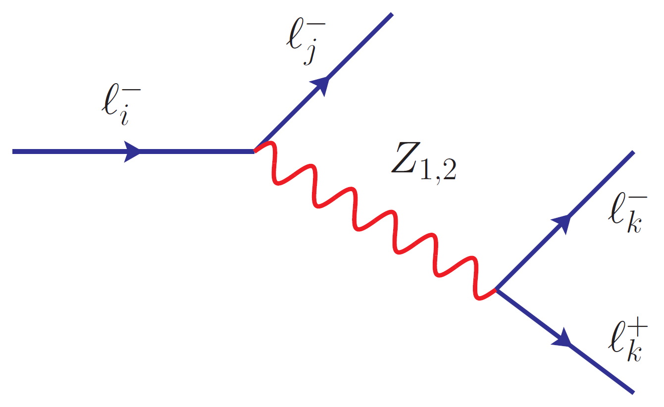
Figure 1: Tree-level diagram for $\mu\rightarrow 3e$.

The $(1+\delta_{ij})$ factor takes care of identical particles in the final state. The constraints on the off-diagonal couplings of neutral bosons to charged fermions are given in Table IV.

Process	Exp. Bound	Constraint
$\mu^{-}\rightarrow e^{-}e^{+}e^{-}$	$<1.0\times 10^{-12}$	$|(V_{L_{l}}\mathcal{Y}_{E}\mathcal{Y}_{E}^{\dagger}V_{L_{l}}^{\dagger})_{e\mu}|<4.66\times 10^{-5}(\frac{M_{L}}{0.7\text{ TeV}})^{2}$
$\tau^{-}\rightarrow e^{-}e^{+}e^{-}$	$<2.7\times 10^{-8}$	$|(V_{L_{l}}\mathcal{Y}_{E}\mathcal{Y}_{E}^{\dagger}V_{L_{l}}^{\dagger})_{e\tau}|<1.81\times 10^{-2}(\frac{M_{L}}{0.7\text{ TeV}})^{2}$
$\tau^{-}\rightarrow e^{-}\mu^{+}\mu^{-}$	$<2.7\times 10^{-8}$	$|(V_{L_{l}}\mathcal{Y}_{E}\mathcal{Y}_{E}^{\dagger}V_{L_{l}}^{\dagger})_{e\tau}|<1.28\times 10^{-2}(\frac{M_{L}}{0.7\text{ TeV}})^{2}$
$\tau^{-}\rightarrow\mu^{-}e^{+}e^{-}$	$<1.8\times 10^{-8}$	$|(V_{L_{l}}\mathcal{Y}_{E}\mathcal{Y}_{E}^{\dagger}V_{L_{l}}^{\dagger})_{\mu\tau}|<1.05\times 10^{-2}(\frac{M_{L}}{0.7\text{ TeV}})^{2}$
$\tau^{-}\rightarrow\mu^{-}\mu^{+}\mu^{-}$	$<2.1\times 10^{-8}$	$|(V_{L_{l}}\mathcal{Y}_{E}\mathcal{Y}_{E}^{\dagger}V_{L_{l}}^{\dagger})_{\mu\tau}|<1.60\times 10^{-2}(\frac{M_{L}}{0.7\text{ TeV}})^{2}$

Table IV: Constraints from three body decays of charged leptons. New contributions to diagonal couplings are ignored in this analysis but the mixing between $Z_{1}$ and $Z_{2}$ are not omitted. The results are quoted as a function of vector-like lepton mass $M_{L}$ (TeV).

4.3 Radiative Decays of Charged Leptons

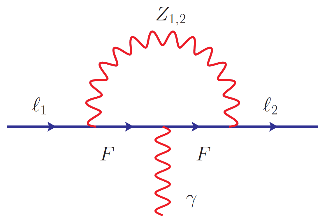
Figure 2: One-loop $\mu\to e\gamma$ mediated by neutral gauge bosons. $F$ stands for SM as well as vector-like charged leptons.

The radiative decays of the form $\ell_{1}\to\ell_{2}\gamma$ arise from one-loop diagrams as shown in Fig. 2 for $\mu\to e\gamma$. The gauge interaction leading to such decays with VL-lepton $F$ in the internal line is given by

$$\mathcal{L}_{gauge}=\sum_{j=1}^{2}\sum_{i=1}^{2}\overline{F}\gamma^{\mu}\left(\mathcal{C}_{L_{i}}^{Fj}P_{L}+\mathcal{C}_{R_{i}}^{Fj}P_{R}\right)\ell_{j}Z_{i_{\mu}}+\text{h.c.}.$$ (4.52)

The appropriate coefficients can be obtained from Eqs. (3.23), and (3.24) converted to the mass basis of neutral gauge bosons, imposing parity symmetry:

$$\mathcal{C}_{L_{1}}^{Fj}= \leavevmode\nobreak\ g_{L}\cos\theta_{W}\left(\sin\xi\frac{1}{2\sqrt{\cos 2\theta_{W}}}\frac{g_{Y}^{2}}{g_{L}^{2}}-\cos\xi\left(\frac{1}{2}+\frac{g_{Y}^{2}}{2g_{L}^{2}}\right)\rho_{L_{F}}V^{\dagger}_{L_{j}}\right),$$ (4.53)

$$\mathcal{C}_{R_{1}}^{Fj}= \leavevmode\nobreak\ g_{L}\cos\theta_{W}\left(\sin\xi\frac{1}{2\sqrt{\cos 2\theta_{W}}}\frac{\kappa_{R}}{\kappa_{L}}\rho_{L_{F}}V^{\dagger}_{L_{j}}\right),$$

$$\mathcal{C}_{L(R)_{2}}^{Fj}= -\mathcal{C}_{L(R)_{1}}^{Fj}(\xi\to\xi+\pi/2).$$

Process	Exp. Bound	Constraint
$\mu^{-}\rightarrow e^{-}\gamma$	$<4.2\times 10^{-13}$	$|(V_{L_{l}}\mathcal{Y}_{E}\mathcal{Y}_{E}^{\dagger}V_{L_{l}}^{\dagger})_{e\mu}|<1.18\times 10^{-6}(\frac{M_{L}}{0.7\text{ TeV}})^{2}$
$\tau^{-}\rightarrow e^{-}\gamma$	$<3.3\times 10^{-8}$	$|(V_{L_{l}}\mathcal{Y}_{E}\mathcal{Y}_{E}^{\dagger}V_{L_{l}}^{\dagger})_{e\tau}|<1.32\times 10^{-2}(\frac{M_{L}}{0.7\text{ TeV}})^{2}$
$\tau^{-}\rightarrow\mu^{-}\gamma$	$<4.4\times 10^{-8}$	$|(V_{L_{l}}\mathcal{Y}_{E}\mathcal{Y}_{E}^{\dagger}V_{L_{l}}^{\dagger})_{\mu\tau}|<1.78\times 10^{-2}(\frac{M_{L}}{0.7\text{ TeV}})^{2}$

Table V: Constraints from $\ell_{1}\to\ell_{2}\gamma$ processes. The vector-like lepton mass enhancement appearing in these diagrams is taken to be $=1.0$ TeV. The results are quoted as a function of vector-like lepton mass $M_{L}$(TeV).

The partial width for $\ell_{1}\to\ell_{2}\gamma$ is Lavoura:2003xp

$$\Gamma=\frac{(m_{1}^{2}-m_{2}^{2})^{3}}{16\pi m_{1}^{3}}\left(|\sigma_{L}|^{2}+|\sigma_{R}|^{2}\right).$$ (4.54)

Using the Eqs. (4.52) and (4.53), the coefficients $\sigma_{L,R}$ for $\mu\to e\gamma$ mediated by the VL-lepton $F$ are the following, where the subscript $i=1,2$ corresponds to $Z_{1,2}$:

$$\sigma_{L,R}=\sum_{i=1}^{2}\sigma_{L_{i},R_{i}},$$ (4.55)

where,

$$\sigma_{L_{i}}= -\left(\mathcal{C}_{R_{i}}^{eF}\mathcal{C}_{R_{i}}^{F\mu}y_{1}+\mathcal{C}_{L_{i}}^{eF}\mathcal{C}_{L_{i}}^{F\mu}y_{2}+\mathcal{C}_{R_{i}}^{eF}\mathcal{C}_{L_{i}}^{F\mu}y_{3}+\mathcal{C}_{L_{i}}^{eF}\mathcal{C}_{R_{i}}^{F\mu}y_{4}\right),$$ (4.56)

$$\sigma_{R_{i}}= -\left(\mathcal{C}_{R_{i}}^{eF}\mathcal{C}_{R_{i}}^{F\mu}y_{2}+\mathcal{C}_{L_{i}}^{eF}\mathcal{C}_{L_{i}}^{F\mu}y_{1}+\mathcal{C}_{R_{i}}^{eF}\mathcal{C}_{L_{i}}^{F\mu}y_{4}+\mathcal{C}_{L_{i}}^{eF}\mathcal{C}_{R_{i}}^{F\mu}y_{3}\right).$$

The factors $y_{i}$, with $c=\dfrac{i}{96m_{Z_{i}}^{2}(m_{Z_{i}}^{2}-m_{F}^{2})^{4}\pi^{2}}$, are

$$y_{1}= c\frac{m_{\mu}}{2}\Bigl{(}(m_{Z_{i}}^{2}-m_{F}^{2})\left\{-8m_{Z_{i}}^{6}+30m_{Z_{i}}^{4}m_{F}^{2}-9m_{Z_{i}}^{2}m_{F}^{4}+5m_{F}^{6}\right.$$ (4.57)

$$\left.+m_{e}^{2}(2m_{Z_{i}}^{4}+5m_{Z_{i}}^{2}m_{F}^{2}-mF^{4})\right\}+6m_{Z_{i}}^{4}m_{F}^{2}(m_{e}^{2}+3m_{F}^{2})\ln{\frac{m_{F}^{2}}{m_{Z_{i}}^{2}}}\Bigr{)},$$

$$y_{2}= y_{1}(m_{e}\leftrightarrow m_{\mu}),$$

$$y_{3}= c\frac{m_{F}}{2}\Bigl{(}(m_{Z_{i}}^{2}-m_{F}^{2})\left\{(m_{\mu}^{2}+m_{e}^{2})(m_{F}^{4}-2m_{Z_{i}}^{4}-5m_{Z_{i}}^{2}m_{F}^{2})+6(4m_{Z_{i}}^{6}-3m_{Z_{i}}^{4}m_{F}^{2}-m_{F}^{6})\right\}$$

$$-6m_{Z_{i}}^{4}m_{F}^{2}(m_{\mu}^{2}+m_{e}^{2}-6m_{Z_{i}}^{2}+6m_{F}^{2})\ln{\frac{m_{F}^{2}}{m_{Z_{i}}^{2}}}\Bigr{)},$$

$$y_{4}= -c\,m_{e}m_{\mu}m_{F}\left(11m_{Z_{i}}^{6}-18m_{Z_{i}}^{4}m_{F}^{2}+9m_{Z_{i}}^{2}m_{F}^{4}-2m_{F}^{6}+6m_{Z_{i}}^{6}\ln{\frac{m_{F}^{2}}{m_{Z_{i}}^{2}}}\right).$$

The dominant contribution to radiative decays arise from the chirally enhanced VL-lepton mediated diagrams. In obtaining the constraints, the mass of the mediator VLF is set to 1 TeV. The results are given in Table V.

4.4 Mass difference of Neutral Mesons

The effective Lagrangian for $\Delta F=2$ processes mediated by neutral gauge bosons, as shown in Fig. 3, is of the form

$$\mathcal{L}=\sum_{k=1}^{2}\left(C_{L_{k}}(\Lambda)\,\overline{q}_{L_{i}}^{\alpha}\gamma^{\mu}q_{L_{j}}^{\alpha}Z_{k_{\mu}}+C_{R_{k}}(\Lambda)\,\overline{q}_{R_{i}}^{\alpha}\gamma^{\mu}q_{R_{j}}^{\alpha}Z_{k_{\mu}}+\frac{1}{2}M^{2}_{Z_{k}}Z_{k_{\mu}}Z_{k}^{\mu}\right)$$ (4.58)

where i and j are flavor indices, Greek indices stand for color, and $C(\Lambda)$ are the coefficients at high-scale. Upon integrating out the $Z_{1}$ and $Z_{2}$ masses, the Lagrangian becomes

$$\mathcal{H}= \sum_{k=1}^{2}\frac{1}{2M^{2}_{Z_{k}}}\Bigl{(}C^{2}_{L_{k}}(\Lambda)\,\overline{q}_{L_{i}}^{\alpha}\gamma_{\mu}q_{L_{j}}^{\alpha}\,\overline{q}_{L_{i}}^{\beta}\gamma^{\mu}q_{L_{j}}^{\beta}+C_{R_{k}}^{2}(\Lambda)\,\overline{q}_{R_{i}}^{\alpha}\gamma_{\mu}q_{R_{j}}^{\alpha}\,\overline{q}_{R_{i}}^{\beta}\gamma^{\mu}q_{R_{j}}^{\beta}$$ (4.59)

$$\qquad\qquad\qquad+2C_{L_{k}}(\Lambda)\,C_{R_{k}}(\Lambda)\,\overline{q}_{L_{i}}^{\alpha}\gamma_{\mu}q_{L_{j}}^{\alpha}\,\overline{q}_{R_{i}}^{\beta}\gamma^{\mu}q_{R_{j}}^{\beta}\Bigr{)}.$$

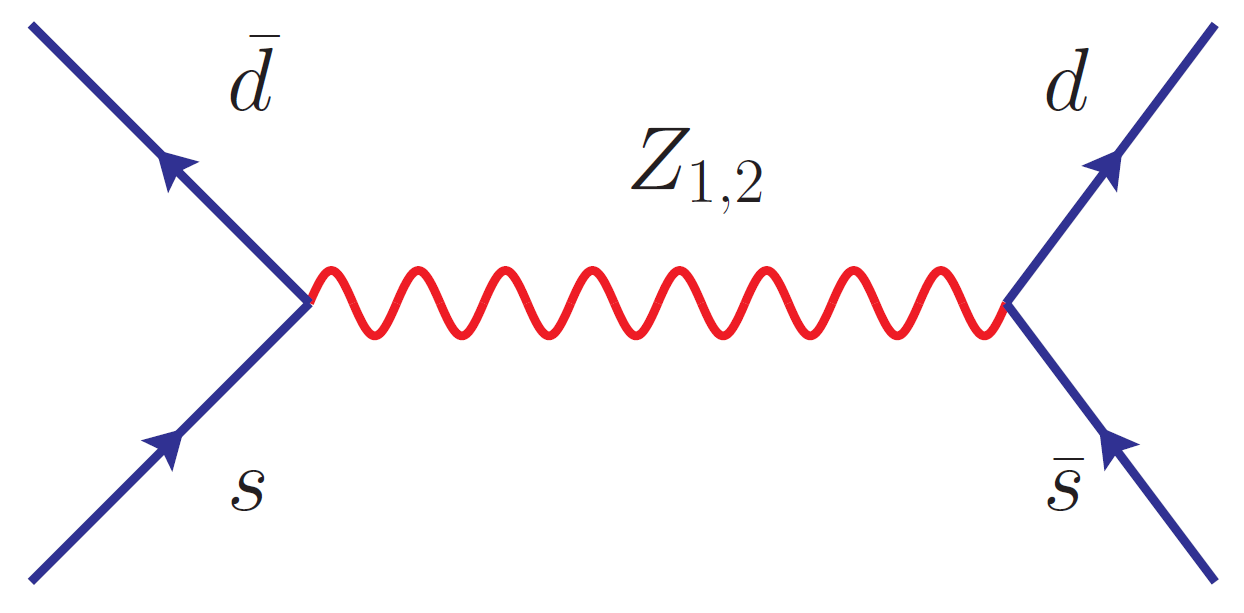
Figure 3: Tree-level diagram contributing to kaon mixing.

Process	$\Delta\text{M}_{\text{exp}}$(GeV)	$\Delta\text{M}_{\text{SM}}$	Constraint $(\frac{M_{F}}{1\text{ TeV}})^{2}$
$K-\overline{K}$	$(3.484\pm 0.006)\times 10^{-15}$	$2.364\times 10^{-15}$ GeV	$|(V_{L_{f}}\mathcal{Y}_{D}\mathcal{Y}_{D}^{\dagger}V_{L_{f}}^{\dagger})_{ds}|\leq 2.12\times 10^{-4}$
$D-\overline{D}$	$(6.2586^{+2.70}_{-2.90})\times 10^{-15}$	$3.87\times 10^{-15}$ GeV	$|(V_{L_{f}}\mathcal{Y}_{U}\mathcal{Y}_{U}^{\dagger}V_{L_{f}}^{\dagger})_{uc}|\leq 9.63\times 10^{-5}$
$B-\overline{B}$	$(3.334\pm 0.013)\times 10^{-13}$	$(0.543\pm 0.029)\text{ps}^{-1}$Lenz:2019lvd	$|(V_{L_{f}}\mathcal{Y}_{D}\mathcal{Y}_{D}^{\dagger}V_{L_{f}}^{\dagger})_{db}|\leq 3.76\times 10^{-4}$
$B_{s}-\overline{B}_{s}$	$(1.1688\pm 0.0014)\times 10^{-11}$	$(18.77\pm 0.86)\text{ps}^{-1}$Lenz:2019lvd	$|(V_{L_{f}}\mathcal{Y}_{D}\mathcal{Y}_{D}^{\dagger}V_{L_{f}}^{\dagger})_{sb}|\leq 4.35\times 10^{-4}$

Table VI: Constraints from neutral meson mass differences. The results are quoted as a function of vector-like quark mass $M_{F}$ (TeV). $B_{q}-\overline{B_{q}}$ calculations are done using Eq. (4.64) while the other two are evaluated using Eq. (4.62). More details can be found in Appendix. B.

The mass difference can be evaluated as $\Delta M=2\text{Re}\bra{\phi}\mathcal{H}\ket{\overline{\phi}}$, $\phi$ being the meson state. In general, the NP operators contributing to $\Delta F=2$ processes are Bona:2007vz

$$\mathcal{O}_{1}^{\,q_{i}\,q_{j}} =\overline{q}_{Lj}^{\alpha}\gamma_{\mu}q_{Li}^{\alpha}\,\overline{q}_{Lj}^{\beta}\gamma^{\mu}q_{Li}^{\beta}\,,$$ (4.60)

$$\mathcal{O}_{2}^{\,q_{i}\,q_{j}} =\overline{q}_{Rj}^{\alpha}q_{Li}^{\alpha}\,\overline{q}_{Rj}^{\beta}q_{Li}^{\beta}\,,$$

$$\mathcal{O}_{3}^{\,q_{i}\,q_{j}} =\overline{q}_{Rj}^{\alpha}q_{Li}^{\beta}\,\overline{q}_{Rj}^{\beta}q_{Li}^{\alpha}\,,$$

$$\mathcal{O}_{4}^{\,q_{i}\,q_{j}} =\overline{q}_{Rj}^{\alpha}q_{Li}^{\alpha}\,\overline{q}_{Lj}^{\beta}q_{Ri}^{\beta}\,,$$

$$\mathcal{O}_{5}^{\,q_{i}\,q_{j}} =\overline{q}_{Rj}^{\alpha}q_{Li}^{\beta}\,\overline{q}_{Lj}^{\beta}q_{Ri}^{\alpha}\,,$$

and $\widetilde{\mathcal{O}}_{1,2,3}^{\,q_{i}\,q_{j}}$, obtained by the exchange $L\leftrightarrow R$. Using Eqs. (4.59) and (4.60), the effective Hamiltonian for meson mixing mass difference can be written as

$$\mathcal{H}_{\text{{eff}}}=C_{1}(M_{Z})\mathcal{O}_{1}+\widetilde{C}_{1}(M_{Z})\mathcal{\widetilde{O}}_{1}-4C_{5}(M_{Z})\mathcal{O}_{5}.$$ (4.61)

Here, the operator $\mathcal{O}_{5}$ is obtained by Fierz transformation Nishi:2004st of $\overline{q}_{Li}^{\alpha}\gamma_{\mu}q_{Lj}^{\alpha}\overline{q}_{Ri}^{\beta}\gamma^{\mu}q_{Rj}^{\beta}$ in Eq. (4.59). The Wilson coefficients (WCs) at $M_{Z_{1(2)}}$ scale (or any NP scale, $\Lambda$) need to be evolved down to hadronic scale $m_{b}=4.6$ GeV for bottom mesons, $\mu_{D}=2.8$ GeV for charmed mesons and $\mu_{K}=2$ GeV for Kaons, which are the renormalization scales used in lattice computation of matrix elements Bona:2007vz . Renormalization group evolution of $C_{5}$ induces $C_{4}$, causing the corresponding operator to appear in the expression of $\Delta M$ at the hadronic scale. This is given by the analytical formula:

$$\bra{\overline{\phi}}\mathcal{H}_{\text{eff}}\ket{\phi}_{i}=\sum_{j=1}^{5}\sum_{r=1}^{5}(b_{j}^{(r,i)}+\eta c_{j}^{(r,i)})\eta^{a_{j}}C_{i}(\Lambda))\bra{\overline{\phi}}\mathcal{Q}_{r}\ket{\phi},$$ (4.62)

where, $\eta=\alpha_{s}(\Lambda)/\alpha_{s}(m_{t})$, and $a_{j}$, $b_{j}^{(r,i)}$ and $c_{j}^{(r,i)}$ are the magic numbers. The relevant constants and magic numbers are provided in Appendix. B.3.

We follow a different approach for obtaining the mass differences in the case of $B_{q}$-mesons DiLuzio:2019jyq ; He:2006bk , although the expression in Eq. (4.62) is equally valid. The SM predicts Buchalla:1995vs

$$\Delta M_{q}=\frac{2G_{F}^{2}}{4\pi^{2}}M_{W}^{2}\lambda_{q}^{2}\hat{\eta}_{B}S_{0}(x_{t})\frac{\langle\mathcal{O}_{1}\rangle}{2M_{B_{q}}},$$ (4.63)

where, $q=\{s,d\}$, $\lambda_{q}=V_{tb}V_{tq}^{*}$, $S_{0}$ is the Inami-Lim function Inami:1980fz , $x_{t}=(\overline{m}_{t}(\overline{m}_{t})/M_{W})^{2}$, $\hat{\eta}_{B}=0.84$ and $\langle\mathcal{O}_{1}\rangle=\frac{2}{3}M_{B_{q}}^{2}f^{2}_{b_{q}}B_{1}(m_{b})$. Using this, the SM+NP contribution to mass mixing normalized to the SM one is given by

$$\frac{\Delta M_{q}^{\text{SM+NP}}}{\Delta M_{q}^{\text{SM}}}= \bigg{|}1+\frac{\sqrt{2}G_{F}M_{Z_{1}}^{2}}{\mathtt{C}^{\Delta_{SM}}}\sum_{k=1,2}\bigg{[}\frac{2}{3}\bigg{(}\frac{\widetilde{C}_{L_{k}}^{{ij}^{2}}+\widetilde{C}_{R_{k}}^{{ij}^{2}}}{M_{Z_{k}}^{2}}\eta_{k}^{6/23}\bigg{)}$$ (4.64)

$$-\frac{B_{5}}{B_{1}}\bigg{(}\frac{2M^{2}_{B_{q}}}{3(m_{b}+m_{q})^{2}}+1\bigg{)}\bigg{(}\frac{\widetilde{C}_{L_{k}}^{ij}\widetilde{C}_{R_{k}}^{ij}}{M_{Z_{k}}^{2}}\eta_{k}^{3/23}\bigg{)}$$

$$+\frac{1}{3}\frac{B_{4}}{B_{1}}\bigg{(}\frac{2M^{2}_{B_{q}}}{(m_{b}+m_{q})^{2}}+\frac{1}{3}\bigg{)}\bigg{(}\frac{\widetilde{C}_{L_{k}}^{ij}\widetilde{C}_{R_{k}}^{ij}}{M_{Z_{k}}^{2}}\left(\eta_{k}^{3/23}-\eta_{k}^{-24/23}\right)\bigg{)}\bigg{]}\bigg{|},$$

with $\mathtt{C}^{\Delta_{\text{SM}}}=\frac{G_{F}^{2}}{12\pi}\lambda_{q}^{2}M_{W}^{2}S_{0}(x_{t})\hat{\eta}_{B}$. The analysis for $B_{q}$ mixings is done with a $2\,\sigma$ deviation in the SM predictions and $1\,\sigma$ in experimental measurements while $2\,\sigma$ deviation in the experimental measurements is allowed for $K$ and $D$ mass differences. The constraints obtained are tabulated in Table VI along with the experimental bounds and the SM predictions used.

4.5 Charged Leptonic Decays of Mesons

Neutral mesons decaying to charged leptons of the form $\phi\to\ell_{i}^{+}\ell_{i}^{-}$ are analyzed here, where $\phi$ represents meson and $\ell$ stands for lepton. The decay rate, with $f_{\phi}$ being the form factor, is given by

$$\Gamma=\frac{g_{L}^{4}}{32\pi\cos^{4}\theta_{W}}f_{\phi}^{2}m_{\ell}^{2}m_{\phi}\sqrt{1-\frac{4m_{\ell}^{2}}{m_{\phi}^{2}}}(|\mathcal{C}_{L}|^{2}+|\mathcal{C}_{R}|^{2}),$$ (4.65)

where, $\mathcal{C}_{X}=\dfrac{C_{X_{1}}^{\ell\ell}}{M_{Z_{1}}^{2}}(\widetilde{C}_{L_{1}}^{ij}-\widetilde{C}_{R_{1}}^{ij})+\dfrac{C_{X_{2}}^{\ell\ell}}{M_{Z_{2}}^{2}}(\widetilde{C}_{L_{2}}^{ij}-\widetilde{C}_{R_{2}}^{ij}),\text{ and }X=\{L,R\}.$

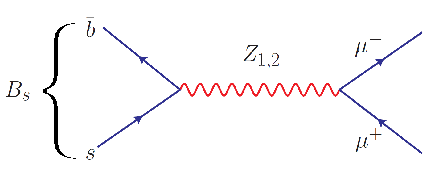
Figure 4: Tree-level diagram for $B_{s}\to\mu^{+}\mu^{-}$.

The new contributions to $Z_{i}\,\overline{\ell}\ell$ couplings are ignored; i.e., $R_{\ell\ell}=0$ and the allowed parameter space of $R_{ij}$ from the quark sector is determined. For $B_{q}\to\mu^{+}\mu^{-}$ decays, the constraints are obtained for the central value of the experimental measurements. The constraints obtained are listed in Table VII along with the experimental bounds and the form factors used. We see that the constraints are small when electrons are the final particles owing to the small mass while muon final states give stronger constraints on account of the stringent experimental bounds.

Process	Exp. Bound	Constraint	$f_{\phi}$ (GeV)Melikhov:2000yu
$D\rightarrow e^{+}e^{-}$	$<7.9\times 10^{-8}$	$|(V_{L_{f}}\mathcal{Y}_{U}\mathcal{Y}_{U}^{\dagger}V_{L_{f}}^{\dagger})_{uc}|<35.96(\frac{M_{F}}{1\text{ TeV}})^{2}$	$0.200$
$D\rightarrow\mu^{+}\mu^{-}$	$<6.2\times 10^{-9}$	$|(V_{L_{f}}\mathcal{Y}_{U}\mathcal{Y}_{U}^{\dagger}V_{L_{f}}^{\dagger})_{uc}|<4.88\times 10^{-2}(\frac{M_{F}}{1\text{ TeV}})^{2}$	$0.200$
$B\rightarrow e^{+}e^{-}$	$<8.3\times 10^{-8}$	$|(V_{L_{f}}\mathcal{Y}_{D}\mathcal{Y}_{D}^{\dagger}V_{L_{f}}^{\dagger})_{bd}|<12.70(\frac{M_{F}}{1\text{ TeV}})^{2}$	$0.180$
$B\rightarrow\mu^{+}\mu^{-}$	$(1.1^{+1.4}_{-1.3})\times 10^{-10}$	$|(V_{L_{f}}\mathcal{Y}_{D}\mathcal{Y}_{D}^{\dagger}V_{L_{f}}^{\dagger})_{bd}|\leq 2.24\times 10^{-3}(\frac{M_{F}}{1\text{ TeV}})^{2}$	$0.180$
$B\rightarrow\tau^{+}\tau^{-}$	$<2.1\times 10^{-3}$	$|(V_{L_{f}}\mathcal{Y}_{D}\mathcal{Y}_{D}^{\dagger}V_{L_{f}}^{\dagger})_{bd}|<0.676(\frac{M_{F}}{1\text{ TeV}})^{2}$	$0.180$
$B_{s}\rightarrow e^{+}e^{-}$	$<2.8\times 10^{-7}$	$|(V_{L_{f}}\mathcal{Y}_{D}\mathcal{Y}_{D}^{\dagger}V_{L_{f}}^{\dagger})_{bs}|<20.92(\frac{M_{F}}{1\text{ TeV}})^{2}$	$0.200$
$B_{s}\rightarrow\mu^{+}\mu^{-}$	$3.0\pm 0.4\times 10^{-9}$	$|(V_{L_{f}}\mathcal{Y}_{D}\mathcal{Y}_{D}^{\dagger}V_{L_{f}}^{\dagger})_{bs}|\leq 1.05\times 10^{-2}(\frac{M_{F}}{1\text{ TeV}})^{2}$	$0.200$
$B_{s}\rightarrow\tau^{+}\tau^{-}$	$<6.8\times 10^{-3}$	$|(V_{L_{f}}\mathcal{Y}_{D}\mathcal{Y}_{D}^{\dagger}V_{L_{f}}^{\dagger})_{bs}|<1.08(\frac{M_{F}}{1\text{ TeV}})^{2}$	$0.200$

Table VII: Constraints from flavor conserving charged leptonic decays of neutral mesons. The results are quoted as a function of vector-like quark mass $M_{F}$.

4.6 Semi-Leptonic Meson Decay

Here, we explore the tree-level lepton flavor conserving decays of mesons of the for $\phi_{H}\to phi_{L}\ell^{+}\ell^{-}$. We assume that total decay width is comprised of only the tree-level contribution from the NP model parameters, so the results are less constraining than what would be obtained with a more thorough investigation including the SM interference terms. The decay width for such processes is given by

$$\Gamma=\frac{g^{4}_{L}}{64\pi^{3}\cos^{4}\theta_{W}m_{H}}|f_{+}(0)|^{2}\mathcal{F}\,(|\mathcal{C}_{L}|^{2}+|\mathcal{C}_{R}|^{2}),$$ (4.66)

where, $\mathcal{F}=\dfrac{m_{V}^{2}}{48m_{H}^{2}}\left(-2m_{H}^{6}+9m_{H}^{4}m_{V}^{2}-6m_{H}^{2}m_{V}^{4}-6(m_{V}^{3}-m_{H}^{2}m_{V})^{2}\ln{\frac{m_{V}^{2}-m_{H}^{2}}{m_{V}^{2}}}\right)$, $m_{H}$ is the parent meson mass and $m_{V}$ is the corresponding vector meson mass. The input parameters used are given in Appendix. C. The coefficients $\mathcal{C}_{L,R}$ are given by

$$\mathcal{C}_{X}=\frac{C_{X_{1}}^{\ell\ell}(\widetilde{C}_{L_{1}}^{ij}+\widetilde{C}_{R_{1}}^{ij})}{M_{Z_{1}}^{2}}+\frac{C_{X_{2}}^{l\ell\ell}(\widetilde{C}_{L_{2}}^{ij}+\widetilde{C}_{R_{2}}^{ij})}{M_{Z_{2}}^{2}},\quad X=\{L,R\}.$$ (4.67)

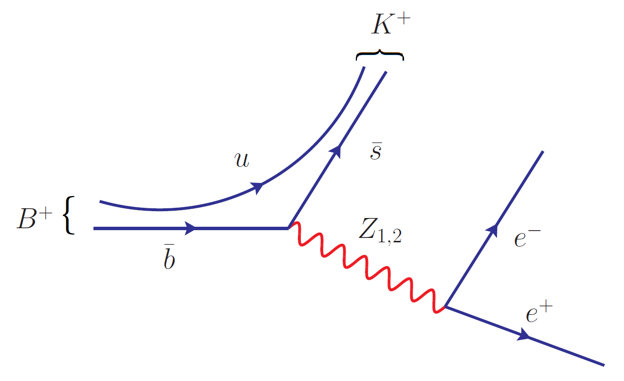
Figure 5: Tree-level diagram for $B^{+}\to K^{+}e^{+}e^{-}$.

Process	Exp. Bound	Constraint
$K^{+}\to\pi^{+}e^{+}e^{-}$	$(3\pm 0.09)\times 10^{-7}$	$|(V_{L_{f}}\mathcal{Y}_{D}\mathcal{Y}_{D}^{\dagger}V_{L_{f}}^{\dagger})_{sd}|\leq 3.83\times 10^{-2}(\frac{M_{F}}{1\text{ TeV}})^{2}$
$K^{+}\to\pi^{+}\mu^{+}\mu^{-}$	$(9.4\pm 0.6)\times 10^{-8}$	$|(V_{L_{f}}\mathcal{Y}_{D}\mathcal{Y}_{D}^{\dagger}V_{L_{f}}^{\dagger})_{sd}|\leq 2.15\times 10^{-2}(\frac{M_{F}}{1\text{ TeV}})^{2}$
$K^{+}\to\pi^{+}\nu\overline{\nu}$	$(1.7\pm 1.1)\times 10^{-10}$	$|(V_{L_{f}}\mathcal{Y}_{D}\mathcal{Y}_{D}^{\dagger}V_{L_{f}}^{\dagger})_{sd}|\leq 3.66\times 10^{-4}(\frac{M_{F}}{1\text{ TeV}})^{2}$
$B^{+}\to\pi^{+}\ell^{+}\ell^{-}$	$<4.9\times 10^{-8}$	$|(V_{L_{f}}\mathcal{Y}_{D}\mathcal{Y}_{D}^{\dagger}V_{L_{f}}^{\dagger})_{bd}|<6.49\times 10^{-3}(\frac{M_{F}}{1\text{ TeV}})^{2}$
$B^{+}\to\pi^{+}e^{+}e^{-}$	$<8.0\times 10^{-8}$	$|(V_{L_{f}}\mathcal{Y}_{D}\mathcal{Y}_{D}^{\dagger}V_{L_{f}}^{\dagger})_{bd}|<1.18\times 10^{-2}(\frac{M_{F}}{1\text{ TeV}})^{2}$
$B^{+}\to\pi^{+}\mu^{+}\mu^{-}$	$(1.75\pm 0.22)\times 10^{-8}$	$|(V_{L_{f}}\mathcal{Y}_{D}\mathcal{Y}_{D}^{\dagger}V_{L_{f}}^{\dagger})_{bd}|\leq 5.51\times 10^{-3}(\frac{M_{F}}{1\text{ TeV}})^{2}$
$B\to\pi\ell^{+}\ell^{-}$	$<5.3\times 10^{-8}$	$|(V_{L_{f}}\mathcal{Y}_{D}\mathcal{Y}_{D}^{\dagger}V_{L_{f}}^{\dagger})_{bd}|<9.6\times 10^{-3}(\frac{M_{F}}{1\text{ TeV}})^{2}$
$B\to\pi e^{+}e^{-}$	$8.4\times 10^{-8}$	$|(V_{L_{f}}\mathcal{Y}_{D}\mathcal{Y}_{D}^{\dagger}V_{L_{f}}^{\dagger})_{bd}|<1.71\times 10^{-2}(\frac{M_{F}}{1\text{ TeV}})^{2}$
$B\to\pi\mu^{+}\mu^{-}$	$<6.9\times 10^{-8}$	$|(V_{L_{f}}\mathcal{Y}_{D}\mathcal{Y}_{D}^{\dagger}V_{L_{f}}^{\dagger})_{bd}|<1.55\times 10^{-2}(\frac{M_{F}}{1\text{ TeV}})^{2}$
$B^{+}\to\pi^{+}\nu\overline{\nu}$	$<1.4\times 10^{-5}$	$|(V_{L_{f}}\mathcal{Y}_{D}\mathcal{Y}_{D}^{\dagger}V_{L_{f}}^{\dagger})_{bd}|<6.24\times 10^{-2}(\frac{M_{F}}{1\text{ TeV}})^{2}$
$B\to\pi\nu\overline{\nu}$	$<9\times 10^{-6}$	$|(V_{L_{f}}\mathcal{Y}_{D}\mathcal{Y}_{D}^{\dagger}V_{L_{f}}^{\dagger})_{bd}|<7.06\times 10^{-2}(\frac{M_{F}}{1\text{ TeV}})^{2}$
$B^{+}\to K^{+}\ell^{+}\ell^{-}$	$(4.51\pm 0.23)\times 10^{-7}$	$|(V_{L_{f}}\mathcal{Y}_{D}\mathcal{Y}_{D}^{\dagger}V_{L_{f}}^{\dagger})_{bs}|\leq 1.63\times 10^{-2}(\frac{M_{F}}{1\text{ TeV}})^{2}$
$B^{+}\to K^{+}e^{+}e^{-}$	$(5.5\pm 0.7)\times 10^{-7}$	$|(V_{L_{f}}\mathcal{Y}_{D}\mathcal{Y}_{D}^{\dagger}V_{L_{f}}^{\dagger})_{bs}|\leq 2.55\times 10^{-2}(\frac{M_{F}}{1\text{ TeV}})^{2}$
$B^{+}\to K^{+}\mu^{+}\mu^{-}$	$(4.41\pm 0.22)\times 10^{-7}$	$|(V_{L_{f}}\mathcal{Y}_{D}\mathcal{Y}_{D}^{\dagger}V_{L_{f}}^{\dagger})_{bs}|\leq 2.29\times 10^{-2}(\frac{M_{F}}{1\text{ TeV}})^{2}$
$B^{+}\to K^{+}\tau^{+}\tau^{-}$	$<2.25\times 10^{-3}$	$|(V_{L_{f}}\mathcal{Y}_{D}\mathcal{Y}_{D}^{\dagger}V_{L_{f}}^{\dagger})_{bs}|<1.63(\frac{M_{F}}{1\text{ TeV}})^{2}$
$B\to K\ell^{+}\ell^{-}$	$(3.1^{+0.8}_{-0.7})\times 10^{-7}$	$|(V_{L_{f}}\mathcal{Y}_{D}\mathcal{Y}_{D}^{\dagger}V_{L_{f}}^{\dagger})_{bs}|\leq 1.36\times 10^{-2}(\frac{M_{F}}{1\text{ TeV}})^{2}$
$B\to Ke^{+}e^{-}$	$(1.6^{+1.0}_{-0.8})\times 10^{-7}$	$|(V_{L_{f}}\mathcal{Y}_{D}\mathcal{Y}_{D}^{\dagger}V_{L_{f}}^{\dagger})_{bs}|\leq 1.38\times 10^{-2}(\frac{M_{F}}{1\text{ TeV}})^{2}$
$B\to K\mu^{+}\mu^{-}$	$(3.39\pm 0.34)\times 10^{-7}$	$|(V_{L_{f}}\mathcal{Y}_{D}\mathcal{Y}_{D}^{\dagger}V_{L_{f}}^{\dagger})_{bs}|\leq 2.00\times 10^{-2}(\frac{M_{F}}{1\text{ TeV}})^{2}$
$B^{+}\to K^{+}\nu\overline{\nu}$	$<1.6\times 10^{-5}$	$|(V_{L_{f}}\mathcal{Y}_{D}\mathcal{Y}_{D}^{\dagger}V_{L_{f}}^{\dagger})_{bs}|<5.51\times 10^{-2}(\frac{M_{F}}{1\text{ TeV}})^{2}$
$B\to K\nu\overline{\nu}$	$<2.6\times 10^{-5}$	$|(V_{L_{f}}\mathcal{Y}_{D}\mathcal{Y}_{D}^{\dagger}V_{L_{f}}^{\dagger})_{bs}|<7.03\times 10^{-2}(\frac{M_{F}}{1\text{ TeV}})^{2}$
$D^{+}\to\pi^{+}e^{+}e^{-}$	$<1.1\times 10^{-6}$	$|(V_{L_{f}}\mathcal{Y}_{U}\mathcal{Y}_{U}^{\dagger}V_{L_{f}}^{\dagger})_{uc}|<0.33(\frac{M_{F}}{1\text{ TeV}})^{2}$
$D^{+}\to\pi^{+}\mu^{+}\mu^{-}$	$<7.3\times 10^{-8}$	$|(V_{L_{f}}\mathcal{Y}_{U}\mathcal{Y}_{U}^{\dagger}V_{L_{f}}^{\dagger})_{uc}|<8.54\times 10^{-2}(\frac{M_{F}}{1\text{ TeV}})^{2}$
$D\to\pi e^{+}e^{-}$	$<4\times 10^{-6}$	$|(V_{L_{f}}\mathcal{Y}_{U}\mathcal{Y}_{U}^{\dagger}V_{L_{f}}^{\dagger})_{uc}|<1.44(\frac{M_{F}}{1\text{ TeV}})^{2}$
$D\to\pi\mu^{+}\mu^{-}$	$<1.8\times 10^{-4}$	$|(V_{L_{f}}\mathcal{Y}_{U}\mathcal{Y}_{U}^{\dagger}V_{L_{f}}^{\dagger})_{uc}|<9.67(\frac{M_{F}}{1\text{ TeV}})^{2}$
$D_{s}\to K^{+}\mu^{+}\mu^{-}$	$<2.1\times 10^{-5}$	$|(V_{L_{f}}\mathcal{Y}_{U}\mathcal{Y}_{U}^{\dagger}V_{L_{f}}^{\dagger})_{uc}|<1.67(\frac{M_{F}}{1\text{ TeV}})^{2}$
$D_{s}\to K^{+}e^{+}e^{-}$	$<3.7\times 10^{-6}$	$|(V_{L_{f}}\mathcal{Y}_{U}\mathcal{Y}_{U}^{\dagger}V_{L_{f}}^{\dagger})_{uc}|<0.99(\frac{M_{F}}{1\text{ TeV}})^{2}$

Table VIII: Constraints from flavor conserving charged leptonic decays of heavy mesons, quoted as a function of vector-like quark mass $M_{F}$.

The NP contribution to diagonal couplings from the lepton sector is set to zero since the quark vertex has the leading contribution. When the final state particles involve neutrinos, only the SM neutrino vertex is taken into account so that the $C_{X_{2}}$ coefficients vanish and the three flavors of neutrinos are summed together. As in the previous section, the constraints are obtained for the central values of the experimental measurements. They are tabulated in Table VIII.

5 Constraints on Charged Current Couplings

In this section, we find the constraints on the theory parameters modifying the charged current couplings. The major constraints arise from lepton flavor universality violating processes. We also look at $W_{L}$ decay to leptons and $\ell_{1}\to\ell_{2}\gamma$ processes. For simplicity, the part of Eq. (3.42) relevant to the processes being studied is rewritten as

$$-\mathcal{L}_{W_{L}}=\overline{\nu}_{L}\gamma^{\mu}W^{+}_{L\mu}\frac{g_{L}}{\sqrt{2}}(1-f_{\nu\ell})\ell_{L}+...+\text{h.c.}.$$ (5.68)

5.1 $W_{L}$ Decay to Leptons

Process	Exp. Bound	Constraint
$W_{L}^{+}\rightarrow e^{+}\nu$	$(10.71\pm 0.16)\%$	$-7.03\times 10^{-3}\leq f_{\nu e}\leq 2.61\times 10^{-2}$
$W_{L}^{+}\rightarrow\mu^{+}\nu$	$(10.63\pm 0.15)\%$	$-1.89\times 10^{-3}\leq f_{\nu\mu}\leq 2.93\times 10^{-2}$
$W_{L}^{+}\rightarrow\tau^{+}\nu$	$(11.38\pm 0.21)\%$	$-3.46\times 10^{-2}\leq f_{\nu\tau}\leq 7.67\times 10^{-3}$

Table IX: Constraints from leptonic decays of $W_{L}$. $f$’s are the new contribution to the charged current couplings as defined in Eq. (5.68). A $2\,\sigma$ deviation is allowed in obtaining the constraints.

Here, we obtain the constraints on the coupling of $W_{L}$ to leptons by studying its different decay modes. The decay rate of such processes is given by

$$\Gamma=\frac{g_{L}^{2}M_{W}}{48\pi}|1-f_{\nu\ell}|^{2}.$$ (5.69)

To accommodate the deviation in the total decay width of $W_{L}$ due to NP contribution, the branching ratio is computed by turning on the relevant coupling in each case. Since $\Gamma(W_{L}\to q_{i}q_{j})_{\text{SM}}=6\Gamma(W_{L}\to\nu_{\ell}\ell)_{\text{SM}}$ owing to the apparent unitarity of the CKM matrix, the total decay width of $W_{L}$ maybe written as

$$\Gamma_{W_{L}}=8\Gamma(W_{L}\to\nu_{\ell}\ell)_{\text{SM}}+\frac{g_{L}^{2}M_{W}}{48\pi}|1-f_{\nu\ell}|^{2}.$$ (5.70)

Then, the branching ratio of $W_{L}^{+}\to e^{+}\nu$, for example, would be $\Gamma(f_{\nu\ell}=f_{\nu e})/\Gamma_{W_{L}}(f_{\nu\ell}=f_{\nu e})$. We allow a $2\,\sigma$ deviation above and below the central value in obtaining the constraints. The constraints from $W_{L}$ decays are given in Table IX.

5.2 Radiative Decays of Charged Leptons

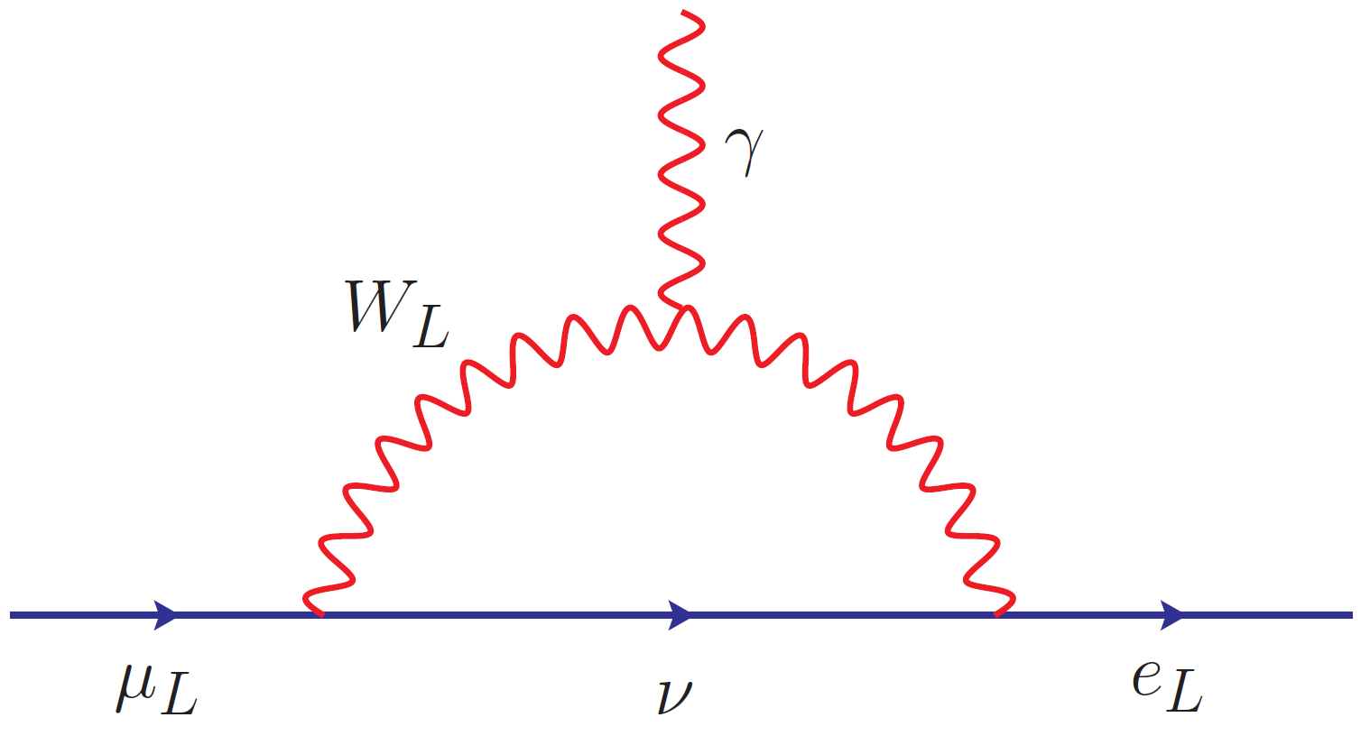
Figure 6: One-loop diagram of $\mu\to e\gamma$ mediated by $W_{L}$. Keeping one of the vertices to be SM-like will eliminate $\nu_{\tau}$ from appearing in this process.

Since the charged current couplings can be flavor-changing in this model, $\ell_{1}\to\ell_{2}\gamma$ processes can occur at one-loop level without a neutrino mass insertion in the internal fermion line. The gauge interaction relevant for the decay is

$$\mathcal{L}=\frac{g_{L}}{\sqrt{2}}\overline{e}\gamma^{\sigma}W_{L\sigma}^{-}\nu_{e}+\frac{g_{L}}{\sqrt{2}}\overline{\mu}\gamma^{\sigma}W_{L\sigma}^{-}\nu_{\mu}+\frac{g_{L}}{\sqrt{2}}f_{e\nu_{\mu}}\overline{e}\gamma^{\sigma}W_{L\sigma}^{-}\nu_{\mu}+\frac{g_{L}}{\sqrt{2}}f_{\mu\nu_{e}}\overline{\mu}\gamma^{\sigma}W_{L\sigma}^{-}\nu_{e}+...+\text{h.c.}$$ (5.71)

and the decay rate is computed along the same lines as Sec. 4.3. The internal fermion mediators are considered to be SM neutrinos such that one of the vertices is a SM vertex. The constraints from these processes are listed in Table X.

Process	Exp. Bound	Constraint
$\mu^{-}\rightarrow e^{-}\gamma$	$<4.2\times 10^{-13}$	$|f_{e\nu}+f_{\mu\nu}^{*}|<2.59\times 10^{-6}$
$\tau^{-}\rightarrow e^{-}\gamma$	$<3.3\times 10^{-8}$	$|f_{e\nu}+f_{\tau\nu}^{*}|<1.73\times 10^{-3}$
$\tau^{-}\rightarrow\mu^{-}\gamma$	$<4.4\times 10^{-8}$	$|f_{\mu\nu}+f_{\tau\nu}^{*}|<2.0\times 10^{-3}$

Table X: Constraints from $l_{1}\to l_{2}\gamma$ processes. The $f$’s are the new contributions to charged current interaction.

5.3 Lepton Flavour Universality Tests

In this section, we have analyzed the constraints arising from various lepton flavor universality (LFU) tests involving charged current. The ratio of leptonic decays of $W$ boson, predicted to be unity in the SM, can be a direct test of lepton universality. The theoretical uncertainties for these processes appear from the mass of the final state particles, which are small compared to the experimental uncertainties. Other theory parameters cancel out in the ratio. Using Eq. (5.69), the decay rate ratios given in Table XI take the form $1-2(f_{\nu\ell_{i}}-f_{\nu\ell_{j}})$ to the first order in both the parameters, where, $i$ is lepton flavor in the numerator, and $j$ is the one in the denominator. This formula is also valid for $\Gamma(K\to\pi\mu\nu)/\Gamma(K\to\pi e\nu)$, and for $\Gamma(\tau^{-}\to\mu^{-}\overline{\nu}_{\mu}\nu_{\tau})/\Gamma(\tau^{-}\to e^{-}\overline{\nu}_{e}\nu_{\tau})$ which is given in Table XIII.

Process	Exp. Bound	Constraint
$\Gamma(W_{L}\to\mu\nu)/\Gamma(W_{L}\to e\nu)$	$(0.996\pm 0.008)$	$-0.006\leq f_{\nu\mu}-f_{\nu e}\leq 0.010$
$\Gamma(W_{L}\to\tau\nu)/\Gamma(W_{L}\to e\nu)$	$(1.043\pm 0.024)$	$-0.046\leq f_{\nu\tau}-f_{\nu e}\leq 0.003$
$\Gamma(W_{L}\to\tau\nu)/\Gamma(W_{L}\to\mu\nu)$	$(1.070\pm 0.026)$	$-0.061\leq f_{\nu\tau}-f_{\nu\mu}\leq-0.009$
$\Gamma(K\to\pi\mu\nu)/\Gamma(K\to\pi e\nu)$	$(0.6608\pm 0.003)$	$0.167\leq f_{\nu\mu}-f_{\nu e}\leq 0.173$

Table XI: Lepton flavor universality violation in $W$ decays and semileptonic decay of K-meson. The $f$’s are the new contributions to charged current interactions. A $2\,\sigma$ deviation is allowed for obtaining the constraints.

Another set of LFU-violating constraints come from the purely leptonic decays of charged mesons. The ratios of such decays will be of the form

$$R=\frac{(m_{i}^{3}-m_{i}m_{\phi}^{2})^{2}\left(1-2(f_{\nu j}-f_{\nu i})\right)}{(m_{j}^{3}-m_{\phi}^{2}m_{j})^{2}}$$ (5.72)

where, $i$ is lepton in the numerator and $j$ is the one in the denominator. The constraints from these are given in Table XII. Yet another set of constraints come from the three-body decays of charged leptons. The theoretical prediction to the lowest order for

$$\frac{\Gamma(\tau^{-}\to e^{-}\overline{\nu}_{e}\nu_{\tau})}{\Gamma(\mu^{-}\to e^{-}\overline{\nu}_{e}\nu_{\mu})}=\frac{m_{\tau}^{2}}{m_{\mu}^{5}}\left(1-2(f_{\nu\tau}-f_{\nu\mu})\right).$$ (5.73)

Finally, we also look at ratios of the form $\Gamma(\tau\to M\nu_{\tau})/\Gamma(M\to\ell\nu_{\ell})$ which are given by

$$R_{\tau/M}=\frac{\Gamma(\tau\to M\nu_{\tau})}{\Gamma(M\to\ell\nu_{\ell})}=\frac{1}{2}\frac{m_{\tau}^{3}}{m_{M}m_{\ell}^{2}}\frac{(1-m_{M}^{2}/m_{\tau}^{2})^{2}}{(1-m_{\ell}^{2}/m_{M}^{2})^{2}}\left(1-2(f_{\nu\tau}-f_{\nu\ell})\right)\mbox{\cite[cite]{\@@bibref{Authors Phrase1YearPhrase2}{Decker:1993py}{\@@citephrase{(}}{\@@citephrase{)}}}}.$$ (5.74)

The results obtained from these sets of LFU-violating decays are given in Table XIII.

Process	Exp. Bound	Constraint
$\Gamma(K\to e\nu)/\Gamma(K\to\mu\nu)$	$(2.488\pm 0.009)\times 10^{-5}$	$-0.019\leq f_{\nu\mu}-f_{\nu e}\leq-0.012$
$\Gamma(\pi\to e\nu)/\Gamma(\pi\to\mu\nu)$	$(1.23\pm 0.0023)\times 10^{-4}$	$-0.026\leq f_{\nu\mu}-f_{\nu e}\leq-0.019$
$\Gamma(D_{s}\to\tau\nu)/\Gamma(D_{s}\to\mu\nu)$	$(10.73\pm 0.69)$	$-0.12\leq f_{\nu\tau}-f_{\nu\mu}\leq 0.020$

Table XII: LFUV from leptonic decays of mesons. The $f$’s are the new contributions to charged current interaction.

Process	Exp. Bound	Constraint
$\frac{\displaystyle\Gamma(\tau^{-}\to\mu^{-}\overline{\nu}_{\mu}\nu_{\tau})}{\displaystyle\Gamma(\tau^{-}\to e^{-}\overline{\nu}_{e}\nu_{\tau})}$	$(0.9764\pm 0.003)$	$8.8\times 10^{-3}\leq f_{\nu\mu}-f_{\nu e}\leq 1.48\times 10^{-2}$
$\frac{\displaystyle\Gamma(\tau^{-}\to e^{-}\overline{\nu}_{e}\nu_{\tau})}{\displaystyle\Gamma(\mu^{-}\to e^{-}\overline{\nu}_{e}\nu_{\mu})}$	$(1.349\pm 0.004)$	$-4.42\times 10^{-3}\leq f_{\nu\tau}-f_{\nu\mu}\leq 1.52\times 10^{-3}$
$\frac{\displaystyle\Gamma(\tau^{+}\to\pi^{+}\nu_{\tau})}{\displaystyle\Gamma(\pi^{+}\to\mu^{+}\nu_{\mu})}$	$(9704\pm 56)$	$-3.07\times 10^{-3}\leq f_{\nu\tau}-f_{\nu\mu}\leq 8.41\times 10^{-3}$
$\frac{\displaystyle\Gamma(\tau^{+}\to\pi^{+}\nu_{\tau})}{\displaystyle\Gamma(\pi^{+}\to e^{+}\nu_{e})}$	$(7.89\pm 0.05)\times 10^{7}$	$-2.35\times 10^{-2}\leq f_{\nu\tau}-f_{\nu e}\leq 1.04\times 10^{-2}$
$\frac{\displaystyle\Gamma(\tau^{+}\to K^{+}\nu_{\tau})}{\displaystyle\Gamma(K^{+}\to e^{+}\nu_{e})}$	$(1.89\pm 0.03)\times 10^{7}$	$-2.41\times 10^{-2}\leq f_{\nu\tau}-f_{\nu e}\leq 8.13\times 10^{-3}$

Table XIII: Constraints from other LFUV processes. The $f$’s are the new contributions to charged current interaction.

It should be noted that some of the constraints listed in this section appear to disagree with (or exclude) SM. These correspond to the experimental measurements that are not consistent with the SM prediction within $2\,\sigma$ uncertainty, like in the case of $\Gamma(W_{L}\to\tau\nu)/\Gamma(W_{L}\to\mu\nu)$ in Table XI, which does not accept a vanishing NP parameter. Combining all such constraints, we also see that there is no common region of parameter space that can explain all the LFU violating processes simultaneously.

5.4 Mass Difference of Neutral Mesons

In SM, neutral meson mixing occurs at one-loop level through the familiar box diagram involving $W_{L}$ boson. The presence of $W_{R}$ boson and heavy vector-like quarks can have additional effects on these processes which can give significant constraints on the NP parameters including the mass of $W_{R}$. The diagrams contributing to kaon mixing are shown in Fig. 7. We only consider the first two diagrams since the contribution from the one with two $W_{R}$’s is extremely small.

The $W_{L}-W_{L}$ box diagram contributes Ecker:1985vv

$$\mathcal{H}_{LL}=\frac{G_{F}^{2}M_{L}^{2}}{4\pi^{2}}(\bar{d}\gamma^{\mu}P_{L}s)^{2}\sum_{i,j}\lambda_{i}^{LL}\lambda_{j}^{LL}\big{\{}(1+\frac{x_{i}x_{j}}{4})I_{2}(x_{i},x_{j};1)-2x_{i}x_{j}I_{1}(x_{1},x_{j};1)\big{\}}$$ (5.75)

while the contribution from $W_{L}-W_{R}$ diagram is

$$\mathcal{H}_{LR}=\frac{G_{F}^{2}M_{L}^{2}\beta}{2\pi^{2}}\bar{d}P_{L}s\,\bar{d}P_{R}s\sum_{i,j}\lambda_{i}^{LR}\lambda_{j}^{RL}\sqrt{x_{i}x_{j}}\big{\{}(4+\beta x_{i}x_{j})I_{1}(x_{i},x_{j};\beta)-(1+\beta)I_{2}(x_{1},x_{j};\beta)\big{\}}$$ (5.76)

where,

$$x_{i}=m_{i}^{2}/M_{L}^{2}, \qquad\qquad\beta=M_{L}^{2}/M_{R}^{2}$$ (5.77)

$$I_{1}(x_{i},x_{j};\beta)= \frac{x_{i}\ln{x_{i}}}{(1-x_{i})(1-x_{i}\beta)(x_{i}-x_{j})}+(i\leftrightarrow j)-\frac{\beta\ln{\beta}}{(1-\beta)(1-x_{i}\beta)(1-x_{j}\beta)},$$

$$I_{2}(x_{i},x_{j};\beta)= \frac{x_{i}^{2}\ln{x_{i}}}{(1-x_{i})(1-x_{i}\beta)(x_{i}-x_{j})}+(i\leftrightarrow j)-\frac{\ln{\beta}}{(1-\beta)(1-x_{i}\beta)(1-x_{j}\beta)}.$$

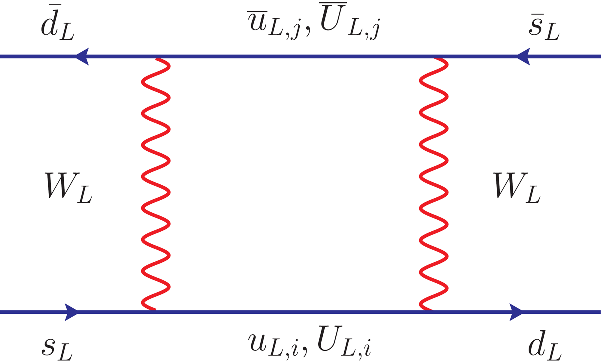
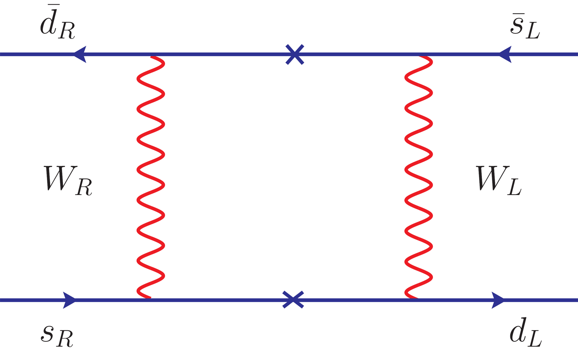
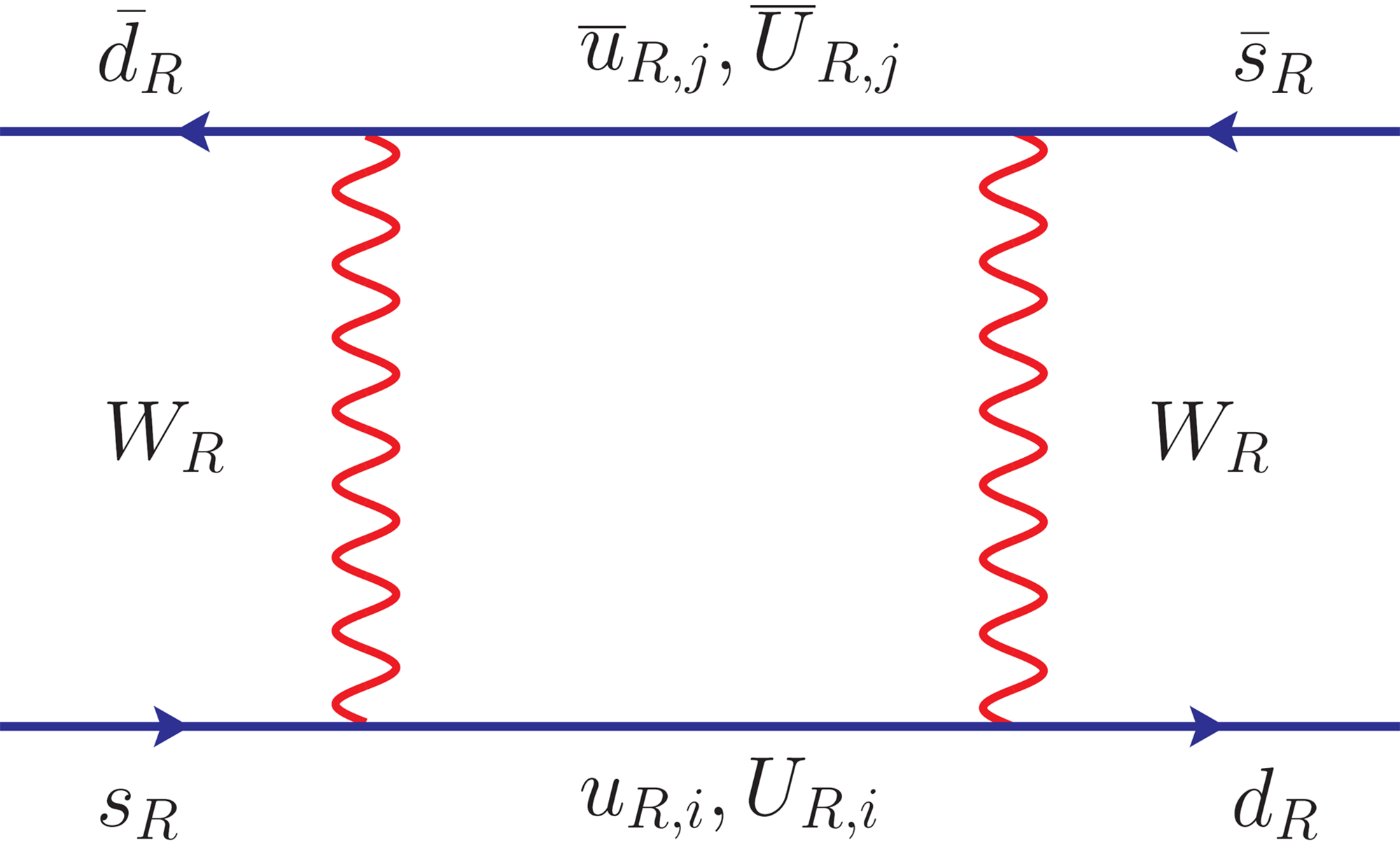
(a)                                        (b)                                          (c)

Figure 7: Box diagrams contributing to kaon mixing. The $F$ in the internal line represents both SM and vector-like up-type quarks. The last diagram is qualitatively insignificant compared to the other two.

In the above equations, we need to implement the GIM cancellation as well as the simplification $m_{u}\rightarrow 0$, and $m_{c}^{2}/M_{L,R}^{2}$ is kept to the first order Mohapatra:1983ae . The expressions for $\lambda_{i,j}$ are given in Appendix. D. Among the meson mixing processes, $K-\overline{K}$ gave significant constraints on the NP parameters. The theoretical lower limit on the mass of $W_{R}$ boson was found to be $M_{W_{R}}\gtrsim 2.3\text{ TeV}$.

6 Constraints on Higgs Couplings

In this section, we tabulate the constraints on the Higgs couplings to fermions. Since there is a mixing between the light Higgs $h$ and heavy Higgs $H$, the parts of the Lagrangian given in Eq. (3.29) and Eq. (3.30) are relevant for the processes considered here. Similar to the parity symmetric approximation done in the case of $Z_{i}$ couplings, the new contributions to Higgs couplings may be written in terms of

$$\left.\begin{aligned} \mathcal{R}&=V_{L_{f}}\rho_{L_{F}}^{\dagger}\rho_{L_{F}}V_{L_{f}}^{\dagger}m_{f},\\ \mathcal{R}^{\prime}&=V_{R_{f}}\rho_{R_{F}}^{\dagger}\rho_{{}_{R}F}V_{R_{f}}^{\dagger}m^{\dagger}_{f},\end{aligned}\right\}\qquad\mathcal{R}^{\prime}=\frac{\kappa_{R}^{2}}{\kappa_{L}^{2}}\mathcal{R}.$$ (6.78)

Using this, the Higgs interactions to charged fermions are

$$\mathcal{L}_{h} =\overline{f}h\left(\left\{\frac{\cos\zeta}{\kappa_{L}}K_{1}-\frac{\sin\zeta}{\kappa_{R}}K_{2}^{\dagger}\right\}P_{R}+\left\{\frac{\cos\zeta}{\kappa_{L}}K_{1}^{\dagger}-\frac{\sin\zeta}{\kappa_{R}}K_{2}\right\}P_{L}\right)f+...,$$ (6.79)

$$\mathcal{L}_{H} =\overline{f}H\left(\left\{\frac{\sin\zeta}{\kappa_{L}}K_{1}+\frac{\cos\zeta}{\kappa_{R}}K_{2}^{\dagger}\right\}P_{R}+\left\{\frac{\sin\zeta}{\kappa_{L}}K_{1}^{\dagger}+\frac{\cos\zeta}{\kappa_{R}}K_{2}\right\}P_{L}\right)f+...,$$

with,

$$K_{1}=\Bigl{(}m_{f}-\frac{1}{2}\mathcal{R}\Bigr{)}, K_{2}=\Bigl{(}m_{f}-\frac{1}{2}\frac{\kappa_{R}^{2}}{\kappa_{L}^{2}}\mathcal{R}\Bigr{)}.$$ (6.80)

The mixing angle is set to zero, with the mass of the heavy Higgs being $\simeq 6.6\text{ TeV}$ when $M_{Z_{2}}=5\text{ TeV}$. The first set of constraints comes from the expected deviation in the charged leptonic decay of Higgs from SM, $\mu_{\ell^{+}\ell^{-}}=BR(h\to\ell^{+}\ell^{-})/BR(h\to\ell^{+}\ell^{-})_{\text{SM}}$ with

$$\Gamma(h\to\ell^{+}\ell^{-})=\frac{\sqrt{m_{h}^{2}-4m_{\ell}^{2}}}{16\pi m_{h}^{2}}\Bigg{(}\left(|C_{L_{h}}|^{2}+|C_{R_{h}}|^{2}\right)(m_{h}^{2}-2m_{\ell}^{2})-2m_{\ell}^{2}\left(C_{L_{h}}C_{R_{h}}^{*}+C_{L_{h}}^{*}C_{R_{h}}\right)\Bigg{)},$$ (6.81)

and the SM contribution being

$$\Gamma(h\to\ell^{+}\ell^{-})_{\text{SM}}=\dfrac{m_{h}m_{\ell}^{2}}{8\pi\kappa_{L}^{2}}\Bigl{(}1-\dfrac{4m_{\ell}^{2}}{m_{h}^{2}}\Bigr{)}^{3/2},$$ (6.82)

where, the coefficient of $P_{L(R)}$ is $C_{L(R)}$. The constraints from various expected results are tabulated in Table XIV.

Process	Exp. Bound	Constraint
$\mu_{\mu^{+}\mu^{-}}$	ATLAS=$1.2\pm 0.6$ ATLAS:2020fzp	$|(V_{L_{l}}\mathcal{Y}_{E}\mathcal{Y}_{E}^{\dagger}V_{L_{l}}^{\dagger})_{\mu\mu}|\leq 32.33(\frac{M_{L}}{0.7\text{ TeV}})^{2}$
	CMS=$1.19^{+0.41}_{-0.39}$ CMS:2020eni	$|(V_{L_{l}}\mathcal{Y}_{E}\mathcal{Y}_{E}^{\dagger}V_{L_{l}}^{\dagger})_{\mu\mu}|\leq 11.63(\frac{M_{L}}{0.7\text{ TeV}})^{2}$
$\mu_{\tau^{+}\tau^{-}}$	ATLAS=$1.09^{+0.27}_{-0.26}$ ATLAS:2018ynr	$|(V_{L_{l}}\mathcal{Y}_{E}\mathcal{Y}_{E}^{\dagger}V_{L_{l}}^{\dagger})_{\tau\tau}|\leq 7.92(\frac{M_{L}}{0.7\text{ TeV}})^{2}$

Table XIV: Constraint from SM-like Higgs decay to charged leptons. The results are quoted as a function of vector-like lepton mass $M_{L}$ (TeV).

Since the SM-like Higgs can also induce flavor change, we study the decay of the top quark to the up-type quarks and Higgs. The decay rate is given by

$$\Gamma(t\to hq) =\frac{\sqrt{m_{h}^{4}-2m_{h}^{2}(m_{q}^{2}+m_{t}^{2})+(m_{q}^{2}-m_{t}^{2})^{2}}}{32\pi m_{t}^{3}}\times$$ (6.83)

$$\Bigg{(}\left(|C_{L_{h}}|^{2}+|C_{R_{h}}|^{2}\right)(m_{t}^{2}+m_{q}^{2}-m_{h}^{2})+2m_{q}m_{t}\left(C_{L_{h}}C_{R_{h}}^{*}+C_{L_{h}}^{*}C_{R_{h}}\right)\Bigg{)}.$$

The constraints arising from the top decays are quoted in Table XV.

Process	Exp. Bound	Constraint
$t\to hc$	$<1.1\times 10^{-3}$	$|(V_{L_{f}}\mathcal{Y}_{F}\mathcal{Y}_{F}^{\dagger}V_{L_{f}}^{\dagger})_{ct}|<2.94(\frac{M_{L}}{1\text{TeV}})^{2}$
$t\to hu$	$<1.2\times 10^{-3}$	$|(V_{L_{f}}\mathcal{Y}_{F}\mathcal{Y}_{F}^{\dagger}V_{L_{f}}^{\dagger})_{ut}|<1.53(\frac{M_{L}}{1\text{TeV}})^{2}$

Table XV: Constrains from top decaying to Higgs and up-type quark. The results are quoted as a function of vector-like quark mass $M_{F}$ (TeV).

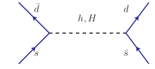
Figure 8: Tree-level diagram of scalar mediated $K-\overline{K}$ mixing.

Another set of constraints comes from the tree-level meson mixing processes mediated by $\{h,H\}$ as shown in Fig. 8. The major constraints arise from $K-\overline{K}$ and $B-\overline{B}$ mixing mass difference. The effective Hamiltonian leading to meson mixing may be written as

$$\mathcal{H}_{\text{eff}}=\sum_{k=h,H}\Bigg{(}\frac{C_{L_{k}}^{2}(\Lambda)}{2m_{k}^{2}}\mathcal{O}_{2}+\frac{C_{R_{k}}^{2}(\Lambda)}{2m_{k}^{2}}\widetilde{\mathcal{O}}_{2}+\frac{C_{L_{k}}(\Lambda)C_{R_{k}}(\Lambda)}{m_{k}^{2}}\mathcal{O}_{4}\Bigg{)},$$ (6.84)

with reference to the operators given in Sec. 4.4. Both the quantities in Table XVI are computed using magic numbers given in Appendix. C. The $\Delta M$’s obtained this way were constrained using the central value of the experimental results. In the case of $B-\overline{B}$, we also included an analysis with $\Delta M^{\text{SM+NP}}/\Delta M^{\text{SM}}$, since there is an attempt to reduce theoretical uncertainties of the SM prediction of $\Delta M_{B}$ DiLuzio:2019jyq . This gives a more stringent constraint quoted in parenthesis in Table XVI.

Process	Exp. Bound (GeV)	Constraint
$K-\overline{K}$	$(3.484\pm 0.006)\times 10^{-15}$	$|(V_{L_{f}}\mathcal{Y}_{F}\mathcal{Y}_{F}^{\dagger}V_{L_{f}}^{\dagger})_{ds}|\leq 1.06(\frac{M_{F}}{1\text{TeV}})^{2}$
$B-\overline{B}$	$(3.334\pm 0.013)\times 10^{-13}$	$|(V_{L_{f}}\mathcal{Y}_{F}\mathcal{Y}_{F}^{\dagger}V_{L_{f}}^{\dagger})_{db}|\leq 0.214(\frac{M_{F}}{1\text{TeV}})^{2}\left(4.21\times 10^{-2}(\frac{M_{F}}{1\text{TeV}})^{2}\right)$

Table XVI: Constraints from mass differences of neutral mesons. The results are quoted as a function of vector-like quark mass $M_{F}$(TeV). The NP contributions were constrained against the central value of experimental results. The constraint given in the parenthesis is obtained using $\Delta M^{\text{SM+NP}}/\Delta M^{\text{SM}}$.

7 Neutral Current B-anomalies

The experimental results on several $b\to s\mu^{+}\mu^{-}$ processes deviate significantly from the Standard Model predictions. Over the years the discrepancies have been observed in branching ratios of $B\to K^{(*)}\mu^{+}\mu^{-}$, $B_{s}\to\phi\mu^{+}\mu^{-}$, and $B_{s}\to\mu^{+}\mu^{-}$, and in the angular distribution of $B\to K^{*}\mu^{+}\mu^{-}$. In particular, there is a combined $3.1\leavevmode\nobreak\ \sigma$ discrepancy with the measurements of the lepton flavor universality (LFU) ratio $R_{K^{(*)}}=\Gamma(B\to K^{(*)}\mu^{+}\mu^{-})/\Gamma(B\to K^{(*)}e^{+}e^{-})$. The SM calculations of these observables are devoid of any hadronic uncertainties as they cancel out in the ratio leading to clean and highly accurate predictions Bordone:2016gaq :

$$R_{K}^{SM} =1.0004^{+0.0008}_{-0.0007},$$ (7.85)

$$R_{K^{*}}^{SM} =\begin{cases}0.906\pm 0.028\quad q^{2}\in[0.045,1.1]\leavevmode\nobreak\ \mathrm{GeV}^{2},\\ 1.00\pm 0.01\quad\quad q^{2}\in[1.1,6]\leavevmode\nobreak\ \mathrm{GeV}^{2},\end{cases}$$

where, $q$ denotes the dilepton mass. The most precise measurement of these ratios so far has been by the LHCb:

$$R_{K} =0.846^{+0.042+0.013}_{-0.039-0.012}\quad q^{2}\in[1.1,6]\leavevmode\nobreak\ \mbox{GeV}^{2},\leavevmode\nobreak\ \text{\cite[cite]{\@@bibref{Authors Phrase1YearPhrase2}{LHCb:2021trn}{\@@citephrase{(}}{\@@citephrase{)}}}}$$ (7.86)

$$R_{K^{*}} =\begin{cases}0.66^{+0.11}_{-0.07}\pm 0.024\quad q^{2}\in[0.045,1.1]\leavevmode\nobreak\ \mathrm{GeV}^{2},\\ 0.69^{+0.113}_{-0.069}\pm 0.047\quad q^{2}\in[1.1,6]\leavevmode\nobreak\ \mathrm{GeV}^{2}.\\ \end{cases}\leavevmode\nobreak\ \text{\cite[cite]{\@@bibref{Authors Phrase1YearPhrase2}{Aaij:2017vbb}{\@@citephrase{(}}{\@@citephrase{)}}}}$$

$R_{K^{*}}$ measurements have also been done by Belle Abdesselam:2019wac

$$R_{K^{*}} =\begin{cases}0.52^{+0.36}_{-0.26}\pm 0.05\quad q^{2}\in[0.045,1.1]\leavevmode\nobreak\ \mathrm{GeV}^{2},\\ 0.96^{+0.45}_{-0.29}\pm 0.11\quad q^{2}\in[1.1,6]\leavevmode\nobreak\ \mathrm{GeV}^{2},\\ 0.90^{+0.27}_{-0.21}\pm 0.10\quad q^{2}\in[0.1,8]\leavevmode\nobreak\ \mathrm{GeV}^{2},\\ 1.18^{+0.52}_{-0.32}\pm 0.10\quad q^{2}\in[15,19]\leavevmode\nobreak\ \mathrm{GeV}^{2},\\ 0.94^{+0.17}_{-0.14}\pm 0.08\quad q^{2}\in[0.045,]\leavevmode\nobreak\ \mathrm{GeV}^{2},\\ \end{cases}$$ (7.87)

but with considerably larger errors compared to LHCb. Another important discrepancy has been observed in the branching ratio of $B_{s}\to\mu^{+}\mu^{-}$ whose theoretical and experimental values are given in Table XVII. These deviations of experimental measurements from the SM predictions, referred to as the neutral current B-anomalies, could be clear signals of new physics. In this section, we explore the contribution to these processes from the LRSM with universal seesaw in the phenomenologically interesting parity symmetric version.

The contributions to neutral current B-anomalies in this model arise from the Lagrangian

$$\mathcal{L}_{Z_{i}}=\sum_{i=1}^{2}\frac{1}{2}M_{Z_{i}}^{2}(Z_{i_{\mu}})^{2}+\left(C_{L_{i}}^{bs}(\overline{b}_{L}\gamma^{\mu}s_{L})+C_{R_{i}}^{bs}(\overline{b}_{R}\gamma^{\mu}s_{R})+C_{L_{i}}^{\ell\ell}(\overline{\ell}_{L}\gamma^{\mu}\ell_{L})+C_{R_{i}}^{\ell\ell}(\overline{\ell}_{R}\gamma^{\mu}\ell_{R})\right)Z_{i_{\mu}},$$ (7.88)

where $\ell=\{e,\mu\}$. Integrating out $Z_{1,2}$ at tree-level gives the effective Lagrangian:

$$\mathcal{L}_{\text{eff}}= -\sum_{i=1}^{2}\frac{1}{M_{Z_{i}}^{2}}\Big{[}C_{L_{i}}^{bs}C_{L_{i}}^{\ell\ell}(\overline{b}_{L}\gamma^{\mu}s_{L})(\overline{\ell}_{L}\gamma_{\mu}\ell_{L})+C_{L_{i}}^{bs}C_{R_{i}}^{\ell\ell}(\overline{b}_{L}\gamma^{\mu}s_{L})(\overline{\ell}_{R}\gamma_{\mu}\ell_{R})$$ (7.89)

$$+C_{R_{i}}^{bs}C_{L_{i}}^{\ell\ell}(\overline{b}_{R}\gamma^{\mu}s_{R})(\overline{\ell}_{L}\gamma_{\mu}\ell_{L})+C_{R_{i}}^{bs}C_{R_{i}}^{\ell\ell}(\overline{b}_{R}\gamma^{\mu}s_{R})(\overline{\ell}_{R}\gamma_{\mu}\ell_{R})$$

$$+\frac{1}{2}(C^{bs}_{L_{i}})^{2}(\overline{b}_{L}\gamma_{\mu}s_{L})^{2}+\frac{1}{2}(C^{bs}_{R_{i}})^{2}(\overline{b}_{R}\gamma_{\mu}s_{R})^{2}+C^{bs}_{L_{i}}C^{bs}_{R_{i}}(\overline{b}_{L}\gamma_{\mu}s_{L})(\overline{b}_{R}\gamma^{\mu}s_{R})\Big{]}.$$

Compared to Eqns. (4.44),  (4.45) and Appendix. A, certain changes have been made to keep the notations simple. Firstly, the factor $g_{L}/\cos\theta_{W}$ has been absorbed into the coefficients $C_{{L,R}_{i}}$. Furthermore, $C^{bs}_{{L,R}_{i}}\equiv\widetilde{C}^{bs}_{{L,R}_{i}}$ while $C^{\ell\ell}_{{L,R}_{i}}\equiv\widetilde{C}^{\ell\ell}_{{L,R}_{i}}$ defined in Appendix. A. From the two expressions above, it is evident that the couplings relevant to resolving neutral current B-anomalies also contribute to $B_{s}-\overline{B}_{s}$ mixing as well as $Z_{i}$ decays. Therefore, the main constraints arise from

• The $B_{s}-\overline{B_{s}}$ mass difference: $\Delta M_{s}^{\text{NP+SM}}/\Delta M_{s}^{\text{SM}}$,

• Lepton flavour universality violation of $Z$ decays: $\Gamma(Z\to\mu^{+}\mu^{-})/\Gamma(Z\to e^{+}e^{-})$, and the individual branching ratios.

One would also need to consider the following observables in reconciling the B-anomalies:

• Muonic decay of $B_{s}$ meson: $\text{BR}(B_{s}\to\mu^{+}\mu^{-})^{\text{NP+SM}}/\text{BR}(B_{s}\to\mu^{+}\mu^{-})^{\text{SM}}$,

• Mixing induced $\mathcal{CP}$ asymmetry given by $A_{\mathcal{CP}}^{\text{mix}}(B_{s}\rightarrow J/\psi\phi)=\sin(\phi_{\Delta}-2\beta_{s})$ Lenz:2006hd with the value $-0.021\pm 0.031$  HFLAV:2019otj , where, $\phi_{\Delta}$ is defined as $\arg\Bigg{(}\dfrac{\Delta M_{s}^{\text{NP+SM}}}{\Delta M_{s}^{\text{SM}}}\Bigg{)}$ with $\beta_{s}=0.01843^{+0.00048}_{-0.00034}$ Charles:2004jd .

Observable	SM prediction	Experimental Value
$\frac{\displaystyle\Gamma(Z\to\mu^{+}\mu^{-})}{\displaystyle\Gamma(Z\to e^{+}e^{-})}$	$\simeq 1$	$1.0001\pm 0.0024$.
$\Delta M_{s}$	$(18.77\pm 0.86)\text{ps}^{-1}$	$(17.749\pm 0.020)\text{ps}^{-1}$
$BR(Z\to e^{+}e^{-})$	$(3.3663\pm 0.0012)\%$	$(3.3632\pm 0.0042)\%$
$BR(Z\to\mu^{+}\mu^{-})$	$(3.3663\pm 0.0012)\%$	$(3.3662\pm 0.0066)\%$
$BR(B_{s}\to\mu^{+}\mu^{-})$	$(3.65\pm 0.23)\times 10^{-9}$	$(3.09^{+0.46\leavevmode\nobreak\ +0.15}_{-0.43\leavevmode\nobreak\ -0.11})\times 10^{-9}$ LHCb:2021awg ; LHCb:2021vsc

Table XVII: Observables constraining the model parameters that contribute to resolving neutral current B-anomalies.

Assuming the couplings are real, the constraint from $B_{s}-\overline{B}_{s}$ mixing, allowing $2\,\sigma$ deviation, is

$$\frac{\Delta M_{s}^{\text{NP+SM}}}{\Delta M_{s}^{\text{SM}}}\leq\frac{\Delta M_{s}^{\text{exp}}}{\Delta M_{s}^{\text{SM}}}\equiv 0.95\pm 0.04\Rightarrow|R_{bs}|\leq 1.41\times 10^{-5}.$$ (7.90)

The LFU violation of Z decays can arise due to NP in either electron- or muon-sector, or both. For simplicity, we assume that the NP appears only in one of these sectors at a time leading to the following constraints, allowing $2\,\sigma$ deviation:

$$\frac{\Gamma(Z\to\mu^{+}\mu^{-})}{\Gamma(Z\to e^{+}e^{-})}\Rightarrow\begin{cases}|R_{\mu\mu}|\leq 1.74\times 10^{-3},\\ |R_{ee}|\leq 1.81\times 10^{-3}.\end{cases}$$ (7.91)

From these constraints, the largest allowed values of the conventional Wilson coefficients are tabulated in Table XVIII along with the respective LFU ratios. The NP WCs in terms of the model parameters are Altmannshofer:2021qrr

$$C_{9\,(10)}^{\ell} =\mp\frac{4\sqrt{2}\pi}{8G_{F}\alpha_{\text{em}}V_{tb}V_{ts^{*}}}\sum_{i=1}^{2}\left(\frac{1}{M_{Z_{i}}^{2}}C_{L_{i}}^{bs}\left(C_{L_{i}}^{\ell\ell}\pm C_{R_{i}}^{\ell\ell}\right)\right),$$ (7.92)

$$C_{9\,(10)}^{{}^{\prime}\ell} =\mp\frac{4\sqrt{2}\pi}{8G_{F}\alpha_{\text{em}}V_{tb}V_{ts^{*}}}\sum_{i=1}^{2}\left(\frac{1}{M_{Z_{i}}^{2}}C_{R_{i}}^{bs}\left(C_{L_{i}}^{\ell\ell}\pm C_{R_{i}}^{\ell\ell}\right)\right).$$

We see that the NP in electron-sector can improve the theoretical prediction of $R_{K^{(*)}}$ slightly due to the large right-handed current ($C_{9}^{{}^{\prime}e}=C_{10}^{{}^{\prime}e}$) (see also Refs. Geng:2017svp ; DAmico:2017mtc ; Datta:2019zca ) contribution in the denominator. This, however, is not sufficient to explain all the $b\to s\mu^{+}\mu^{-}$ related anomalies which points towards NP in the muonic sector. The NP in the muon-sector in this model worsens the $R_{K^{(*)}}$ prediction due to the large right-handed current $C_{9}^{{}^{\prime}\mu}=C_{10}^{{}^{\prime}\mu}$ appearing in the numerator, although it can explain the observed $\text{BR}(B_{s}\to\mu^{+}\mu^{-})$.

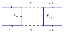
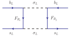
(a)                                             (b)

Figure 9: Box diagram contributing to $C_{9}$ from $\sigma_{L}$ mediator (a) and $B_{s}-\overline{B}_{s}$ mixing arising from the same mediator (b). $F$ represents VL-down type quark whereas $E$ represents VL-lepton.

Wilson coefficient	Value	Observable
$C_{9}^{e}=-C_{10}^{e}$	$-2.74\times 10^{-4}$	$R_{K}=0.95$
		$R_{K^{*}}=0.96$
$C_{9}^{{}^{\prime}e}=C_{10}^{{}^{\prime}e}$	$-9.03\times 10^{-1}$
		$\text{BR}(B_{s}\to\mu^{+}\mu^{-})=3.65\times 10^{-9}$
$C_{9}^{\mu}=-C_{10}^{\mu}$	$-2.63\times 10^{-4}$	$R_{K}=1.04$
		$R_{K^{*}}=1.03$
$C_{9}^{{}^{\prime}\mu}=C_{10}^{{}^{\prime}\mu}$	$-8.68\times 10^{-1}$
		$\text{BR}(B_{s}\to\mu^{+}\mu^{-})=2.35\times 10^{-9}$

Table XVIII: Maximum values of NP Wilson coefficients (Eq. (7.92)) allowed by the model parameters consistent with $B_{s}-\overline{B}_{s}$ mixing (Eq. (7.90)) and LFUV of $Z$ decays (Eq. (7.91)) and the corresponding extremum values of the observable. Note that NP from only one of the electron or muon sectors is turned on at a time.

Since the global fit to the neutral current B-anomalies alludes to a muon-specific left-handed current Altmannshofer:2021qrr , box diagram contribution mediated by left-handed scalar field $\sigma_{L}$ (assuming no mixing with $\sigma_{R}$ such that $(m_{\sigma_{L}}=m_{h})\ll(m_{\sigma_{R}}=m_{H})$), as shown in Fig. 9 (a), leading to $C_{9}^{\mu}=-C_{10}^{\mu}$ was also explored. The NP WC from the box diagram is

$$C_{9}^{\mu}=-C_{10}^{\mu}=-\frac{\sqrt{2}}{128\pi G_{F}\alpha_{\text{em}}}\frac{1}{V_{tb}V_{ts}^{*}}\frac{|y_{\mu}|^{2}y_{s}y^{*}_{b}}{4m_{\sigma_{L}}^{2}}\mathcal{F}(x_{i},x_{j}),$$ (7.93)

where,

$$\mathcal{F}(x_{i},x_{j})=\frac{x_{i}^{2}\ln{x_{i}}}{(x_{i}-1)^{2}(x_{i}-x_{j})}-\frac{x_{j}^{2}\ln{x_{j}}}{(x_{j}-1)^{2}(x_{i}-x_{j})}+\frac{1}{(x_{j}-1)(x_{i}-1)},$$ (7.94)

with $x_{i}=\dfrac{m_{F_{i}}}{m_{\sigma_{L}}}$ and $x_{j}=\dfrac{m_{E_{j}}}{m_{\sigma_{L}}}$. Here, $y_{\mu}$, $y_{s}$ and $y_{b}$ are Yukawa couplings of $\mu_{L}$, $s_{L}$ and $b_{L}$, respectively, to $\sigma_{L}$. The coupling of quarks $b$ and $s$ to $\sigma_{L}$ and down-type VLFs lead to $B_{s}-\overline{B}_{s}$ mixing as shown in Fig. 9 (b). The mass difference (procedure for the calculation is described in Sec. 4.4 and the magic numbers are given in Appendix. B.3) is given by

$$\Delta M_{s}=\frac{0.86}{32\pi^{2}}\frac{|y_{b}|^{2}|y_{s}|^{2}}{4m_{\sigma_{L}}^{2}}\frac{8}{3}f^{2}_{B_{s}}M_{B_{s}}B_{1}(\mu_{b})\mathcal{F}(x_{i},x_{j}),$$ (7.95)

with $x_{i}=\dfrac{m_{F_{i}}}{m_{\sigma_{L}}}$ and $x_{j}=\dfrac{m_{F_{j}}}{m_{\sigma_{L}}}$. The constraint arising from $\Delta M_{s}$ is extremely severe to allow large values of WCs required to explain the observed $R_{K^{(*)}}$. We conclude that this model, although it has room to improve the $R_{K^{(*)}}$ prediction, cannot completely resolve the $b\to s\mu^{+}\mu^{-}$ anomaly.

8 Anomalous Magnetic Moment of Muon

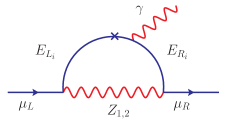
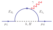
(a)                                            (b)

Figure 10: Diagrams leading to correction to AMM.

The anomalous magnetic moment of muon $a_{\mu}=(g_{\mu}-2)/2$ is predicted to be $a_{\mu}^{\textnormal{SM}}=116591810(43)\times 10^{-11}$ Davier:2019can ; Aoyama:2020ynm ; Davier:2010nc ; Gerardin:2020gpp . The measurements of $a_{\mu}$ at Fermilab National Accelerator Laboratory (FNAL), $a_{\mu}(\textnormal{FNAL})=116592040(54)\times 10^{-11}$  Muong-2:2021ojo , which agrees with the previous Brookhaven National Laboratory (BNL) E821 measurement Muong-2:2006rrc ; Muong-2:2001kxu is at odds with the SM prediction. The difference, $\Delta a_{\mu}=a_{\mu}^{\text{exp}}-a_{\mu}^{\text{th}}\simeq(251\pm 59)\times 10^{-11}$, is a $4.2\,\sigma$ discrepancy. (There is an ambiguity that emerged recently with the results from the BMW collaboration Borsanyi:2020mff which agrees with the experimental measurement within $1.6\leavevmode\nobreak\ \sigma$.) The discrepancy is another major hint towards BSM physics. The neutral scalars $h$ and $H$, and the neutral gauge bosons $Z_{1}$ and $Z_{2}$ in the LRSM with universal seesaw can mediate significant chirally enhanced one-loop corrections to $a_{\mu}$, as shown in Fig. 10, potentially resolving the anomaly in AMM of muon.

The corrections to AMM arise from the following Lagrangian:

$$\mathcal{L} \supset g_{L}\cos\theta_{W}\overline{\mu}\gamma^{\mu}Z_{1_{\mu}}\left[\left\{\frac{\sin\xi}{2\sqrt{\cos 2\theta_{W}}}\frac{g_{Y}^{2}}{g_{L}^{2}}-\cos\xi\left(\frac{1}{2}+\frac{1}{2}\frac{g_{Y}^{2}}{g_{L}^{2}}\right)\right\}V_{L}\rho_{L}^{\dagger}\,\text{P}_{\text{L}}+\frac{\kappa_{R}\sin\xi}{2\kappa_{L}\sqrt{\cos 2\theta_{W}}}V_{L}\rho_{L}^{\dagger}\,\text{P}_{\text{R}}\right]F$$

$$-g_{L}\cos\theta_{W}\overline{\mu}\gamma^{\mu}Z_{2_{\mu}}\left[\left\{\frac{\cos\xi}{2\sqrt{\cos 2\theta_{W}}}\frac{g_{Y}^{2}}{g_{L}^{2}}+\sin\xi\left(\frac{1}{2}+\frac{1}{2}\frac{g_{Y}^{2}}{g_{L}^{2}}\right)\right\}V_{L}\rho_{L}^{\dagger}\text{P}_{\text{L}}-\frac{\kappa_{R}\cos\xi}{2\kappa_{L}\sqrt{\cos 2\theta_{W}}}V_{L}\rho_{L}^{\dagger}\text{P}_{\text{R}}\right]F$$

$$+\overline{\mu}\,h\left[\frac{\cos\zeta}{\sqrt{2}}\left(\left\{V_{L}\mathcal{Y}-\frac{1}{2}(V_{L}\mathcal{Y}\,\rho_{L}\rho_{L}^{\dagger}\frac{\kappa_{R}^{2}}{\kappa_{L}^{2}}+V_{L}\rho_{L}^{\dagger}\rho_{L}\mathcal{Y})\right\}\text{P}_{\text{R}}-\left\{V_{L}\rho^{\dagger}_{L}\mathcal{Y}^{\dagger}\rho_{L}^{\dagger}\frac{\kappa_{R}}{\kappa_{L}}\right\}\text{P}_{\text{L}}\right)\right.$$

$$\left.-\frac{\sin\zeta}{\sqrt{2}}\left(\left\{V_{L}\mathcal{Y}-\frac{1}{2}(V_{L}\mathcal{Y}\,\rho_{L}\rho_{L}^{\dagger}+V_{L}\frac{\kappa_{R}^{2}}{\kappa_{L}^{2}}\rho_{L}^{\dagger}\rho_{L}\mathcal{Y})\right\}\text{P}_{\text{L}}-\left\{V_{L}\rho^{\dagger}_{L}\mathcal{Y}^{\dagger}\rho_{L}^{\dagger}\frac{\kappa_{R}}{\kappa_{L}}\right\}\text{P}_{\text{R}}\right)\right]F$$

$$+\overline{\mu}\,H\left[\frac{\sin\zeta}{\sqrt{2}}\left(\left\{V_{L}\mathcal{Y}-\frac{1}{2}(V_{L}\mathcal{Y}\,\rho_{L}\rho_{L}^{\dagger}\frac{\kappa_{R}^{2}}{\kappa_{L}^{2}}+V_{L}\rho_{L}^{\dagger}\rho_{L}\mathcal{Y})\right\}\text{P}_{\text{R}}-\left\{V_{L}\rho^{\dagger}_{L}\mathcal{Y}^{\dagger}\rho_{L}^{\dagger}\frac{\kappa_{R}}{\kappa_{L}}\right\}\text{P}_{\text{L}}\right)\right.$$

$$\left.+\frac{\cos\zeta}{\sqrt{2}}\left(\left\{V_{L}\mathcal{Y}-\frac{1}{2}(V_{L}\mathcal{Y}\,\rho_{L}\rho_{L}^{\dagger}+V_{L}\frac{\kappa_{R}^{2}}{\kappa_{L}^{2}}\rho_{L}^{\dagger}\rho_{L}\mathcal{Y})\right\}\text{P}_{\text{L}}-\left\{V_{L}\rho^{\dagger}_{L}\mathcal{Y}^{\dagger}\rho_{L}^{\dagger}\frac{\kappa_{R}}{\kappa_{L}}\right\}\text{P}_{\text{R}}\right)\right]F,$$ (8.96)

where, $\text{P}_{\text{\{L,R\}}}$ are left- and right-handed projection operators, and $F$ represents the heavy VL-leptons. Compared to the general form of the interaction Lagrangian

$$\mathcal{L}\supset\sum_{F,X}\overline{\mu}\left[C_{V}\gamma^{\mu}+C_{A}\gamma^{\mu}\gamma^{5}\right]F\,X_{\mu}+\sum_{F,H}\overline{\mu}\left[C_{S}+C_{P}\gamma^{5}\right]F\,H\,,$$ (8.97)

The corrections to AMM Leveille:1977rc , under the assumption $m_{\mu}\to 0$, arising from the VL-lepton mass enhancements are:

$$\left[a_{\mu}\right]_{X}= \frac{m_{\mu}m_{F}}{4\pi^{2}}(C_{A}^{2}-C_{V}^{2})\mathcal{F}(m_{F},m_{X})$$ (8.98)

$$\left[a_{\mu}\right]_{H}= \frac{m_{\mu}m_{F}}{8\pi^{2}}(C_{S}^{2}-C_{P}^{2})\mathcal{G}(m_{F},m_{H})$$

with

$$\mathcal{F}(m_{F},m_{X})= \frac{\left[m_{F}^{6}-4m_{X}^{6}+3m_{X}^{4}m_{F}^{2}+6m_{X}^{4}m_{F}^{2}\ln{\dfrac{m_{X}^{2}}{m_{F}^{2}}}\right]}{4m_{X}^{2}(m_{X}^{2}-m_{F}^{2})^{3}}$$ (8.99)

$$\mathcal{G}(m_{F},m_{X})= \frac{\left[m_{F}^{4}+3m_{H}^{4}-4m_{H}^{2}m_{F}^{2}+2m_{H}^{4}\ln{\dfrac{m_{F}^{2}}{m_{H}^{2}}}\right]}{2(m_{F}^{2}-m_{H}^{2})^{3}}$$

A single-family mixing between muon and the corresponding VLF is not enough to resolve the anomaly in AMM due to the constraint from muon mass. To avoid this, we consider a case where muon mixes with two VL-leptons in a basis where the muon mass is negligible:

$$\left(\overline{\mu}_{L}\leavevmode\nobreak\ \overline{E}_{e_{L}}\leavevmode\nobreak\ \overline{E}_{\mu_{L}}\right)\begin{pmatrix}0&&0&&y_{\mu}\kappa_{L}\\ 0&&0&&M_{1}\\ y_{\mu}\kappa_{R}&&M_{1}&&M_{2}\end{pmatrix}\begin{pmatrix}\mu_{R}\\ E_{e_{R}}\\ E_{\mu_{R}}\end{pmatrix},$$ (8.100)

such that $y_{\mu}\kappa_{L}\ll\{M_{1},\,M_{2}\}$. The mixing matrix $\mathcal{M}_{\mu}$ is diagonalized by a bi-unitary transform of the form

$$\text{Diag}(0,\,M_{E},\,M_{M})=U_{L}\mathcal{M}_{\mu}U_{R}^{\dagger}$$ (8.101)

where,

$$U_{X=\{L,\,R\}}=\begin{pmatrix}c_{X_{1}}&s_{X_{1}}&0\\ -c_{X_{2}}s_{X_{1}}&c_{X_{1}}c_{X_{2}}&s_{X_{2}}\\ -s_{X_{1}}s_{X_{2}}&-c_{X_{1}}s_{X_{2}}&c_{X_{2}}\end{pmatrix}.$$ (8.102)

Here, $c\,(s)$ stand for $\cos\,(\sin)$. The mixing angles and the mass eigenstates are

$$L_{1}=\arctan(\frac{-y_{\mu}\kappa_{L}}{M_{1}}), L_{2}=\frac{1}{2}\arctan\left(-\frac{2M_{2}\sqrt{M_{1}^{2}+y_{\mu}^{2}\kappa_{L}^{2}}}{M_{2}^{2}+(\kappa_{R}^{2}-\kappa_{L}^{2})y_{\mu}^{2}}\right)$$ (8.103)

$$R_{1}=\arctan(\frac{-y_{\mu}\kappa_{R}}{M_{1}}), R_{2}=\frac{1}{2}\arctan\left(-\frac{2M_{2}\sqrt{M_{1}^{2}+y_{\mu}^{2}\kappa_{R}^{2}}}{M_{2}^{2}-(\kappa_{R}^{2}-\kappa_{L}^{2})y_{\mu}^{2}}\right)$$

$$M_{E,\,M}=\frac{1}{2}\left(2M_{1}^{2}+M_{2}^{2}+(\kappa_{L}^{2}+\kappa_{R}^{2})y_{\mu}^{2}\mp\sqrt{4M_{2}^{2}(M_{1}^{2}+\kappa_{L}^{2}y_{\mu}^{2})+\left(M_{2}^{2}+(\kappa_{R}^{2}-\kappa_{L}^{2})y_{\mu}^{2}\right)^{2}}\right)$$ (8.104)

The mixing between $Z_{L}-Z_{R}$ can be ignored such that $Z_{1\,(2)}\equiv Z_{L\,(R)}$, whereas $\sigma_{L}-\sigma_{R}$ mixing as of Eq. (2.6) is required to obtain a chiral enhancement. The total correction to AMM is

$$a_{\mu}= -\frac{m_{\mu}}{4\pi^{2}}\Bigg{[}\frac{g_{L}^{4}\tan^{2}\theta_{W}}{4(g_{L}^{2}-g_{Y}^{2})}c_{L_{1}}c_{R_{1}}s_{L_{1}}s_{R_{1}}\left\{c_{L_{2}}c_{R_{2}}M_{E}\mathcal{F}(M_{E},m_{Z_{R}})+s_{L_{2}}s_{R_{2}}M_{M}\mathcal{F}(M_{M},m_{Z_{R}})\right\}$$ (8.105)

$$\qquad\leavevmode\nobreak\ \leavevmode\nobreak\ \leavevmode\nobreak\ \leavevmode\nobreak\ \frac{y_{\mu}^{2}\sin 2\zeta}{8}c_{L_{1}}c_{R_{1}}\left\{s_{L_{2}}s_{R_{2}}M_{E}\mathcal{G}(M_{E},m_{h})+c_{L_{2}}c_{R_{2}}M_{E}\mathcal{G}(M_{M},m_{h})\right.$$

$$\left.\qquad\qquad\qquad\qquad\leavevmode\nobreak\ \leavevmode\nobreak\ \leavevmode\nobreak\ \leavevmode\nobreak\ \leavevmode\nobreak\ \leavevmode\nobreak\ -s_{L_{2}}s_{R_{2}}M_{E}\mathcal{G}(M_{E},m_{H})-c_{L_{2}}c_{R_{2}}M_{E}\mathcal{G}(M_{M},m_{H})\right\}\Bigg{]}$$

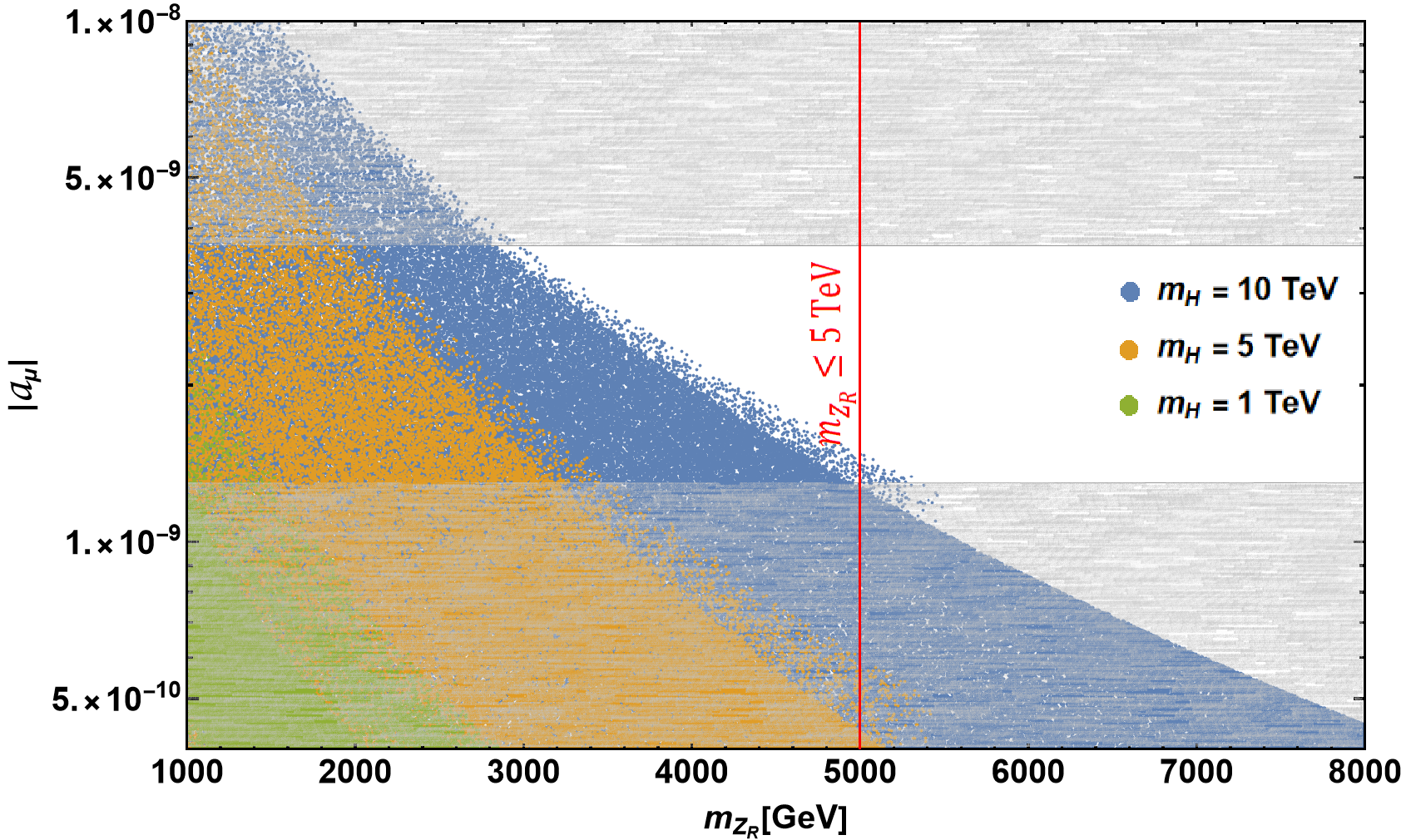
Figure 11: Scatter plot of correction to AMM as a function for $Z_{R}$ mass for different values of the heavy higgs mass. The Yukawa coupling $y_{\mu}=1$ and bare masses $M_{1,2}$ was varied between 0.5 TeV and 10 TeV. The shaded regions lie outside the required $2\,\sigma$ range of $a_{\mu}$. The region to the left of the vertical red line is excluded by the lower bound on $Z_{R}$ mass ATLAS:2019erb .

The scatter plot in Fig. 11 shows that the correction to AMM is not large enough to explain the $4.2\,\sigma$ discrepancy for scalar masses in the experimentally accessible ($\leq\mathcal{O}$ (TeV)) range.

9 Conclusion

This paper presents a comprehensive description of the left-right symmetric model with a universal seesaw mechanism for generating fermion masses. The direct coupling of SM fermions with their VLF singlet partners leads to tree-level flavor-changing neutral current interactions and has room for flavor and flavor-universality violating processes, making this a compelling model to explore various flavor anomalies that have come up in recent years. Full tree-level Lagrangian in the physical basis has been explored, allowing us to obtain constraints on the theory parameters from neutral and charged current mediated processes. The parity symmetric version, motivated by the axionless solution to the strong $\mathcal{CP}$ problem, was explored in great detail. The model was applied to find a solution to the neutral current B-anomalies and the AMM of muon. The constraints on the contributions from the model were found to be severe, ruling out the possibility of resolving the two anomalies. The contribution to $R_{K^{(*)}}$ is restricted by the stringent constraint appearing from the mass difference in $B_{s}-\overline{B}_{s}$ mixing. Although the model allows VLF mass-enhanced corrections to the AMM of muon, the constraint from muon mass eliminates any substantial correction to survive. We also found that the discrepancies observed in various LFU-violating processes mediated by charged current interactions could also not be simultaneously explained by the parameter space of the model.

Appendix A Neutral Current Interaction

The coefficients of neutral current interaction of $Z_{1}$ with SM fermions as defined in Eq. (4.44) are

$$C_{L_{1}} =\cos^{2}\theta_{W}\left[\cos\xi\left(T_{3L}-\frac{g_{Y}^{2}}{g_{L}^{2}}\frac{Y_{f_{L}}}{2}\right)-\frac{\sin\xi}{\sqrt{\cos 2\theta_{W}}}\left(-\frac{g_{Y}^{2}}{g_{L}^{2}}\frac{Y_{f_{L}}}{2}\right)\right],$$ (A.106)

$$\widetilde{C}_{L_{1}} =-\cos^{2}\theta_{W}\left[\cos\xi\left(T_{3L}-\frac{g_{Y}^{2}}{g_{L}^{2}}\frac{Y_{f_{L}}-Y_{F}}{2}\right)+\frac{\sin\xi}{\sqrt{\cos 2\theta_{W}}}\left(\frac{g_{Y}^{2}}{g_{L}^{2}}\frac{Y_{f_{L}}-Y_{F}}{2}\right)\right]\times R_{ij},$$

$$C_{R_{1}} =\cos^{2}\theta_{W}\left[\cos\xi\left(-\frac{g_{Y}^{2}}{g_{L}^{2}}\frac{Y_{f_{R}}}{2}\right)-\frac{\sin\xi}{\sqrt{\cos 2\theta_{W}}}\left(T_{3R}-\frac{g_{Y}^{2}}{g_{L}^{2}}\frac{Y_{f_{R}}}{2}\right)\right],$$

$$\widetilde{C}_{R_{1}} =\cos^{2}\theta_{W}\frac{\sin\xi}{\sqrt{\cos 2\theta_{W}}}\left(T_{3R}\right)\times\frac{\kappa_{R}^{2}}{\kappa_{L}^{2}}R_{ij},$$

whereas those of $Z_{2}$ with SM fermions as in Eq. (4.45) are as follows:

$$C_{L_{2}} =\cos^{2}\theta_{W}\left[\frac{\cos\xi}{\sqrt{\cos 2\theta_{W}}}\left(-\frac{g_{Y}^{2}}{g_{L}^{2}}\frac{Y_{f_{L}}}{2}\right)+\sin\xi\left(T_{3L}-\frac{g_{Y}^{2}}{g_{L}^{2}}\frac{Y_{f_{L}}}{2}\right)\right],$$ (A.107)

$$\widetilde{C}_{L_{2}} =\cos^{2}\theta_{W}\left[\frac{\cos\xi}{\sqrt{\cos 2\theta_{W}}}\left(\frac{g_{Y}^{2}}{g_{L}^{2}}\frac{Y_{f_{L}}-Y_{F}}{2}\right)-\sin\xi\left(T_{3L}-\frac{g_{Y}^{2}}{g_{L}^{2}}\frac{Y_{f_{L}}-Y_{F}}{2}\right)\right]\times R_{ij},$$

$$C_{R_{2}} =\cos^{2}\theta_{W}\left[\frac{\cos\xi}{\sqrt{\cos 2\theta_{W}}}\left(T_{3R}-\frac{g_{Y}^{2}}{g_{L}^{2}}\frac{Y_{f_{R}}}{2}\right)+\sin\xi\left(-\frac{g_{Y}^{2}}{g_{L}^{2}}\frac{Y_{f_{R}}}{2}\right)\right],$$

$$\widetilde{C}_{R_{2}} =-\cos^{2}\theta_{W}\frac{\cos\xi}{\sqrt{\cos 2\theta_{W}}}\left(T_{3R}\right)\times\frac{\kappa_{R}^{2}}{\kappa_{L}^{2}}R_{ij}.$$

Appendix B Input Parameters for Meson Mixing

Here, we provide various input parameters useful in computing the meson mixing mass difference. The strong coupling strengths at high scales Bethke:2009jm , $\alpha_{s}(\Lambda)$, are given in Table XIX.

Scale	$M_{Z_{1}}$	$M_{Z_{2}}$	$M_{W_{L}}$	$M_{W_{R}}$	$M_{h}$	$M_{H}$	$M_{t}$
$\Lambda$	91.187 GeV	5 TeV	80.379 GeV	4.219 TeV	125.10 GeV	10 TeV	172.9 GeV
$\bm{\alpha_{s}}$	0.1183	0.0824	0.1206	0.0837	0.1129	0.0774	0.1079

Table XIX: Values of the strong coupling constant at different energy scales.

B.1 $K-\overline{K}$ Mixing

Constants	$\mu$	$f_{K}$	$M_{K}$	$m_{s}$	$m_{d}$
Values	$2\text{ GeV}$	$159.8\text{ MeV}$	$467.611\text{ MeV}$	$93\text{ MeV}$	$4.67\text{ MeV}$
Constants	$R_{1}$	$R_{2}$	$R_{3}$	$R_{4}$	$R_{5}$
Values	1	-12.9	3.98	20.8	5.2

Table XX: Values of input parameters used in $K-\overline{K}$ mixing.

The meson mixing mass difference is given by $\Delta M_{K}=2\text{Re}\bra{K}\mathcal{H}\ket{\overline{K}}$. The matrix element at low energy scale is obtained as:

$$\bra{\overline{K}}\mathcal{H}_{\text{eff}}\ket{K}_{i}=\sum_{j=1}^{5}\sum_{r=1}^{5}(b_{j}^{(r,i)}+\eta c_{j}^{(r,i)})\eta^{a_{j}}C_{i}(\Lambda))R_{r}\bra{\overline{K}}\mathcal{Q}_{1}\ket{K},$$ (B.108)

with, $\langle\mathcal{O}_{1}\rangle=\frac{1}{3}M_{K}f^{2}_{K}B_{1}(\mu)$. The non-vanishing entries of the magic numbers are Ciuchini:1998ix :

$$a_{i}=(0.29,-0.69,0.79,-1.1,0.14)$$

$$b_{i}^{(11)} =(0.82,0,0,0,0),$$

$$b_{i}^{(22)} =(0,2.4,0.011,0,0),$$

$$b_{i}^{(23)} =(0,-0.63,0.17,0,0),$$

$$b_{i}^{(32)} =(0,-0.019,0.028,0,0),$$

$$b_{i}^{(33)} =(0,0.0049,0.43,0,0),$$

$$b_{i}^{(44)} =(0,0,0,4.4,0),$$

$$b_{i}^{(45)} =(0,0,0,1.5,-0.17),$$

$$b_{i}^{(54)} =(0,0,0,0.18,0),$$

$$b_{i}^{(55)} =(0,0,0,0.061,0.82),$$

$$c_{i}^{(11)} =(-0.016,0,0,0,0),$$ (B.109)

$$c_{i}^{(22)} =(0,-0.23,-0.002,0,0),$$

$$c_{i}^{(23)} =(0,-0.018,0.0049,0,0),$$

$$c_{i}^{(32)} =(0,0.0028,-0.0093,0,0),$$

$$c_{i}^{(33)} =(0,0.00021,0.023,0,0),$$

$$c_{i}^{(44)} =(0,0,0,-0.68,0.0055),$$

$$c_{i}^{(45)} =(0,0,0,-0.35,-0.0062),$$

$$c_{i}^{(54)} =(0,0,0,-0.026,-0.016),$$

$$c_{i}^{(55)} =(0,0,0,-0.013,0.018).$$

The coefficients and input parameters relevant to this calculation are given in Table XX.

B.2 $D-\overline{D}$ Mixing

Constants	$\mu$	$f_{D}$	$M_{D}$	$m_{u}$	$m_{c}$
Values	$2.8\text{ GeV}$	$201\text{ MeV}$	$1.864\text{ GeV}$	$2.01\text{ MeV}$	$1.01\text{ GeV}$
Constants	$B_{1}$	$B_{2}$	$B_{3}$	$B_{4}$	$B_{5}$
Values	0.865	0.82	1.07	1.08	1.455

Table XXI: Values of input parameters used in $D-\overline{D}$ mixing.

The mass difference is given by $\Delta M_{D}=2|\bra{D}\mathcal{H}\ket{\overline{D}}|$ with the renormalised operators being:

$$\langle\mathcal{O}_{1}\rangle =\frac{1}{3}M_{D}f^{2}_{D}B_{1}(\mu),$$ (B.110)

$$\langle\mathcal{O}_{2}\rangle =-\frac{5}{24}\left(\frac{M_{D}}{m_{u}(\mu)+m_{c}(\mu)}\right)^{2}M_{D}f^{2}_{D}B_{2}(\mu),$$

$$\langle\mathcal{O}_{3}\rangle =\frac{1}{24}\left(\frac{M_{D}}{m_{u}(\mu)+m_{c}(\mu)}\right)^{2}M_{D}f^{2}_{D}B_{3}(\mu),$$

$$\langle\mathcal{O}_{4}\rangle =\frac{1}{4}\left(\frac{M_{D}}{m_{u}(\mu)+m_{c}(\mu)}\right)^{2}M_{D}f^{2}_{D}B_{4}(\mu),$$

$$\langle\mathcal{O}_{5}\rangle =\frac{1}{12}\left(\frac{M_{D}}{m_{u}(\mu)+m_{c}(\mu)}\right)^{2}M_{D}f^{2}_{D}B_{5}(\mu).$$

The coefficients and input parameter values are listed in Table XXI and the non-vanishing entries of the magic numbers are Bona:2007vz :

$$a_{i}=(0.286,-0.692,0.787,-1.143,0.143)$$

$$b_{i}^{(11)} =(0.837,0,0,0,0),$$

$$b_{i}^{(22)} =(0,2.163,0.012,0,0),$$

$$b_{i}^{(23)} =(0,-0.567,0.176,0,0),$$

$$b_{i}^{(32)} =(0,-0.032,0.031,0,0),$$

$$b_{i}^{(33)} =(0,0.008,0.474,0,0),$$

$$b_{i}^{(44)} =(0,0,0,3.63,0),$$

$$b_{i}^{(45)} =(0,0,0,1.21,-0.19),$$

$$b_{i}^{(54)} =(0,0,0,0.14,0),$$

$$b_{i}^{(55)} =(0,0,0,0.045,0.839),$$

$$c_{i}^{(11)} =(-0.016,0,0,0,0),$$ (B.111)

$$c_{i}^{(22)} =(0,-0.20,-0.002,0,0),$$

$$c_{i}^{(23)} =(0,-0.016,0.006,0,0),$$

$$c_{i}^{(32)} =(0,-0.004,-0.010,0,0),$$

$$c_{i}^{(33)} =(0,0,0.025,0,0),$$

$$c_{i}^{(44)} =(0,0,0,-0.56,0.006),$$

$$c_{i}^{(45)} =(0,0,0,-0.29,-0.006),$$

$$c_{i}^{(54)} =(0,0,0,-0.019,-0.016),$$

$$c_{i}^{(55)} =(0,0,0,-0.009,0.018).$$

B.3 $B_{q}-\overline{B}_{q}$ Mixing

The operators used in evaluating $\Delta M_{B_{q}}=2|\bra{B_{q}}\mathcal{H}\ket{\overline{B}_{q}}|$ (in Sec. 4.4) are

$$\langle\mathcal{O}_{1}\rangle =f^{2}_{B_{q}}M_{B_{q}}\frac{8}{3}B_{1}(\mu_{b}),$$ (B.112)

$$\langle\mathcal{O}_{2}\rangle =f_{B_{q}}^{2}M_{B_{q}}\frac{-5M_{B_{q}}^{2}}{3(\overline{m}_{b}(\mu_{b})+\overline{m}_{q}(\mu_{b}))^{2}}B_{2}(\mu_{b}),$$

$$\langle\mathcal{O}_{3}\rangle =f_{B_{q}}^{2}M_{B_{q}}\frac{M_{B_{q}}^{2}}{3(\overline{m}_{b}(\mu_{b})+\overline{m}_{q}(\mu_{b}))^{2}}B_{3}(\mu_{b}),$$

$$\langle\mathcal{O}_{4}\rangle =f_{B_{q}}^{2}M_{B_{q}}\left[\frac{2M_{B_{q}}^{2}}{(\overline{m}_{b}(\mu_{b})+\overline{m}_{q}(\mu_{b}))^{2}}+\frac{1}{3}\right]B_{4}(\mu_{b}),$$

$$\langle\mathcal{O}_{5}\rangle =f_{B_{q}}^{2}M_{B_{q}}\left[\frac{2M_{B_{q}}^{2}}{3(\overline{m}_{b}(\mu_{b})+\overline{m}_{q}(\mu_{b}))^{2}}+1\right]B_{5}(\mu_{b}).$$

The central values of the combination of $f_{B}^{2}B_{i}(\mu_{b}=4.18\text{ GeV})$ used are as follows DiLuzio:2019jyq :

$$f_{B_{s}}^{2}B_{1}^{s}(\mu_{b}) = 0.0452\text{ GeV}^{2},$$

$$f_{B_{s}}^{2}B_{2}^{d}(\mu_{b}) = 0.0441\text{ GeV}^{2},$$

$$f_{B_{s}}^{2}B_{3}^{d}(\mu_{b}) = 0.0454\text{ GeV}^{2},$$

$$f_{B_{s}}^{2}B_{4}^{s}(\mu_{b}) = 0.0544\text{ GeV}^{2},$$

$$f_{B_{s}}^{2}B_{5}^{s}(\mu_{b}) = 0.0507\text{ GeV}^{2},$$

$$f_{B_{d}}^{2}B_{1}^{d}(\mu_{b}) = 0.0305\text{ GeV}^{2},$$ (B.113)

$$f_{B_{d}}^{2}B_{2}^{d}(\mu_{b}) = 0.0288\text{ GeV}^{2},$$

$$f_{B_{d}}^{2}B_{3}^{d}(\mu_{b}) = 0.0281\text{ GeV}^{2},$$

$$f_{B_{d}}^{2}B_{4}^{d}(\mu_{b}) = 0.0387\text{ GeV}^{2},$$

$$f_{B_{d}}^{2}B_{5}^{d}(\mu_{b}) = 0.0361\text{ GeV}^{2}.$$

The masses of quarks at $\mu_{b}$ are $m_{s}=77.9\text{ MeV}$, $m_{d}=3.94\text{ MeV}$ and $m_{b}=4.18\text{ GeV}$.

In Sec. 6, $B_{d}-\overline{B_{d}}$ mass difference was calculated using magic numbers. The renormalized operators in terms of $B_{i}(\mu)$ parameters are same as in Eq. (B.110) with {$M_{D}\to M_{B_{d}}$, $f_{D}\to f_{B_{d}}$, $m_{u}\to m_{b}$, $m_{c}\to m_{d}$}. Other relevant input parameters are given in Table XXII and the non-vanishing entries of the magic numbers are Becirevic:2001jj :

$$a_{i}=(0.286,-0.692,0.787,-1.143,0.143)$$ (B.114)

$$b_{i}^{(11)} =(0.865,0,0,0,0),$$

$$b_{i}^{(22)} =(0,1.879,0.012,0,0),$$

$$b_{i}^{(23)} =(0,-0.493,0.18,0,0),$$

$$b_{i}^{(32)} =(0,-0.044,0.035,0,0),$$

$$b_{i}^{(33)} =(0,0.011,0.54,0,0),$$

$$b_{i}^{(44)} =(0,0,0,2.87,0),$$

$$b_{i}^{(45)} =(0,0,0,0.961,-0.22),$$

$$b_{i}^{(54)} =(0,0,0,0.09,0),$$

$$b_{i}^{(55)} =(0,0,0,0.029,0.863),$$

$$c_{i}^{(11)} =(-0.017,0,0,0,0),$$ (B.115)

$$c_{i}^{(22)} =(0,-0.18,-0.003,0,0),$$

$$c_{i}^{(23)} =(0,-0.014,0.008,0,0),$$

$$c_{i}^{(32)} =(0,-0.005,-0.012,0,0),$$

$$c_{i}^{(33)} =(0,0,0.028,0,0),$$

$$c_{i}^{(44)} =(0,0,0,-0.48,0.005),$$

$$c_{i}^{(45)} =(0,0,0,-0.25,-0.006),$$

$$c_{i}^{(54)} =(0,0,0,-0.013,-0.016),$$

$$c_{i}^{(55)} =(0,0,0,-0.007,0.019),$$

Constants	$\mu$	$f_{B_{d}}$	$M_{B_{d}}$	$m_{b}$	$m_{d}$
Values	$4.6\text{ GeV}$	$200\text{ MeV}$	$5.279\text{ GeV}$	$4.61\text{ GeV}$	$5.4\text{ MeV}$
Constants	$B_{1}$	$B_{2}$	$B_{3}$	$B_{4}$	$B_{5}$
Values	0.87	0.82	1.02	1.16	1.91

Table XXII: Values of input parameters used in $B_{d}-\overline{B}_{d}$ mixing.

Appendix C Form Factors for Meson Decay

The form factor that appears in Eq. (4.66) describing the decay width of meson to lighter meson and charged leptons takes the form Melikhov:2000yu

$$f_{+}(q^{2})=f_{+}(0)/(1-\frac{q^{2}}{M_{V}^{2}}).$$ (C.116)

The values of the form factors and the vector meson masses are given in Table XXIII.

Transition	$f_{+}(0)$	$M_{V}$(GeV)
$K\to\pi$	0.9709 Carrasco:2016kpy	0.892
$B\to\pi$	0.29	5.32
$B\to K$	0.36	5.42
$D\to\pi$	0.69	2.01
$D_{s}\to K$	0.72	2.01

Table XXIII: Parameter values used in calculation semileptonic decays of heavy mesons.

Appendix D Kaon Mixing Box Diagram Expressions

The $\lambda$ couplings contributing to kaon mixing box diagrams mediated by $W_{L,\,R}$ in Sec. 5.4 take the form

$$\lambda^{LL}_{i=(u,c,t)} =(\mathcal{V}^{*}_{i,1}-\delta\mathcal{V}^{\dagger}_{i,1})(\mathcal{V}_{i,2}-\delta\mathcal{V}_{i,2}),$$ (D.117)

$$\lambda^{LR}_{i=(u,c,t)} =(\mathcal{V}^{*}_{i,1}-\delta\mathcal{V}^{\dagger}_{i,1})(\mathcal{V}_{i,2}-\frac{\kappa_{R}^{2}}{\kappa_{L}^{2}}\delta\mathcal{V}_{i,2}),$$

$$\lambda^{LR}_{i=(u,c,t)} =(\mathcal{V}^{*}_{i,1}-\frac{\kappa_{R}^{2}}{\kappa_{L}^{2}}\delta\mathcal{V}^{\dagger}_{i,1})(\mathcal{V}_{i,2}-\delta\mathcal{V}_{i,2}),$$

$$\lambda^{LL}_{i=(U,C,T)} =(V_{L_{d}}\rho_{L_{U}}^{\dagger})_{1,i}(\rho_{L_{U}}V_{L_{d}}^{\dagger})_{i,2},$$

$$\lambda^{LR}_{i=(U,C,T)} =\lambda^{RL}_{i=(U,C,T)}=\frac{\kappa_{L}}{\kappa_{R}}\lambda^{LL}_{i=(U,C,T)}.$$

From Eq. (3.26), the script $\mathcal{V}=V_{X_{u}}V_{X_{d}}^{\dagger}$ is interpreted as the $V_{CKM}$ matrix elements, and $\delta\mathcal{V}=\frac{1}{2}(V_{X_{u}}\rho_{X_{D}}^{\dagger}\rho_{X_{D}}V_{X_{d}}^{\dagger}+V_{X_{u}}\rho_{X_{U}}^{\dagger}\rho_{X_{U}}V_{X_{d}}^{\dagger})$.

References

- (1) J. C. Pati and A. Salam, “Lepton Number as the Fourth Color,” Phys. Rev. D 10 (1974) 275–289. [Erratum: Phys.Rev.D 11, 703–703 (1975)].
- (2) R. N. Mohapatra and J. C. Pati, “A Natural Left-Right Symmetry,” Phys. Rev. D 11 (1975) 2558.
- (3) G. Senjanovic and R. N. Mohapatra, “Exact Left-Right Symmetry and Spontaneous Violation of Parity,” Phys. Rev. D 12 (1975) 1502.
- (4) P. Minkowski, “ at a Rate of One Out of Muon Decays?,” Phys. Lett. B 67 (1977) 421–428.
- (5) M. Gell-Mann, P. Ramond, and R. Slansky, “Complex Spinors and Unified Theories,” Conf. Proc. C 790927 (1979) 315–321, arXiv:1306.4669 [hep-th].
- (6) R. N. Mohapatra and G. Senjanovic, “Neutrino Mass and Spontaneous Parity Nonconservation,” Phys. Rev. Lett. 44 (1980) 912.
- (7) T. Yanagida, “Horizontal Symmetry and Masses of Neutrinos,” Prog. Theor. Phys. 64 (1980) 1103.
- (8) J. Schechter and J. W. F. Valle, “Neutrino Masses in SU(2) x U(1) Theories,” Phys. Rev. D 22 (1980) 2227.
- (9) S. L. Glashow, “The Future of Elementary Particle Physics,” NATO Sci. Ser. B 61 (1980) 687.
- (10) R. N. Mohapatra, “Seesaw mechanism and its implications,” in SEESAW25: International Conference on the Seesaw Mechanism and the Neutrino Mass, pp. 29–44. 12, 2004. arXiv:hep-ph/0412379.
- (11) K. S. Babu and R. N. Mohapatra, “A Solution to the Strong CP Problem Without an Axion,” Phys. Rev. D 41 (1990) 1286.
- (12) M. A. B. Beg and H. S. Tsao, “Strong P, T Noninvariances in a Superweak Theory,” Phys. Rev. Lett. 41 (1978) 278.
- (13) Z. G. Berezhiani, “The Weak Mixing Angles in Gauge Models with Horizontal Symmetry: A New Approach to Quark and Lepton Masses,” Phys. Lett. B 129 (1983) 99–102.
- (14) A. Davidson and K. C. Wali, “Universal Seesaw Mechanism?,” Phys. Rev. Lett. 59 (1987) 393.
- (15) K. S. Babu and R. N. Mohapatra, “CP Violation in Seesaw Models of Quark Masses,” Phys. Rev. Lett. 62 (1989) 1079.
- (16) N. Craig, I. Garcia Garcia, G. Koszegi, and A. McCune, “P not PQ,” JHEP 09 (2021) 130, arXiv:2012.13416 [hep-ph].
- (17) L. Gráf, S. Jana, A. Kaladharan, and S. Saad, “Gravitational wave imprints of left-right symmetric model with minimal Higgs sector,” JCAP 05 no. 05, (2022) 003, arXiv:2112.12041 [hep-ph].
- (18) K. S. Babu and A. Thapa, “Left-Right Symmetric Model without Higgs Triplets,” arXiv:2012.13420 [hep-ph].
- (19) K. S. Babu and R. Dcruz, “Resolving Boson Mass Shift and CKM Unitarity Violation in Left-Right Symmetric Models with Universal Seesaw,” arXiv:2212.09697 [hep-ph].
- (20) C. Bobeth, G. Hiller, and G. Piranishvili, “Angular distributions of decays,” JHEP 12 (2007) 040, arXiv:0709.4174 [hep-ph].
- (21) M. Bordone, G. Isidori, and A. Pattori, “On the Standard Model predictions for and ,” Eur. Phys. J. C 76 no. 8, (2016) 440, arXiv:1605.07633 [hep-ph].
- (22) LHCb Collaboration, R. Aaij et al., “Test of lepton universality with decays,” JHEP 08 (2017) 055, arXiv:1705.05802 [hep-ex].
- (23) Belle Collaboration, A. Abdesselam et al., “Test of Lepton-Flavor Universality in Decays at Belle,” Phys. Rev. Lett. 126 no. 16, (2021) 161801, arXiv:1904.02440 [hep-ex].
- (24) LHCb Collaboration, R. Aaij et al., “Search for lepton-universality violation in decays,” Phys. Rev. Lett. 122 no. 19, (2019) 191801, arXiv:1903.09252 [hep-ex].
- (25) LHCb Collaboration, R. Aaij et al., “Test of lepton universality in beauty-quark decays,” Nature Phys. 18 no. 3, (2022) 277–282, arXiv:2103.11769 [hep-ex].
- (26) K. S. Babu, B. Dutta, and R. N. Mohapatra, “A theory of R(D∗, D) anomaly with right-handed currents,” JHEP 01 (2019) 168, arXiv:1811.04496 [hep-ph].
- (27) ATLAS Collaboration, G. Aad et al., “Search for high-mass dilepton resonances using 139 fb-1 of collision data collected at 13 TeV with the ATLAS detector,” Phys. Lett. B 796 (2019) 68–87, arXiv:1903.06248 [hep-ex].
- (28) Particle Data Group Collaboration, P. A. Zyla et al., “Review of Particle Physics,” PTEP 2020 no. 8, (2020) 083C01.
- (29) L. Lavoura, “General formulae for f(1) — f(2) gamma,” Eur. Phys. J. C 29 (2003) 191–195, arXiv:hep-ph/0302221.
- (30) A. Lenz and G. Tetlalmatzi-Xolocotzi, “Model-independent bounds on new physics effects in non-leptonic tree-level decays of B-mesons,” JHEP 07 (2020) 177, arXiv:1912.07621 [hep-ph].
- (31) UTfit Collaboration, M. Bona et al., “Model-independent constraints on operators and the scale of new physics,” in International Conference on Strangeness in Quark Matter (SQM 2007). 7, 2007.
- (32) C. C. Nishi, “Simple derivation of general Fierz-like identities,” Am. J. Phys. 73 (2005) 1160–1163, arXiv:hep-ph/0412245.
- (33) L. Di Luzio, M. Kirk, A. Lenz, and T. Rauh, “ theory precision confronts flavour anomalies,” JHEP 12 (2019) 009, arXiv:1909.11087 [hep-ph].
- (34) X.-G. He and G. Valencia, “B(s) - anti-B(s) Mixing constraints on FCNC and a non-universal Z-prime,” Phys. Rev. D 74 (2006) 013011, arXiv:hep-ph/0605202.
- (35) G. Buchalla, A. J. Buras, and M. E. Lautenbacher, “Weak decays beyond leading logarithms,” Rev. Mod. Phys. 68 (1996) 1125–1144, arXiv:hep-ph/9512380.
- (36) T. Inami and C. S. Lim, “Effects of Superheavy Quarks and Leptons in Low-Energy Weak Processes k(L) — mu anti-mu, K+ — pi+ Neutrino anti-neutrino and K0 — anti-K0,” Prog. Theor. Phys. 65 (1981) 297. [Erratum: Prog.Theor.Phys. 65, 1772 (1981)].
- (37) D. Melikhov and B. Stech, “Weak form-factors for heavy meson decays: An Update,” Phys. Rev. D 62 (2000) 014006, arXiv:hep-ph/0001113.
- (38) R. Decker and M. Finkemeier, “Radiative corrections to the decay tau — pi (K) tau-neutrino,” Phys. Lett. B 316 (1993) 403–406, arXiv:hep-ph/9307372.
- (39) G. Ecker and W. Grimus, “CP violation and left-right symmetry,” Nucl. Phys. B 258 (1985) 328–360.
- (40) R. N. Mohapatra, G. Senjanovic, and M. D. Tran, “Strangeness Changing Processes and the Limit on the Right-handed Gauge Boson Mass,” Phys. Rev. D 28 (1983) 546.
- (41) ATLAS Collaboration, G. Aad et al., “A search for the dimuon decay of the Standard Model Higgs boson with the ATLAS detector,” Phys. Lett. B 812 (2021) 135980, arXiv:2007.07830 [hep-ex].
- (42) CMS Collaboration, “Measurement of Higgs boson decay to a pair of muons in proton-proton collisions at ,”.
- (43) ATLAS Collaboration, M. Aaboud et al., “Cross-section measurements of the Higgs boson decaying into a pair of -leptons in proton-proton collisions at TeV with the ATLAS detector,” Phys. Rev. D 99 (2019) 072001, arXiv:1811.08856 [hep-ex].
- (44) A. Lenz and U. Nierste, “Theoretical update of mixing,” JHEP 06 (2007) 072, arXiv:hep-ph/0612167.
- (45) HFLAV Collaboration, Y. S. Amhis et al., “Averages of b-hadron, c-hadron, and -lepton properties as of 2018,” Eur. Phys. J. C 81 no. 3, (2021) 226, arXiv:1909.12524 [hep-ex].
- (46) CKMfitter Group Collaboration, J. Charles, A. Hocker, H. Lacker, S. Laplace, F. R. Le Diberder, J. Malcles, J. Ocariz, M. Pivk, and L. Roos, “CP violation and the CKM matrix: Assessing the impact of the asymmetric factories,” Eur. Phys. J. C 41 no. 1, (2005) 1–131, arXiv:hep-ph/0406184.
- (47) LHCb Collaboration, R. Aaij et al., “Measurement of the decay properties and search for the and decays,” Phys. Rev. D 105 no. 1, (2022) 012010, arXiv:2108.09283 [hep-ex].
- (48) LHCb Collaboration, R. Aaij et al., “Analysis of Neutral B-Meson Decays into Two Muons,” Phys. Rev. Lett. 128 no. 4, (2022) 041801, arXiv:2108.09284 [hep-ex].
- (49) W. Altmannshofer and P. Stangl, “New physics in rare B decays after Moriond 2021,” Eur. Phys. J. C 81 no. 10, (2021) 952, arXiv:2103.13370 [hep-ph].
- (50) L.-S. Geng, B. Grinstein, S. Jäger, J. Martin Camalich, X.-L. Ren, and R.-X. Shi, “Towards the discovery of new physics with lepton-universality ratios of decays,” Phys. Rev. D 96 no. 9, (2017) 093006, arXiv:1704.05446 [hep-ph].
- (51) G. D’Amico, M. Nardecchia, P. Panci, F. Sannino, A. Strumia, R. Torre, and A. Urbano, “Flavour anomalies after the measurement,” JHEP 09 (2017) 010, arXiv:1704.05438 [hep-ph].
- (52) A. Datta, J. Kumar, and D. London, “The anomalies and new physics in ,” Phys. Lett. B 797 (2019) 134858, arXiv:1903.10086 [hep-ph].
- (53) M. Davier, A. Hoecker, B. Malaescu, and Z. Zhang, “A new evaluation of the hadronic vacuum polarisation contributions to the muon anomalous magnetic moment and to ,” Eur. Phys. J. C 80 no. 3, (2020) 241, arXiv:1908.00921 [hep-ph]. [Erratum: Eur.Phys.J.C 80, 410 (2020)].
- (54) T. Aoyama et al., “The anomalous magnetic moment of the muon in the Standard Model,” Phys. Rept. 887 (2020) 1–166, arXiv:2006.04822 [hep-ph].
- (55) M. Davier, A. Hoecker, B. Malaescu, and Z. Zhang, “Reevaluation of the Hadronic Contributions to the Muon g-2 and to alpha(MZ),” Eur. Phys. J. C 71 (2011) 1515, arXiv:1010.4180 [hep-ph]. [Erratum: Eur.Phys.J.C 72, 1874 (2012)].
- (56) A. Gérardin, “The anomalous magnetic moment of the muon: status of Lattice QCD calculations,” Eur. Phys. J. A 57 no. 4, (2021) 116, arXiv:2012.03931 [hep-lat].
- (57) Muon g-2 Collaboration, B. Abi et al., “Measurement of the Positive Muon Anomalous Magnetic Moment to 0.46 ppm,” Phys. Rev. Lett. 126 no. 14, (2021) 141801, arXiv:2104.03281 [hep-ex].
- (58) Muon g-2 Collaboration, G. W. Bennett et al., “Final Report of the Muon E821 Anomalous Magnetic Moment Measurement at BNL,” Phys. Rev. D 73 (2006) 072003, arXiv:hep-ex/0602035.
- (59) Muon g-2 Collaboration, H. N. Brown et al., “Precise measurement of the positive muon anomalous magnetic moment,” Phys. Rev. Lett. 86 (2001) 2227–2231, arXiv:hep-ex/0102017.
- (60) S. Borsanyi et al., “Leading hadronic contribution to the muon magnetic moment from lattice QCD,” Nature 593 no. 7857, (2021) 51–55, arXiv:2002.12347 [hep-lat].
- (61) J. P. Leveille, “The Second Order Weak Correction to (G-2) of the Muon in Arbitrary Gauge Models,” Nucl. Phys. B 137 (1978) 63–76.
- (62) S. Bethke, “The 2009 World Average of alpha(s),” Eur. Phys. J. C 64 (2009) 689–703, arXiv:0908.1135 [hep-ph].
- (63) M. Ciuchini et al., “Delta M(K) and epsilon(K) in SUSY at the next-to-leading order,” JHEP 10 (1998) 008, arXiv:hep-ph/9808328.
- (64) D. Becirevic, M. Ciuchini, E. Franco, V. Gimenez, G. Martinelli, A. Masiero, M. Papinutto, J. Reyes, and L. Silvestrini, “ mixing and the asymmetry in general SUSY models,” Nucl. Phys. B 634 (2002) 105–119, arXiv:hep-ph/0112303.
- (65) N. Carrasco, P. Lami, V. Lubicz, L. Riggio, S. Simula, and C. Tarantino, “ semileptonic form factors with twisted mass fermions,” Phys. Rev. D 93 no. 11, (2016) 114512, arXiv:1602.04113 [hep-lat].