Oscillating nuclear charge radii as sensors for ultralight dark matter

Abstract

We show that coupling of ultralight dark matter (UDM) to quarks and gluons would lead to an oscillation of the nuclear charge radius for both the quantum chromodynamics (QCD) axion and scalar dark matter. Consequently, the resulting oscillation of electronic energy levels could be resolved with optical atomic clocks, and their comparisons can be used to investigate UDM-nuclear couplings, which were previously only accessible with other platforms. We demonstrate this idea using the ${}^{2}S_{1/2}(F=0)\leftrightarrow{}^{2}F_{7/2}(F=3)$ electric octupole and ${}^{2}S_{1/2}(F=0)\leftrightarrow\,{}^{2}D_{3/2}(F=2)$ electric quadrupole transitions in ¹⁷¹Yb⁺. Based on the derived sensitivity coefficients for these two transitions and a long-term comparison of their frequencies using a single trapped ¹⁷¹Yb⁺ ion, we find bounds on the scalar UDM-nuclear couplings and the QCD axion decay constant. These results are at a similar level compared to the tightest spectroscopic limits, and future investigations, also with other optical clocks, promise significant improvements.

Theories of ultralight dark matter (DM) bosons (scalar or pseudo-scalar) provide us with arguably the simplest explanation for the nature of this enigmatic substance. Ultralight DM (UDM) can be described as a classical field coherently oscillating with a frequency proportional to its mass $m_{\phi}$. Well-motivated models of UDM include the quantum chromodynamics (QCD) axion [1, 2, 3, 4, 5], the dilaton [6], the relaxion [7, 8], and possibly other forms of Higgs-portal models [9]. All of these predict that the UDM would couple to the Standard Model (SM) QCD sector, the quarks, and the gluons, leading to oscillations of nuclear parameters. Scalar UDM generically couples linearly to the hadron masses, whereas pseudo-scalar UDM such as the QCD-axion couples quadratically to them, see e.g. [10]. Optical clocks have been used to constrain the DM couplings to electrons and photons (see [11] for a recent review). Limits on the UDM nuclear couplings have so far been obtained via the $g$-factor dependence of the hyperfine transition frequencies [12, 13, 14, 15, 16] and from molecular vibrations [17]. In principle, they can also be derived from isotope mass shifts (via the reduced-mass dependence). However, the corresponding energy shifts scale as the inverse of the nuclear mass, and therefore the sensitivity to the DM-nucleus coupling is suppressed.

In this letter, we propose and demonstrate using the oscillation of the nuclear charge radius for probing UDM-nuclear couplings with optical atomic clocks. This method is particularly effective for heavy atoms, opens complementary possibilities for investigating UDM-nuclear couplings, and increases the number of possible experimental platforms.

We derive the effects of nuclear charge-radius oscillations on electronic transitions and demonstrate the method using two optical clock transitions of ¹⁷¹Yb⁺. Calculating the sensitivities of these transition frequencies to changes of the nuclear charge radius allows us to directly relate QCD-axion and scalar UDM-nuclear couplings to variations of the optical clock frequencies. From a 26-month-long optical atomic frequency comparison using a single ¹⁷¹Yb⁺ ion, we obtain an experimental bound on UDM nuclear couplings.

The total electronic energy $E_{\textrm{tot}}$ of an atomic state contains the energies associated with the finite nucleus mass (mass shift, MS) and the non-zero nuclear charge radius $r_{N}$ (field shift, FS). They can be parameterized as [18]

$$\!\!\!\!\!\!\!E_{\rm MS}\simeq K_{\rm MS}\frac{1}{m_{A}}\propto\frac{1}{A}\,\,{\rm and}\,\,E_{\rm FS}\simeq K_{\rm FS}\left<r_{N}^{2}\right>\propto A^{2/3}\,,$$ (1)

where $K_{\rm MS}$ and $K_{\rm FS}$ are the mass-shift and field-shift constants and the mass $m_{A}$ of an atom with atomic mass number $A$ is largely determined by the nuclear mass $m_{N}$. The variation of the total electronic energy associated with the nuclear degrees of freedom can be written as [19]:

$$\!\!\!\!\!\!\!\left.\frac{\Delta E_{\rm tot}}{E_{\rm tot}}\right|_{\rm nuc}\simeq-\frac{E_{\rm MS}}{E_{\rm tot}}\frac{\Delta m_{N}}{m_{N}}+\frac{E_{\rm FS}}{E_{\rm tot}}\frac{\Delta\left<r_{N}^{2}\right>}{\left<r_{N}^{2}\right>}\,.$$ (2)

For heavy nuclei, the second term dominates, as in the case of ¹⁷¹Yb⁺ shown below. Thus, by comparing two electronic transition frequencies $\nu_{a}$ and $\nu_{b}$ of heavy atoms we obtain

$$\frac{\Delta(\nu_{a}/\nu_{b})}{(\nu_{a}/\nu_{b})}=K_{a,b}\frac{\Delta\left<r_{N}^{2}\right>}{\left<r_{N}^{2}\right>}\,,$$ (3)

where we defined 

$$K_{a,b}\equiv\frac{K^{\nu_{a}}_{\rm FS}\,\langle r_{N}^{2}\rangle}{\nu_{a}}-\frac{K^{\nu_{b}}_{\rm FS}\,\langle r_{N}^{2}\rangle}{\nu_{b}}\,.$$ (4)

The mean squared nuclear charge radius of heavy elements is dominated by the distribution of protons within the nucleus rather than the charge structure of individual nucleons [21] (see also [22] and the references therein). The distribution of protons is characterized by two effects that control the typical inter-nucleon distance scale. The first is associated with the finite radius of an individual nucleon which depends polynomially on the scale of the chiral symmetry breaking, $f_{\pi}$ (also known as the pion decay constant) and logarithmically on the pion mass, $m_{\pi}$ [23, 24]. The second effect is determined by the strength of the inter-nucleon interaction, which is related to pion-exchange processes [25, 26, 27, 28, 29, 30, 31]. We can describe the dependence of $\left<r_{N}^{2}\right>$ on $f_{\pi}$ and $m_{\pi}^{2}$ as

$$\frac{\Delta\left<r_{N}^{2}\right>}{\left<r_{N}^{2}\right>}\approx\alpha\frac{\Delta f_{\pi}}{f_{\pi}}+\beta\,\frac{\Delta m_{\pi}^{2}}{m_{\pi}^{2}}\approx\alpha\frac{\Delta\Lambda_{\rm QCD}}{\Lambda_{\rm QCD}}+\beta\,\frac{\Delta m_{\pi}^{2}}{m_{\pi}^{2}},$$ (5)

where $\alpha$ and $\beta$ are coefficients of order unity, and we obtain the right-most term by using the proportionality of $f_{\pi}$ with the confinement scale $\Lambda_{\rm QCD}$ [32].

To provide an estimate for $\alpha$ and $\beta$, we consider a “stiff-nucleus” model, where all the nucleons are tightly bound inside the nucleus. Then, the nuclear charge radius is proportional to the charge radius of the proton, and we obtain $\alpha=-2$ and $\beta=-0.2$ [24] (see the supplemental material for a more detailed discussion).

As a first type of UDM, we consider a light scalar DM field, $\phi(t)$, interacting linearly with the up ($u$) and down ($d$) quarks and gluons ($G_{\mu\nu}$) as 

$$\!\!\!\!\!\!\!\!\!\!\mathcal{L}\supset-\frac{\phi}{\sqrt{2}M_{\rm Pl}}\left[\displaystyle\sum_{q=u,d}d_{m_{q}}\,m_{q}\,\bar{q}q+\frac{d_{g}\,\beta(g_{s})}{2g_{s}}G^{\mu\nu}G_{\mu\nu}\right]\!\!,$$ (6)

where $\beta(g_{s})$ is the QCD beta function, $d_{g}$, $d_{m_{q}}$ are the coupling constants, $m_{q}$ is the mass of the quark $q$ and $M_{\rm Pl}\simeq 2.4\times 10^{18}\,{\rm GeV}$ is the reduced Planck mass. We keep the color indices implicit. The oscillating DM background of mass $m_{\phi}$, $\phi(t)=\sqrt{2\rho_{\rm DM}}/m_{\phi}\,\cos(m_{\phi}t)$, induces a small temporal component to $\alpha_{s},$ and $\Lambda_{\rm QCD}$ and the quark masses as

$$\!\!\alpha_{s}(t) = \alpha_{s}(0)\left(1-2d_{g}\frac{\beta(g_{s})\phi(t)}{g_{s}\sqrt{2}M_{\rm Pl}}\right),\,\frac{\partial\ln\Lambda_{\rm QCD}}{\partial\phi}=\frac{d_{g}}{\sqrt{2}M_{\rm Pl}}\,$$

$$\hat{m}(t) = \hat{m}(0)\left(1+d_{\hat{m}}\frac{\phi(t)}{\sqrt{2}M_{\rm Pl}}\right),\,\frac{\partial\ln\hat{m}}{\partial\phi}=\frac{d_{\hat{m}}}{\sqrt{2}M_{\rm Pl}}\,,$$ (7)

where we define $\hat{m}=(m_{u}+m_{d})/2$ and $d_{\hat{m}}=(m_{u}d_{m_{u}}+m_{d}d_{m_{d}})/(m_{u}+m_{d})$. The variation of $m_{\pi}^{2}\propto\Lambda_{\rm QCD}\hat{m}$ [34] can be related to $d_{g}$ and $d_{\hat{m}}$ as

$$\frac{\Delta m_{\pi}^{2}}{m_{\pi}^{2}} = \left(d_{g}+d_{\hat{m}}\right)\frac{\phi(t)}{\sqrt{2}M_{\rm Pl}}\,.$$ (8)

Using Eqns. (3,4,5,7,8), for a linearly coupled scalar DM of mass $m_{\phi}$, we obtain,

$$\!\!\!\!\!\!\frac{\Delta(\nu_{a}/\nu_{b})}{(\nu_{a}/\nu_{b})}=K_{a,b}\Big{[}(\alpha+\beta)d_{g}+\beta d_{\hat{m}}\Big{]}\,\frac{\sqrt{2\rho_{\rm DM}}}{m_{\phi}\,\sqrt{2}M_{\rm Pl}}\,,$$ (9)

where we drop the explicit time dependence.

Let us now consider QCD axion models, where a pseudo-scalar field, the axion, $a$, couples to the gluon field, contributing a term to the Lagrangian density [35, 36, 37, 38, 39, 40, 41, 42]: $\mathcal{L}\supset\frac{g_{s}^{2}}{32\pi^{2}}\frac{a}{f_{a}}G^{\mu\nu}\widetilde{G}_{\mu\nu}\,,$ where $f_{a}$ is the axion decay constant, $g_{s}$ is the strong coupling constant, and $\widetilde{G}_{\mu\nu}$ is the dual gluon field strength. Considering interactions at energies much lower than the QCD confinement scale, $\Lambda_{\rm QCD}$, this term gives rise to axion coupling to the hadrons. More specifically the pion mass depends on the axion as [34, 43]

$$\!\!\!\!\!\!\!\!\!\!\!\!\!\!\!m_{\pi}^{2}(\theta_{\rm eff})=\frac{\Lambda_{\rm QCD}^{3}}{f_{\pi}^{2}}\sqrt{m_{u}^{2}+m_{d}^{2}+2m_{u}m_{d}\cos(\theta_{\rm eff})}\,,$$ (10)

where for the QCD-axion DM of mass $m_{a}$, $\theta_{\rm eff}(t)=(a-\langle a\rangle)/f_{a}=\sqrt{2\rho_{\rm DM}}/(m_{a}f_{a})\cos(m_{a}t)$ . The oscillating QCD axion DM induces an oscillating component to the pion mass at quadratic order as [10]

$$\!\!\!\!\!\!\!\!\!\!\!\!\frac{\Delta m_{\pi}^{2}}{m_{\pi}^{2}}=\frac{m_{\pi}^{2}(\theta_{\rm eff})-m_{\pi}^{2}(0)}{m_{\pi}^{2}(0)}\simeq-\frac{m_{u}m_{d}\,\theta_{\rm eff}^{2}(t)}{2(m_{u}+m_{d})^{2}}\,.$$ (12)

Using Eqs. (3,4,5,12), we obtain, again without the explicit time dependence,

$$\frac{\Delta(\nu_{a}/\nu_{b})}{(\nu_{a}/\nu_{b})}=\,-\beta\,K_{a,b}\,\frac{m_{u}m_{d}}{(m_{u}+m_{d})^{2}}\frac{\rho_{\rm DM}}{m_{a}^{2}f_{a}^{2}}\,.$$ (13)

The heavy ¹⁷¹Yb⁺ ion is a good candidate for the proposed search as it features two optical clock transitions: the $(4f^{14}\,6s)\,^{2}\!S_{1/2}-\,(4f^{13}\,6s^{2})\,^{2}\!F_{7/2}$ electric octupole ($E3$) and the $(4f^{14}\,6s)\,^{2}\!S_{1/2}-\,(4f^{14}\,5d)\,^{2}\!D_{3/2}$ electric quadrupole (E2) transition. We carried out isotope shift calculations for both of these transitions. According to our analysis, the MS is 30 times smaller than the FS for the $E3$ transition and 300 times smaller for the $E2$ transition. For this reason, we concentrate on the field shift in the following.

The FS operator, $H_{\mathrm{FS}}$ [45], modifies the Coulomb potential within the nucleus. To find the FS coefficient $K_{\rm FS}$, we apply the “finite field” method, adding $H_{\mathrm{FS}}$ to the initial Hamiltonian as a perturbation with a coefficient $\lambda$: $H\rightarrow H_{\lambda}=H+\lambda H_{\mathrm{FS}}$. The coefficient $\lambda$ must be sufficiently large to make the effect of the field shift larger than the numerical uncertainty of the calculations, but small enough to keep the change in the energy linear in $\lambda$. In our calculation, we use $\lambda=\pm 0.01$. Diagonalizing $H_{\lambda}$, we can find the eigenvalues $E_{\lambda}$ and determine $K_{\mathrm{FS}}$ as [46, 47]:

$$K_{\mathrm{FS}}=\frac{5}{6R^{2}}\frac{\partial E_{\lambda}}{\partial\lambda}\,,$$ (14)

where $\partial\langle r_{N}\rangle/\langle r_{N}\rangle=\partial R/R\equiv\partial\lambda$, and we consider a nucleus as the uniformly charged ball with radius $R=\sqrt{5/3}\,\langle r_{N}\rangle$.

The leading electron configurations of the ${}^{2}\!S_{1/2}$ and ${}^{2}\!D_{3/2}$ states have a filled $4f$ shell, while this is not the case in the ${}^{2}\!F_{7/2}$ state. To calculate the energies of these three states, we use a 15-electron configuration interaction (CI) method, including the $4f$ shell in the valence field.

We start from a solution of the Dirac-Hartree-Fock (DHF) equations carrying out this procedure for the $[1s^{2},...,4f^{14}6s]$ electrons. Then, all electrons are frozen and the electron from the $6s$ shell is moved to the $6p$ shell and the $6p_{1/2,3/2}$ orbitals are constructed in the frozen core potential. All electrons are frozen again; the electron from the $6p$ shell is moved to the $5d$ shell and the $5d_{3/2,5/2}$ orbitals are constructed. The remaining virtual orbitals are formed using a recurrent procedure described in [48, 49].

In total, the basis set consists of five partial waves ($l\leq 4$) including orbitals up to $9s$, $9p$, $8d$, $8f$, and $7g$. The configuration space was formed by allowing single and double excitations for the even-parity states from the configurations $4f^{14}6s$, $4f^{13}6p5d$, and $4f^{13}5d5f$ and for the odd-parity state from the configurations $4f^{14}6p$, $4f^{13}6s^{2}$, $4f^{13}6p^{2}$, $4f^{13}6s5d$, and $4f^{12}6s^{2}5f$.

To check the convergence of the CI method, we calculate the FS coefficients for four sets of configurations. First, we include single and double excitations in the shells $6s$, $6p$, $5d$, $5f$, and $5g$ (we designate the set of excitations as [$6sp5dfg$]). Then we sequentially included the single and double excitations to [$7sp6dfg$], [$8sp7dfg$], and [$9sp8dfg$].

In Table 1 we present the FS coefficients $K_{\rm FS}$ found for the ${}^{2}\!S_{1/2}$, ${}^{2}\!D_{3/2}$, and ${}^{2}\!F_{7/2}$ states, obtained for different sets of configurations. In the last column we list the FS coefficients $K^{\nu}_{\rm FS}$ determined for the transitions between the excited states ${}^{2}\!D_{3/2}$ and ${}^{2}\!F_{7/2}$ and the ground state, as $K^{\nu}_{\rm FS}\equiv K_{\rm FS}(^{2}\!D_{3/2},^{2}\!F_{7/2})-K_{\rm FS}(^{2}\!S_{1/2})$.

Table 1: The FS coefficients of levels $K_{\rm FS}$ and transitions $K^{\nu}_{\rm FS}\equiv K_{\rm FS}(^{2}\!D_{3/2},^{2}\!F_{7/2})-K_{\rm FS}(^{2}\!S_{1/2})$ for various sets of basis configurations used in the calculation.

Set of conf-s	Term	$K_{\rm FS}$	$K^{\nu}_{\rm FS}$
		$({\rm GHz}/{\rm fm}^{2}$)	$({\rm GHz}/{\rm fm}^{2}$)
$[6sp5df\!g]$	${}^{2}\!S_{1/2}$	-776.3
	${}^{2}\!D_{3/2}$	-790.9	-14.6
	${}^{2}\!F_{7/2}$	-736.6	39.7
$[7sp6df\!g]$	${}^{2}\!S_{1/2}$	-776.2
	${}^{2}\!D_{3/2}$	-791.3	-15.1
	${}^{2}\!F_{7/2}$	-737.2	39.1
$[8sp7df\!g]$	${}^{2}\!S_{1/2}$	-776.0
	${}^{2}\!D_{3/2}$	-791.3	-15.3
	${}^{2}\!F_{7/2}$	-736.5	39.5
$[9sp8df\!g]$	${}^{2}\!S_{1/2}$	-775.9
	${}^{2}\!D_{3/2}$	-791.2	-15.3
	${}^{2}\!F_{7/2}$	-736.0	39.9
Final	${}^{2}\!S_{1/2}-\,^{2}\!D_{3/2}$ (E2)		-15
	${}^{2}\!S_{1/2}-\,^{2}\!F_{7/2}$ (E3)		40

As seen in Table 1, the coefficients $K^{\nu}_{\rm FS}$ are insensitive to increasing the number of configurations. To estimate a possible contribution from the core shells, we include six $5p$ electrons in the valence field and perform calculations in the framework of the 21-electron CI. The coefficients $K^{\nu}_{\rm FS}$ change only at the level of 2%. Assuming that the contribution from other core shells can be as large as 10% and also taking into account a possible contribution from valence-valence correlations beyond the $[9sp8df\!g]$ set of configurations, we estimate the uncertainty of $K^{\nu}_{\rm FS}$ at the level of 12-15%. Using the final values given in Table 1, we find that the ratio of the FS coefficients $K_{\rm FS}$ for the $E3$ and $E2$ transitions is $-2.7(6)$. This result agrees well with that obtained in a recent experimental determination of high accuracy $K^{\nu_{\textrm{E3}}}_{\rm FS}/K^{\nu_{\textrm{E2}}}_{\rm FS}=-2.1962536(14)$ [50].

The frequencies of the investigated E3 and E2 transitions are $\nu_{\textrm{E3}}\approx 6.42\times 10^{14}\,{\rm Hz}$ and $\nu_{\textrm{E2}}\approx 6.88\times 10^{14}\,{\rm Hz}$, respectively. Using the calculated FS coefficients $K^{\nu_{\textrm{E2}}}_{\rm FS}=-15\,{\rm GHz}/{\rm fm}^{2}$ and $K^{\nu_{\textrm{E3}}}_{\rm FS}=40\,{\rm GHz}/{\rm fm}^{2}$ and $\langle r_{N}\rangle\approx 5.3\,{\rm fm}$ [51], we obtain

$$\!\!K_{\rm{E3,E2}}=\left(\frac{K^{\nu_{\textrm{E3}}}_{\rm FS}}{\nu_{\textrm{E3}}}-\frac{K^{\nu_{\textrm{E2}}}_{\rm FS}}{\nu_{\textrm{E2}}}\right)\langle r_{N}^{2}\rangle\simeq 2.4\times 10^{-3}\,.$$ (15)

We experimentally demonstrate the proposed method using a single-ion ¹⁷¹Yb⁺ optical clock [52, 53]. A single trapped ion is probed on the E3 and E2 transitions in an alternating fashion using laser pulses with wavelengths of about 467 nm and 435 nm, respectively (see [54, 55] for details on the clock operation). The E3 transition is interrogated with a Ramsey dark time of 500 ms. For the E2 transition, the natural lifetime of the excited state of about 50 ms limits the interrogation time, and we typically use a single 42 ms Rabi pulse.

The frequency ratio measurement is determined by the atomic reference for averaging intervals larger than about 200 s. Then, the measurements of $\nu_{\textrm{E3}}/\nu_{\textrm{E2}}$ are limited by white frequency noise, given by the quantum projection noise due to the limited interrogation time of the E2 transition. The measurement instability is $1.0\times 10^{-14}/\sqrt{\tau}$, where $\tau$ is the averaging time in seconds.

We analyse about 235 days of data taken within a total period $T$ of about 26 months and search for sinusoidal modulations as described in [55]. We find no modulation with an amplitude exceeding significantly that expected from the quantum projection noise. The upper 95% confidence levels of the extracted oscillation amplitudes yields largely frequency-independent limits below about $2\times 10^{-17}$ on the relative amplitudes for frequencies in the range $1/T\approx 1.4\times 10^{-8}\,$Hz to $0.005\,\textrm{Hz}$. For frequencies smaller than $1/T$ (corresponding to DM masses below $6.0\times 10^{-23}\,$eV), where our data covers less than a full oscillation cycle, the limits on the amplitude increase since being near an anti-node of an oscillation cannot be ruled out.

Since we do not find any statistically significant sinusoidal modulations in our data, we can use our results to constrain any model that would lead to such modulations. Using the relation between oscillations in the frequency ratio $\nu_{\textrm{E3}}/\nu_{\textrm{E2}}$ and the UDM couplings $1/f_{a}$, as well as $d_{g}$ and $d_{\hat{m}}$ given in Eq. (13) and Eq. (9) respectively, we derive limits for these couplings. Here, we assume that the UDM field of mass $m_{\phi}$ ($m_{a}$) comprises all of the DM with $\rho_{\rm DM}=0.4\,{\rm GeV}/(\rm cm)^{3}$. Note that for UDM masses below $\approx 10^{-22}\,{\rm eV}$, this assumption needs to be relaxed, leading to weakened bounds for these masses, which is not considered in any of the constraints that are plotted.

The largest DM mass included in our analysis is about $2\times 10^{-17}\,\textrm{eV}$, which has a coherence time of more than 6 years, well above our total measurement period of $T\approx 2\,$years. Thus, we do not need to include DM decoherence in our analysis. We take into account stochastic fluctuations of the DM amplitude, and correspondingly re-scale our limits by a factor of 3 [56].

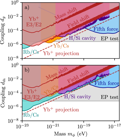
Figure 1: Exclusion plot for the linear scalar DM coupling a) to the gluons $d_{g}$ and b) to the quark masses $d_{\hat{m}}$ as a function of DM mass $m_{\phi}$. Using the field shift effect, limits at the 95% confidence level from long-term measurements of the frequency ratio $\nu_{\textrm{E3}}/\nu_{\textrm{E2}}$ in a single-ion optical clock are shown in dark red. Based on the same experiment, the much weaker limit from the mass shift is shown for reference. The dashed line shows a projection assuming amplitude limits at the $1\times 10^{-18}$-level. The grey and the blue lines depict the strongest EP bound [57] and the bound from various fifth force searches [58], respectively. Bounds from existing spectroscopy experiments are also shown: Rb/Cs [12] (turquoise), Yb/Cs [14] (orange), H/Si [13] (purple).

In Fig. 1, we show the exclusion plot of the scalar UDM coupling $d_{g}$ to gluons and $d_{\hat{m}}$ to the quark masses as a function of DM mass, $m_{\phi}$. Our limits are competitive compared to other spectroscopic limits [12, 14, 13], but importantly rely on a completely different effect, which makes our search complementary to previous results. We set new limits on the coupling $d_{g}$ for masses around $10^{-22}\,$eV. For reference, we also plot the much weaker limits derived from the mass shift. This effect is suppressed here, but it can be used instead of the field shift to probe the nuclear degrees of freedom with optical clocks based on light elements. While bounds from EP tests and fifth-force searches are more stringent than spectroscopic bounds for most masses within the range investigated here, we note that for a non-generic coupling of scalar UDM to the SM content, bounds from the EP-violation and fifth-force experiments may be suppressed by a factor $\mathcal{O}(10^{-3})$ [59, 17].

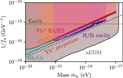
Figure 2: Exclusion plot for the QCD axion coupling $1/f_{a}$ as a function of the axion mass, $m_{a}$. The limits based on the long-term measurements of the frequency ratio $\nu_{\textrm{E3}}/\nu_{\textrm{E2}}$ in a single-ion optical clock are shown in dark red. The dashed line is a projection assuming amplitude limits at the $1\times 10^{-18}$-level. Existing limits based on oscillating neutron electric dipole moment [60] are shown in brown, and theory limits due to density effects of the Earth [61] as a dotted green line. Bounds from existing spectroscopy experiments are also shown: Rb/Cs [12] (turquoise), Yb/Cs [14] (orange), H/Si [13] (purple).

In Fig. 2, we show the parameter space of axion-gluon coupling of Eq. (13) as a function of the axion mass, $m_{a}$. Our limits do not currently exceed those from experiments searching for an oscillating neutron electric dipole moment [60]. However, future investigations using dynamical decoupling techniques [62, 63] can extend the search towards higher masses into a previously experimentally unexplored regime. In this context, we note that the bound associated with Earth [61] is not related to a search for oscillating energy levels. It rather stems from the fact that for small enough $f_{a}$ the Earth-matter density affects the axion potential, driving it away from zero. This bound can possibly be avoided if one introduces a new interaction between the axion and the SM matter fields. In forthcoming work, the analysis in this paper will also be extended to higher frequencies (up to $\sim$100 MHz) based on the experimental data from atomic [64] and molecular [65] spectroscopy.

The measurement can be improved by accumulating more data, or, given a certain measurement time, improving its instability. Since the $\nu_{\textrm{E3}}/\nu_{\textrm{E2}}$ measurement instability is limited by the finite lifetime of the E2 excited state, comparing the E3 clock to a clock with superior stability and suitable sensitivity will lead to an improved search. The projections shown in the plots assume amplitude limits at the $1\times 10^{-18}$ level, which could be obtained with the present $\nu_{\textrm{E3}}$ instability and similar measurement time.

In summary, we show that UDM interacting with the QCD sector leads to oscillations of the nuclear charge radius and consequently of electronic transition frequencies, which can be investigated with high precision in optical clocks. We apply this idea to two transitions in ¹⁷¹Yb⁺. A long-term measurement of the frequency ratio, and the calculated sensitivities, provide constraints on the coupling of UDM to quarks and gluons. While these results only improve the coupling $d_{g}$ for a small mass range, they constitute, to our knowledge, the first investigation of UDM-nuclear couplings using an optical atomic clock comparison. Future investigations based on the derived principle, employing combinations of optical clocks promising larger sensitivity, in particular, those based on highly charged ions [66, 67], are expected to investigate couplings well below the current parameter range.

Supplemental Material

.1 Calculation of $\alpha$ and $\beta$

In the main text, we parameterize the nuclear charge radius dependence on the pion mass, $m_{\pi}$, and decay constant, $f_{\pi}$, through their logarithmic variation as

$$\!\!\!\!\!\frac{\Delta\left<r_{N}^{2}\right>}{\left<r_{N}^{2}\right>}\approx\alpha\frac{\Delta f_{\pi}}{f_{\pi}}+\beta\,\frac{\Delta m_{\pi}^{2}}{m_{\pi}^{2}}\approx\alpha\frac{\Delta\Lambda_{\rm QCD}}{\Lambda_{\rm QCD}}+\beta\,\frac{\Delta m_{\pi}^{2}}{m_{\pi}^{2}}\,,$$ (17)

where, we obtain the right-most equation by using $f_{\pi}\propto\Lambda_{\rm QCD}$ which exists in large $N$ limit [32]. We will use this proportionality throughout this section and use these two quantities interchangeably. In this section we want to estimate the values of $\alpha$ and $\beta$. In general this is not an easy problem. Nuclear radii calculations [68, 69, 70] do not have an explicit dependence on these parameters. Some dependence can be inferred from nucleon radii. For example, the nucleon isovector charge radius has a logarithmic dependence on the pion mass [23] and can be calculated using chiral perturbation theory [24]. A Lattice QCD calculation has considered the nucleon-nucleon potential variation with $m_{\pi}$ [71], but the nucleon mass was changed at the same time so we cannot use this result.

As discussed in [21] (see also [22] and refs therein), the nuclear charge radius is largely determined by the distribution of protons inside the nucleus and the individual charge radii of the nucleons. Thus, we consider two “opposite” models: a “stiff model” in which the nucleons inside the nucleus are tightly packed, and a “puffy” model in which nucleons are held together by a one-pion exchange force, to estimate the nuclear charge radius and the values of $\alpha$ and $\beta$. These opposite models give information about the possible range of $\alpha$ and $\beta$ values.

First we consider a “stiff model”. In this case, as all the nucleons are tightly packed, and the oscillation of the overall nuclear charge radius is tightly linked to the oscillation of the individual nucleons. The charge radius of the nucleus in this model is given by

$$\left<r_{N}\right>\equiv\sqrt{\langle r_{N}^{2}\rangle}\sim A^{1/3}\,\sqrt{\langle r^{2}_{\rm nucleon}\rangle}\,,$$ (18)

with $r_{\rm nucleon}\equiv\sqrt{\langle r^{2}_{\rm nucleon}\rangle}$ being the typical radius of a single nucleon. Below we consider two possible approximation for $r_{\rm nucleon}$, the proton charge radius, $r_{p}\equiv\sqrt{\langle r^{2}_{p}\rangle}$ (as used in the main text), and the nucleon isoscalar charge radius, $r_{s}\equiv\sqrt{\langle r^{2}_{s}\rangle}=\sqrt{\langle r_{p}^{2}\rangle+\langle r_{n}^{2}\rangle}$ with $\langle r_{n}^{2}\rangle$ the squared charge radius of neutron. Using these, the nuclear charge radius $\left<r_{N}\right>$ is

$$\!\!\!\!\!\!\!\left<r_{N}\right> \sim A^{1/3}\sqrt{\langle r_{\rm nucleon}^{2}\rangle}$$ (19)

$$\sim A^{1/3}\begin{cases}\sqrt{\langle r_{p}^{2}\rangle}\,\,{\rm for}\,\,r_{\rm nucleon}=r_{p}\\ \sqrt{\langle r_{p}^{2}\rangle+\langle r_{n}^{2}\rangle}\,\,{\rm for}\,\,r_{\rm nucleon}=r_{s}\end{cases}$$

$$\sim \left(\frac{A}{171}\right)^{1/3}\begin{cases}4.7\,{\rm fm}\,\,\,{\rm for}\,\,r_{\rm nucleon}=r_{p}\\ 4.3\,{\rm fm}\,\,\,{\rm for}\,\,r_{\rm nucleon}=r_{s}\end{cases}$$

where we use $\sqrt{\langle r_{p}^{2}\rangle}=0.84\,{\rm fm}$ and $\langle r_{n}^{2}\rangle=-0.1\,({\rm fm})^{2}$  [72]. In the following we compute the $f_{\pi}$ ($\Lambda_{\rm QCD}$) and $m_{\pi}^{2}$ dependence of $r_{p}$ and $r_{s}$, to obtain $\alpha$ and $\beta$, respectively.

To obtain $\alpha$ and $\beta$, we use the chiral perturbation theory calculation of the nucleon isovector ($\sqrt{\langle r_{v}^{2}\rangle}$) and isoscalar charge radii from [24]. The proton electric form factor $G_{E}^{p}$ is related to isovector and isoscalar electric form factors $G_{E}^{v}$ and $G_{E}^{s}$ as

$$G_{E}^{p}(q^{2})=\frac{1}{2}\left[G_{E}^{v}(q^{2})+G_{E}^{s}(q^{2})\right],$$ (20)

where $q^{2}$ is the transfer four-momentum squared. The proton radius is defined as

$$\left<r_{p}^{2}\right>=\frac{6}{6{G_{E}^{p}}(0)}\frac{G_{E}^{p}(q^{2})}{dq^{2}}\bigg{|}_{q^{2}=0}\,.$$ (21)

The nucleon isovector and isoscalar charge radii are defined analogously which implies $\left<r_{p}^{2}\right>=\left[\left<r_{v}^{2}\right>+\left<r_{s}^{2}\right>\right]/2$. An electric form factor $G_{E}$ is related to the form factors $F_{1}$ and $F_{2}$ via

$$G_{E}(q^{2})=F_{1}(q^{2})+\frac{q^{2}}{4m_{\rm nucleon}^{2}}F_{2}(q^{2})\,.$$ (22)

Thus $\left<r_{v}^{2}\right>=\left<(r_{1}^{v})^{2}\right>+6\,F^{v}_{2}(0)/4m_{\rm nucleon}^{2}$ with $\left<(r_{1}^{v})^{2}\right>\equiv 6\,\left(dF_{1}(q^{2})/dq^{2}\right)|_{q^{2}=0}$.

To estimate the $f_{\pi}$ dependence of $\left<r_{v}^{2}\right>$, we note that $\left<(r_{1}^{v})^{2}\right>$ is inversely proportional to $f_{\pi}^{2}$ [24]. Thus, $\partial\ln\left<(r_{1}^{v})^{2}\right>/\partial\ln f_{\pi}=-2$. To get the $f_{\pi}$ (or $\Lambda_{\rm QCD}$) dependence of the second term of $\left<r_{v}^{2}\right>$, one can write,

$$\Delta\left(\frac{6F^{v}_{2}(0)}{4m_{\rm nucleon}^{2}}\right) = -\frac{3F^{v}_{2}(0)}{m_{\rm nucleon}^{3}}\frac{\partial m_{\rm nucleon}}{\partial\Lambda_{\rm QCD}}\Delta\Lambda_{\rm QCD}$$ (23)

$$= -\frac{2.6\,F^{v}_{2}(0)}{m_{\rm nucleon}^{2}}\frac{\Delta\Lambda_{\rm QCD}}{\Lambda_{\rm QCD}}\,,$$

where we used $\partial\ln m_{\rm nucleon}/\partial\ln\Lambda_{\rm QCD}=0.86$ [73, 74]. Thus, we get

$$\!\!\!\!\!\frac{\Delta\left<r_{v}^{2}\right>}{\left<r_{v}^{2}\right>} \supset -2\left(\frac{\left<(r_{1}^{v})^{2}\right>}{\left<r_{v}^{2}\right>}+\frac{2.6\,F^{v}_{2}(0)}{2\,m_{\rm nucleon}^{2}\left<r_{v}^{2}\right>}\right)\frac{\Delta\Lambda_{\rm QCD}}{\Lambda_{\rm QCD}}$$ (24)

$$\simeq -2\left(1-\frac{0.2\,F^{v}_{2}(0)}{m_{\rm nucleon}^{2}\left<r_{v}^{2}\right>}\right)\frac{\Delta\Lambda_{\rm QCD}}{\Lambda_{\rm QCD}}$$

$$\simeq -2\,\frac{\Delta\Lambda_{\rm QCD}}{\Lambda_{\rm QCD}}\,,$$

where, we used $F^{v}_{2}(0)=3.7$ [24], $m_{\rm nucleon}\sim 940\,{\rm MeV}$, and $\left<r_{v}^{2}\right>=\left<r_{p}^{2}\right>-\left<r_{n}^{2}\right>$ is the difference between the squared charge radii of the proton and the neutron.

One can determine the $m_{\pi}^{2}$ dependence of $\left<(r_{1}^{v})^{2}\right>$ as,

$$\Delta\left<(r_{1}^{v})^{2}\right>\supset\frac{\partial\left<(r_{1}^{v})^{2}\right>}{\partial m^{2}_{\pi}}\Delta m^{2}_{\pi}=-\frac{1+5g_{A}^{2}}{16\pi^{2}f_{\pi}^{2}}\frac{\Delta m^{2}_{\pi}}{m^{2}_{\pi}}\,,$$ (25)

where we have ignored the $\Delta$ coupling dependence. We can obtain the $m_{\pi}^{2}$ dependence of the second term of $\left<r_{v}^{2}\right>$ as,

$$\Delta\left(\frac{6F^{v}_{2}(0)}{4m_{\rm nucleon}^{2}}\right) = -\frac{3F^{v}_{2}(0)}{m_{\rm nucleon}^{3}}\frac{\partial m_{\rm nucleon}}{\partial m_{\pi}^{2}}\Delta m_{\pi}^{2}$$ (26)

$$= -\frac{0.7}{m_{\rm nucleon}^{2}}\frac{\Delta m_{\pi}^{2}}{m_{\pi}^{2}}\,,$$

where we have used $\partial\ln m_{\rm nucleon}/\partial\ln m_{\pi}^{2}\simeq 0.06$ [10] and $F^{v}_{2}(0)=3.7$ [24]. Thus ignoring the $\Delta$ coupling dependence, we obtain the $m_{\pi}$ dependence of $\left<r_{v}^{2}\right>$ as,

$$\frac{\Delta\left<r_{v}^{2}\right>}{\left<r_{v}^{2}\right>}\supset-\frac{1}{\left<r_{v}^{2}\right>}\left(\frac{1+5g_{A}^{2}}{16\pi^{2}f_{\pi}^{2}}+\frac{0.7}{m_{\rm nucleon}^{2}}\right)\frac{\Delta m^{2}_{\pi}}{m^{2}_{\pi}}\,.$$ (27)

To obtain the $m_{\pi}^{2}$ and $\Lambda_{\rm QCD}$ dependence of $\left<r_{s}^{2}\right>$, we write $\left<r_{s}^{2}\right>$ following the notation of the journal version of [24] as,

$$\left<r_{s}^{2}\right>=6\left(-\frac{\tilde{B_{1}}}{(4\pi f_{\pi})^{2}}+\frac{\kappa_{s}}{4m_{\rm nucleon}^{2}}\right)\,,$$ (28)

where, $\kappa_{s}=F^{s}_{2}(0)=-0.12$ and $\tilde{B_{1}}=-3.5$ [24]. We obtain the $\Lambda_{\rm QCD}$ dependence of $\left<r_{s}^{2}\right>$ as,

$$\frac{\Delta\left<r_{s}^{2}\right>}{\left<r_{s}^{2}\right>} \supset -2\left(1-\frac{0.2\,\kappa_{s}}{m_{\rm nucleon}^{2}\left<r_{s}^{2}\right>}\right)\frac{\Delta\Lambda_{\rm QCD}}{\Lambda_{\rm QCD}}$$ (29)

$$\simeq -2\,\frac{\Delta\Lambda_{\rm QCD}}{\Lambda_{\rm QCD}}\,,$$

where, we used $\left<r_{s}^{2}\right>=\left<r_{p}^{2}\right>+\left<r_{n}^{2}\right>$.

Ignoring the 3-pion processes [75] which are suppressed, we can calculate the $m_{\pi}^{2}$ dependence of $\left<r_{s}^{2}\right>$ as,

$$\frac{\Delta\left<r_{s}^{2}\right>}{\left<r_{s}^{2}\right>} \supset -\frac{3\times(0.06)\,\kappa_{s}}{m_{\rm nucleon}^{2}\left<r_{s}^{2}\right>}\frac{\Delta m_{\pi}^{2}}{m_{\pi}^{2}}$$ (30)

$$\simeq 2\times 10^{-3}\,\frac{\Delta m_{\pi}^{2}}{m_{\pi}^{2}}\,,$$

where we use $\partial\ln m_{\rm nucleon}/\partial\ln m_{\pi}^{2}\simeq 0.06$. Using $\left<r_{p}^{2}\right>=\left[\left<r_{v}^{2}\right>+\left<r_{s}^{2}\right>\right]/2$, we get the $\Lambda_{\rm QCD}$ dependence of $\left<r_{p}^{2}\right>$ as,

$$\frac{\Delta\left<r_{p}^{2}\right>}{\left<r_{p}^{2}\right>} = \left(\frac{\left<r_{v}^{2}\right>}{2\left<r_{p}^{2}\right>}\frac{\Delta\left<r_{v}^{2}\right>}{\left<r_{v}^{2}\right>}+\frac{\left<r_{s}^{2}\right>}{2\left<r_{p}^{2}\right>}\frac{\Delta\left<r_{s}^{2}\right>}{\left<r_{s}^{2}\right>}\right)$$ (31)

$$\supset -2\,\frac{\Delta\Lambda_{\rm QCD}}{\Lambda_{\rm QCD}}$$

where, to obtain the last line we used Eq. (24) and Eq. (29). Thus, we obtain $\alpha=-2$ both for $r_{\rm nucleon}=r_{p}$ and $r_{\rm nucleon}=r_{s}$.

Similarly using Eq. (27) and Eq. (30), we obtain the $m_{\pi}^{2}$ dependence of $\left<r_{p}^{2}\right>$ as,

$$\frac{\Delta\left<r_{p}^{2}\right>}{\left<r_{p}^{2}\right>} \supset -\frac{1}{2\left<r_{p}^{2}\right>}\left(\frac{1+5g_{A}^{2}}{16\pi^{2}f_{\pi}^{2}}+\frac{0.68}{m_{\rm nucleon}^{2}}\right)\frac{\Delta m^{2}_{\pi}}{m^{2}_{\pi}}$$ (32)

$$\simeq -0.2\,\frac{\Delta m^{2}_{\pi}}{m^{2}_{\pi}}\,,$$

where we have used $g_{A}^{2}=(1.27)^{2}$ [72]. Thus $\beta=-0.2$ for the case of $r_{\rm nucleon}=r_{p}$ and $\beta=2\times 10^{-3}$ for the case of $r_{\rm nucleon}=r_{s}\,$. Including the $\Delta$ coupling in the calculations above changes the value of $\beta$ for $r_{p}$ by less than 10%, well within our rounding error.

Next we consider a “puffy model”, and calculate the inter-nucleon distance by one-pion exchange processes. As given in [76], the one-pion exchange Bonn potential can be written as

$$V(r)=\,\, -\frac{g_{\pi NN}^{2}}{16\pi\,m_{\rm nucleon}^{2}}e^{-m_{\pi}r}\left[(\vec{\sigma_{1}}\cdot\vec{\sigma_{2}})\left(\frac{m_{\pi}}{r^{2}}+\frac{1}{r^{3}}\right)\right.$$ (33)

$$-\left.(\vec{\sigma_{1}}\cdot\hat{r})(\vec{\sigma_{2}}\cdot\hat{r})\left(\frac{m_{\pi}^{2}}{r}+\frac{3m_{\pi}}{r^{2}}+\frac{3}{r^{3}}\right)\right]\,,$$

where, $m_{\rm nucleon}$ is the mass of the nucleon, $\sigma_{1}$ and $\sigma_{2}$ denote the spin of nucleons arising due to the pseudo-scalar nature of the force mediator (pion in our case), and $g_{\pi NN}$ is the effective pion-nucleon coupling constant given as $g_{\pi NN}^{2}/(4\pi)\simeq 14.9$ [76, 77]. The Bonn potential is minimized for an anti-parallel spin configuration i.e. when $(\vec{\sigma_{1}}\cdot\vec{\sigma_{2}})=-1$ and $(\vec{\sigma_{1}}\cdot\hat{r})(\vec{\sigma_{2}}\cdot\hat{r})=-1$. For the anti-parallel spin configuration, the potential described in Eq. (33) can be written as

$$\!\!\!\!V(r)=-\frac{g_{\pi NN}^{2}}{16\pi\,m_{\rm nucleon}^{2}r^{3}}e^{-m_{\pi}r}\left[2+2m_{\pi}r+m_{\pi}^{2}r^{2}\right]\,.$$ (34)

In the regime $r\gg 1/m_{\pi}$ the $1/r$ term becomes dominant and the potential can be written as

$$V(r)\simeq-\frac{g_{\pi NN}^{2}m_{\pi}^{2}}{16\pi\,m_{\rm nucleon}^{2}r}\,.$$ (35)

With all these simplifications, we can calculate the typical size of a two nucleon bound state with a reduced mass of $m_{\rm nucleon}/2$ as

$$a_{\rm eff}\sim\frac{32\pi\,m_{\rm nucleon}}{g_{\pi NN}^{2}m_{\pi}^{2}}\sim 5\,{\rm fm}\,,$$ (36)

where we used $m_{\rm nucleon}\sim 940\,{\rm MeV}$, and $m_{\pi}\sim 140\,{\rm MeV}$. In this model the typical distance between two nucleons is much larger than individual nucleon radii. The nuclear charge radius, $\langle r_{N}\rangle$, is

$$\langle r_{N}\rangle\equiv\sqrt{\langle r_{N}^{2}\rangle} \sim A^{1/3}\,a_{\rm eff}\sim A^{1/3}\,\frac{32\pi\,m_{\rm nucleon}}{g_{\pi NN}^{2}m_{\pi}^{2}}$$ (37)

$$\sim 28\,{\rm fm}\,\left(\frac{A}{171}\right)^{1/3}.$$

Thus we obtain $\beta=-2$. Using $\partial\ln m_{\rm nucleon}/\partial\ln\Lambda_{\rm QCD}=0.86$, we get $\alpha=1.72$.

We see that the two models yield quite different values of $\alpha$ and $\beta$. This highlights that the dependence of $\langle r_{N}\rangle$ on $\Lambda_{\rm QCD}$ and $m_{\pi}^{2}$ requires further study. For the main text we would like to choose a default model.

As discussed in the main text, the nuclear charge radius of Yb is $\langle r_{N}\rangle\approx 5.3\,{\rm fm}$ [51]. Yb charge radius estimation using the stiff model is $4.3-4.7$ fm (Eq. (19)), whereas using the puffy model we obtained a charge radius of $28\,{\rm fm}$ (Eq. (37)). Note that the stiff model estimate is within $20\%$ accuracy of the measured value as quoted above. Furthermore, in the stiff model, we calculated the $m_{\pi}^{2}$ and $f_{\pi}$ dependence of the nuclear charge radius using chiral perturbation theory which provides a good framework for low energy QCD calculations. Therefore the stiff model is used in the main text to make the exclusion plots. Both choices for $r_{\rm nucleon}$ yield $\langle r_{N}\rangle$ close to the measured one. We choose to use the proton charge radius, $r_{p}$, as an approximation to $r_{\rm nucleon}$, as it incorporates the explicit logarithmic dependence on the pion mass, one of the truly model-independent facts about the charge radius. A detailed investigation involving lattice simulation may result in a more precise estimate of the $\alpha$ and $\beta$ coefficients which is beyond the scope of the current work.

.2 Order of magnitude estimate of $K_{\rm FS}$

We can obtain an order of magnitude estimate of $K_{\rm FS}$ by using quantum mechanical first order perturbation theory and the fact that the nuclear size is small compared to the atomic size. The energy level shift is [78]

$$(\Delta E)_{\rm FS}=\frac{2\pi}{3}\left|\psi(0)\right|^{2}Z\alpha\left<r_{N}^{2}\right>,$$ (38)

where $\psi$ is the wave function of the state, and $\alpha$ denotes the fine structure constant here. From [79] we have for an $s$-wave of a valence electron in a heavy, neutral, multi-electron atom, $\left|\psi_{s}(0)\right|^{2}=Z/a_{0}^{3}$, where $a_{0}\approx 0.53\cdot 10^{5}$ fm is the Bohr radius. In $\hbar=1,c=1$ units, $1\mbox{ fm}^{-1}=3\cdot 10^{14}\mbox{ GHz}$. For Yb $Z=70$, which gives an energy shift of

$$\Delta E\approx\frac{2\pi}{3}Z^{2}\alpha\frac{\left<r_{N}^{2}\right>}{a_{0}^{3}}\approx 150\frac{\mbox{GHz}}{\mbox{fm}^{2}}\left<r_{N}^{2}\right>\,.$$ (39)

Up to a sign and within an order of magnitude this agrees with the calculated values of $K^{\nu}_{\rm FS}$. We emphasize that this is only an order of magnitude estimate and it does not replace the detailed calculation in the main text.

.3 Order of magnitude estimate of the field shift and the mass shift

In this section we estimate the energy level shift due to the finite nuclear mass (mass shift) and finite nuclear size (field shift) for the $ns$ energy level of a valence electron in a heavy, neutral, multi-electron atom.

Recall, the mass shift for a hydrogen like atom can be estimated as [79]

$$\Delta E_{{\rm MS},n}=\frac{m_{e}^{2}\alpha^{2}}{2\,m_{N}\,n^{2}}=\frac{1}{2\,m_{N}\,a_{0}^{2}\,n^{2}}\,,$$ (40)

where, $m_{N}$ is the mass of the nucleus and can be approximated as $m_{N}\sim A\,m_{\rm nucleon}\,$. In the previous section, we estimated the field shift. Combining Eq. (39) with the “stiff model” of the nucleus in which we obtained $\left<r_{N}^{2}\right>\sim A^{2/3}r_{p}^{2}$, the field shift for the $ns$ level can be written as

$$\Delta E_{{\rm FS},n}=\frac{2\pi}{3\,n^{3}}\frac{Z^{2}\alpha}{a_{0}^{3}}A^{2/3}r_{p}^{2}\,.$$ (41)

Since $E_{{\rm MS},n}\sim A^{-1}$ and $E_{{\rm FS},n}\sim A^{2/3}$, for large enough $A$ the field shift dominates over the mass shift. By using simplifications such that $Z\sim A/2$ and using $r_{p}^{2}\sim(0.84\,\rm fm)^{2}$ we obtain that the field shift dominates for

$$A\gtrsim\left(\frac{3\,n\,a_{0}}{\pi\,\alpha\,r_{p}^{2}\,m_{\rm nucleon}}\right)^{3/11}\sim 86\left(\frac{n}{6}\right)^{3/11}.$$ (42)