Quantum anomaly detection in the latent space of proton collision events at the LHC

Abstract

We propose a new strategy for anomaly detection at the LHC based on unsupervised quantum machine learning algorithms. To accommodate the constraints on the problem size dictated by the limitations of current quantum hardware we develop a classical convolutional autoencoder. The designed quantum anomaly detection models, namely an unsupervised kernel machine and two clustering algorithms, are trained to find new-physics events in the latent representation of LHC data produced by the autoencoder. The performance of the quantum algorithms is benchmarked against classical counterparts on different new-physics scenarios and its dependence on the dimensionality of the latent space and the size of the training dataset is studied. For kernel-based anomaly detection, we identify a regime where the quantum model significantly outperforms its classical counterpart. An instance of the kernel machine is implemented on a quantum computer to verify its suitability for available hardware. We demonstrate that the observed consistent performance advantage is related to the inherent quantum properties of the circuit used.

I Introduction

Quantum Machine Learning (QML) is a nascent field at the intersection of quantum information processing and machine learning [1, 2, 3, 4, 5, 6, 7, 8] that has the potential to revolutionise the way we solve problems in High Energy Physics (HEP). There is a growing number of studies investigating this new paradigm, its possible advantages over classical computing, and its applicability to varied real-life problems. [9, 10, 11, 12, 8, 13].

The use of quantum computing techniques on HEP problems was introduced by Ref. [14], where the task of training a classifier for photon selection in a search for the Higgs boson was framed as a quantum annealing problem. Since then, QML algorithms have been examined for event reconstruction tasks [15, 16, 17, 18, 19] and classification problems [20, 21, 22, 23, 24] in HEP. All these problems belong to the realm of supervised learning, in which the training process is guided by comparing the algorithm output to the ground truth, provided with the training dataset. A natural evolution of this line of research is the extension of QML techniques to unsupervised problems, i.e., to learning processes on unlabeled data. This is the case of Refs. [25, 26], where anomaly detection quantum algorithms have been applied to low-dimensionality datasets.

In this work, we investigate the use of a classical-quantum pipeline, in which a high-dimensional dataset is projected to a low-dimensional latent space via a classical autoencoder and a set of unsupervised quantum algorithms are trained on the latent-space features. We consider the problem of searching for new physics processes in Large Hadron Collider (LHC) events as an anomaly detection problem. Our approach aims to implement a prototype pipeline that is able to process realistic datasets and could be eventually deployed at the LHC to assist scientific discovery (see Fig. 1). Similar problems have been considered on low-dimensional datasets in Ref. [25, 26], where different approaches have been followed.

After the discovery of the Higgs boson by the ATLAS [27, 28] and CMS [29, 30] collaborations, one of the main goals of the LHC physics program is the search for new phenomena (new particles, new forces, new symmetries, etc.) that would answer some of the open questions associated with the Standard Model (SM) of particle physics, the theory that describes our understanding of the fundamental constituents of the universe: why are the known forces in nature characterized by largely different energy scales? What is the mechanism that generates neutrino masses? What is the origin of Dark Matter and Dark Energy? To answer these questions, proton beams are accelerated in the LHC up to an energy of 6.75 TeV and made to collide. These collisions happen at energies that were typical of particle collisions in the early universe. By studying them in a controlled environment, physicists aim to understand post-big-bang physics and possibly highlight the difference between observations and SM predictions.

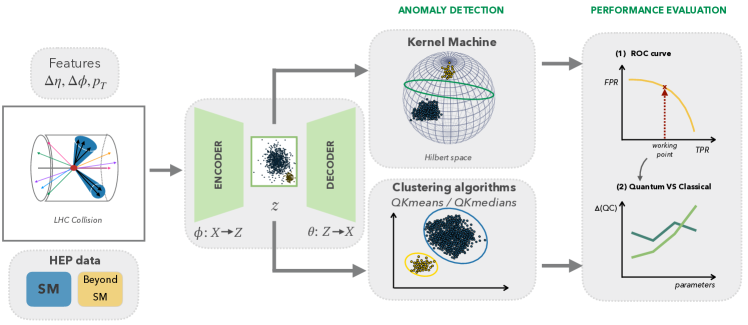
Figure 1: Classical-quantum pipeline. LHC collision data (simulation) are passed through an autoencoder for dimensionality reduction followed by the quantum anomaly detection models: unsupervised quantum kernel machine and clustering algorithms (QK-means/QK-medians). Each jet contains 100 particles, each particle is described by three features $(\Delta\eta,\Delta\phi,p_{T})$ where $\Delta$ represents a distance from the jet axis. Hence, a dijet collision event is described by 300 features. The quantum models are trained on Standard Model data and learn to recognise anomalies in unseen data. All models are evaluated by calculating the Receiver Operating Characteristic (ROC) curve and metrics appropriate for anomaly detection tasks and are compared to their classical counterparts (see Sec. IV). The depicted curves are for illustrative purposes.

These searches for Beyond Standard Model (BSM) physics are typically model-dependent. In this context, a signal is defined as a specific process described by the chosen BSM scenario. The background is defined as any SM process that generates a similar detector signature as that of a BSM process. In the recent past, the use of supervised Machine Learning (ML) algorithms has become prominent. These ML algorithms are typically trained on labeled data from Monte Carlo (MC) simulations and applied to experimental data.

This model-dependent approach exploits at best the solid understanding of the physics associated with the postulated signal and the known background processes, and typically reaches remarkable signal-to-background discrimination power, as in the case of the discovery of the Higgs boson. However, the need to postulate a priori the signal of interest has an intrinsic drawback: searches based on a given signal assumption are typically less sensitive to other kinds of signals. If an unexpected signature is present in the data, it might not be identified due to the inherent bias of the study toward the chosen signal hypothesis.

To overcome this drawback, one could follow an unsupervised approach, in which the search for new physics is rephrased as Anomaly Detection (AD). These types of algorithms can be employed for BSM searches relying minimally on specific new physics scenarios. In this context, anomalies are defined as any event in the data that deviates from the SM predictions. Anomaly detection for new physics searches in multijet events has been proposed in Refs. [31, 32] and then refined in many other studies (see Refs. [33, 34] for recent reviews). This strategy has been introduced as a new way to select events in real time [35] and it has been successfully adapted in a proof-of-concept study with real data [36]. Recently, the ATLAS collaboration released two searches with weakly supervised [37] and unsupervised [38] techniques.

Unsupervised algorithms for AD rely on less information than supervised methods since signal vs. background characterization through labels is not explored. On the other hand, thanks to their increased generalizability to other BSM signatures, AD techniques offer qualitative advantages with respect to traditional methods, which can contribute to expand the physics reach of the LHC experiments. This is why AD algorithms for HEP offer an interesting scientific problem to investigate, particularly with unsupervised QML techniques. Quantum algorithms have many specific aspects that differentiate them from classical solutions proposed in the literature, typically based on deep neural networks trained on large datasets. In particular, QML provides advantages in terms of computational complexity [39, 10], generalization with few training instances [12], or the ability to uncover patterns unrecognisable to classical approaches [11, 40].

Similar to other prototype studies of AD techniques in HEP [33], we consider the problem of looking for new exotic particles decaying to jet pairs. Jets are sprays of close-by particles originating from a shower of hadrons, following the production of quarks and gluons in LHC collisions. Traditional jets have a one-prong cone shape and are copiously produced in so-called Quantum Chromodynamics (QCD) multijet events, the most frequent processes occurring in LHC collisions. At the LHC, multi-prong jets could emerge from all-quark decays of heavy particles manifesting as a peak in the dijet-mass ($m_{jj}$) distribution (a resonance). However, this peak could be obscured by the huge multijet background and an AD technique could be used to suppress the background and make the resonant peak emerge.

In our setup, data are mapped to a latent representation of reduced dimensionality using an autoencoder model. Our quantum algorithms are trained to extract a metric of typicality from the values of the latent-space quantities after data encoding. We develop an unsupervised quantum kernel machine and two quantum clustering algorithms to identify latent representations of BSM processes in a model-independent setting.

The discrimination power of the quantum models is assessed using a metric tailored to anomaly detection tasks. In the case of kernel-based anomaly detection, for the first time in HEP, we identify an instance of significant and consistent performance advantage of the quantum model over its classical counterpart. The statistical robustness of these results is systematically studied across parameters of interest, as discussed in Sec. IV. Furthermore, we demonstrate that the observed performance advantage of the QML model is related to intrinsic quantum properties of the kernel. Specifically, the dimensionality of the quantum Hilbert space, that is the number of qubits, the expressibility, and the entanglement capability of the designed data encoding circuit. These metrics are used in a data-dependent setting suitable for this work, extending Ref. [41], as detailed in App. B.

This paper is structured as follows. In Section II, we present the studied HEP processes and the method for dimensionality reduction. Section III defines the QML algorithms for anomaly detection. In Section IV, we present and interpret the results of the proposed quantum models using metrics appropriate for anomaly detection tasks. Our conclusions are discussed in Section V.

II Data

The dataset used for this study consists of proton-proton collisions simulated at a center-of-mass energy $\sqrt{s}=13$ TeV, produced with pythia [42]. The following BSM processes are considered as anomalies to benchmark the model performance. These processes are representative of new-physics scenarios that the LHC experiments are sensitive to.

• Production of narrow Randall-Sundrum gravitons [43] decaying to two $W$-bosons (Narrow $G\to WW$). The width of the Randall-Sundrum (RS) graviton is set to a negligible value, fixing the $\kappa\times m_{G}$ parameter [44] in pythia to 0.01.

• Production of broad Randall-Sundrum gravitons [43] decaying to two $W$-bosons (Broad $G\to WW$). The graviton width-to-mass ratio is fixed by choosing $\kappa\times m_{G}=2.5$, which results in a width-to-mean ratio $\sim 35\%$ for $m_{\mathrm{jj}}$ after detector effects.

• Production of a scalar boson $A$ decaying to a Higgs and a Z bosons ($A\to HZ$). Higgs bosons are then forced to decay to $ZZ$, resulting in a $ZZZ$ final state.

The resonance masses are varied between 1500 GeV and 4500 GeV, in steps of 1000 GeV. All the $W$ and $Z$ bosons are forced to decay to quark pairs, resulting in all-jet final states. SM events are generated emulating QCD multijet production at the LHC, by far the most abundant process in a sample of all-jet events.

Events are processed with DELPHES library [45] to emulate detector effects, using the distributed CMS detector description. The effect of additional simultaneous proton collisions (in-time pileup) is included. This is achieved by overlapping low-momentum collision events, sampled from a set of simulated LHC collisions, with the primary interaction vertex. The number of overlayed events varies according to a Poisson distribution centered at 40, resembling the in-time pileup recorded at the LHC at the end of 2018. The QCD multijet dataset size corresponds to an integrated luminosity of $64\mbox{$\,\text{fb}^{-1}$}$, comparable to running the LHC for about one year.

Detector coordinates are specified with respect to the Cartesian coordinate system with the $z$ axis oriented along the beam axis and $x$ and $y$ axes defining the transverse plane. The azimuthal angle $\phi$ is computed from the $x$-axis. The polar angle $\theta$, measured from the positive $z$-axis, is used to compute the pseudorapidity $\eta=-\log(\tan(\theta/2))$. The transverse momentum $p_{\mathrm{T}}$ is defined as the projection of the momentum of a particle or a jet on the plane perpendicular to the beam axis. We fix units such that $c=\hbar=1$.

Events are processed using the particle-flow algorithm [45]. Jets are clustered from reconstructed particles running the anti-$k_{\mathrm{T}}$ [46] clustering algorithm with jet-size parameter $R=0.8$ in FastJet [47]. Dijet events are selected requiring two jets with $p_{\mathrm{T}}>200\,\text{GeV}$ and within $|\eta|<2.4$. In order to emulate the effect of a typical LHC online event selection, only jet pairs with invariant mass $m_{\mathrm{jj}}>1260\,\text{GeV}$ are considered.

Each event is represented by its two highest-$p_{\mathrm{T}}$ jets. Each jet is represented by a list of constituents, built considering the 100 highest-$p_{\mathrm{T}}$ particles, reconstructed by the particle-flow algorithm and contained in a cone of radius $\Delta R=\sqrt{\Delta\phi^{2}+\Delta\eta^{2}}<0.8$ from the jet axis. Particles are ordered according to their decreasing $p_{\mathrm{T}}$ value. Zero padding is used to extend particle sequences shorter than 100 particles. Each particle is represented by its $p_{\mathrm{T}}$ and its $\eta$ and $\phi$ distance from the jet axis. In its raw format, a jet is then represented as a $100\times 3$ matrix.

A jet training dataset is defined using the so-called dijet $\Delta\eta$ sideband, requiring the pseudorapidity separation between the two highest-$p_{\mathrm{T}}$ jets in the event $|\Delta\eta_{jj}|>1.4$. This kinematic region is largely populated by QCD multijet events and any potential signal contamination by BSM processes involving high-energy collisions is typically negligible. The classical autoencoder is trained on this dataset to learn the compression of the input data to the latent space.

Quantum and classical AD algorithms are trained on QCD multijet events in a signal region, defined requiring $|\Delta\eta_{jj}|\leq 1.4$. Their performance is assessed using events from the benchmark models belonging to the same signal region.

Dimensionality reduction.

Direct loading and processing of such datasets on current near-term, noisy, quantum devices is typically not possible due to the limited number of qubits and their small decoherence times [48]. To address this challenge, we develop a convolutional autoencoder (AE) that maps events into a latent representation of reduced dimensionality (architecture presented in App. A). The AE is designed to act at per-particle level in its 1D convolutional input layer, to be appropriately biased to the structure of our jet data, similarly to the model in Ref. [49]. The model is trained to compress particle jet objects individually, using background QCD data in the sideband region, without access to truth labels. Hence, for our analysis, the reduced dijet datasets have $2\ell$ features, where $\ell$ is the dimension of the latent representation for each jet.

Most studies of QML applications in HEP and beyond, rely on pre-processing methods to reduce the dimensionality of features. Even though such a task is presently required for a high-dimensional dataset, it can introduce biases that negatively affect the performance of the QML models. Many studies report similar performance between quantum and classical algorithms [20, 24, 23, 22, 21, 25, 26]. We expect that, quantum models require access to the unprocessed data, ideally right after measurement by the detector, to exploit correlations and potentially achieve higher performance. The more post-processing steps there are after the measurement, the higher the probability of losing fundamental quantum correlations leading to suboptimal performance of the quantum algorithms. For this reason, we work exclusively with low-level data, that is, the four-momenta of the particles. The autoencoder is applied to the input data, which is still a form of classical post-processing. However, unlike PCA or manual feature selection, autoencoders have the potential of retaining, at least partially, the non-linear correlations in the latent space.

III Methods for quantum anomaly detection

The developed QML algorithms are trained to define a metric of typicality for QCD jets, which can then be used to identify anomalies. We consider two categories of quantum models: kernel machines and clustering algorithms.

Kernel Machines.

Support Vector Machines (SVM) are powerful models that can serve as the kernel-based model blueprint in supervised learning [50]. Quantum Support Vector Machines (QSVM) are defined over an input feature vector space $\mathcal{I}$ and a set of data labels $\mathcal{Y}=\{-1,1\}$ by constructing a quantum kernel [4, 6]. Supervised QSVM have been employed for classification tasks in HEP [21, 24], reaching similar performance to their classical counterparts. We extend this idea to the unsupervised learning setting, where we separate expected (SM) and anomalous (BSM) events. Given the quantum feature map $\rho:\;\mathcal{I}\mapsto\mathcal{H}$, that maps the HEP events to the Hilbert space $\mathcal{H}$ of $n$ qubits, we can define the quantum kernel using the Hilbert-Schmidt inner product

$$k(x_{i},x_{j})\coloneqq\text{tr}[\rho(x_{i})\rho(x_{j})]=\left|{\braket{0}{U^{\dagger}(x_{i})U(x_{j})}{0}}\right|^{2},$$ (1)

where the quantum feature map is identified as the density matrix operator $\rho(x_{i})\coloneqq U(x_{i})\ket{0}\bra{0}U^{\dagger}(x_{i}),$ where $U(\cdot)$ corresponds to a data encoding quantum circuit that represents the quantum feature map, and $\ket{0}=\ket{0}^{\otimes n}\in\mathcal{H}$. The unsupervised kernel machine is trained to find the hyperplane that maximizes the distance of the training data from the origin of the feature vector space, similar to the classical algorithm [51]. We optimize the objective function on a classical device, while the kernel matrix elements $K_{ij}=k(x_{i},x_{j})$ are sampled from a quantum computer.

Different strategies to embed data into quantum states have been studied in literature [6, 52, 7]. For this study, we design a novel quantum feature map implemented by the quantum circuit depicted in Fig. 2a, taking into account the following properties. The data embedding ansatz maps two input features to the two physical degrees of freedom of each qubit via unitary rotation gates and employs nearest-neighbors entanglement between qubits. The encoding gates are repeated, by permuting the rotation angles to which the features correspond, introducing non-trivial interactions between features, and avoiding encoding different features along the same axis of rotation. The quantum circuit, as a whole, can be repeated to increase the expressibility and entanglement capability of the feature map. The number of repetitions is treated as a parameter to tune the balance between the expressiveness of the kernel machine and its performance, as further discussed in Sec. IV; for more details see App. B, C, and D. The quantum circuit is designed to be hardware-efficient, i.e., it is compact and takes into account the topology of superconducting qubits. A hardware implementation of the algorithm is presented in Sec. IV, in absence of any error mitigation, to demonstrate the robustness and feasibility of the circuit.

Clustering algorithms.

The Quantum K-means (QK-means) and Quantum K-medians (QK-medians) are unsupervised clustering algorithms [53]. In resemblance to their classical counterparts, these algorithms partition a dataset of $N$ samples $x\in\mathbb{R}^{M}$ into $k$ clusters based on a distance metric. For both clustering models, we perform amplitude encoding to map the inputs to normalized quantum states, requiring $n=\log_{2}(2f)$ qubits for a dataset of $f$ features. We follow two different strategies for the cluster assignment.

Quantum K-means algorithm.

In the case of the QK-means model, each cluster center is defined as the mean of the training samples assigned to it in the previous iteration. We use a quantum optimization algorithm [54, 55] based on Grover’s search [56], with a time complexity of $\mathcal{O}(\sqrt{k})$, to find the closest cluster to each training sample. Given two input vectors u and v, the quantum states $\ket{\psi}$ and $\ket{\phi}$ are prepared as

$$\ket{\psi}=\frac{1}{\sqrt{2}}(\ket{0}\ket{u}+\ket{1}\ket{v}),\quad\ket{\phi}=\frac{1}{\sqrt{Z}}(|u|\ket{0}-|v|\ket{1}),$$ (2)

where Z = $|u|^{2}+|v|^{2}$. Subsequently, a controlled swap test (Fig. 2b) is performed to calculate the overlap $\braket{\phi}{\psi}$. Then, the distance $D$, proportional to the Euclidean distance is calculated as

$$D=2Z|\braket{\phi}{\psi}|^{2}.$$ (3)

To find the closest cluster, the minimization technique starts by selecting a random threshold picked from the vector of distances and constructing a threshold-oracle (Eq. 4) as a linear combination of m simpler oracles, where $m\leq k$. A simple oracle is a unitary operator performing $\ket{x}\ket{q}\xrightarrow{\raisebox{-1.72218pt}[0.0pt][0.0pt]{\tiny{$O$}}}\ket{x}\ket{q\oplus f(x)}$ where $\ket{x}$ is an array of indices, $\oplus$ is the addition modulo 2 and $\ket{q}$ is the oracle control qubit. The threshold oracle

$$O=\delta(t_{0}-1)O_{0}+\delta(t_{1}-1)O_{1}+\cdots+\delta(t_{m}-1)O_{m}$$ (4)

marks multiple entries by linking a set of simple oracles through the $\delta$ function centered at threshold $t_{i}$ where oracle $O_{i}$ marks all inputs $\{x\}$ for which $f(x)<t_{i}$ and where $f$ returns the value of the distance array at index $x$. The minimization procedure runs for $\sqrt{2^{|k|}}$ iterations, applying the Grover search algorithm which sets the most probable output as the new threshold for the next iteration. As the last step, we calculate the mean of the centers in a classical way. The procedure is repeated until convergence is reached up to a tolerance $\varepsilon$.

Quantum K-medians algorithm.

For the QK-medians, we choose a shallower quantum circuit for distance calculation and a hybrid minimization procedure for finding the cluster median. A quantum circuit [53] uses destructive inference probabilities to find a distance proportional to the Euclidean distance between N-dimensional points. Firstly, classical inputs are encoded into a quantum state in a state preparation procedure using amplitude encoding (explained in section IV-C in Ref. [53]). Then, one Hadamard gate is applied to the most significant qubit (MSQB) and destructive inference probabilities are obtained by measuring the MSQB in state |1$\rangle$. This circuit only prepares one quantum state and applies only one quantum gate, making it less complex than the circuit for computing distances in the QK-means algorithm. After the distance calculation, all points are assigned to a specific cluster using a hybrid minimization procedure, consisting of quantum distance calculation and a classical iterative algorithm for finding the median. The median, being the point with the minimal distance to all other points in the cluster, is found iteratively by searching in the direction of more concentrated points. The iterative procedure is based on the algorithm from Ref. [57]. The full procedure is repeated until cluster medians converge to a fixed point for a tolerance $\varepsilon$. For clustering models the number of clusters, $k$, is set to the value of 2.

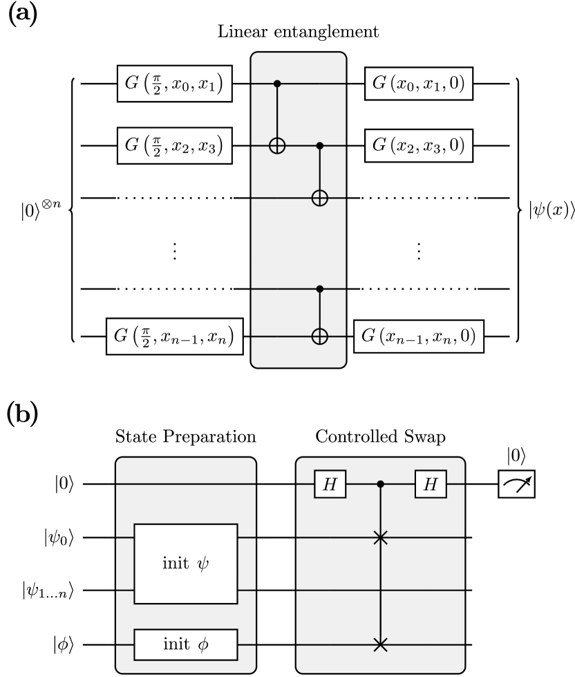
Figure 2: The quantum circuits. (a) Data encoding circuit, $U(x)$, that implements the feature map of the unsupervised kernel machine for a data point $x$, where $G(\theta,\phi,\lambda)\in\text{SU(2)}$ is a general 1-qubit gate, and $x_{i}$, for $i=0,1,\dots,n$, denotes the elements of the input feature vector $x$. (b) Quantum distance calculation circuit used to compute the similarity between an input sample and a cluster center in the QK-means algorithm.

IV Results

We assess the performance of the proposed quantum algorithms in terms of their ability to detect new-physics events. Quantitatively, we compute the Receiver Operating Characteristic (ROC) curve and the corresponding Area Under the Curve (AUC). Even though the AUC provides an overview of the model performance, it is not an informative metric when only a region of the ROC curve is of practical interest. Such is the case for anomaly detection in HEP. Concretely, we focus on specific values of True Positive Rate (TPR) and their corresponding False Positive Rate (FPR). In HEP nomenclature these metrics are called signal and background efficiencies and are denoted by $\varepsilon_{s}$ and $\varepsilon_{b}$, respectively. We consider typical working points in physics analyses at the LHC, where $\varepsilon_{s}=0.6,0.8$. Furthermore, to quantify potential quantum advantage in terms of model performance we define the following metric,

$$\Delta_{\text{QC}}(\varepsilon_{s})=\frac{\varepsilon^{-1}_{\text{b}}(\varepsilon_{s};Q)}{\varepsilon^{-1}_{b}(\varepsilon_{s};C)},$$ (5)

where $\varepsilon^{-1}_{b}(\varepsilon_{s};\cdot)$ is the background rejection ($\mathrm{FPR}^{-1}$) at a working point $\varepsilon_{s}$, given a specific quantum (Q) or classical (C) model.

We systematically study the performance of our models across three parameters of interest using ideal simulations of quantum circuits. Firstly, we evaluate the performance using different new physics anomalous signatures, described in Sec. II. The second parameter of interest is the latent space dimensionality, evaluated for $\ell\in\{4,\,8,\,16\}$ for all models, and additionally $\ell=32$ for the clustering algorithms. Finally, the impact of the number of training samples is studied for values $N\in\{10,60,600\}$. Our results are summarized in Fig. 3. Each quantum algorithm, QK-means (left), QK-medians (middle), and the unsupervised kernel machine (right), respectively, is compared to the best-performing classical algorithm of similar model complexity that is trained and tested on the same data.

The model performance on different BSM scenarios is displayed in the top row of Fig. 3. For this evaluation, the latent dimensionality is fixed at $\ell=8$ and the training sample contains 600 examples. We observe that there is a large variation in performance across the three signal signatures. This is expected since the studied BSM signals differ in their similarity to SM processes. The broad Graviton is the most similar and hardest to identify while the narrow Graviton is the most anomalous and thus, easier to identify in a model-independent setting. This is demonstrated by the consistent order in performance across all models and mirrored by the classical algorithms.

Both clustering models exhibit an optimal latent space dimensionality with the best performance at a value of eight (middle row Fig. 3) and a drop for the largest category of $32$. The kernel-based model performs best in the latent space dimensions larger than four. Even with a substantial compression from the original space to the smallest tested latent representation $\mathbb{R}^{300}\xrightarrow{\mathrm{AE}}\,\mathbb{R}^{4}$, we do not observe a dramatic drop in discrimination power for the clustering algorithms. These results demonstrate that our AE is capable of compressing HEP jet data to a size that is tractable on current noisy quantum computers while preserving crucial information used by the quantum models to discriminate anomalies.

Furthermore, the performance of all (Q)ML algorithms improves with increasing training size, as typically expected. The QK-medians reaches a better overall classification power compared to the classical clustering algorithm for the case of $N_{\text{train}}=10$ (cf. bottom row of Fig. 3), supporting the empirical observation of other studies that the performance advantage of QML models might reside in smaller training sizes [22, 21, 20].

Overall, the unsupervised kernel machine outperforms both clustering algorithms and is the only one achieving consistently better results in the quantum over the classical regime.

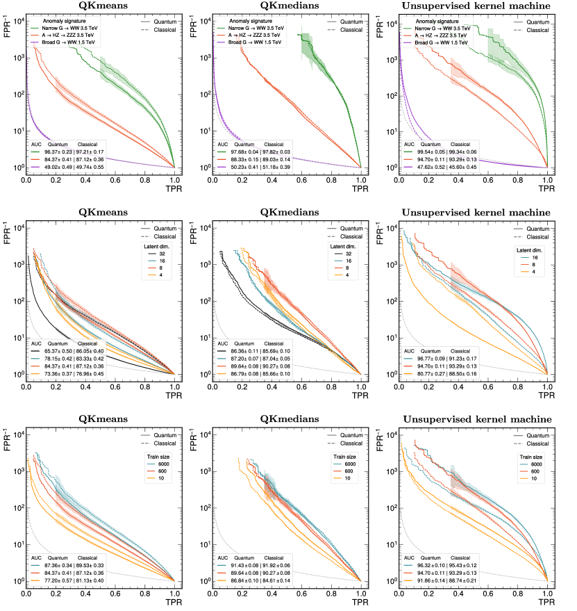
Figure 3: Performance evaluation results. Each subplot depicts the ROC curve calculation on test data for each model and each parameter of interest. Rows represent the model evaluation as a function of the parameters of interest: (top) new-physics anomalous signatures, (middle) latent space dimension, and (bottom) the number of training samples. Columns correspond to the different anomaly detection models. A 5-fold testing is performed to assess the statistical significance of the results and of the differences in performance, using a test dataset of $10^{5}$ samples where half of the samples are anomalies and half are SM events. The best-performing classical kernel model is the one equipped with the Radial Basis Function (RBF) kernel. The uncertainty bands represent one standard deviation and are drawn only for the TPR range of interest. For smaller values of TPR, the uncertainties increase due to low testing statistics and the bands are omitted for readability purposes.

Window of quantum advantage.

For the unsupervised kernel machine (third column of Fig. 3) we identify a consistent performance advantage. That is, there is a range in the investigated parameter space where we consistently obtain $\Delta_{\text{QC}}>1$. The performance advantage of the kernel-based quantum model is presented in more detail in Fig. 4, where it is quantified by $\Delta_{\text{QC}}$ and is related to intrinsic quantum properties of the circuit.

We show that if entanglement is not present in the quantum feature map the performance of the quantum model is worse or matches at best the classical performance. To demonstrate this, we construct two circuits NE₀ and NE₁, corresponding to removing all layers after the first set of encoding gates of the quantum circuit in Fig. 2a, and to removing only the CNOT gates between the two encoding layers, respectively. Furthermore, we show that an increase in the expressibility and entanglement of the circuit, accomplished by increasing the repetitions of the encoding ansatz, leads to the rise of the quantum algorithm performance up to a maximum at $L=4$ and a subsequent decrease for more expressive circuits. Conversely, too much entanglement, i.e., too many CNOT gates, causes a drop in $\Delta_{\mathrm{QC}}$ as presented by FE in Fig. 4, corresponding to a circuit with all-to-all entanglement layers instead of nearest-neighbors, and of fixed depth ($L=3$).

Additionally, if we fix the depth of the quantum circuit to three and investigate the performance of the quantum algorithm as a function of the number of qubits $\mathrm{n_{q}}$, we observe the following (see inner plot of Fig. 4). The quantum kernel machine performs worse in identifying anomalies for four qubits but is significantly better at the task for higher qubit numbers. We demonstrate a constant increase of the quantum model with the Hilbert space dimension, reaching a background rejection five times greater than that of its classical counterpart for 16 qubits. Explicit values of the background rejection are presented in Table 1a and Table 1b, for a fixed latent dimension and fixed training size, respectively.

Table 1: Background rejections. Comparing the background rejection $\varepsilon_{b}^{-1}(\varepsilon_{s})$ of the unsupervised quantum and classical kernel machines, for signal efficiencies $\varepsilon_{s}=0.6,0.8$. In Table (a) the background rejection is computed for a fixed latent dimension of 8 and the number of training samples is varied. In Table (b) the background rejection is calculated for a fixed training size of 600 and the dimensionality of the latent space is varied. Values are obtained using 5-fold testing of $N_{\mathrm{test}}=10^{5}$.

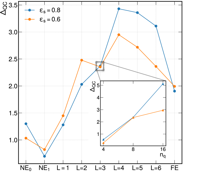
Figure 4: Relating the performance of the unsupervised quantum kernel machine to properties of the quantum circuit. The plot of the ratio $\Delta_{\mathrm{QC}}$, defined in Eq. 5, as a function of parameters of the data embedding quantum circuit presented in Fig. 2a. $\mathrm{L}$ denotes the number of repetitions of the ansatz, $\mathrm{NE_{0}}$ and $\mathrm{NE_{1}}$ represent cases where no entanglement is present in the circuit, and $\mathrm{FE}$ refers to all-to-all entanglement. For the case of three repetitions, $\Delta_{\mathrm{QC}}$ is also presented as a function of the number of qubits $\mathrm{n_{q}}$.

Quantum Hardware Calculations.

We implement the unsupervised kernel machine on a quantum computer, namely the ibm_toronto machine. The goal is to demonstrate the capability of the designed embedding circuit (cf. Fig. 2a) to run on current noisy near-term quantum devices. The size of the training and testing dataset is fixed at 100 and the number of qubits is eight. Further, the number of circuit evaluations needed during inference time to construct the quantum kernel matrix is $N_{\mathrm{train}}\cdot N_{\mathrm{test}}$. Hence, the number of testing samples is constrained not by the inherent limitations of the noisy near-term quantum device, but by the number of evaluations we can submit to the device via the IBMQ cloud in a reasonable amount of time. For more details on the quantum hardware implementation see App. D.

The results are presented in Table 2. We use the AUC to summarise the performance of the models, given the limited number of testing samples. The AUC is less prone to statistical fluctuation being the integral of the ROC curve, compared to the background rejection $\varepsilon_{b}^{-1}$, which corresponds to a point on the ROC curve. Consequently, we note that the values obtained on hardware, due to low testing statistics, are less accurate and should not be compared to the ones obtained by the more statistically robust computation using $10^{5}$ testing samples (cf. Fig. 3).

Additionally, the mean purity of the states $\braket{\mathrm{tr}\rho^{2}}\equiv\braket{k(x_{i},x_{i})}$, over the data points $x_{i}$, is measured on the quantum computer to ensure that throughout the computation the state has not decohered, i.e., lost its quantum nature due to noise and decoherence of the qubits. A fully mixed (decohered) state yields a purity of $1/2^{\mathrm{n_{q}}}$, where $\mathrm{n_{q}}$ is the number of qubits, resulting in approximately $0.39\times 10^{-2}$ for eight qubits. The hardware performance and the corresponding purities confirm that the designed quantum circuit for kernel-based anomaly detection, at least up to three repetitions, is indeed suitable for current quantum computers.

Kernel Machine Run	AUC	$\braket{\mathrm{tr}\rho^{2}}$
Hardware $L=1$	0.844	0.271(6)
Ideal $L=1$	0.999	1
Hardware $L=3$	0.997	0.15(2)
Ideal $L=3$	1.0	1
Classical	0.998	-

Table 2: Quantum hardware results. Comparing the performance of the unsupervised kernel machine in hardware and ideal simulation in terms of AUC, for one ($L=1$) and three ($L=3$) repetitions of the data encoding circuit. The mean purity $\braket{\mathrm{tr}\rho^{2}}$ is presented with its uncertainty in parenthesis at the corresponding decimal point.

V Conclusions

We presented a realistic study of QML models for anomaly detection in proton collisions at the LHC. The ability of the designed models to identify new-physics (BSM) events was thoroughly investigated using metrics of interest in HEP analyses. The proposed combination of an autoencoder that compresses raw HEP jet features to a tractable size, with quantum anomaly detection models proved to be a viable strategy for data-driven searches for new physics at the LHC.

In studies addressing classification tasks in HEP [20, 24, 23, 22, 21, 25, 26], so far, no significant difference in performance between quantum and classical ML models has been observed. In this work, to the best of our knowledge, we presented a first instance of the consistent performance advantage of QML models over classical models of similar complexity for an anomaly detection task in fundamental physics. This result, for the unsupervised quantum kernel machine, is statistically significant, is achieved using realistic datasets, and stretches beyond one-shot experiments or specific values of the considered parameter space. We demonstrated the role of intrinsically quantum properties of the developed data encoding circuit to achieve performance advantage and showed that the quantum model can reject up to five times more background events for a fixed signal efficiency (cf. Fig. 4).

The data encoding circuit for the quantum kernel is designed to have favorable properties, as discussed in Sec. III and IV. However, it is not explicitly biased to features characteristic to HEP data. Future studies need to investigate the construction of QML models that have an inductive bias towards the structure of HEP data to investigate for guarantees in terms of trainability and performance advantage. Recent works on QML share these insights in a more general context [9, 58, 59, 60, 61]. This way, we move towards answering the question of whether quantum models can be natural candidates for specific tasks in fundamental physics exploiting the data structure and its correlations in a more efficient way than their classical counterparts.

Additionally, we suggest that it is important to expose the quantum algorithms to features of minimal post-processing avoiding manual extraction of classical high-level features. In fact, the results of similar work in Ref. [62] reinforce this claim since the considered HEP dataset is described by high-level features and the dimensionality reduction is achieved through PCA. Along this direction, one possibility to provide the most direct and least processed access to the fundamental information of a physical system is to use quantum data, that is, to use quantum states as the input of QML models.

We anticipate that our results, along with the growing literature in QML for physics data and the parallel rapid improvement of available quantum hardware, can stimulate fruitful research at the intersection of hybrid quantum-classical algorithm design and fundamental physics data processing. Advancements along these lines can potentially lead to novel architectures and quantum-classical synergies, to performance advantages in well-defined sets of problems, and to the enhancement of our fundamental understanding of both fields.

Author Contributions

M.P. and K.A.W. prepared the dataset used in this work. K.A.W. designed and trained the classical autoencoder to compress the data, designed and trained the QK-means algorithm and trained its classical equivalent. V.B. designed the data encoding quantum circuit for the kernel machines, trained the corresponding quantum and classical models, related the observed performance advantage to the properties of the circuit, and implemented experiments on a quantum computer. E.P. designed and trained the QK-medians algorithm and trained its classical equivalent. All authors contributed to defining the research strategy, reviewing the results, and preparing this manuscript.

Data availability

The datasets used for this study are publicly available on Zenodo [63].

Code availability

The code developed for this paper is available publicly in the GitHub repository: https://github.com/vbelis/latent-ad-qml. All source code is also archived on Zenodo [64]. The Qiskit [65] framework is used to implement the quantum circuits of the unsupervised kernel machine and the QK-means algorithm, and Qibo [66] framework is used for QK-medians. For the expressibility and entanglement capability computation we used the software implementation in Ref. [67] (for details see App. B and C).

Appendix A Convolutional Autoencoder for dimensionality reduction

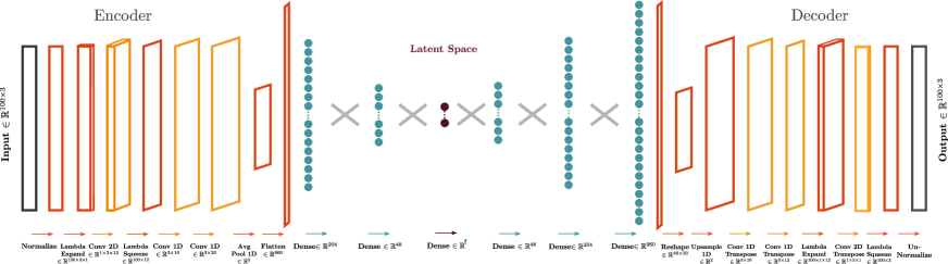
Figure 5: The Autoencoder architecture. The model reduces the dimensionality of the high energy physics dataset from 300 dimensions per jet to latent space dimension $\ell$. The generated latent space serves as the input to the anomaly detection algorithms.

To reduce the dimensionality of our low-level feature inputs, we developed an autoencoder, whose architecture is displayed in Fig. 5. The encoder consists of 1D and 2D convolutional layers, followed by pooling and dense layers. The decoder mirrors the architecture of the encoder. The bottleneck width defines the dimensionality of the latent space representation. Weights are He-uniform initialized and all layers feature Elu activations, except for a $\tanh$ activation right before the bottleneck, that constrains the latent space to a range $z\in(-1,1)$. The model is trained for 200 epochs with learning rate decay, minimizing the Chamfer-loss [68] defined as a pairwise reconstruction distance

$$L_{R}=\sum_{i\in\text{input}}\min_{j}((x^{(i)}-x^{(j)})^{2})+\sum_{j\in\text{output}}\min_{i}((x^{(j)}-x^{(i)})^{2}).$$ (6)

Inputs are standard-normalized at the entry to the encoder and outputs are de-normalized in the last layer of the decoder.

Appendix B Expressibility, entanglement capability, and data dependence

Background.

Expressibility and entanglement capability are measures, proposed in Ref. [41], to quantitatively describe properties of Parametrised Quantum Circuits (PQC). Expressibility measures the ability of a given PQC of $n$ qubits to explore the corresponding Hilbert space. A PQC of high expressibility is expected to generate, by sampling its parameters uniformly, (pure) quantum states that uniformly cover the Hilbert space. Specifically, expressibility is defined as the difference between the PQC-generated distribution of states and that of the ensemble of Haar-random states. The difference between the two distributions is quantified by the Kullback–Leibler divergence,

$$\mathcal{E}=D_{\mathrm{KL}}\left(P_{\mathrm{PQC}}(F;\theta)\,||\,P_{\mathrm{Haar}}(F)\right),$$ (7)

where $\theta$ represents the parameters of the circuit which are sampled from the uniform distribution over $[0,2\pi]$, $F$ is the fidelity $F=|\braket{\psi_{\theta}}{\psi_{\phi}}|^{2}$, between two PQC-generated states, $P_{\mathrm{PQC}}(F;\theta)$ is the probability density function of fidelities obtained by the states generated by the PQC, and

$$P_{\mathrm{Haar}}(F)=(N-1)(1-F)^{N-2},$$ (8)

is the probability distribution of fidelities of the Haar random states, where $N=2^{n}$ the dimension of the Hilbert space. By discretizing the distributions $P_{\mathrm{Haar}}$ and $P_{\mathrm{PQC}}$ using histograms, we can numerically calculate the expressibility of a quantum circuit. An expressive quantum circuit will obtain expressibility scores that approach zero as seen in Eq. 7.

The entanglement capability of a circuit is a measure of entanglement between the qubits based on the Meyer-Wallach measure $Q$ [41, 69]. We can estimate the measure numerically via sampling the parameters of the circuit uniformly in $[0,2\pi]$ and computing the mean,

$$\braket{Q}=\frac{1}{|\Theta|}\sum_{\theta\in\Theta}Q(\ket{\psi_{\theta}}),$$ (9)

where $\Theta$ is the set of parameters, correspondingly $|\Theta|$ the number of parameters, and $Q$ is the Meyer-Wallach measure. For more details and insights regarding these definitions refer to Ref. [41].

Data dependence.

The measures above are defined within the context of PQC-based algorithms, such as the variational quantum eigensolver. When dealing with data, as in this work, the notion of expressibility and entanglement capability needs to include the data distribution at hand. We extend the definitions in Eq. 7 and 9, similarly to recent work in Ref [61], to a data-dependent setting. Specifically, we sample the quantum circuit parameters from the distributions of the data features instead of the uniform distribution over $[0,2\pi]$. The input of the quantum models is the latent representation of the HEP datasets, described by the latent feature vector $z$ obtained by the encoder network (see App. A and Fig. 5). Depending on the data input, $z$ is distributed according to the QCD background distribution (SM) or the signal, anomalous (BSM) probability distribution. Hence, the expressibility measure can be written as,

$$\mathcal{E}=D_{\mathrm{KL}}\left(P_{U(z)}(F;z)\,||\,P_{\mathrm{Haar}}(F)\right),$$ (10)

where $P_{U(z)}(F;z)$ represents the fidelity distribution of the states generated by the data encoding ansatz $U$ (see Fig. 2) when the features are sampled from an arbitrary probability density function $\mathcal{P}(z)$. Similarly, for the entanglement capability we can calculate $\braket{Q}$ in Eq. 9 by sampling from $\mathcal{P}(z)$.

We compute the expressibility and entanglement capability of the designed circuit, for the case of eight qubits, as a function of the architecture variations presented in Sec. IV and in Fig. 4. For this computation, we use the software implementation in Ref. [67]. The results are presented in Fig. 6a and  6b, where the three different curves correspond to three different choices of $\mathcal{P}(z)$: sampling from the uniform distribution in $[0,2\pi]$, the QCD background, and the signal distribution of the scalar boson BSM scenario, respectively. The number of samples is $6\times 10^{5}$ for each data-dependent computation in Fig. 6. We verify that by increasing the depth of the proposed data encoding circuit its expressibility and entanglement capability are increased for all assessed data distributions. These results combined with Fig. 4 demonstrate a correlation between the performance of the unsupervised kernel machine on HEP data and quantum properties of the designed feature map.

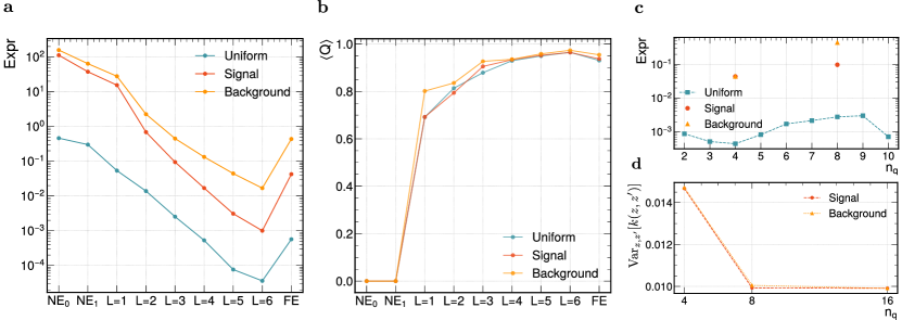
Figure 6: Characterization metrics of the data encoding circuit. The metrics are calculated via sampling the circuit parameters from three different distributions as depicted in the legends: the uniform distribution in $[0,2\pi]$, the QCD background data distribution, and the signal (anomaly) scalar boson data distribution. (a) The expressibility (Expr) as a function of the different circuit architectures. (b) The entanglement capability of the data encoding circuit ($\langle\mathrm{Q}\rangle$) as a function of the different circuit architectures. (c) The expressibility of the data encoding circuit as a function of the number of qubits ($\mathrm{n_{q}}$). (d) The variance of the kernel, $\mathrm{Var}_{z,z^{\prime}}k(z,z^{\prime})$, where $k(z,z^{\prime})$ is the kernel defined in Eq. 1 and $z$ is the data feature vector sampled from the signal or background distributions corresponding to the data encoding circuit as a function of the number of qubits.

Appendix C Trainability of the kernel machine and exponential concentration

One of the advantages of kernel-based (Q)ML is the theoretical guarantee of a global extremum of the objective function that can be found through convex optimisation  [70]. Recently, in Ref. [61], the trainability of quantum kernel methods in QML is studied and challenged within the scope of exponential concentration, i.e. the case where all elements of the kernel matrix converge exponentially fast to a single value and render the model ineffective. Therein, different sources of exponential concentration are identified, such as the expressibility of the circuit and the use of global measurements.

In our study, we do not observe such limitations based on the performance assessment of the unsupervised quantum kernel machines (cf. Sec. IV). Here, we investigate further the scaling of the expressibility of the data encoding circuit and the variance of the corresponding quantum kernel with the number of qubits. These computations provide insights on the trainability of our models beyond the tested datasets. In Fig. 6c and Fig. 6d we present the expressibility and variance of the kernel, respectively. The dimensionality of the available HEP datasets used in this work is restricted to $\mathrm{n_{q}}=4,8,16$, where $\mathrm{n_{q}}$ is the number of qubits. The available $6\times 10^{5}$ data samples were sufficient to evaluate accurately the expressibility for four and eight qubits, but not 16. Hence, only results for four and eight qubits are presented in Fig. 6c when sampling the circuit parameters from the data distributions.

Overall, an almost constant dependence between the expressibility and the number of qubits is observed in Fig. 6c, contrary to one of the assumptions of Theorem 1 in Ref. [61], where the expressibility of the data encoding circuit be exponentially close to a 2-design. That is, $\mathcal{E}\in\mathcal{O}(1/b^{n})$, where $b>1$ and $n$ is the number of qubits. In the case of kernel variance scaling, no exponential decay seems to be manifest. Thus, our calculations suggest that the proposed unsupervised kernel machine does not suffer from exponential concentration due to expressibility or global measurements. Nevertheless, our numerical experiments are restricted to the presented number of qubits. HEP datasets can be generated specifically with the purpose of assessing quantum kernel properties more thoroughly, which can be the subject of future studies.

Appendix D Implementing the unsupervised kernel machine

Training set-up.

We present the optimisation task of the unsupervised kernel machine in its primal form adopting the notation from Ref. [51] for completeness. Given a set of training data $x_{1},x_{2},\dots,x_{\ell}\in\mathcal{X}$, where $\mathcal{X}$ is an arbitrary vector space, $\ell$ is the number of training data points, and $x_{i}$ represent the feature vectors of the data, one can write the objective function of the model and its corresponding constraints as

$$\min_{w\in\mathcal{F},\,\xi\in\mathbb{R}^{\ell},\,\rho\in\mathbb{R}}\quad\frac{1}{2}||w||^{2}+\frac{1}{\nu\ell}\sum_{i}\xi_{i}-\rho$$ (11)

$$\mathrm{subject\;to}\quad w\cdot\Phi(x_{i})\geq\rho-\xi_{i},\,\xi_{i}\geq 0,\;\forall i,$$ (12)

where $\Phi:\mathcal{X}\mapsto\mathcal{F}$ is the feature map, which is used to define the kernel $k(x_{i},x_{j})=\Phi(x_{i})\circ\Phi(x_{j})$, $\mathcal{F}$ is the feature space, $w$ are the trainable weights of the model, $\xi_{i}$ are the slack variables, $\rho$ is the distance of the hyperplane from the origin of the feature space, and $\nu\in(0,1)$ is a hyperparameter. Training the kernel machines corresponds to solving the optimisation problem above with respect to $w$ and $\rho$. It can be shown that $\nu$ is an upper bound on the fraction of outliers, or anomalies following the nomenclature of this manuscript, in the training dataset [51].

An optimal $\nu$ cannot be identified globally for every possible signal distribution, i.e., BSM scenario, in the unsupervised anomaly detection context. On the contrary, in a supervised learning setting where the specific signal and background are known by construction, one can hyperoptimise the ML algorithm using model selection techniques. Choosing a value of $\nu$ based on hyperoptimisation with respect to a specific BSM dataset can lead to biasing the model towards this particular anomaly distribution. Although this can increase the performance of the model on the chosen BSM signature, the sensitivity of the anomaly detection strategy can be diminished for other new-physics scenarios. Hence, such a procedure can lead to overall reduced performance of the anomaly detection model and is not consistent with the initial motivation behind model-independent searches of new physics at the LHC experiments as presented in Sec. I.

For our study, we choose $\nu=0.01$ and keep it fixed for all investigated models and BSM datasets. Therefore, we assume that the model should, falsely, flag at most $1\%$ of the QCD background samples used for training. Furthermore, given the small training sizes used for the quantum models, e.g. 600, smaller values of $\nu$ would lead to a none-integer upper bound on the number of outliers causing the optimisation problem in Eq. 11 and 12 to be ill-defined.

Quantum hardware implementation.

The unsupervised quantum kernel machine has been implemented for both the quantum hardware and simulation computations using qiskit [65]. The data encoding circuit (see Fig. 2) used to construct the feature map of the quantum kernel needs to be transpiled to the gates that are native to the hardware device: $R_{z},\sqrt{X},X,$ and $CX$(CNOT). Due to the presence of noise in quantum hardware, the sampled kernel matrix need not be positive semi-definite (PSD). For this reason, the matrix that we retrieve from the hardware is transformed to the closest PSD matrix to ensure that the convex optimization task of the algorithm is well-defined. Furthermore, the qubits of the algorithm need to be mapped to the physical qubits of the hardware, which for the ibm_toronto machine follow the topology depicted in Fig. 7.

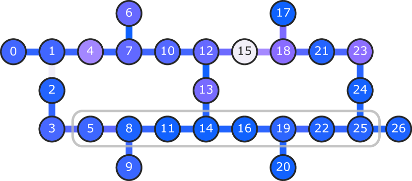
Figure 7: Topology of physical qubits. The layout of the physical qubits on the ibm_toronto machine. The connections between nodes represent the possibility of executing 2-qubit gates between neighboring qubits. The selected eight qubits, circled in grey, represent the ones used to run the quantum kernel machine. Different noise levels are color-coded, the lighter color representing higher noise levels, for single qubit and 2-qubit gates on the nodes and connections, respectively.

We execute our models using the following physical qubits: $[5,8,11,14,16,19,22,25]$, corresponding to the indexing in Fig. 7. This choice is based on the calibration data provided at the time of submitting the run, taking into account the estimated gate and measurement noise. Simultaneously, we ensure nearest-neighbors connections between the physical qubits to not introduce unnecessary SWAP gates which increase significantly the depth of the transpiled circuit.

References

- Rebentrost et al. [2014] P. Rebentrost et al., Quantum support vector machine for big data classification, Physical review letters 113, 130503 (2014).
- Biamonte et al. [2017] J. Biamonte et al., Quantum machine learning, Nature 549, 195 (2017).
- Schuld and Petruccione [2018] M. Schuld and F. Petruccione, Supervised Learning with Quantum Computers (Springer International Publishing, 2018).
- Schuld and Killoran [2019] M. Schuld and N. Killoran, Quantum machine learning in feature hilbert spaces, Physical Review Letters 122, 10.1103/physrevlett.122.040504 (2019).
- M. Schuld et al. [2020] M. M. Schuld et al., Circuit-centric quantum classifiers, Phys. Rev. A 101, 032308 (2020).
- Havlíček et al. [2019] V. Havlíček, A. Córcoles, K. Temme, et al., Supervised learning with quantum-enhanced feature spaces, Nature 567, 209 (2019).
- Lloyd et al. [2020] S. Lloyd et al., Quantum embeddings for machine learning 10.48550/arXiv.2001.03622 (2020), arXiv:2001.03622 [quant-ph].
- Abbas et al. [2021] A. Abbas et al., The power of quantum neural networks, Nature Computational Science 1, 403 (2021).
- Huang et al. [2021] H. Huang et al., Power of data in quantum machine learning, Nature Communications 12, 2631 (2021).
- Liu et al. [2021] Y. Liu et al., A rigorous and robust quantum speed-up in supervised machine learning, Nature Physics 17, 1013 (2021).
- Huang et al. [2022] H. Huang et al., Quantum advantage in learning from experiments, Science 376, 1182 (2022).
- Caro et al. [2022] M. Caro et al., Generalization in quantum machine learning from few training data, Nature Communications 13, 4919 (2022), number: 1 Publisher: Nature Publishing Group.
- Cong et al. [2019] I. Cong et al., Quantum convolutional neural networks, Nature Physics 15, 1273 (2019).
- Mott et al. [2017] A. Mott et al., Solving a Higgs optimization problem with quantum annealing for machine learning, Nature 550, 375 (2017).
- Tüysüz et al. [2020] C. Tüysüz et al., Particle track reconstruction with quantum algorithms, EPJ Web of Conferences 245, 09013 (2020).
- Tüysüz et al. [2021] C. Tüysüz et al., Hybrid quantum classical graph neural networks for particle track reconstruction, Quantum Machine Intelligence 3, 29 (2021).
- Magano et al. [2022] D. Magano et al., Quantum speedup for track reconstruction in particle accelerators, Physical Review D 105, 076012 (2022), publisher: American Physical Society.
- de Lejarza et al. [2022] J. M. de Lejarza et al., Quantum clustering and jet reconstruction at the lhc, Phys. Rev. D 106, 036021 (2022).
- Duckett et al. [2022] P. Duckett et al., Reconstructing charged particle track segments with a quantum-enhanced support vector machine (2022), arXiv:2212.07279 .
- Guan et al. [2021] W. Guan et al., Quantum machine learning in high energy physics, 2, 011003 (2021).
- Wu et al. [2021] S. Wu et al., Application of quantum machine learning using the quantum kernel algorithm on high energy physics analysis at the lhc, Phys. Rev. Research 3, 033221 (2021).
- Terashi et al. [2021] K. Terashi et al., Event Classification with Quantum Machine Learning in High-Energy Physics, Comput. Softw. Big Sci. 5, 2 (2021), arXiv:2002.09935 [physics.comp-ph] .
- Blance and Spannowsky [2020] A. Blance and M. Spannowsky, Quantum Machine Learning for Particle Physics using a Variational Quantum Classifier 10.1007/JHEP02(2021)212 (2020), arXiv:2010.07335 [hep-ph] .
- Belis et al. [2021] V. Belis et al., Higgs analysis with quantum classifiers, EPJ Web Conf. 251, 03070 (2021).
- Alvi et al. [2022] S. Alvi et al., Quantum Anomaly Detection for Collider Physics (2022), arXiv:2206.08391 [hep-ph] .
- Ngairangbam et al. [2022] V. Ngairangbam et al., Anomaly detection in high-energy physics using a quantum autoencoder, Phys. Rev. D 105, 095004 (2022).
- Aad et al. [2012] G. Aad et al. (ATLAS), Observation of a new particle in the search for the Standard Model Higgs boson with the ATLAS detector at the LHC, Phys. Lett. B 716, 1 (2012), arXiv:1207.7214 [hep-ex] .
- The ATLAS Collaboration [2022] The ATLAS Collaboration, A detailed map of higgs boson interactions by the atlas experiment ten years after the discovery, Nature 607, 52–59 (2022).
- Chatrchyan et al. [2012] S. Chatrchyan et al. (CMS), Observation of a New Boson at a Mass of 125 GeV with the CMS Experiment at the LHC, Phys. Lett. B 716, 30 (2012), arXiv:1207.7235 [hep-ex] .
- The CMS Collaboration [2022] The CMS Collaboration, A portrait of the higgs boson by the cms experiment ten years after the discovery, Nature 607, 60–68 (2022).
- Heimel et al. [2019] T. Heimel et al., QCD or What?, SciPost Phys. 6, 030 (2019), arXiv:1808.08979 [hep-ph] .
- Farina et al. [2020] M. Farina et al., Searching for New Physics with Deep Autoencoders, Phys. Rev. D 101, 075021 (2020), arXiv:1808.08992 [hep-ph] .
- Kasieczka et al. [2021] G. Kasieczka et al., The LHC Olympics 2020 a community challenge for anomaly detection in high energy physics, Rept. Prog. Phys. 84, 124201 (2021), arXiv:2101.08320 [hep-ph] .
- Aarrestad et al. [2022] T. Aarrestad et al., The Dark Machines Anomaly Score Challenge: Benchmark Data and Model Independent Event Classification for the Large Hadron Collider, SciPost Phys. 12, 043 (2022).
- Cerri et al. [2019] O. Cerri et al., Variational Autoencoders for New Physics Mining at the Large Hadron Collider, JHEP 05, 036, arXiv:1811.10276 [hep-ex] .
- Knapp et al. [2021] O. Knapp et al., Adversarially Learned Anomaly Detection on CMS Open Data: re-discovering the top quark, Eur. Phys. J. Plus 136, 236 (2021), arXiv:2005.01598 [hep-ex] .
- Aad et al. [2020] G. Aad et al. (ATLAS), Dijet resonance search with weak supervision using TeV collisions in the ATLAS detector, Phys. Rev. Lett. 125, 131801 (2020), arXiv:2005.02983 [hep-ex] .
- ATL [2022] Anomaly detection search for new resonances decaying into a Higgs boson and a generic new particle in hadronic final states using = 13 TeV collisions with the ATLAS detector, (2022).
- Lloyd et al. [2013] S. Lloyd et al., Quantum algorithms for supervised and unsupervised machine learning (2013), arXiv:1307.0411 [quant-ph] .
- Gao et al. [2022] X. Gao et al., Enhancing generative models via quantum correlations, Physical Review X 12, 021037 (2022).
- Sim et al. [2019] S. Sim et al., Expressibility and entangling capability of parameterized quantum circuits for hybrid quantum-classical algorithms, Advanced Quantum Technologies 2, 1900070 (2019), arXiv:1905.10876 [quant-ph].
- Sjöstrand et al. [2015] T. Sjöstrand et al., An Introduction to PYTHIA 8.2, Comput. Phys. Commun. 191, 159 (2015), arXiv:1410.3012 [hep-ph] .
- Randall and Sundrum [1999] L. Randall and R. Sundrum, A Large mass hierarchy from a small extra dimension, Phys. Rev. Lett. 83, 3370 (1999), arXiv:hep-ph/9905221 .
- Bijnens et al. [2001] J. Bijnens et al., QCD signatures of narrow graviton resonances in hadron colliders, Phys. Lett. B 503, 341 (2001), arXiv:hep-ph/0101316 .
- de Favereau et al. [2014] J. de Favereau et al. (DELPHES 3), DELPHES 3, A modular framework for fast simulation of a generic collider experiment, JHEP 02, 057, arXiv:1307.6346 [hep-ex] .
- Cacciari et al. [2008] M. Cacciari et al., The anti- jet clustering algorithm, JHEP 04, 063, arXiv:0802.1189 [hep-ph] .
- Cacciari et al. [2012] M. Cacciari et al., FastJet User Manual, Eur. Phys. J. C 72, 1896 (2012), arXiv:1111.6097 [hep-ph] .
- Preskill [2018] J. Preskill, Quantum computing in the NISQ era and beyond, Quantum 2, 79 (2018).
- [49] K. A. Woźniak et al., Classical anomaly detection study, manuscript in preparation .
- Boser et al. [1992] B. E. Boser et al., A training algorithm for optimal margin classifiers, Proceedings of the fifth annual workshop on Computational learning theory (1992).
- Schölkopf et al. [1999] B. Schölkopf, R. C. Williamson, A. Smola, J. Shawe-Taylor, and J. Platt, Support vector method for novelty detection, in Advances in Neural Information Processing Systems, Vol. 12, edited by S. Solla et al. (MIT Press, 1999).
- LaRose and Coyle [2020] R. LaRose and B. Coyle, Robust data encodings for quantum classifiers, Phys. Rev. A 102, 032420 (2020).
- Khan et al. [2019] S. Khan et al., K-means clustering on noisy intermediate scale quantum computers (2019).
- Durr and Hoyer [1999] C. Durr and P. Hoyer, A quantum algorithm for finding the minimum (1999), arXiv:quant-ph/9607014 [quant-ph] .
- Boyer et al. [1998] M. Boyer et al., Tight bounds on quantum searching, Fortschritte der Physik 46, 493–505 (1998).
- Grover [1996] L. K. Grover, A fast quantum mechanical algorithm for database search (1996), arXiv:quant-ph/9605043 [quant-ph] .
- Vardi and Zhang [2000] Y. Vardi and C. Zhang, The multivariate -median and associated data depth, Proceedings of the National Academy of Sciences 97, 1423 (2000), https://www.pnas.org/doi/pdf/10.1073/pnas.97.4.1423 .
- Kübler et al. [2021] J. Kübler et al., The inductive bias of quantum kernels, in Advances in Neural Information Processing Systems, Vol. 34, edited by M. Ranzato, A. Beygelzimer, Y. Dauphin, P. S. Liang, and J. W. Vaughan (Curran Associates, Inc., 2021) p. 12661–12673.
- Pesah et al. [2021] A. Pesah et al., Absence of barren plateaus in quantum convolutional neural networks, Physical Review X 11, 041011 (2021).
- Meyer et al. [2022] J. Meyer et al., Exploiting symmetry in variational quantum machine learning 10.48550/arXiv.2205.06217 (2022), arXiv:2205.06217 [quant-ph].
- Thanasilp et al. [2022] S. Thanasilp et al., Exponential concentration and untrainability in quantum kernel methods 10.48550/arXiv.2208.11060 (2022), arXiv:2208.11060 [quant-ph, stat].
- Schuhmacher et al. [2023] J. Schuhmacher et al., Unravelling physics beyond the standard model with classical and quantum anomaly detection (2023), arXiv:2301.10787 .
- Pierini and Wozniak [2023] M. Pierini and K. A. Wozniak, Dataset for Quantum anomaly detection in the latent space of proton collision events at the LHC, 10.5281/zenodo.7673769 (2023).
- Belis et al. [2023] V. Belis, E. Puljak, and K. A. Wozniak, vbelis/latent-ad-qml: v1.0.4 10.5281/zenodo.7696203 (2023).
- Abby-Mitchell et al. [2021] Abby-Mitchell et al., Qiskit: An open-source framework for quantum computing (2021).
- Efthymiou et al. [2021] S. Efthymiou et al., Qibo: a framework for quantum simulation with hardware acceleration, Quantum Science and Technology 7, 015018 (2021).
- Muser and Belis [2023] T. Muser and V. Belis, triple_e: Characterisation metrics package for parametrised quantum circuits 10.5281/zenodo.7643539 (2023).
- Fan et al. [2017] H. Fan et al., A point set generation network for 3d object reconstruction from a single image, in 2017 IEEE Conference on Computer Vision and Pattern Recognition (CVPR) (2017) p. 2463, arXiv:1612.00603 [cs.CV] .
- Meyer and Wallach [2002] D. A. Meyer and N. R. Wallach, Global entanglement in multiparticle systems, Journal of Mathematical Physics 43, 4273 (2002).
- Schuld [2021] M. Schuld, Supervised quantum machine learning models are kernel methods (2021), arXiv:hep-ph/9905221 .