$T-$linear resistivity from magneto-elastic scattering: application to PdCrO₂

Abstract

An electronic solid with itinerant carriers and localized magnetic moments represents a paradigmatic strongly correlated system. The electrical transport properties associated with the itinerant carriers, as they scatter off these local moments, has been scrutinized across a number of materials. Here we analyze the transport characteristics associated with ultra-clean PdCrO₂ — a quasi two-dimensional material consisting of alternating layers of itinerant Pd-electrons and Mott-insulating CrO₂ layers — which shows a pronounced regime of $T-$linear resistivity over a wide-range of intermediate temperatures. By contrasting these observations to the transport properties in a closely related material PdCoO₂, where the CoO₂ layers are band-insulators, we can rule out the traditional electron-phonon interactions as being responsible for this interesting regime. We propose a previously ignored electron-magnetoelastic interaction between the Pd-electrons, the Cr local-moments and an out-of-plane phonon as the main scattering mechanism that leads to the significant enhancement of resistivity and a $T-$linear regime in PdCrO₂ at temperatures far in excess of the magnetic ordering temperature. We suggest a number of future experiments to confirm this picture in PdCrO₂, as well as other layered metallic/Mott-insulating materials.

Introduction.- Recent years have witnessed a resurgence of interest in the microscopic origin of an electrical resistivity that scales linearly with temperature [1, 2] and exhibiting a Planckian scattering rate, $\Gamma=Ck_{B}T/\hbar$, where $C\sim O(1)$ coefficient [3, 4, 5, 6, 7]. In conventional (simple) metals at room temperature, this phenomenology is readily understood as a consequence of electrons scattering off thermally excited phonons in their equipartition regime [8]. On the other hand, numerous “correlated” materials belonging to the cuprate [9, 10, 6, 7], pnictide [11, 12], ruthenates [13, 14, 15, 16, 17], rare-earth [18] and moiré bilayers [5, 19] display Planckian scattering down to low temperatures, likely driven by purely electronic interactions and where a priori it is unclear if phonons play an essential role [3, 20, 21, 22]. It is challenging to disentangle the role of electron-electron and electron-phonon interactions on scattering lifetimes. It is quite natural to ask if materials with a nearly identical phonon spectrum and distinct electronic spectra can lead to a distinct temperature dependence of their respective resistivities.

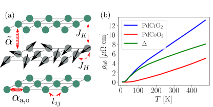
Figure 1: (a) The structural motif in PdCrO₂, composed of alternating layers of triangular lattices of conducting Pd planes (green) and Mott insulating CrO₂ planes (grey). The different coupling constants denoted in the figure are as defined in Eq. (1). (b) The in-plane resistivities of PdCrO₂ and PdCoO₂ taken from Ref. [23] along with their difference $\Delta\rho\equiv\rho_{ab}^{\rm PdCrO_{2}}-\rho_{ab}^{\rm PdCoO_{2}}>0$.

An experimental puzzle.- The goal of this letter is to resolve a conundrum inspired by electrical transport measurements in two isostructural quasi two-dimensional compounds with distinct electronic structures: PdCoO₂ and PdCrO₂. Their structural motif consists of alternately stacked layers of highly conducting Pd and insulating CoO₂/CrO₂ in a triangular lattice arrangement [24, 25, 26, 27, 28]; see Fig. 1(a). The phonon spectra for the two compounds are nearly identical; some of the differences arise from the distinct ionic masses [29, 30, 27, 28], and recent analysis has also revealed that the unit cell of PdCrO₂ is slightly enlarged due to the presence of magnetic moments [31]. On the other hand, their electronic spectra are different since the CrO₂ layers are Mott-insulating with the local-moments interacting via antiferromagnetic (AFM) exchange interactions [25, 32], while the CoO₂ layers are non-magnetic [24, 26, 33]. The photoemission spectrum of PdCrO₂ contains prominent features, absent in PdCoO₂ [34, 35, 36, 28], that can be understood from an effective inter-layer Kondo lattice model [28]. The in-plane resistivities for the two compounds [23] are shown in Fig. 1(b), respectively. The salient features are as follows: (i) The magnitude of the resistivity for both compounds is small, suggesting that they are “good” metals with a long mean-free path. (ii) PdCrO₂ is considerably more resistive than PdCoO₂ over a wide range of temperatures. (iii) PdCrO₂ displays a prominent $T-$linear scaling of the resistivity above $T\gtrsim 150$K (far above $T_{\rm N}\approx 37.5$K, the Néel temperature for $120^{\circ}-$antiferromagnetism) [25, 37, 32, 38], and with a slope that is greater than the average slope of $\rho_{ab}(T)$ in PdCoO₂ in the same temperature range [39].

The central puzzle that we address in this Letter concerns the microscopic origin of the excess $T-$linear resistivity in PdCrO₂ relative to isostructural PdCoO₂ ($\Delta\rho\equiv\rho_{ab}^{\rm PdCrO_{2}}-\rho_{ab}^{\rm PdCoO_{2}}>0$), going beyond the conventional electron-phonon scattering mechanism, and in a temperature regime where the long-range magnetic order is lost. Given the contrast between PdCrO₂ and PdCoO₂, it is plausible that the fluctuations of the Cr-local moments play a crucial role on the electronic transport lifetimes even at the relatively high temperatures of interest (i.e. for $T\gtrsim T_{N}$). However, recent work [40] has demonstrated that electrons scattering off the fluctuations of a “cooperative” paramagnet [41, 42, 43, 44, 45, 46, 47, 48] can not account for a $T-$linear resistivity; instead the resistivity saturates to a temperature-independent value for $T\gg T_{N}$. Starting with a microscopic model, we will now demonstrate that the resolution to the conundrum lies in a previously ignored and non-trivial interaction term between the Pd-electrons, the Cr-spins, and phonons, as encoded in an electron-magneto-elastic (EME) coupling. Although specifically motivated by PdCrO₂, our theory has relevance beyond this single material. There are a number of exciting new material platforms that have come to the forefront in recent years that consist of stacks of metallic and Mott insulating layers [49, 50, 51, 52, 53, 54, 55, 56, 57]. In what follows, we develop a general framework to address electrical transport in such layered material platforms, and our conclusions can be used to disentangle the various sources of interaction between electrons, local-moments and phonon degrees of freedom.

Model.- Consider a quasi two-dimensional (2D) layered model defined on a triangular lattice, where the electronic and local-moment degrees of freedom reside on alternating layers. The effective 2D Hamiltonian is given by (see [39] for a microscopic derivation of $H_{\rm{EME}}$),

$$H = H_{\rm el}+H_{\rm S}+H_{\rm K}+H_{\rm ph}+H_{\rm el-ph}+H_{\rm EME},$$

$$H_{\text{el}} = \sum_{\bm{k},\alpha}(\varepsilon_{\bm{k}}-\mu)p_{\bm{k}\alpha}^{\dagger}p^{\phantom{\dagger}}_{\bm{k}\alpha},$$ (1b)

$$H_{\text{S}} = J_{\text{H}}\sum_{\left\langle i,j\right\rangle}\bm{S}_{i}\cdot\bm{S}_{j},$$ (1c)

$$H_{\text{K}} = J_{\text{K}}\sum_{i}p^{\dagger}_{i\alpha}(\bm{S}_{i}\cdot\bm{\sigma}_{\alpha\beta})p^{\phantom{\dagger}}_{i\beta},$$ (1d)

$$H_{\text{ph}} = \sum_{\ell=I_{\rm a},I_{\rm o},O}\sum_{\bm{q}}\left(\frac{|\pi^{(\ell)}_{\bm{q}}|^{2}}{2M}+\frac{M\omega_{\ell,\bm{q}}^{2}}{2}|\varphi^{(\ell)}_{\bm{q}}|^{2}\right),$$ (1e)

$$H_{\rm{el-ph}} = \sum_{i,\sigma}\bigg{(}\alpha_{\rm a}\nabla\varphi^{(I_{\rm a})}_{i}p_{{i}\sigma}^{\dagger}p^{\phantom{\dagger}}_{{i}\sigma}+\alpha_{\rm o}\varphi^{(I_{\rm o})}_{i}p_{{i}\sigma}^{\dagger}p^{\phantom{\dagger}}_{{i}\sigma}\bigg{)},$$ (1f)

$$H_{\text{EME}} = \widetilde{\alpha}\sum_{i}\varphi^{(O)}_{i}p^{\dagger}_{i\alpha}(\bm{S}_{i}\cdot\bm{\sigma}_{\alpha\beta})p^{\phantom{\dagger}}_{i\beta}.$$ (1g)

Here $p^{\dagger}_{\bm{k}\sigma},\leavevmode\nobreak\ p^{\phantom{\dagger}}_{\bm{k}\sigma}$ denote the Pd-electron creation and annihilation operators with momentum $\bm{k}$ and spin $\sigma=\pm 1/2$. The electronic dispersion is given by $\varepsilon_{\bm{k}}$ and $\mu$ is the chemical potential; experiments in PdCrO₂ indicate the Pd-electronic structure is well captured using first and second-neighbor hoppings and the conduction band, dominantly of Pd character, is very close to half-filling [28, 23]. The local-moments, $\bm{S}_{i}$, interact mutually via nearest-neighbor antiferromagnetic Heisenberg exchange ($J_{\rm H}>0$), and with the Pd-electron spin-density via a Kondo exchange ($J_{\rm K}>0$), respectively. The Cr-electrons form $S=\frac{3}{2}$ local-moments [28]. Finally, we include three phonon fields, $\varphi^{(\ell)}$ with $\ell=I_{\rm{a}},I_{\rm{o}},\leavevmode\nobreak\ O$, corresponding to in-plane acoustic ($I_{\rm a}$), in-plane optical ($I_{\rm o}$) and out-of-plane ($O$) lattice vibrations, respectively. We set the mass, $M$, to be equal for these modes for simplicity. The in-plane modes $I_{\rm a,o}$ couple to the $p$-electron density with strengths $\alpha_{\rm a,o}$, respectively, while the out-of-plane mode, $O$, couples to the “inter-layer” Kondo interaction with EME strength, $\widetilde{\alpha}$. We set the lattice constant $a=1$, unless stated otherwise. Importantly, we include couplings to both in-plane acoustic and optical modes to account for the full $T$-dependence of $\rho_{ab}$ in the absence of magnetism (i.e. in PdCoO₂) [29]. Henceforth, we neglect the weak momentum dependence and the form-factors associated with the different interaction terms in the quasi two-dimensional setting to simplify our discussion [28]. We will restore these additional complexities when considering out-of-plane transport for reasons to be made clear below.

Let us begin by considering the simpler case where the optical modes are Einstein-phonons, with ${\omega}_{I_{\rm o},\bm{q}}=\omega_{0}$ and $\omega_{O,\bm{q}}=\widetilde{\omega}_{0}$, while for the acoustic mode ${\omega}_{I_{\rm a},\bm{q}}=cq$, with a corresponding Debye frequency $\omega_{D}$. The experimental regime of interest corresponds to $\{\widetilde{\omega}_{0},J_{\rm{H}}\}\lesssim T\ll\varepsilon_{F}$, where $\varepsilon_{F}$ is the Fermi energy for the Pd-electrons. Moreover, we shall consider the limit where $J_{\rm{H}}\gg\{\widetilde{\alpha}\sqrt{\hbar/M\widetilde{\omega}_{0}},\leavevmode\nobreak\ J_{\rm{K}}\}$ and thereby ignore the feedback of both electrons and phonons on the properties of the local-moments. In recent work [40], some of us analyzed the properties of a subset of the terms, ($H_{\textnormal{el}}+H_{\textnormal{S}}+H_{\textnormal{K}}$), in Eq. (1) at leading order in a small $J_{\rm{K}}$ by approximating the local-moments as $O(3)$ vectors, but capturing their complex precessional dynamics using the Landau-Lifshitz equations [41, 42, 43, 44, 45, 46, 47, 48]. While this leads to an interesting frequency dependence and momentum-dependent crossovers in the electronic self-energy, the temperature dependence can be understood entirely based on a high-temperature expansion with uncorrelated local-moments. The present manuscript will treat the local-moments on the same footing, but include the additional interaction effects due to ($H_{\rm{ph}}+H_{\rm{el-ph}}+H_{\rm{EME}}$).

Results for intermediate-scale transport.- We will analyze electrical transport for the model defined above within the framework of traditional Landau-Boltzmann paradigm [8]. This is justified based on the magnitude of the resistivity being much smaller than the characteristic scale of $ha_{B}/e^{2}$ ($a_{B}\equiv$Bohr radius) and $k_{F}\ell_{\rm mfp}\gg 1$ over the entire temperature range of interest ($\ell_{\rm mfp}$ being the mean free path) [23]. Moreover, there is direct experimental evidence for the value of the dimensionless Kondo-coupling being small, based on recent photoemission experiments [28].

Considering the full $H$, we have multiple sources of scattering for the electrons. Within Boltzmann theory, the total transport scattering rate satisfies Matthiessen’s rule [8]:

$$\frac{1}{\tau_{\rm tr}}=\frac{1}{\tau_{\rm{el-ph}}}+\frac{1}{\tau_{\rm K}}+\frac{1}{\tau_{\rm EME}},$$ (2)

and the in-plane resistivity is given by $\rho_{ab}=m/(ne^{2}\tau_{\rm tr})$, where $m$ is the effective mass and $n$ is the electron density [39]. Experiments with controlled amounts of irradiation shift the overall resistivity curves by a constant (and relatedly, the residual resistivity), without affecting the slope in the $T-$linear regime [31]. We start by describing the electron-phonon contribution, $1/\tau_{\rm{el-ph}}\equiv 1/\tau_{\rm{el-ph},a}+1/\tau_{\rm{el-ph},o}$. Previous works have obtained $1/\tau_{\rm{el-ph}}$ for PdCoO₂, and highlighted the importance of a high-frequency optical mode (which is not entirely in the equipartition regime at $T\lesssim\omega_{0}$) for the observed superlinear-scaling of $\rho_{ab}(T)$ [29, 58]. We have fully reproduced these results for PdCoO₂ based on the same procedure [39] within our 2D model of the Fermi surface; see Fig. 2. In PdCrO₂, the scattering of electrons off the local-moments due to the bare Kondo interaction, $1/\tau_{\rm K}$, can lead to a sub-linear $T$-dependent contribution to $\rho_{ab}$ at temperatures $T\gtrsim J_{\rm H}$, before saturating to the $T$-independent value [40] (see $\rho_{\rm K}=m/(ne^{2}\tau_{\rm K})$ in the inset of Fig. 2).

We now turn to the important role of the EME term in PdCrO₂. For $\widetilde{\omega}_{0}\gtrsim J_{\rm{H}}$ we find that $\tau_{{\rm EME}}^{-1}$ follows closely the temperature dependence of the scattering rate of electrons interacting with an optical mode of frequency $\widetilde{\omega}_{0}$ with a modified dimensionless coupling,

$$\lambda_{\rm EME}=\frac{\nu_{0}\widetilde{\alpha}^{2}}{{M}\widetilde{\omega}_{0}^{2}}S(S+1).$$ (3)

Here, $\nu_{0}$ is the electronic density of states at the Fermi level, and scattering off the (spin$-S$) local-moment fluctuations via the EME interaction leads to the additional factor of $[S(S+1)]$ [39]. Ignoring the constant offset, $1/\tau_{\rm K}$ at $T\gg J_{\rm{H}}$, we find that

$$\frac{1}{\tau_{\rm tr}}\approx\frac{2\pi}{\hbar}\left(\lambda_{\rm{el-ph,a}}+\lambda_{\rm{el-ph,o}}+\lambda_{\rm EME}\right)T,\quad T\gtrsim\omega_{0},$$ (4)

where the dimensionless coefficients are given by,

$$\lambda_{\rm{el-ph,o}}=\frac{\nu_{0}\alpha^{2}_{\rm{o}}}{M\omega_{0}^{2}},\leavevmode\nobreak\ \leavevmode\nobreak\ \lambda_{\rm{el-ph,a}}=\frac{\nu_{0}\alpha^{2}_{\rm{a}}}{Mc^{2}}.$$ (5)

Consequently, at the highest temperatures, the effect of the EME term considered in this work is to enhance the slope ($A$) of a $T-$linear resistivity, $\rho_{ab}-\rho_{0}=AT$. This constitutes our first important result.

Importantly, note that even if the bare EME coupling is weak relative to the electron-acoustic phonon coupling (i.e. $\widetilde{\alpha}/\alpha_{\rm{a}}\ll 1$), the dimensionless coupling $\lambda_{\rm EME}$ is not necessarily small compared to $\lambda_{\rm{el-ph,a}}$. Furthermore, if the out-of-plane phonon is soft ($\widetilde{\omega}_{0}/\omega_{D}\ll\widetilde{\alpha}/\alpha_{\rm{a}}$), the presence of the EME interaction can dramatically reduce the onset of $T$–linear resistivity to $\mathcal{O}(\widetilde{\omega}_{0})$.

Assembling all of the above ingredients, we can now reproduce the resistivity in PdCrO₂, including the effect of the EME term; see Fig. 2. Note that the scattering rates due to the electron-phonon interaction in PdCoO₂ [59, 58] and Kondo coupling in PdCrO₂ [28] are fixed by previous experiments, which leaves two independent parameters in our theory — $\lambda_{\rm EME}$ and $\widetilde{\omega}_{0}$ ($J_{\rm{H}}$ is also fixed [28]). We determine these parameters by fitting the excess resistivity $\Delta\rho$ in Fig. 1(b) to the analytical form of $\tau_{{\rm EME}}^{-1}$ [39]. The values obtained by this procedure are consistent with the characteristic out-of-plane lattice vibration frequency being naturally softer than the in-plane one, $\omega_{0}\gtrsim\widetilde{\omega}_{0}\gtrsim J_{\rm H}$; however, we note that our theory extends beyond this regime. The resulting contribution to the resistivity, $\rho_{\rm EME}$, is shown in the inset of Fig. 2. Overall, the prominent $T$–linear resistivity at intermediate $T$ stems from (i) the EME scattering rate; and (ii) the combined sub- and super-linear contributions of $\rho_{\rm K}$ and $\rho_{\rm{el-ph}}$, respectively [39]. It is worth noting that the $T$-linear behavior in (4) applies when all phonon modes are in their equipartition regime. For PdCrO₂, this corresponds to $T\sim\mathcal{O}(1000)$K due to the large value of $\omega_{0}$, and is hence not directly related to the behavior presented in Fig. 2.

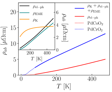
Figure 2: Comparison of $T-$dependence of in-plane resistivity between experiments [23] (dotted lines) and theoretical model in Eq. (1) (solid lines). The only free parameters in the fits are the phonon frequencies and bare el-ph and EME couplings. All other parameters are fixed; see [28, 39]. For the phonon data, we have used $\omega_{D}=29$meV, $\omega_{0}=120$meV, $\widetilde{\omega}_{0}=40$meV, $\lambda_{\rm{el-ph,a}}=0.04$, $\lambda_{\rm{el-ph,o}}=0.02$, $\lambda_{\rm EME}=0.05$ and $S=3/2$.

Role of acoustic phonons.- Our discussion thus far has focused on the simplified limit of an EME coupling to optical phonons. Let us now analyze the effects of an EME coupling to an acoustic phonon. For $H_{\text{ph}}$ in Eq. 1e, this amounts to replacing $\widetilde{\omega}_{0}^{2}\left(\widetilde{\varphi}^{(O)}_{\bm{q}}\right)^{2}\rightarrow\widetilde{\omega}^{2}_{\bm{q}}\left(\widetilde{\varphi}^{(O)}_{\bm{q}}\right)^{2}$, where $\widetilde{\omega}_{\bm{q}}=\widetilde{c}q$ in the limit of small $q$. Similarly, for $H_{\text{EME}}$ in Eq. 1g, this amounts to replacing $\varphi^{(O)}_{i}\to\nabla\varphi^{(O)}_{i}$. Note that, in practice, the out-of-plane vibrations that couple the layers are at a finite wavevector, namely, $\omega_{\bm{q}}\approx\sqrt{\widetilde{c}^{2}q_{x}^{2}+\widetilde{c}^{2}q_{y}^{2}+\widetilde{c}_{z}^{2}q_{z,0}^{2}}$ in the limit where $\widetilde{c}_{z}q_{z,0}\ll T$. It is worth noting that unlike the conventional electron-phonon interaction, where scattering is mainly small-angle up to the BG temperature, the EME term induces large-angle scattering even at low-$T$ due to large momentum transfer to the local-moments, which serve as a “bath”. If the spin structure-factor exhibits non-trivial correlations in the Brillouin-zone (i.e. the spin-correlation length is finite with remnants of Bragg-like peaks), the intermediate-scale transport behavior is controlled by the Pd-electron Fermi-surface geometry. However, when the spin-correlation length is short, $1/\tau_{\rm EME}$ shows two distinct regimes [39]. For $T\gtrsim\widetilde{T}_{\rm BG}\equiv 2\widetilde{c}k_{F}$, the Bloch-Grüneisen temperature, the result reduces to the case of optical phonons, $1/\tau_{\rm EME}=2\pi\lambda_{\rm EME}T$ with $\lambda_{\rm EME}=\frac{\nu_{0}\widetilde{\alpha}^{2}}{M\widetilde{c}^{2}}S(S+1)$. On the other hand, for $J_{\rm H}\lesssim T\lesssim\widetilde{T}_{\rm BG}$, we encounter an unexpected $1/\tau_{\rm EME}=2\pi\lambda_{\rm EME}T^{2}/\widetilde{T}_{\rm BG}$, instead of the usual $\sim T^{4}$ regime in two-dimensions for the phase-space reasons introduced above. Interestingly, this is an example of a $T^{2}$ “quasielastic” scattering due to the EME term (instead of the usual $T^{2}$ due to umklapp scattering).

Effect of $c$-axis strain on in-plane transport.- Given that the proposed EME interaction in PdCrO₂ originates from fluctuations of the (inter-layer) Kondo coupling, applying $c$-axis pressure is expected to enhance the slope of the $T$–linear resistivity for the following reason. The bare EME coupling is controlled in part by the Kondo-scale, $\widetilde{\alpha}\propto t_{cp}^{2}/U$ where $t_{cp}$ is the inter-plane hybridization between the Pd and Cr-electrons and $U$ is the on-site Coulomb repulsion for Cr-electrons [28, 39]. Upon applying $c$-axis strain, the inter-layer distance reduces, thereby increasing $t_{cp}$, which is exponentially sensitive to the deformation; the stiffening of the out-of-plane phonons is at best algebraic. Therefore, the dimensionless EME coupling, $\lambda_{\rm EME}\propto t^{4}_{cp}/(U\widetilde{\omega}_{0})^{2}$ is expected to show a significant increase, along with an enhancement of the Kondo coupling which affects the constant shift in the resistivity at high $T$. The predicted form of the in-plane transport is depicted in the inset of Fig. 3(b) for a range of $c-$axis strain ($\varepsilon_{zz}$) for bare microscopic parameters as chosen in Fig. 2.

Out-of-plane transport.- The electrical resistivity along the $c$-axis provides a direct window into the inter-layer nature of the magnetic interactions, which we have absorbed so far in the effective 2D model. We consider the leading contributions to the $c$-axis conductivity within linear-response theory, which is given by

$$\sigma_{c}=\sigma_{\rm coh}+\sigma_{\rm K}+\sigma_{\rm EME},$$ (6)

where $\sigma_{\rm coh}$ arises from the “coherent” channel due to inter-layer $p$ to $p$ hoppings ($t_{pp}$), and $\sigma_{\rm K}$, $\sigma_{\rm EME}$ represent the “incoherent” channels due to inter-layer spin-assisted and spin-phonon-assisted contributions, respectively [39]. For simplicity, we ignore the contribution due to an interlayer “incoherent” phonon-assisted hopping not involving the local moments; such a term does not affect our results at a qualitative level. The leading-order Feynman diagrams corresponding to each of these contributions are depicted in Fig. 3(a). We have $\sigma_{\rm coh}=e^{2}(n/m)_{c}\tau_{\rm tr}$, where $(n/m)_{c}$ is related to the $c$-axis dispersion and $\tau_{\rm tr}$ is given by Eq. (2); the detailed expressions for the incoherent channels appear in [39].

The coherent channel dominates $\sigma_{c}$ up to temperatures $T\lesssim T_{*}\sim 10^{3}\leavevmode\nobreak\$K (determined by the condition $\sigma_{\rm coh}(T_{*})\approx\sigma_{\rm EME}(T_{*})$ [39]), such that, in this $T$-regime, $\sigma_{c}$ and $\sigma_{ab}$ follow the same $T$-scaling as they share the same transport lifetime. The contribution of the incoherent channels becomes significant at temperatures $T\gtrsim T_{*}$, where, due to the weak $c$-axis dispersion, their temperature dependence is determined by the $T$-scaling of the current vertices, rather than the transport lifetime. In particular, for $T\gtrsim\omega_{D},\widetilde{\omega}_{0}$, while $\sigma_{\rm coh}\sim 1/T$ as in the in-plane case, $\sigma_{\rm K}$ is independent of $T$ and $\sigma_{\rm EME}\propto T$. As a result, the $c$-axis resistivity becomes sublinear at sufficiently high temperatures, as depicted in Fig. 3(b).

The interplay between the different conduction mechanisms has signatures in the behavior under c-axis pressure. The in-plane conductivity is expected to decrease with $c-$axis compression, since the EME scattering is enhanced (because it is proportional to the inter-plane hopping strength.) In contrast, the coherent part of the $c-$axis conductivity increases, as a result of the enhanced inter-layer hopping [39]. Interestingly, this increase in $\sigma_{\rm coh}$ is associated solely with the el–ph scattering term. The contributions to $\sigma_{\rm coh}$ from the Kondo and EME terms are proportional to $t_{pp}^{2}/t_{cp}^{4}$ [39]; assuming that $t_{pp}\propto t_{cp}^{2}$, the ratio $t_{pp}^{2}/t_{cp}^{4}$ is unchanged by $c-$axis strain. Similarly, the incoherent parts of the conductivity increase with compression. However, they do so slightly in excess of $\sigma_{\rm coh}$ which in turn reduces the crossover scale $T_{*}$, as manifested by the increase in curvature at intermediate temperatures with increasing compression; see Fig. 3(b) [39]. There are measurements of the $c-$axis resistivity in the literature [60, 61], but the reported values are inconsistent with each other. The reason for this discrepancy is currently unclear. To resolve these issues, more accurate measurements are needed, using e.g. the techniques described in Ref. [62].

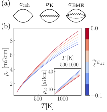
Figure 3: (a) The Feynman diagrams contributing at leading-order to the $c-$axis conductivity, $\sigma_{c}$ (see Eq. (6)), where solid, wiggly and dashed lines denote electrons, spins and phonons, respectively. (b) $c$-axis resistivity as a function of $T$ for different (compressive) $c$-axis strain $\varepsilon_{zz}$ (in units of $\xi/a_{z}$, where $\xi$ is the characteristic decay length of the hopping integral and $a_{z}$ is the $\hat{z}$ lattice constant). Inset: in-plane resistivity as a function of $T$ under $c$-axis strain $\varepsilon_{zz}$.

Discussion.- Our conjectured magneto-elastic mechanism for the enhanced $T-$linear resistivity in PdCrO₂ relies on quasi-elastic scattering, where the phonons are in the equipartition regime. There is experimental evidence for the Lorenz ratio satisfying the Wiedemann-Franz law in the $T-$linear regime [31], which is consistent with our mechanism. Interestingly, the extracted transport scattering rate in the same regime of $T-$linear resistivity is Planckian with $C\approx 0.9$ [31]. Within our model and in the quasi-elastic regime, this is not indicative of any fundamental principle, such as a bound associated with an inelastic scattering rate. It is, however, far from obvious why the scattering rate turns out to be Planckian.

A natural future direction is to study the effects of the EME term at low temperature. In particular, the magneto-elastic coupling might be evident in the electronic spectral function. Signatures of phonon drag observed in PdCoO₂ [58] are expected to be suppressed in PdCrO₂ due to EME-induced large-angle scattering of phonons off magnetic moments [25]. Pronounced magnetic correlations may also lead to a generalized Kohn anomaly [63] associated with phonon softening at the AFM wavevectors. A detailed understanding of the low-temperature properties of this interesting system remains an open problem.

Acknowledgements- JFMV and DC acknowledge the hospitality of the Weizmann Institute of Science, where this work was completed. JFMV and DC thank A. McRoberts and R. Moessner for an earlier related collaboration [40] and insightful discussions. DC thanks P. Coleman, J. Ruhman, and T. Senthil for useful discussions. JFMV and DC are supported in part by a CAREER grant from the NSF to DC (DMR-2237522). DC and EB acknowledge the support provided by the Aspen Center for Physics where this collaboration was initiated, which is supported by National Science Foundation grant PHY-1607611. Research in Dresden benefits from the environment provided by the DFG Cluster of Excellence ct.qmat (EXC 2147, project ID 390858940).

Appendix A Derivation of the EME coupling

We derive the low-energy effective Kondo lattice model with EME term starting from an Anderson-type model coupled to phonons; the Kondo term was already derived in Ref. [28]. The key new insight is as follows: the effective Kondo-like coupling that is generated between the Pd-electrons and Cr local moments involves an inter-layer hybridization, $t_{cp,ij}$ between sites $i$ and $j$. If this coupling were to be affected by the fluctuations associated with the corresponding out-of-plane bond, $t_{cp,ij}$ will be renormalized by the displacement, $\varphi^{(O)}_{ij}$. Starting with the microscopic Hamiltonian,

$$H =H_{\text{Pd}}+H_{\text{Cr}}+H_{\text{hyb}}+H_{\text{ph,EME}},$$ (7)

$$H_{\text{Pd}} =\sum_{\bm{k}\sigma}\left(\varepsilon_{\bm{k}}-\mu\right)p_{\bm{k}\sigma}^{\dagger}p_{\bm{k}\sigma},$$ (8)

$$H_{\text{Cr}} =-\sum_{ij\sigma}t_{ij}^{c}c_{i}^{\dagger}c_{j}+\text{h.c}+U\sum_{i}\left(n_{i\uparrow}^{c}-\frac{1}{2}\right)\left(n_{i\downarrow}^{c}-\frac{1}{2}\right),$$ (9)

$$H_{\text{hyb}} =\sum_{\left\langle ij\right\rangle\sigma}t_{cp,ij}\left(1-\eta\varphi^{(O)}_{ij}\right)\left(c_{i\sigma}^{\dagger}p_{j\sigma}+\text{h.c}\right)$$ (10)

$$H_{\text{ph,EME}} =\sum_{\left\langle ij\right\rangle}\frac{\pi_{ij}^{(O)\,2}}{2M}+\frac{M\tilde{\omega}_{0}}{2}\varphi_{ij}^{(O)\,2},$$ (11)

where $c,\leavevmode\nobreak\ c^{\dagger}$ represent the Cr-electron operators, $t_{ij}^{c}$ is a nearest-neighbor hopping in the Cr layer, $\varepsilon_{\bm{k}}$ is the dispersion for the Pd electrons, $\eta$ determines the scale by which the hybridization is renormalized to leading order in the bond displacement $\varphi^{(O)}_{ij}$, $M$ is the phonon mass, $n_{i\sigma}^{c}$ is the density operator for Cr electrons, and $U$ is the on site interaction strength. In general, these interactions involve multiple orbitals associated with the Cr crystal field multiplets, and contain the full lattice structure of PdCrO₂. However, here for simplicity, we only retain a single orbital per site in the Cr layers.

We consider the strong-coupling limit, $U\gg t^{c},g$ (similarly to Ref. [28]), and derive the low-energy model based on a Schriffer-Wolff transformation. Retaining terms up to linear-order in the bond displacement, we obtain:

$$H =H_{\text{Pd}}+H_{\text{lm}}+H_{\text{K}}+H_{\text{EME}}+H_{\text{ph,EME}},$$ (12)

$$H_{\text{lm}} =J_{H}\sum_{\left\langle ij\right\rangle}\bm{S}_{i}\cdot\bm{S}_{j}$$ (13)

$$H_{\text{K}} =\sum_{\left\langle ilj\right\rangle\sigma}\frac{4t_{cp,ij}t_{cp,lj}}{U}\bm{S}_{l}\cdot\left(p_{i}^{\dagger}\bm{\sigma}p_{j}\right)$$ (14)

$$H_{\text{EME}} =-\sum_{\left\langle ilj\right\rangle\sigma}\frac{4t_{cp,ij}t_{cp,lj}}{U}\eta\left(\varphi^{(O)}_{il}+\varphi^{(O)}_{jl}\right)\bm{S}_{l}\cdot\left(p_{i}^{\dagger}\bm{\sigma}p_{j}\right)$$ (15)

The first term above is the usual Heisenberg coupling with antiferromagnetic exchange $J_{H}=4(t^{c})^{2}/U$. The second term is a Kondo coupling [28] with the appropriate form-factors coming from the fact that the interaction is inter-layer. The third term is the new EME coupling between local moments in the Cr layer, optical phonons and itinerant Pd-electrons. In what follows, we consider the simplified case where the adjacent Pd layers are stacked in a perfectly aligned arrangement, and the hybridization is independent of the bond direction, i.e. $t_{cp,ij}\rightarrow t_{cp}$. In this limit, we can define the Kondo and EME couplings to be $J_{K}=4t_{cp}^{2}/U$ and $\tilde{\alpha}=-J_{K}\eta$. We then have the following Hamiltonian in momentum space

$$H=H_{\text{Pd}}+H_{\text{ph}}+H_{\text{lm}}+H_{\text{int}}$$ (16)

with the interaction given by

$$H_{\text{int}}= \frac{1}{\sqrt{N}}\sum_{\begin{subarray}{c}\bm{k}\bm{k}^{\prime}\\ \alpha\beta\end{subarray}}J_{K}\left(\bm{k},\bm{k}^{\prime}\right)p_{\bm{k}\alpha}^{\dagger}\left[\bm{S}_{\bm{k}-\bm{k}^{\prime}}\cdot\bm{\sigma}_{\alpha\beta}\right]p_{\bm{k}^{\prime}\beta}$$ (17)

$$+\frac{1}{N}\sum_{\bm{k}\bm{k}^{\prime}\bm{q}}\sum_{\ell\alpha\beta}\tilde{\alpha}_{\ell}\left(\bm{k},\bm{k}^{\prime}\right)\varphi^{(O)}_{\ell}\left(\bm{k}-\bm{k}^{\prime}-\bm{q}\right)p_{\bm{k}\alpha}^{\dagger}\left[\bm{S}_{\bm{q}}\cdot\bm{\sigma}_{\alpha\beta}\right]p_{\bm{k}^{\prime}\beta}$$ (18)

where the Fourier transformed operators are:

$$\varphi^{(O)}_{\ell+j,j}=\frac{1}{\sqrt{N}}\sum_{\bm{k}}e^{-i\bm{k}\bm{R}_{j}}\varphi^{(O)}_{\ell}\left(\bm{k}\right)$$ (19)

$$p_{i\alpha}^{\dagger}=\frac{1}{\sqrt{N}}\sum_{\bm{k}}e^{-i\bm{k}\bm{R}_{i}}p_{\bm{k}\alpha}^{\dagger}$$ (20)

$$\bm{S}_{j}=\frac{1}{\sqrt{N}}\sum_{\bm{q}}e^{-i\bm{q}\bm{R}_{j}}\bm{S}_{\bm{q}}$$ (21)

and the momentum-dependent couplings are

$$J_{K}\left(\bm{k},\bm{k}^{\prime}\right) =J_{K}\left[2\cos\left(k_{z}a_{z}\right)\right]\left[2\cos\left(k_{z}^{\prime}a_{z}\right)\right]$$

$$\tilde{\alpha}_{+1}\left(\bm{k},\bm{k}^{\prime}\right) =\tilde{\alpha}_{-1}\left(\bm{k},\bm{k}^{\prime}\right)=\tilde{\alpha}\left(\bm{k},\bm{k}^{\prime}\right)=-\eta J_{K}\left(\bm{k},\bm{k}^{\prime}\right),$$

with $\bm{R}_{i}$ being the position of site $i$ and $N$ the number of unit cells.

We have introduced three new parameters: the mass of the out-of-plane mode $M$ (appearing in the EME term), its frequency $\tilde{\omega}_{0}$ and the EME coupling $\eta$. As we detail in the text, these parameters only enter the theory either in the precise combination that corresponds to the dimensionless EME coupling, or in the combination $\beta\tilde{\omega}_{0}$, leaving effectively two new parameters in the theory. The rest of the parameters are taken from the values provided in [28]. Specifically, we have $U=4$eV and $t_{cp}=107$meV which lead to a Kondo coupling of $J_{K}=11.45$ meV. Additionally, we have $J_{H}=6.25$meV, $t_{nn}^{p}=568$meV, $t_{nnn}^{p}=108$meV, and $\mu=256$meV. We fit the difference of the resistivity of PdCrO₂ and PdCoO₂ to obtain the dimensionless EME coupling in the main text and the frequency of this mode.

Appendix B Transport rate

Within the variational Boltzmann approach [8] the transport lifetime can estimated by

$$\rho\leq\frac{\frac{V}{2k_{B}T}\sum_{\bm{q}\bm{p}}P_{\bm{p}\bm{q}}\left(\psi_{\bm{q}}-\psi_{\bm{p}}\right)^{2}}{\left|\sum_{\bm{q}}e\frac{\partial f}{\partial\epsilon_{\bm{q}}}\psi_{\bm{q}}\bm{v}\left(\bm{q}\right)\cdot\bm{n}\right|^{2}}$$ (22)

with $\psi_{\bm{q}}$ a variational anzatz, $P_{\bm{p}\bm{q}}$ the transition probaility from different momentum states, $V$ the volume, $\bm{n}$ is a unit vector in the direction of the electric field $\bm{E}$, $f$ the Fermi-Dirac distribution, $e$ the electron charge, $\bm{v}\left(\bm{q}\right)=\partial_{\bm{q}}\epsilon_{\bm{q}},$ and $\epsilon_{\bm{q}}$ the dispersion. Using the ansatz $\psi_{\bm{q}}=-e\bm{v}_{\bm{q}}\cdot\bm{E}\tau_{\text{tr}}$ we recover the drude formula with the momentum relaxation time

$$\tau_{\text{tr}}^{-1}=\frac{\frac{1}{k_{B}T}\sum_{\bm{q}\bm{p}}P_{\bm{p}\bm{q}}\left(\bm{v}\left(\bm{q}\right)\cdot\bm{n}-\bm{v}\left(\bm{q}\right)\cdot\bm{n}\right)^{2}}{\sum_{\bm{q}}2\left(-\frac{\partial f}{\partial\epsilon_{\bm{q}}}\right)\left(\bm{v}\left(\bm{q}\right)\cdot\bm{n}\right)^{2}}.$$ (23)

At intermediate-$T$, where the scattering mechanisms are essentially isotropic, Mathiessen’s rule is obeyed such that

$$\tau_{\text{tr}}^{-1}=\tau_{\text{K}}^{-1}+\tau_{\text{EME}}^{-1}+\tau_{\text{el--ph}}^{-1}$$ (24)

where each individual scattering rate is determined by the transition probabilities

$$P_{\bm{p}\bm{q}}^{\rm{K}}=k_{B}T\frac{2\pi}{\hbar}\left(-\frac{\partial f_{\bm{p}}}{\partial\epsilon_{\bm{p}}}\right)\left|J_{K}\left(\bm{p},\bm{q}\right)\right|^{2}\chi^{\prime\prime}\left(\bm{p}-\bm{q},\varepsilon_{\bm{p}}-\epsilon_{\bm{q}}\right)\left(n_{B}\left(\varepsilon_{\bm{p}}-\epsilon_{\bm{q}}\right)+n_{F}\left(-\epsilon_{\bm{q}}\right)\right),$$ (25)

$$P_{\bm{k}\bm{p}}^{\rm{EME}}=k_{B}T\frac{2\pi}{\hbar}\left(-\frac{\partial f}{\partial\epsilon_{\bm{p}}}\right)\left|\tilde{\alpha}\left(\bm{p},\bm{q}\right)\right|^{2} \sum_{\bm{k}}\int\frac{d\nu}{\pi}\chi^{\prime\prime}\left(\bm{k}+\bm{p}-\bm{q},\epsilon_{\bm{p}}-\nu\right)\mathcal{B}\left(\bm{k},\nu-\varepsilon_{\bm{q}}\right)\times$$

$$\left[n_{B}\left(\epsilon_{\bm{p}}-\nu\right)+n_{F}\left(-\nu\right)\right]\left[n_{B}\left(\nu-\varepsilon_{\bm{q}}\right)+n_{F}\left(-\varepsilon_{\bm{q}}\right)\right],$$ (26)

$$P_{\bm{p}\bm{q}}^{\rm{el-ph}}=kT\frac{2\pi}{\hbar}\left(-\frac{\partial f_{\bm{p}}}{\partial\epsilon_{\bm{p}}}\right)\sum_{\lambda}\left|\alpha_{\lambda}\left(\bm{p},\bm{q}\right)\right|^{2}\mathcal{B}_{\lambda}\left(\bm{p}-\bm{q},\varepsilon_{\bm{p}}-\epsilon_{\bm{q}}\right)\left(n_{B}\left(\varepsilon_{\bm{p}}-\epsilon_{\bm{q}}\right)+f\left(-\epsilon_{\bm{q}}\right)\right).$$ (27)

Here $\chi^{\prime\prime}\left(\bm{p},\omega\right)$ is the spin susceptibility and $\mathcal{B}_{\lambda}\left(\bm{k},\nu\right)$ is the phonon spectral function for mode $\lambda=o,a$ which can be either acoustic or optical. We also reintroduced the momentum dependence in all the couplings. In the case where the magnetic and itinerant electron layers are perfectly aligned we have

$$J_{K}\left(\bm{p},\bm{q}\right)=J_{K}\left[2\cos\left(p_{z}a_{z}\right)\right]\left[2\cos\left(q_{z}a_{z}\right)\right],$$ (28)

$$\tilde{\alpha}\left(\bm{p},\bm{q}\right)=\tilde{\alpha}\left[2\cos\left(p_{z}a_{z}\right)\right]\left[2\cos\left(q_{z}a_{z}\right)\right],$$ (29)

$$\alpha_{\rm{o}}\left(\bm{p},\bm{q}\right)=\alpha_{\rm{o}},$$ (30)

and

$$\alpha_{\rm{a}}\left(\bm{p},\bm{q}\right)=\alpha_{\rm{a}}\left|\bm{p}-\bm{q}\right|.$$ (31)

Here the coupling constants are as defined in the main text. Additionally, we make the local approximation for the spins [40]:

$$\chi^{\prime\prime}\left(\nu\right)=S\left(S+1\right)\beta\nu\frac{\theta\left(2\pi J_{H}-\left|\nu\right|\right)}{2J_{H}}$$ (32)

with the sum rule constraint

$$\int\frac{\chi^{\prime\prime}\left(\nu\right)}{\beta\nu}d\nu=2\pi S\left(S+1\right).$$ (33)

The spectral function for the free phonons is given by

$$\mathcal{B}_{\lambda}\left(\bm{k},\nu\right)=\frac{\pi\hbar}{2M\omega_{\bm{k},\lambda}}\left(\delta\left(\nu-\omega_{\bm{k},\lambda}\right)-\delta\left(\nu+\omega_{\bm{k},\lambda}\right)\right)$$ (34)

where for optical phonons we have $\omega_{\bm{k},o}=\omega_{0}$ while for acoustic phonons $\omega_{\bm{k},a}=ck$. The integrals above can then be evaluated analytically if we take a quasi-2D circular fermi surface. This leads to the total scattering rate:

$$\tau_{\rm{tr}}^{-1} =2\pi\frac{\lambda_{tr,\rm{EP},o}}{\hbar\beta}\mathcal{I}_{1}\left(\frac{\beta\hbar\omega_{0}}{2}\right)+2\pi\frac{\lambda_{tr,\rm{EP},a}}{\hbar\beta}\mathcal{I}_{2}\left(\frac{\beta\hbar\omega_{BG}}{2}\right)$$

$$+2\pi\frac{\lambda_{K}J_{\rm{K}}}{\hbar}\mathcal{I}_{3}\left(2\pi\beta J_{\rm{H}}\right)+2\pi\frac{\lambda_{tr,\rm{EME}}}{\hbar\beta}\mathcal{I}_{4}\left(2\pi\beta J_{\rm{H}},\beta\hbar\tilde{\omega}_{0}\right)$$ (35)

Here we define

$$\mathcal{I}_{1}\left(x\right)=\left[x\text{csch}\left(x\right)\right]^{2},$$ (36)

and

$$\mathcal{I}_{2}\left(x\right)=\frac{4}{\pi}\frac{1}{x^{3}}\int_{0}^{x}dy\ \frac{y^{4}}{\sqrt{1-\left(\frac{y}{x}\right)^{2}}}\left[\text{csch}\left(y\right)\right]^{2},$$ (37)

corresponding to the case of acoustic phonons interacting with a circular Fermi surface in two dimensions. In addition,

$$\mathcal{I}_{3}\left(y\right) =-\frac{4\text{Li}_{2}\left(e^{-y}\right)}{y}-\frac{2y}{e^{y}-1}-4y+\frac{2\pi^{2}}{3y}+4\log\left(e^{y}-1\right),$$ (38)

corresponds to the pure Kondo scattering at high temperatures, where the logarithmic integrals result from integrating the Fermi function. And finally

$$\mathcal{I}_{4}\left(y,z\right)=\frac{z^{2}}{\cosh\left(z\right)-1}\mathcal{J}\left(y,z\right)$$ (39)

is the result of the integrals involving the EME coupling, with the additional definition:

$$\mathcal{J}\left(y,z\right) =\frac{-2z\text{Li}_{2}\left(e^{-y}\right)+\left(2y+z\right)\text{Li}_{2}\left(e^{-y-z}\right)+\left(z-2y\right)\text{Li}_{2}\left(e^{z-y}\right)+2\text{Li}_{3}\left(e^{-y-z}\right)-2\text{Li}_{3}\left(e^{z-y}\right)}{2yz}$$

$$+\frac{z^{2}}{12y}-\frac{1}{2}\log\left(\left(e^{y}-e^{z}\right)\left(e^{y+z}-1\right)\right)+\frac{y\log\left(\sinh\left(\frac{y-z}{2}\right)\text{csch}\left(\frac{y+z}{2}\right)\right)}{2z}+\frac{y}{2}+\frac{\pi^{2}}{3y}+\log\left(e^{y}-1\right)+\frac{z}{2}.$$ (40)

These functions have the following high temperature limits which can be obtained from the asymptotic expansions for the polylogarithm

$$\lim_{T\rightarrow\infty}\mathcal{I}_{1}\left(\frac{\beta\hbar\omega_{0}}{2}\right)=\lim_{T\rightarrow\infty}\mathcal{I}_{2}\left(\frac{\beta\hbar\omega_{BG}}{2}\right)=1$$ (41)

and

$$\lim_{T\rightarrow\infty}\mathcal{I}_{3}\left(2\pi\beta J_{H}\right)=\lim_{T\rightarrow\infty}\mathcal{I}_{4}\left(2\pi\beta J_{H},\beta\hbar\tilde{\omega}_{0}\right)=2.$$ (42)

In the main text, we use the effective mass of PdCoO₂ extracted from quantum oscillations given in Ref. [64], and the density corresponding to half filling to extract the transport rate from experiments following the procedure in Ref. [3] to calculate the ratio $n/m$ for both PdCoO₂ and PdCrO₂. Then we fit the resulting scattering rate to the first two terms which correspond to electron-phonon scattering in $\tau_{tr}^{-1}$. With this procedure, we find the parameters $\lambda_{\rm el-ph,o}=0.024$,$\hbar\omega_{0}=120$meV,$\lambda_{\rm el-ph,a}=0.043$, and $\hbar\omega_{\rm BG}=29$meV, which are in close agreement with the reported values in [58, 59]. The difference between our treatment and that in Refs. [58, 59] is that we consider a 2D fermi surface instead of a 3D Fermi surface. At intermediate temperatures where our theory is valid we do not see significant differences in the fit quality between the model considered here and the ones in [58, 59] .

We then carry out the same procedure for PdCrO₂ and substract the resulting scattering rate from the scattering rate extracted from PdCoO₂. This would isolate the last two terms that correspond to Kondo and EME scattering in $\tau_{tr}^{-1}$. By fitting this excess scattering rate we find the EME parameters $\lambda_{\rm EME}=0.025$ and $\hbar\tilde{\omega}_{0}=45$meV. Since we use the high temperature approximation for $\chi^{\prime\prime}$ we do not fit the low temperature regime of $\Delta_{\tau}=\tau_{\rm{tr,Cr}}^{-1}-\tau_{\rm{tr,Co}}^{-1}$ but only carry the fit at temperatures above 80K ($J_{H}\sim 72K$). Note that the constant offset between the PdCoO₂ and the PdCrO₂ resistivities is not fitted. This excess scattering rate comes purely from the Kondo scattering with the dimensionless coupling $\lambda_{K}=4S\left(S+1\right)J_{K}\nu_{0}$ and a saturation scale set by $J_{H}$, where the value of these couplings is listed above.

In the above, one can trace the variuous features of $\rho$ for PdCrO₂ to each of the terms in Eqn. 35.The Kondo term increases sharply and completely saturates at a temperature scale set by $2\pi J_{H}$. This approach to saturation would be responsible for the sublinear approach to the $T$–linear regime. This sublinear piece dominates at $T\sim J_{H}$ over the contributions from the phonon and the magnetoelastic scattering rates. Eventually, both of these contributions catch up with the Kondo scattering rate and the resistivity becomes $T$–linear which can be seen from the high temperature limits of $\mathcal{I}_{4}$ and $\mathcal{I}_{3}$ and the expression for $\tau_{tr}^{-1}$. Taking the high temperature limit, we can determine the coefficient of the linear in $T$ scattering rate. Using the asymptotic expressions above and the values of the fitted dimensionless couplings we get

$$\lim_{T\rightarrow\infty}\frac{d}{dT}\tau_{\rm{tr}}^{-1} =\left(\frac{k_{B}}{\hbar}\right)2\pi\left(\lambda_{\rm el-ph,o}+\lambda_{\rm el-ph,a}+2\lambda_{\rm EME}\right)$$ (43)

$$\sim 0.75\left(\frac{k_{B}}{\hbar}\right)$$ (44)

which is close to the Planckian slope $k_{B}/\hbar$.

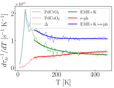
Supplemental Figure S1: Rate of change of the scattering rates from fit and experiments. In the case where the resistivity is completely saturated we expect this quantity to be constant. However, neither the electron-phonon contribution, nor the Kondo and EME contributions are linear. Nevertheless, the sum of the scattering rates is almost linear, as evidenced by the constant rate of change.

Finally, we note that neither $\tau_{\rm el-ph}^{-1}$ nor $\tau_{\rm K}^{-1}$ are in the fully saturated regime for the values of the fit parameters obtained from the above procedure (see Fig. S1). In contrast, the excess resistivity from the EME term is generated by a mode that saturates at relatively low temperatures (since the out-of-plane vibration in PdCrO₂ turns out to be softer than the in-plane one). At the same time, the addition of the pure Kondo scattering gives an additional $T$-sublinear contribution to the resistivity. In total, the $T$-superlinear scattering rate from electron-phonon scattering and the $T$-sublinear contribution from the Kondo term, together with the $T$-linear EME contribution yield an approximately $T$–linear resistivity for PdCrO₂.

Appendix C Out-of-plane resistivity

The starting point of our discussion is a slightly modified version of the model introduced in the discussion of in-plane transport. Here, we assume that in addition to the regular in-plane hopping in the Pd layer, we have a small but non negligible hopping $t_{pp}$ between adjacent Pd layers. The value of this hopping parameter is estimated to be $\sim 0.042t^{p}_{nn}$ by taking as a reference the dispersion of PdCoO₂ as measured by quantum oscillations [58]. Once this hopping has been introduced, the current operator in the $z$ direction can be readily calculated. This operator has three distinct contributions (ignoring for simplicity the phonon-assisted, but local-moment independent, term):

$$\bm{J}^{0} = -i\sum_{ij\sigma}t^{p}_{ij}\left(\bm{r}_{i}-\bm{r}_{j}\right)p_{i\sigma}^{\dagger}p_{j\sigma}$$ (45)

$$\bm{J}^{1} = -i\frac{J_{K}}{2}\sum_{ilj\beta\alpha}\left(\bm{r}_{i}-\bm{r}_{j}\right)p_{i\alpha}^{\dagger}\left(\bm{S}_{l}\cdot\bm{\sigma}_{\alpha\beta}\right)p_{j\beta}$$ (46)

$$\bm{J}^{2} = i\frac{\eta J_{K}}{2}\sum_{ilj\beta\alpha}\left(\varphi^{(O)}_{il}+\varphi_{jl}^{(O)}\right)$$ (47)

$$\,\,\,\,\,\,\,\,\,\,\,\,\,\,\,\,\,\,\,\,\times\left(\bm{r}_{i}-\bm{r}_{j}\right)p_{i\alpha}^{\dagger}\left(\bm{S}_{l}\cdot\bm{\sigma}_{\alpha\beta}\right)p_{j\beta}$$

where $\bm{J}^{0}$ is the usual current operator that has a $z$ component induced by $t_{pp}$, $\bm{J}^{1}$ is an assisted hopping current mediated by a local moment $\bm{S}_{l}$ at site $\bm{r}_{l}$ in the Cr layer, and $\bm{J}^{2}$ is a phonon and local moment assisted hopping, with $\varphi^{(O)}_{il}$ being the bond stretching displacement between sites at $\bm{r}_{i}$ in a Pd layer and $\bm{r}_{l}$ in a Cr layer. For the in-plane transport, these conduction channels are usually shorted by the coherent current $\bm{J}^{0}$ due to the large in-plane Fermi velocity, which is why they were absent from our previous discussions. However, these terms are relevant in the discussion of c-axis resistivity, since the hopping integral $t_{pp}$ is now of similar magnitude as the Kondo and EME couplings which set the overall scale of the incoherent currents.

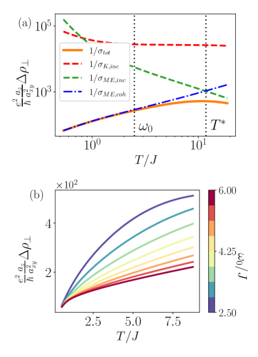
Supplemental Figure S2: c-axis transport: (a) different contributions to the c-axis resistivity for a soft phonon frequency $\omega_{0}=2.5J_{H}$. Coherent transport dominates over a broad temperature regime but deviates from $T$ linearity at a temperature $T_{*}$ set by the electron velocity and the magnetoelastic coupling (see main text). The pure incoherent Kondo scattering is always shorted by other conducton channels. (b) Dependence of the c-axis resistivity on variations of the phonon frequency. As $\omega_{0}$ becomes softer the incoherent conductivty is enhanced and the coherent scattering increases making a saturation regime accessible at high temperatures.

To calculate the conductivity we compute the current-current correlation for the total current $\bm{J}=\sum_{i}\bm{J}^{i}$. Since we work perturbatively in the Kondo and EME couplings, as well as in the out-of-plane hopping $t_{pp}$, the cross correlations between different current operators are subleading and we obtain

$$\sigma^{c} = \sigma_{\text{inc}}+\sigma_{\text{coh}}$$ (48)

$$\sigma^{c}_{\text{inc}} = \lim_{\omega\rightarrow 0}\lim_{\bm{q}\rightarrow 0}\sum_{i=1,2}\frac{-1}{\beta V}\langle J^{i}_{z}(\tilde{q})J^{i}_{z}(-\tilde{q})\rangle$$ (49)

$$\sigma^{c}_{\text{coh}} = 4e^{2}t_{pp}^{2}a_{z}^{2}\nu_{0}\langle\tau_{\rm{tr}}\sin^{2}k_{z}a_{z}\rangle$$ (50)

where $\langle\cdot\rangle$ denotes the momentum average over the Fermi surface, and $\nu_{0}$ is the density of states at the Fermi level. The behavior of each individual contribution to the conductivity is shown in Fig. S2(a). Here we see that the incoherent contribution from the Kondo current $\bm{J}^{1}$ to the resistivity decreases with increasing $T$ and then saturates at a scale set by $J_{\rm H}$. In contrast the contribution of the EME current $\bm{J}^{2}$ to the resistivity continues to decrease with temperature with $\rho_{\text{inc, EME}}\sim T^{-1}$. At the same time the coherent contribution rises with temperature $\rho_{\text{coh}}\sim T$. We then obtain the total resistivity from parallel addition of each individual conduction channel. Interestingly, we note that there is a crossover temperature scale $T_{*}$ at which the incoherent and coherent resistivities coincide. At this scale, we expect resistivity saturation. At asymptotically high temperatures, there is an eventual change of trend where the resistivity decreases as a function of temperature as a consequence of incoherent processes.

To estimate the scale at which this crossover occurs, we simply equate the high temperature limits of $\sigma^{c}_{\text{inc}}$ and $\sigma^{c}_{\text{coh}}$. Since the incoherent conductivity is dominated by the EME current correlations, we can approximate at high temperatures:

$$\sigma^{c}_{\text{inc}}\sim\left(\frac{a_{z}}{a_{xy}^{2}}\frac{e^{2}}{\hbar}\right)\lambda_{\rm{EME}}\nu_{0}T$$ (51)

In the same regime, the coherent contribution to the conductivity can be well approximated by:

$$\sigma^{c}_{\text{coh}}\sim\left(\frac{a_{z}}{a_{xy}^{2}}\frac{e^{2}}{\hbar}\right)\frac{t_{pp}^{2}\nu_{0}}{(\lambda_{\rm{EME}}+\lambda_{\rm{el-ph}})k_{B}T}.$$ (52)

Equating these two conductivities and estimating $v_{z}\sim t_{pp}a_{z}/\hbar$ we get the crossover temperature

$$T_{*}\sim\frac{v_{z}G_{z}}{\sqrt{\lambda_{\rm{EME}}(\lambda_{\rm{EME}}+\lambda_{\rm{el-ph}})}},$$ (53)

with $G_{z}=2\pi\hbar/a_{z}$. Note that the dependence on the density of states is now hidden in $\lambda_{\rm{EME}}$, which also depends on the frequency of the mode that mediates the EME interaction.

We now analyze the effect of pressure on the $c$-axis resistivity. Specifically, applying compressive strain along the $c$ direction introduces changes in the lattice constants, the hopping integrals, the Kondo coupling, and the phonon frequency. The expectation is that the phonon frequencies and lattice constants change algebraically while $J_{\rm{K}}$ and $t_{pp}$ change exponentially, so we focus on the latter in what follows. Additionally, we have $J_{\rm{K}}\propto t_{cp}^{2}/U,$ with $t_{cp}$ setting the scale of the hybridzation between Cr and Pd layers. Consider the case where $t_{cp}^{2}$ has an exponential dependence on $a_{z}$ similar to that of $t_{pp}$. This could happen, for instance, if the inter-layer hopping is controlled by virtual tunneling via the Cr layers, then $t_{pp}$ is also proportional to $t_{cp}^{2}/U$. As a consequence, $J_{\rm{K}}$ increases at the same rate as $t_{pp}$ when pressure is applied along the $c-$axis. This entails that upon applying pressure, $\sigma^{c}_{\rm inc}$ grows since the overall scale of the incoherent current increased. At the same time, $\sigma^{c}_{\rm{coh}}$ increases since the increase in the $c-$axis velocity is matched by the increase of the scattering rate with decreasing $a_{z}$ for the Kondo and EME contributions, but not for the el–ph contribution.

These changes to the resistivity also have an effect on the crossover scale $T_{*}$. With the scaling of the different hopping parameters, we find that $\lambda_{\rm EME}$ scales with $c$-axis pressure in the same way as $v_{z}^{2}$. Following Eqn. 53, the crossover temperature $T_{*}$ is expected to decrease with increasing pressure. As such, deviations from $T$-linearity in the resistivity are expected to occur at lower temperatures when pressure is applied.

Appendix D Incoherent contribution to the $c$-axis resistivity

To evaluate the incoherent contribution to the conductivity we start by Fourier transforming the current operators that are associated with the Kondo and EME assisted hoppings between Pd layers. These current operators are given by

$$J^{1}_{z}\left(\omega_{n}\right)=\frac{1}{\sqrt{N\beta}}\sum_{\begin{array}[]{c}\bm{k}\bm{k}^{\prime}\alpha\beta\\ i\nu_{l},i\nu_{n}\end{array}}f\left(\bm{k},\bm{k}^{\prime}\right)p_{\bm{k}\alpha}^{\dagger}\left(i\nu_{l}\right)\left[\bm{S}_{\bm{k}-\bm{k}^{\prime}}\left(i\nu_{l}-i\nu_{n}\right)\cdot\bm{\sigma}_{\alpha\beta}\right]p_{\bm{k}^{\prime}\beta}\left(i\nu_{n}+i\omega_{n}\right)$$ (54)

$$J^{2}_{z}\left(\omega_{n}\right) =\frac{1}{N\beta}\sum_{\begin{array}[]{c}\bm{k}\bm{k}^{\prime}\bm{q}\alpha\beta\ell\\ i\nu_{l},i\mu_{m},i\nu_{n}\end{array}}\Lambda_{\ell}\left(\bm{k},\bm{k}^{\prime}\right)\varphi^{(O)}_{\ell,\bm{k}-\bm{k}^{\prime}-\bm{q}}\left(i\nu_{l}-i\mu_{m}-i\nu_{n}\right)p_{\bm{k}\alpha}^{\dagger}\left(i\nu_{l}\right)\left[\bm{S}_{\bm{q}}\left(i\mu_{m}\right)\cdot\bm{\sigma}_{\alpha\beta}\right]p_{\bm{k}^{\prime}\beta}\left(i\nu_{n}+i\omega_{n}\right)$$ (57)

where the bare vertices are given by

$$f\left(\bm{k},\bm{k}^{\prime}\right) =J_{K}\left(\frac{2a_{z}}{\hbar}\right)\sin\left(k_{z}a_{z}+k_{z}^{\prime}a_{z}\right),$$ (58)

and

$$\Lambda_{+}\left(\bm{k},\bm{k}^{\prime}\right) =\Lambda_{-}\left(\bm{k},\bm{k}^{\prime}\right)=-\eta f\left(\bm{k},\bm{k}^{\prime}\right)$$ (59)

we additionally parametrized the magnetoelastic interaction as $\tilde{\alpha}=-J_{k}\eta$ . Note that we have two phonon operators per local moment since there are two bond streching modes, one that connects to the upper and one that connects to the lower Pd layers. With these definitions, we proceed to calculate the current-current correlation functions

$$\Pi_{\bm{k}}^{zz}\left(i\omega_{n}\right)=\frac{-1}{\beta V}\sum_{i}\langle J_{z}^{i}(\tilde{q})J_{z}^{i}(-\tilde{q})\rangle=\Pi_{1}+\Pi_{2}$$ (60)

There are two diagrams that contibute to leading order, these are respectively: diagram

(61)

(62)

where the dotted line corresponds to the $\bm{J}^{1}$ current, the dashed line denotes the spin susceptibility, the zig-zag line is a $\bm{J}^{2}$ current, and the wiggly line is a phonon propagator. Note that there are no other phonon vertices since the interaction is diagonal in the phonon mode. If we allow for anharmonicities, further corrections to the $\Pi_{2}$ correlation function will contribute.

The first diagram above amounts to the following expression:

$$\Pi_{\bm{k},1}^{zz}\left(i\omega_{n}\right)=\frac{1}{\beta V}\frac{1}{\beta N}\sum_{\bm{q}\bm{p}}\sum_{i\nu_{n}iz_{n}}\left|f\left(\bm{p}+\bm{q},\bm{k}+\bm{q}\right)\right|^{2}S\left(\bm{p},iz_{n}\right)\mathcal{G}\left(\bm{p}+\bm{q},i\nu_{n}+iz_{n}\right)\mathcal{G}\left(\bm{k}+\bm{q},i\omega_{n}+i\nu_{n}\right).$$ (63)

We expect that in the high temperature limit vertex corrections can be safely ignored in the perturbative regime when quasi-elastic collisions dominate and there is no momentum structure to the scattering potentials (since the spins are completely disordered). In this case, we proceed by performing the bosonic and fermionic Matsubara summations:

$$\Pi_{\bm{k},1}^{zz}\left(i\omega_{n}\right) =\frac{1}{V}\frac{1}{N}\sum_{\bm{q}\bm{p}}\left|f\left(\bm{p}+\bm{q},\bm{k}+\bm{q}\right)\right|^{2}\int\frac{d\epsilon}{\pi}\int\frac{d\nu}{\pi}\int\frac{dz}{\pi}\chi^{\prime\prime}\left(\bm{p},z\right)A\left(\bm{p}+\bm{q},\nu\right)A\left(\bm{k}+\bm{q},\epsilon\right)$$

$$\ \ \ \ \ \ \ \ \ \ \ \ \ \ \ \ \ \ \ \ \times\left(\frac{n_{F}\left(\epsilon\right)-n_{F}\left(\nu-z\right)}{i\omega_{n}-\epsilon+\nu-z}\right)\left(n_{B}\left(z\right)+n_{F}\left(\nu\right)\right).$$ (64)

We see that overall the current correlation function is a convolution of electron spectral functions with the spin susceptibility. Once we perform analytic continuation and take the zero frequency limit, we get

$$\sigma_{11}^{c}=\frac{\hbar e^{2}}{VN}\sum_{\bm{q}\bm{p}}\left|f\left(p_{z},q_{z}\right)\right|^{2}\int\frac{d\epsilon}{\pi}\left[\int\frac{dz}{\pi}\chi^{\prime\prime}\left(\epsilon-z\right)A\left(\bm{p},z\right)\left(n_{B}\left(\epsilon-z\right)+n_{F}\left(-z\right)\right)\right]A\left(\bm{q},\epsilon\right)\left(-\frac{\partial n_{F}\left(\epsilon\right)}{\partial\epsilon}\right),$$ (65)

where we already took the $\bm{k}\rightarrow 0$ limit and we used the local approximation on $\chi^{\prime\prime}$ to simplify the momentum sums. Since the electron spectral functions satisfy $A\left(\bm{p},\omega\right)\approx A\left(\left(p_{x},p_{y}\right),\omega\right)$ we can pull the momentum sums over $q_{x,y}$ and $p_{x,y}$ past the bare vertex, and to leading order we have

$$\sigma_{11}^{c}=\frac{2a_{z}}{a_{pl}^{2}}\hbar e^{2}\int\frac{dp_{z}}{2\pi}\frac{dq_{z}}{2\pi}\left|f\left(p_{z},q_{z}\right)\right|^{2}\int\frac{d\epsilon}{\pi}\left[\int\frac{dz}{\pi}\chi^{\prime\prime}\left(\epsilon-z\right)\rho\left(z\right)\left(n_{B}\left(\epsilon-z\right)+n_{F}\left(-z\right)\right)\right]\rho\left(\epsilon\right)\left(-\frac{\partial n_{F}\left(\epsilon\right)}{\partial\epsilon}\right)$$ (66)

using

$$\sigma_{11}^{c}=\left(\frac{2a_{z}}{a_{pl}^{2}}\frac{e^{2}}{\hbar}\right)J_{K}^{2}\int\frac{d\epsilon}{\pi}\rho\left(\epsilon\right)\left(-\frac{\partial n_{F}\left(\epsilon\right)}{\partial\epsilon}\right)\int\frac{dz}{\pi}\rho\left(\epsilon-z\right)\chi^{\prime\prime}\left(z\right)\left(n_{B}\left(z\right)+n_{F}\left(z-\epsilon\right)\right).$$

To evaluate this integral we use the density of states evaluated from the dispersion in the low energy theory of [28].

Now we focus on the EME current correlation functions

$$\Pi_{\bm{q},2}^{zz}\left(i\omega_{n}\right)=-\frac{1}{\beta^{3}VN^{2}}\sum_{\begin{array}[]{c}\bm{k}^{\prime}\bm{k}\bm{p}\\ ik_{n}^{\prime}ik_{n}ip_{n}\\ \ell\end{array}}\left|\Lambda_{\ell}\left(\bm{k},\bm{k}^{\prime}+\bm{q}\right)\right|^{2}D\left(\bm{k}-\bm{k}^{\prime}-\bm{p},ik_{n}-ip_{n}-ik_{n}^{\prime}\right)S\left(\bm{p},ip_{n}\right)\mathcal{G}\left(\bm{k},ik_{n}\right)\mathcal{G}\left(\bm{k}^{\prime}+\bm{q},ik_{n}^{\prime}+iq_{n}\right).$$

Note that $D$ is independent of $\ell$ assuming that the frequencies of the two EME modes per unit cell are roughly equal. This is a consequence of the fact that the mass and the frequency of the two optical modes for the outgoing bonds from a local moment in the Cr layer are the same. Once again we can perform all three Matsubara sums, we then perform analytic continuation and take the appropriate DC limit, which gives the following expression for the c-axis conductivity:

$$\sigma_{22}^{c} =-\frac{e^{2}}{VN}\sum_{\bm{q}\bm{k}\ell}\int\frac{d\epsilon}{\pi}\frac{d\mu}{\pi}\frac{dz}{\pi}\left|\Lambda_{\ell}\left(\bm{q},\bm{k}\right)\right|^{2}B\left(z\right)\chi^{\prime\prime}\left(\mu\right)A\left(\bm{q},\epsilon+z+\mu\right)A\left(\bm{k},\epsilon\right)\times$$

$$\ \ \ \left[n_{B}\left(-z\right)-n_{B}\left(\mu\right)\right]\left[n_{B}\left(z+\mu\right)+n_{F}\left(\epsilon+z+\mu\right)\right]\left(-\frac{\partial n_{F}\left(\epsilon\right)}{\partial\epsilon}\right).$$ (70)

Note that we have assumed to be a dispersion-less Einstein mode, which simplifies the momentum integrations. Once again, in the quasi 2D limit, we can perform the momentum sums first, which approximately converts each factor of the spectral function into a density of states. Finally, we use the phonon spectral function to evaluate one of the frequency integrals, which gives the result:

$$\sigma_{22}^{c} =\left(\frac{2a_{z}}{a_{pl}^{2}}\frac{e^{2}}{\hbar}\right)\left(\frac{\hbar\eta^{2}}{M\omega_{0}}\right)\left[2J_{K}\right]^{2}\text{csch}\left(\frac{\beta\omega_{0}}{2}\right)\int\frac{d\epsilon}{\pi}\frac{d\mu}{\pi}\rho\left(\epsilon\right)\cosh\left(\frac{\beta\epsilon}{2}\right)\left(-\frac{\partial n_{F}\left(\epsilon\right)}{\partial\epsilon}\right)\times$$

$$S\left(\mu\right)\left[\rho\left(\epsilon+\omega_{0}+\mu\right)\text{sech}\left(\beta\frac{\epsilon+\mu+\omega_{0}}{2}\right)+\rho\left(\epsilon-\omega_{0}+\mu\right)\text{sech}\left(\beta\frac{\epsilon+\mu-\omega_{0}}{2}\right)\right]\left[\frac{\beta\mu}{2}\text{csch}\left(\frac{\beta\mu}{2}\right)\right].$$ (71)

Importantly, the expression above can be simplified in the limit $\beta\omega\rightarrow 0$. In this case, it is straightforward to check that $\sigma^{c}_{22}\propto T$.

Appendix E In-plane resistivity with acoustic phonons

In this section, we consider the contribution to the in-plane resistivity due to the EME term enabled scattering off acoustic phonons. A well-defined (i.e., parametrically large) $T^{2}$-scaling regime for $1/\tau_{\rm EME}$ exists provided $J_{\rm H}\ll\widetilde{T}_{\rm BG}$. We focus on temperatures, $J_{\rm H}\ll T\ll\widetilde{T}_{\rm BG}$, with $\widetilde{T}_{\rm BG}=2\widetilde{c}k_{F}$ being the EME Bloch-Grüneisen (BG) temperature. In this regime, we only consider the effects of quasi-elastic scattering off the spins which have approximately local correlations, such that the spin structure factor can be approximated as a constant in momentum space and a delta function in frequency space [40]. In other words, phonons provide a source of inelastic scattering while the uncorrelated spins make this scattering isotropic. This is in contrast to the conventional electron-phonon interaction, where the scattering is mainly small-angle up to the BG temperature. A schematic for the scattering processes is shown in Fig. S3.

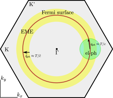
Supplemental Figure S3: A typical scattering event due to the EME interaction in the local approximation, wherethe spin structure factor is assumed to be featureless, i.e., $S(\omega,\bm{q})\approx\rm{const}\times\delta(\omega)$. Starting from $\bm{k}$ (center of green circle) on the Fermi surface (red circle), the local-moments scatter the momentum uniformly throughout the Brillioun zone via the EME term, such that the annulus (yellow) of phonon modes with momenta $\widetilde{q}_{ph}\leq T/\widetilde{c}$ efficiently scatters electrons isotropically on the Fermi surface. In contrast, the conventional el-ph interaction efficiently scatters electrons to a region enclosed by a sphere of radius $q_{ph}\approx T/c$, as shown in the green circle, such that scattering is mainly small-angle up to $\widetilde{T}_{\rm BG}$.

Let us first recall the contribution to the electron-phonon transport scattering time [65, 66] within Boltzmann theory (equivalent to Eq. (2)),

$$\frac{1}{\tau_{\text{el-ph}}}=\frac{4\pi}{\beta}\int_{\Omega}\frac{d\Omega}{\Omega}\alpha^{2}F_{\text{tr}}\left(\Omega\right)\mathcal{K}\left(\beta\Omega\right).$$ (72)

In the Debye approximation for an acoustic mode in 2D, where $\alpha^{2}F_{\text{tr}}\left(\Omega\right)\approx\lambda_{\text{el-ph}}(3/2)\left(\Omega/\Omega_{D}\right)^{3}\theta\left(\Omega_{D}-\Omega\right)$, there is a factor of $\left(\Omega/\Omega_{D}\right)^{2}$ in the el-ph matrix element due to the weighting of small-angle scattering: $1-\cos\left(\theta_{\bm{k},\bm{k^{\prime}}}\right)\sim q^{2}\sim\Omega^{2}$, where $\bm{k},\bm{k^{\prime}}$ are points on the Fermi surface and $\bm{q}$ is the phonon wavevector, see e.g., [8]. In contrast, this weighting is absent in the isotropic EME transport time for reasons highlighted above, which can therefore be approximated as

$$\frac{1}{\tau_{\text{EME}}}=\frac{4\pi}{\beta}\int_{\Omega}\frac{d\Omega}{\Omega}\alpha^{2}F_{\text{EME}}\left(\Omega\right)\mathcal{K}\left(\beta\Omega\right),$$ (73)

where $\alpha^{2}F_{\text{\text{EME}}}\left(\Omega\right)\approx\frac{1}{2}\lambda_{\text{EME}}\left(\Omega/\widetilde{\Omega}_{\text{BG}}\right)\theta\left(\widetilde{\Omega}_{\text{BG}}-\Omega\right)$ (note that $\widetilde{\Omega}_{\rm BG}=\widetilde{T}_{\rm BG}$) and $\mathcal{K}$ defined by Eq. (36). Here we have assumed the BG temperature, rather than the Debye temperature, to be the relevant scale for transport. As described in Fig. S3, the dominant scattering is from thermally excited phonons, which can be seen here by the exponential suppression of $\mathcal{K}(x>1)$. Scattering in this regime if therefore quasi-elastic. In total, we obtain that

$$\frac{1}{\tau_{\text{EME}}}\approx 2\pi\lambda_{\text{EME}}\frac{T^{2}}{\widetilde{T}_{\text{BG}}},\quad J_{\rm H}\ll T\ll\widetilde{T}_{\rm BG},$$ (74)

while for $T\gtrsim\widetilde{T}_{\rm BG}$, $1/\tau_{\text{EME}}\approx 2\pi\lambda_{\text{EME}}T$, as discussed earlier.

References

- Chowdhury et al. [2022] D. Chowdhury, A. Georges, O. Parcollet, and S. Sachdev, Sachdev-Ye-Kitaev models and beyond: Window into non-Fermi liquids, Rev. Mod. Phys. 94, 035004 (2022).
- Varma [2020] C. M. Varma, Colloquium: Linear in temperature resistivity and associated mysteries including high temperature superconductivity, Reviews of Modern Physics 92, 031001 (2020).
- Bruin et al. [2013] J. A. N. Bruin, H. Sakai, R. S. Perry, and A. P. Mackenzie, Similarity of Scattering Rates in Metals Showing T-Linear Resistivity, Science 339, 804 (2013).
- Hartnoll and Mackenzie [2022a] S. A. Hartnoll and A. P. Mackenzie, Colloquium: Planckian dissipation in metals, Reviews of Modern Physics 94, 041002 (2022a).
- Cao et al. [2020] Y. Cao, D. Chowdhury, D. Rodan-Legrain, O. Rubies-Bigorda, K. Watanabe, T. Taniguchi, T. Senthil, and P. Jarillo-Herrero, Strange Metal in Magic-Angle Graphene with near Planckian Dissipation, Physical Review Letters 124, 076801 (2020).
- Legros et al. [2019] A. Legros, S. Benhabib, W. Tabis, F. Laliberté, M. Dion, M. Lizaire, B. Vignolle, D. Vignolles, H. Raffy, Z. Z. Li, P. Auban-Senzier, N. Doiron-Leyraud, P. Fournier, D. Colson, L. Taillefer, and C. Proust, Universal T -linear resistivity and Planckian dissipation in overdoped cuprates, Nature Physics 15, 142 (2019).
- Grissonnanche et al. [2021] G. Grissonnanche, Y. Fang, A. Legros, S. Verret, F. Laliberté, C. Collignon, J. Zhou, D. Graf, P. A. Goddard, L. Taillefer, and B. J. Ramshaw, Linear-in temperature resistivity from an isotropic Planckian scattering rate, Nature 595, 667 (2021).
-
Ziman [1960]
J. M. Ziman, Electrons and Phonons: The
Theory of
Transport Phenomena in Solids, Oxford University Press (1960). - Takagi et al. [1992] H. Takagi, B. Batlogg, H. L. Kao, J. Kwo, R. J. Cava, J. J. Krajewski, and W. F. Peck, Systematic evolution of temperature-dependent resistivity in La2-xSrxCuO4, Physical Review Letters 69, 2975 (1992).
- Hussey et al. [2011] N. E. Hussey, R. A. Cooper, X. Xu, Y. Wang, I. Mouzopoulou, B. Vignolle, and C. Proust, Dichotomy in the T-linear resistivity in hole-doped cuprates, Philosophical Transactions of the Royal Society A: Mathematical, Physical and Engineering Sciences 369, 1626 (2011).
- Doiron-Leyraud et al. [2009] N. Doiron-Leyraud, P. Auban-Senzier, S. René de Cotret, C. Bourbonnais, D. Jérome, K. Bechgaard, and L. Taillefer, Correlation between linear resistivity and in the Bechgaard salts and the pnictide superconductor As2, Phys. Rev. B 80, 214531 (2009).
- Shibauchi et al. [2014] T. Shibauchi, A. Carrington, and Y. Matsuda, A quantum critical point lying beneath the superconducting dome in iron pnictides, Annual Review of Condensed Matter Physics 5, 113 (2014).
- Allen et al. [1996] P. B. Allen, H. Berger, O. Chauvet, L. Forro, T. Jarlborg, A. Junod, B. Revaz, and G. Santi, Transport properties, thermodynamic properties, and electronic structure of , Phys. Rev. B 53, 4393 (1996).
- Klein et al. [1996] L. Klein, J. S. Dodge, C. H. Ahn, G. J. Snyder, T. H. Geballe, M. R. Beasley, and A. Kapitulnik, Anomalous Spin Scattering Effects in the Badly Metallic Itinerant Ferromagnet SrRuO3, Physical Review Letters 77, 2774 (1996).
- Hussey et al. [1998] N. E. Hussey, A. P. Mackenzie, J. R. Cooper, Y. Maeno, S. Nishizaki, and T. Fujita, Normal-state magnetoresistance of Sr2RuO4, Physical Review B 57, 5505 (1998).
- Schneider et al. [2014] M. Schneider, D. Geiger, S. Esser, U. Pracht, C. Stingl, Y. Tokiwa, V. Moshnyaga, I. Sheikin, J. Mravlje, M. Scheffler, and P. Gegenwart, Low-Energy Electronic Properties of Clean CaRuO3: Elusive Landau Quasiparticles, Physical Review Letters 112, 206403 (2014).
- Rost et al. [2011] A. W. Rost, S. A. Grigera, J. A. N. Bruin, R. S. Perry, D. Tian, S. Raghu, S. A. Kivelson, and A. P. Mackenzie, Thermodynamics of phase formation in the quantum critical metal Sr3Ru2O7, Proceedings of the National Academy of Sciences 108, 16549 (2011), https://www.pnas.org/doi/pdf/10.1073/pnas.1112775108 .
- Stewart [2001] G. R. Stewart, Non-Fermi-liquid behavior in - and -electron metals, Reviews of Modern Physics 73, 797 (2001).
- Jaoui et al. [2022] A. Jaoui, I. Das, G. Di Battista, J. Díez-Mérida, X. Lu, K. Watanabe, T. Taniguchi, H. Ishizuka, L. Levitov, and D. K. Efetov, Quantum critical behaviour in magic-angle twisted bilayer graphene, Nature Physics 18, 633 (2022).
- Hwang and Das Sarma [2019] E. H. Hwang and S. Das Sarma, Linear-in- resistivity in dilute metals: A Fermi liquid perspective, Phys. Rev. B 99, 085105 (2019).
- Das Sarma and Wu [2022] S. Das Sarma and F. Wu, Strange metallicity of moiré twisted bilayer graphene, Physical Review Research 4, 033061 (2022).
- Hartnoll and Mackenzie [2022b] S. A. Hartnoll and A. P. Mackenzie, Colloquium: Planckian dissipation in metals, Rev. Mod. Phys. 94, 041002 (2022b).
- Hicks et al. [2015] C. W. Hicks, A. S. Gibbs, L. Zhao, P. Kushwaha, H. Borrmann, A. P. Mackenzie, H. Takatsu, S. Yonezawa, Y. Maeno, and E. A. Yelland, Quantum oscillations and magnetic reconstruction in the delafossite PdCrO2, Phys. Rev. B 92, 014425 (2015).
- Eyert et al. [2008] V. Eyert, R. Frésard, and A. Maignan, On the Metallic Conductivity of the Delafossites PdCoO2 and PtCoO2, Chemistry of Materials 20, 2370 (2008).
- Takatsu et al. [2009] H. Takatsu, H. Yoshizawa, S. Yonezawa, and Y. Maeno, Critical behavior of the metallic triangular-lattice heisenberg antiferromagnet PdCrO2, Physical Review B 79, 104424 (2009).
- Ong et al. [2010] K. P. Ong, J. Zhang, J. S. Tse, and P. Wu, Origin of anisotropy and metallic behavior in delafossite PdCoO2, Physical Review B 81, 115120 (2010).
- Mackenzie [2017] A. P. Mackenzie, The properties of ultrapure delafossite metals, Reports on Progress in Physics 80, 032501 (2017), arXiv:1612.04948 [cond-mat].
- Sunko et al. [2020] V. Sunko, F. Mazzola, S. Kitamura, S. Khim, P. Kushwaha, O. J. Clark, M. D. Watson, I. Marković, D. Biswas, L. Pourovskii, T. K. Kim, T.-L. Lee, P. K. Thakur, H. Rosner, A. Georges, R. Moessner, T. Oka, A. P. Mackenzie, and P. D. C. King, Probing spin correlations using angle-resolved photoemission in a coupled metallic/Mott insulator system, Science Advances 6, eaaz0611 (2020).
- Takatsu et al. [2007a] H. Takatsu, S. Yonezawa, S. Mouri, S. Nakatsuji, K. Tanaka, and Y. Maeno, Roles of High-Frequency Optical Phonons in the Physical Properties of the Conductive Delafossite PdCoO2, Journal of the Physical Society of Japan 76, 104701 (2007a).
- Glamazda et al. [2014] A. Glamazda, W.-J. Lee, S.-H. Do, K.-Y. Choi, P. Lemmens, J. van Tol, J. Jeong, and H.-J. Noh, Collective excitations in the metallic triangular antiferromagnet PdCrO2, Physical Review B 90, 045122 (2014).
- Zhakina et al. [2023] E. Zhakina, R. Daou, A. Maignan, P. H. M. ID, M. König, H. I. Rosner, S.-J. I. Kim, S. I. Khim, R. I. Grasset, M. Konczykowski, E. Tulipman, J. I. F. Mendez-Valderrama, D. I. Chowdhury, E. Berg, and A. P. Mackenzie, Investigation of planckian behavior in a high-conductivity oxide: Pdcro2, Proceedings of the National Academy of Sciences 120, e2307334120 (2023).
- Takatsu et al. [2014] H. Takatsu, G. Nénert, H. Kadowaki, H. Yoshizawa, M. Enderle, S. Yonezawa, Y. Maeno, J. Kim, N. Tsuji, M. Takata, Y. Zhao, M. Green, and C. Broholm, Magnetic structure of the conductive triangular-lattice antiferromagnet PdCrO2, Physical Review B 89, 104408 (2014).
- Daou et al. [2017] R. Daou, R. Frésard, V. Eyert, S. Hébert, and A. Maignan, Unconventional aspects of electronic transport in delafossite oxides, Science and Technology of Advanced Materials 18, 919 (2017).
- Noh et al. [2009] H.-J. Noh, J. Jeong, J. Jeong, E.-J. Cho, S. B. Kim, K. Kim, B. I. Min, and H.-D. Kim, Anisotropic Electric Conductivity of Delafossite PdCoO2 Studied by Angle-Resolved Photoemission Spectroscopy, Physical Review Letters 102, 256404 (2009).
- Noh et al. [2014] H.-J. Noh, J. Jeong, B. Chang, D. Jeong, H. S. Moon, E.-J. Cho, J. M. Ok, J. S. Kim, K. Kim, B. I. Min, H.-K. Lee, J.-Y. Kim, B.-G. Park, H.-D. Kim, and S. Lee, Direct Observation of Localized Spin Antiferromagnetic Transition in PdCrO2 by Angle-Resolved Photoemission Spectroscopy, Scientific Reports 4, 3680 (2014).
- Sunko et al. [2017] V. Sunko, H. Rosner, P. Kushwaha, S. Khim, F. Mazzola, L. Bawden, O. J. Clark, J. M. Riley, D. Kasinathan, M. W. Haverkort, T. K. Kim, M. Hoesch, J. Fujii, I. Vobornik, A. P. Mackenzie, and P. D. C. King, Maximal Rashba-like spin splitting via kinetic-energy-coupled inversion-symmetry breaking, Nature 549, 492 (2017).
- Takatsu and Maeno [2010] H. Takatsu and Y. Maeno, Single crystal growth of the metallic triangular-lattice antiferromagnet PdCrO2, Journal of Crystal Growth 312, 3461 (2010).
- Le et al. [2018] M. D. Le, S. Jeon, A. I. Kolesnikov, D. J. Voneshen, A. S. Gibbs, J. S. Kim, J. Jeong, H.-J. Noh, C. Park, J. Yu, T. G. Perring, and J.-G. Park, Magnetic interactions in PdCrO2 and their effects on its magnetic structure, Physical Review B 98, 024429 (2018).
- [39] See Supplemental Material.
- McRoberts et al. [2023] A. J. McRoberts, J. F. Mendez-Valderrama, R. Moessner, and D. Chowdhury, Intermediate-scale theory for electrons coupled to frustrated local moments, Phys. Rev. B 107, L020402 (2023).
- Keren [1994] A. Keren, Dynamical simulation of spins on kagomé and square lattices, Phys. Rev. Lett. 72, 3254 (1994).
- Moessner and Chalker [1998a] R. Moessner and J. T. Chalker, Properties of a Classical Spin Liquid: The Heisenberg Pyrochlore Antiferromagnet, Phys. Rev. Lett. 80, 2929 (1998a), arXiv:cond-mat/9712063 [cond-mat.stat-mech] .
- Moessner and Chalker [1998b] R. Moessner and J. T. Chalker, Low-temperature properties of classical geometrically frustrated antiferromagnets, Phys. Rev. B 58, 12049 (1998b), arXiv:cond-mat/9807384 [cond-mat.stat-mech] .
- Conlon and Chalker [2009] P. H. Conlon and J. T. Chalker, Spin dynamics in pyrochlore heisenberg antiferromagnets, Phys. Rev. Lett. 102, 237206 (2009).
- Samarakoon et al. [2017] A. M. Samarakoon, A. Banerjee, S. S. Zhang, Y. Kamiya, S. E. Nagler, D. A. Tennant, S. H. Lee, and C. D. Batista, Comprehensive study of the dynamics of a classical Kitaev spin liquid, Phys. Rev. B 96, 134408 (2017), arXiv:1706.10242 [cond-mat.str-el] .
- Bai et al. [2019] X. Bai, J. A. M. Paddison, E. Kapit, S. M. Koohpayeh, J. J. Wen, S. E. Dutton, A. T. Savici, A. I. Kolesnikov, G. E. Granroth, C. L. Broholm, J. T. Chalker, and M. Mourigal, Magnetic Excitations of the Classical Spin Liquid MgCr2 O4, Phys. Rev. Lett. 122, 097201 (2019), arXiv:1810.11869 [cond-mat.str-el] .
- Zhang et al. [2019] S. Zhang, H. J. Changlani, K. W. Plumb, O. Tchernyshyov, and R. Moessner, Dynamical Structure Factor of the Three-Dimensional Quantum Spin Liquid Candidate NaCaNi2F7, Phys. Rev. Lett. 122, 167203 (2019), arXiv:1810.09481 [cond-mat.str-el] .
- Franke et al. [2022] O. Franke, D. Călugăru, A. Nunnenkamp, and J. Knolle, Thermal spin dynamics of Kitaev magnets – scattering continua and magnetic field induced phases within a stochastic semiclassical approach, arXiv e-prints , arXiv:2207.03515 (2022), arXiv:2207.03515 [cond-mat.str-el] .
- Kennes et al. [2021] D. M. Kennes, M. Claassen, L. Xian, A. Georges, A. J. Millis, J. Hone, C. R. Dean, D. N. Basov, A. N. Pasupathy, and A. Rubio, Moiré heterostructures as a condensed-matter quantum simulator, Nature Physics 17, 155 (2021).
- Mak and Shan [2022] K. F. Mak and J. Shan, Semiconductor moiré materials, Nature Nanotechnology 10.1038/s41565-022-01165-6 (2022).
- Li et al. [2021] T. Li, S. Jiang, L. Li, Y. Zhang, K. Kang, J. Zhu, K. Watanabe, T. Taniguchi, D. Chowdhury, L. Fu, J. Shan, and K. F. Mak, Continuous Mott transition in semiconductor moiré superlattices, Nature 597, 350 (2021).
- Ghiotto et al. [2021] A. Ghiotto, E.-M. Shih, G. S. S. G. Pereira, D. A. Rhodes, B. Kim, J. Zang, A. J. Millis, K. Watanabe, T. Taniguchi, J. C. Hone, L. Wang, C. R. Dean, and A. N. Pasupathy, Quantum criticality in twisted transition metal dichalcogenides, Nature 597, 345 (2021).
- Kumar et al. [2022] A. Kumar, N. C. Hu, A. H. MacDonald, and A. C. Potter, Gate-tunable heavy fermion quantum criticality in a moiré Kondo lattice, Phys. Rev. B 106, L041116 (2022).
- Dalal and Ruhman [2021] A. Dalal and J. Ruhman, Orbitally selective mott phase in electron-doped twisted transition metal-dichalcogenides: A possible realization of the Kondo lattice model, Phys. Rev. Research 3, 043173 (2021).
- Zhao et al. [2022] W. Zhao, B. Shen, Z. Tao, Z. Han, K. Kang, K. Watanabe, T. Taniguchi, K. F. Mak, and J. Shan, Gate-tunable heavy fermions in a moiré Kondo lattice, arXiv e-prints , arXiv:2211.00263 (2022), arXiv:2211.00263 [cond-mat.str-el] .
- Vavno et al. [2021] V. Vavno, M. Amini, S. C. Ganguli, G. Chen, J. L. Lado, S. Kezilebieke, and P. Liljeroth, Artificial heavy fermions in a van der waals heterostructure, Nature 599, 582 (2021).
- Persky et al. [2022] E. Persky, A. V. Bjørlig, I. Feldman, A. Almoalem, E. Altman, E. Berg, I. Kimchi, J. Ruhman, A. Kanigel, and B. Kalisky, Magnetic memory and spontaneous vortices in a van der waals superconductor, Nature 607, 692 (2022).
- Hicks et al. [2012] C. W. Hicks, A. S. Gibbs, A. P. Mackenzie, H. Takatsu, Y. Maeno, and E. A. Yelland, Quantum oscillations and high carrier mobility in the delafossite PdCoO2, Phys. Rev. Lett. 109, 116401 (2012).
- Takatsu et al. [2007b] H. Takatsu, S. Yonezawa, S. Mouri, S. Nakatsuji, K. Tanaka, and Y. Maeno, Roles of High-Frequency Optical Phonons in the Physical Properties of the Conductive Delafossite PdCoO2, Journal of the Physical Society of Japan 76, 104701 (2007b), https://doi.org/10.1143/JPSJ.76.104701 .
- Takatsu et al. [2010] H. Takatsu, S. Yonezawa, C. Michioka, K. Yoshimura, and Y. Maeno, Anisotropy in the magnetization and resistivity of the metallic triangular-lattice magnet pdcro2, Journal of Physics: Conference Series 200, 012198 (2010).
- Ghannadzadeh et al. [2017] S. Ghannadzadeh, S. Licciardello, S. Arsenijević, P. Robinson, H. Takatsu, M. I. Katsnelson, and N. E. Hussey, Simultaneous loss of interlayer coherence and long-range magnetism in quasi-two-dimensional pdcro2, Nature Communications 8, 15001 (2017).
- Putzke et al. [2020] C. Putzke, M. D. Bachmann, P. McGuinness, E. Zhakina, V. Sunko, M. Konczykowski, T. Oka, R. Moessner, A. Stern, M. König, S. Khim, A. P. Mackenzie, and P. J. Moll, oscillations in interlayer transport of delafossites, Science 368, 1234 (2020), https://www.science.org/doi/pdf/10.1126/science.aay8413 .
- Kohn [1959] W. Kohn, Image of the Fermi surface in the vibration spectrum of a metal, Phys. Rev. Lett. 2, 393 (1959).
- Sunko [2019] V. Sunko, Angle Resolved Photoemission Spectroscopy of Delafossite Metals (2019).
- Allen and Schulz [1993] P. B. Allen and W. W. Schulz, Bloch-boltzmann analysis of electrical transport in intermetallic compounds: ReO3, BaPbO3, CoSi2, and Pd2Si, Phys. Rev. B 47, 14434 (1993).
- Sadovskii [2019] M. V. Sadovskii, Diagrammatics: Lectures on Selected Problems in Condensed Matter Theory (2019).
SUPPLEMENTARY INFORMATION