Range-controlled random walks

Abstract

We introduce range-controlled random walks with hopping rates depending on the range $\mathcal{N}$, that is, the total number of previously distinct visited sites. We analyze a one-parameter class of models with a hopping rate $\mathcal{N}^{a}$ and determine the large time behavior of the average range, as well as its complete distribution in two limit cases. We find that the behavior drastically changes depending on whether the exponent $a$ is smaller, equal, or larger than the critical value, $a_{d}$, depending only on the spatial dimension $d$. When $a>a_{d}$, the forager covers the infinite lattice in a finite time. The critical exponent is $a_{1}=2$ and $a_{d}=1$ when $d\geq 2$. We also consider the case of two foragers who compete for food, with hopping rates depending on the number of sites each visited before the other. Surprising behaviors occur in 1d where a single walker dominates and finds most of the sites when $a>1$, while for $a<1$, the walkers evenly explore the line. We compute the gain of efficiency in visiting sites by adding one walker.

The range $\mathcal{N}(t)$, that is, the number of distinct sites visited at time $t$, is a central observable of the random walk theory. This quantity has been the subject of a large number of works in various fields, ranging from physics and chemistry to ecology Weiss and Rubin (1983); Hughes (1996); Weiss (1994); Redner (2001). A key result is that the average range of the symmetric nearest-neighbor random walk exhibits the following asymptotic behaviors 

$$N(t)\equiv\langle\mathcal{N}(t)\rangle\sim\begin{cases}\sqrt{\frac{8ht}{\pi}}&d=1\\ \frac{\pi ht}{\ln ht}&d=2\\ ht/W_{d}&d>2\end{cases}$$ (1)

where $W_{d}$ are Watson integrals Watson (1939); Glasser and Zucker (1977); Guttmann (2010); Zucker (2011) and $h$ the constant hopping rate . The sublinear behavior in $d\leq 2$ dimensions is a direct consequence of the recurrence of random walks in low dimensions. Beyond the average, the ratio $\sqrt{\text{Var}[\mathcal{N}(t)]}/N(t)$ is known to go to 0 in the large time limit when $d\geq 2$; it remains finite for $d=1$. Thus the range $\mathcal{N}(t)$ is asymptotically self-averaging random quantity when $d\geq 2$, namely its distribution is asymptotically a Dirac delta function peaked at the average value. In 1d, the range is a non-self-averaging random quantity.

In addition to its central place in random walk theory, the range has proven to be a fundamental tool to quantify the efficiency of random explorations, as it is the case in foraging theory Larralde et al. (1992a, b); Viswanathan et al. (1999, 2011); Ben-Avraham and Havlin (2000); Bénichou et al. (2005, 2011). The minimal models involve a forager, described as a RW, that gradually depletes the resource contained in a medium as it moves. The medium is a $d$-dimensional lattice with a food unit at each site at $t=0$. When the walker encounters a site containing food, it consumes it so that the amount of food collected at time $t$ is the range $\mathcal{N}(t)$. This class of models accounts for the depletion of food induced by the motion of the forager, yet the movement of the walker is not affected by the consumption of resources. Depending on the situation, the food collected along the path can provide additional energy to search for food or, because it represents extra weight, to slow down the walk. As a result, there is a clear coupling between the range $\mathcal{N}(t)$ and the dynamical properties of the RW. No modeling of this effect has been proposed so far, even at a schematic level.

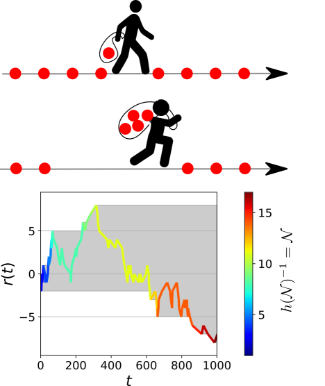
Figure 1: Representation of a walker penalized upon acquiring new targets. Top: Representation of the random walk slowed down by the load collected on distinct visited sites. Bottom: Trajectory of a symmetric $1d$ nearest neighbor random walk in the particular case of hopping rates $h(\mathcal{N})$ varying as the inverse of the number of distinct sites visited, $\mathcal{N}^{-1}$. The grey area corresponds to the explored territory, and the coloring refers to the number of distinct sites visited.

Here, we fill this gap and introduce range-controlled random walks as a model accounting for this coupling, for which the hopping rate is a monotonic function $h(\mathcal{N})$ of the range, either increasing or decreasing (see Fig. 1). For concreteness, we consider the case where the hopping rate is a power of the amount of collected food: $h(\mathcal{N})=\mathcal{N}^{a}$. However, our results still apply when this algebraic dependence holds only asymptotically when $\mathcal{N}\gg 1$. In the context of search problems Bénichou et al. (2011), models with positive [resp. negative] exponent $a$ mimic the walker rewarded [resp. penalized] and accelerated [resp. decelerated] upon acquiring new targets (see Fig. 1). Because the coupling between the range and the dynamical properties of foragers is natural and because our modeling of this coupling is minimal, the model of range-controlled random walks quantifies the efficiency of foraging and appears relevant at broader scale to random explorations.

At the theoretical level, range-controlled random walks belong to the class of non-Markovian random walks, in which the memory of trajectory or some of its features influences the choice of destination sites. Representative examples comprise self-avoiding walks Rudnick and Gaspari (2004); Madras and Slade (2013), true self-avoiding walkers Amit et al. (1983); Pietronero (1983); Obukhov and Peliti (1983); Peliti and Pietronero (1987); Grassberger (2017), self-interacting random walks Perman and Werner (1997); Davis (1999); Pemantle and Volkov (1999); Dickman and ben Avraham (2001); Benjamini and Wilson (2003); Zerner (2005); Antal and Redner (2005); Kosygina and Zerner (2013); Boyer and Solis-Salas (2014); Campos and Méndez (2019); Barbier-Chebbah et al. (2020, 2022) and random walks with reinforcement such as the elephant walks Schütz and Trimper (2004); Paraan and Esguerra (2006); Baur and Bertoin (2016); Bercu and Laulin (2021); Bertoin (2022). In all of these models, the total hopping rate is kept constant . Determining the range of non-Markovian random walks is notoriously difficult, and very few exact results are available.

Beyond this theoretical challenge, non-Markovian random walks with memory emerging from the interaction of the walker with the territory already visited are relevant in the case of living cells Mierke (2021); Mierke et al. (2010); Mierke (2014); Charras and Sahai (2014); Mierke (2019). It has indeed been observed in vitro D’alessandro et al. (2021); Flyvbjerg (2021), both in 1d and 2d situations, that various cell types can chemically modify the extracellular matrix, which in turn deeply impact their motility. In this context, range-controlled random walks appears as a minimal model where the modifications induced by the passage of cells are described in a mean-field way: all the complexity of the “perturbation”, be it the concentration field of nutrients Macklin and Lowengrub (2007), the local orientation of matrix fibers Schlüter et al. (2012) or hydrodynamics fields Heck et al. (2017) is assumed to be encapsulated in the extension of the domain visited by the cell (i.e., the range of the associated random-walk). It is then natural to mimic the “response” of the cell by a modification of a dynamical parameter, and we finally end up with a hopping rate $h(\mathcal{N})$ depending on the range as introduced above.

Summary of the Results. In this Letter, we quantify the efficiency of $d$-dimensional range-controlled random walks by determining exact asymptotic expressions of their average range, as well as the full distribution in $d=1$ and in the $d\to\infty$ limit. This allows us to unveil a surprising transition and show that the behavior of range-controlled random walks drastically changes depending on whether the exponent $a$ is smaller, equal, or larger than the critical value, $a_{d}$, depending only on the spatial dimension: $a_{1}=2$ in $d=1$ and $a_{d}=1$ when $d\geq 2$. The explosive behavior occurs in the supercritical $a>a_{d}$ regime: The forager covers the entire infinite lattice in a finite time.

The behavior in the $a\leq a_{d}$ regime can be appreciated from the growth of the average number $N(t)$ of distinct visited sites. When $a<a_{d}$, the growth is algebraic with a logarithmic correction in 2d:

$$N(t)\sim C_{d}(a)\times\begin{cases}t^{\frac{1}{2-a}}&d=1\\ \left(\frac{t}{\ln t}\right)^{\frac{1}{1-a}}&d=2\\ t^{\frac{1}{1-a}}&d>2\end{cases}$$ (2)

The amplitudes are

$$C_{1}(a) =\frac{2^{1+\frac{1}{2-a}}}{\Gamma\left(\frac{1}{2-a}\right)}\int_{0}^{\infty}\frac{dv}{v}\left[\frac{\sqrt{v}}{\cosh v}\right]^{\frac{4}{2-a}},\quad a<2$$ (3a)

$$C_{2}(a) =\left[\pi(1-a)^{2}\right]^{\frac{1}{1-a}},\quad a<1$$ (3b)

$$C_{d}(a) =\left(\frac{1-a}{W_{d}}\right)^{\frac{1}{1-a}},\qquad a<1,\qquad d\geq 3\;.$$ (3c)

In the critical regime $a=a_{d}$, the growth is exponential

$$\ln N(t)\sim\begin{cases}\lambda_{1}t&d=1,~{}~{}a=2\\ \lambda_{2}\sqrt{t}&d=2,~{}~{}a=1\\ \lambda_{d}t&d>2,~{}~{}a=1\end{cases}$$ (4)

with growth rates

$$\lambda_{1}=1,\quad\lambda_{2}=\sqrt{2\pi}\,,\quad\lambda_{d}=1/W_{d}\quad(d>2)\;.$$ (5)

We discuss the competition between two foragers by determining the average number of distinct sites $N_{2}(t)$ visited by two foragers in $1d$ where their respective hopping rate depends on the number of distinct sites the walker visited before the other. In particular, by defining $N_{1}(t)$ as the average number of distinct sites visited by a single walker (without any other walker), we get an analytical value for the ratio at large times:

$$\lim_{t\to\infty}\frac{N_{2}(t)}{N_{1}(t)}=r_{2}(a)=\begin{cases}2^{\frac{1-a}{2-a}}&a<1\\ 1&a>1\;.\end{cases}$$ (6)

This ratio quantifies the efficiency gain in finding new sites by adding one RW. In particular, we observe that for foragers accelerating fast enough with the number of distinct sites visited $(a>1)$, there is no gain in adding the second walker.

1d. Let $P_{n}(t)\equiv\mathbf{P}(\mathcal{N}(t)=n)$ be the range distribution and $\Pi_{n}(t)\equiv\mathbf{P}(\mathcal{N}(t)\geq n)$ the corresponding complementary cumulative distribution. In the 1d situation, an exact expression for the entire distribution of the range can be obtained. This exact solution relies on the observation that (see Régnier et al. (2022, 2023))

$$\{\mathcal{N}(t)\geqslant n\} = \left\{\sum\limits_{k=1}^{n-1}\tau_{k}\leqslant t\right\}$$ (7)

where $\tau_{k}$ is the time elapsed between the visit of the $k^{\text{th}}$ and $(k+1)^{\text{st}}$ site by the RW defined above. The key points are that (i) during this exploration, the walker has a constant hopping rate, $k^{a}$, and (ii) the $\tau_{k}$’s are independent random variables. Performing the Laplace transform ($\widehat{f}(s)\equiv\int_{0}^{\infty}f(t)e^{-st}dt$) of the probability of these events we get

$$\widehat{\Pi}_{n}(s) = \frac{1}{s}\prod_{k=1}^{n-1}\widehat{F}_{k}(s)$$ (8)

where $\widehat{F}_{k}$ is the Laplace transform of the distribution of the random variable $\tau_{k}$. Here $\tau_{k}$ is the exit time from an interval of $k$ sites starting on the boundary. At small $s$ (corresponding to large time), $\widehat{F}_{k}$ is given by the exit time distribution of an interval of length $k+1$ starting at distance one of the border of a continuous Brownian motion with diffusion constant $D_{k}\equiv\frac{1}{2}k^{a}$ Redner (2001),

$$\widehat{F}_{k}(s) = \frac{\sinh\left(\sqrt{\frac{s}{D_{k}}}k\right)+\sinh\left(\sqrt{\frac{s}{D_{k}}}\right)}{\sinh\left(\sqrt{\frac{s}{D_{k}}}(k+1)\right)}\;.$$ (9)

This expression involves $k/\sqrt{D_{k}}\propto k^{1-a/2}$, and reveals the existence of three different regimes.

(i) In the subcritical regime $a<a_{c}=2$, taking the limit $k\to\infty$ and $s\to 0$ while keeping $k^{2-a}s$ finite, gives

$$\widehat{F}_{k}(s)-1\sim-\sqrt{2s}k^{-a/2}\tanh\left(\sqrt{\frac{s}{2}}k^{1-a/2}\right)$$ (10)

and then (see Supplementary Material, SM, S1 and S2)

$$\widehat{P}_{n}(s) =\widehat{\Pi}_{n}(s)-\widehat{\Pi}_{n+1}(s)$$

$$\sim-\partial_{n}\widehat{\Pi}_{n}(s)$$

$$\sim-\partial_{n}\left(\frac{1}{s\cosh\left(n^{1-a/2}s^{1/2}/\sqrt{2}\right)^{\frac{4}{2-a}}}\right)\;.$$ (11)

In particular, for $a=0$, we recover the well-known range distribution Hughes (1996) for a standard random walk. One can extract the average range, viz. Eqs. (2) and (3a), from the small $s$ asymptotic. In addition, $P_{n}(t)$ acquires a scaling form $P_{n}(t)=t^{-\frac{1}{2-a}}\phi_{a}(x)$ ($x=n/t^{\frac{1}{2-a}}$), where $\phi_{a}$ is a function of the scaling variable $x$ depending on the exponent $a$. Explicit analytical expressions are provided and displayed in SM for accelerated and slowed down foragers.

(ii) In the critical regime, $a=a_{c}=2$ in 1d, $\widehat{F}_{k}(s)-1\sim-s/k$ and $P_{n}(t)\sim\delta\left(n-e^{t}\right)$ (see SM). Thus $\mathcal{N}(t)$ is asymptotically deterministic, chiefly characterized by exponentially growing average $e^{\lambda_{1}t}$ with $\lambda_{1}=1$ as stated in Eq. (5).

(iii) In the supercritical regime, $a>a_{c}=2$, the dynamics is explosive, and the entire infinite lattice is covered in a finite time (see SM).

Higher dimensions. In the $d\to\infty$ limit, the entire distribution of the range can also be obtained (see SM). In this case, the average $N$ and the variance $V$ of the number of distinct visited sites exhibit asymptotically identical growth:

$$N\sim[(1-a)t]^{\frac{1}{1-a}}\sim V$$ (12)

This shows the self-averaging nature of $\mathcal{N}$ in the sub-critical regime (for $d\to\infty$) as the standard deviation is negligible compared to the average.
For finite dimensions, when $a\leq a_{d}$, the asymptotic behavior of the average range can be obtained from heuristic arguments. In the case of varying hopping rates, we use (1) and a self-consistent estimate $h=N^{a}$ of the typical hopping rate. In 1d, for instance, this leads to $N\propto\sqrt{N^{a}t}$, from which $N\propto t^{\frac{1}{2-a}}$, in agreement with the exact solution provided in Eq. (2). Similarly we arrive at the announced growth laws (2) in higher dimensions. These results show that $a_{d}=1$ when $d\geq 2$. We now turn to the determination of the amplitudes $C_{d}(a)$ (for $a<a_{d}$) and the growth rates $\lambda_{d}$ (for $a=a_{d}$).

In $d>2$ dimensions, the proper interpretation of (1) is that a RW hops to unvisited sites with probability that approaches $1/W_{d}$ Hughes (1996). Thus

$$N(t)\sim(W_{d})^{-1}H(t)$$ (13)

where $H$ is the average total number of hops. Using

$$H(t)\sim\int_{0}^{t}d\tau\,[N(\tau)]^{a}\sim(1-a)[C_{d}(a)]^{a}t^{\frac{1}{1-a}}$$ (14)

we arrive at $C_{d}(a)=(1-a)[C_{d}(a)]^{a}/W_{d}$ leading to the announced result (3c).

The relation (13) is asymptotically exact, but averaging the total number of hops

$$\mathcal{H}=\int_{0}^{t}d\tau\,[\mathcal{N}(\tau)]^{a}$$ (15)

gives (14) only if $\langle\mathcal{N}^{a}\rangle=\langle\mathcal{N}\rangle^{a}$. This is erroneous (when $a\neq 1$) if the random quantity $\mathcal{N}$ is non-self-averaging as it is in 1d. Since $\mathcal{N}$ is self-averaging if $d\geq 2$, the prediction (3c) is exact (see also the agreement with numerical simulations displayed in Fig. 2). In the critical regime, $a=1$, we have $\dot{H}=N$ which we insert into (13) and obtain the differential equation $\dot{H}=H/W_{d}$, whose solution is $H\propto e^{t/W_{d}}$. The range is also exponential confirming (4) and (5) for $d>2$.

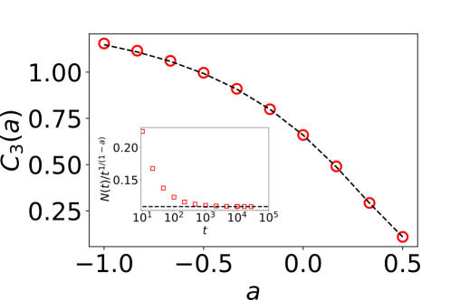
Figure 2: Comparison of the coefficient $C_{3}(a)$ obtained in (3c) (black dashed line) and the results of numerical simulations (red circles) obtained by evaluating $\lim\limits_{t\to\infty}\frac{N(t)}{t^{1/(1-a)}}$. The subfigure represents $N(t)/t^{1/(1-a)}$ (red squares) for increasing values of $t$ in the particular case $a=1/2$. It shows the convergence to $C_{3}(a)$ (black dashed line).

In 2d, the exact asymptotic in (1) implies $N\sim\pi H/\ln H$. When $a<1$, taking $h=N^{a}$ in Eq. (1) in the $2d$ case, we obtain $N\propto\frac{N^{a}t}{\ln N^{a}t}$ and $N\propto\left(\frac{t}{\ln t}\right)^{\frac{1}{1-a}}$. We note the constant prefactor $C_{2}(a)$, as defined in (2). Then similarly to Eq. (14),

$$H \sim \int_{0}^{t}d\tau\,[N(\tau)]^{a}$$ (16)

$$\sim (1-a)[C_{2}(a)]^{a}\,t^{\frac{1}{1-a}}(\ln t)^{-\frac{a}{1-a}}\;.$$

Equating $N$ to

$$\frac{\pi H}{\ln H}\sim\pi(1-a)^{2}[C_{2}(a)]^{a}\,(t/\ln t)^{\frac{1}{1-a}}$$

fixes the amplitude and yields the announced result (3b). In the critical $a=1$ regime, the growth is stretched exponential in 2d (see (4)). Indeed, $H(t)$ asymptotically satisfies $\dot{H}=\frac{\pi H}{\ln H}$, whose solution is $H\propto e^{\sqrt{2\pi t}}$. This confirms (4) with $\lambda_{2}=\sqrt{2\pi}$ in 2d. Thus we have established (4) and (5) in all dimensions (see SM Fig. 3 for the comparison with numerical simulations).

Two foragers. We now discuss the competition of foragers. The forager with label $j$ has the hopping rate $\mathcal{F}_{j}^{a}$, where $\mathcal{F}_{j}$ is the number of sites first visited by the forager. For one forager, $\mathcal{F}_{1}=\mathcal{N}_{1}$ is just the range. For two foragers, $\mathcal{F}_{1}+\mathcal{F}_{2}=\mathcal{N}_{2}$ is the total range. Foragers do not directly interact, but their motion changes the environment that, in turn, affects the motion of the foragers.

To compare the two-foragers and the single-forager cases, we consider the ratio $N_{2}/N_{1}$ of the average numbers of distinct visited sites in both settings. The ratio $r_{2}(a)$ defined in Eq. (6) depends only on the exponent $a$ and is non-trivial only in 1d, as $r_{2}(a)=2$ for $d\geq 2$ as a consequence of Ben-Naim and Krapivsky (2022), the number of common sites visited by the two RWs being asymptotically negligible compared to the number of distinct sites visited by each one of them in this case. Hereinafter we consider foraging in 1d in the non-explosive regime, $a\leq 2$. For 1d RWs, the ratio $r_{2}(0)=\sqrt{2}$ is smaller than 2 reflecting the severe space limitation in 1d (see SM).

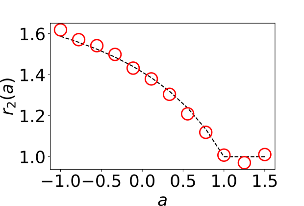
Figure 3: Comparison of the theoretical prediction of the ratio $r_{2}(a)=\max\left(1,2^{\frac{1-a}{2-a}}\right)$ (black dashed lines) and numerical simulation $\lim\limits_{t\to\infty}\frac{N_{2}(t)}{N_{1}(t)}$ (red circles, whose diameters correspond to the largest error bar estimation) of the average number of distinct sites visited by two foragers, $N_{2}(t)$, versus the average number of distinct sites visited by a single one, $N_{1}(t)$.

One has to differentiate between two regimes, $a<1$ and $a>1$. When $a<1$, both foragers visit the 1d lattice equally (on average). Thus the rate of finding new sites is known by solving the problem at $a=0$. Using a proper rescaling of the times by $(N_{2}/2)^{a}$ corresponding to the hopping rate of one of the forager (similarly to what we did with (1)), one establishes (6). When $a>1$, the hypothesis that sites are equally visited breaks down. To understand the transition, suppose one walker ($W_{1}$) has found $k\gg 1$ sites, while he other ($W_{2}$) has found $\ell\ll k$ sites. If $W_{2}$ finds a new site at some time $t\gg 1$, which walker will be first to find a new site? The walker $W_{2}$ will find a new site in a typical time $\propto k/\ell^{a}$, as it is positioned at the border of the interval of at most $k+\ell\approx k$ distinct sites visited by $W_{1}$ and $W_{2}$. The position of $W_{1}$ is unknown, effectively uniform in the interval of $k$ distinct sites visited, but it hops much faster than $W_{2}$ and so the average time of finding a new site is $k^{2}/k^{a}=k^{2-a}$. Thus, if $a>1$, even though it is further away from the border than $W_{2}$, the walker $W_{1}$ will be the first to find a new site ($k^{2-a}\ll k/\ell^{a}$). This situation is stable if $a>1$ (the dominant walker with the most distinct visited sites will become more and more dominating) and unstable if $a<1$ (the subdominant walker catches up). The theoretical prediction is validated by numerical simulations (Fig. 3).

We introduced random walks with range-dependent hopping rates behaving as $\mathcal{N}^{a}$ when $\mathcal{N}\gg 1$. Our analysis provides the exact full distribution of the range in 1d, and also on a complete graph mimicking an infinite-dimensional setting. For a random walk on a hyper-cubic lattice $\mathbb{Z}^{d}$ with $d\geq 2$, we used a heuristic approach relying on results for the classical random walk ($a=0$). We argued that this argument gives asymptotically exact results for the average range when $d\geq 2$. The above sub-critical behaviors occur when $a<a_{d}$ with $a_{1}=2$ and $a_{d}=1$ when $d\geq 2$. When $a>a_{d}$, the entire infinite lattice $\mathbb{Z}^{d}$ is covered in a finite time.

References

- Weiss and Rubin (1983) G. H. Weiss and R. J. Rubin, in Adv. Chem. Phys., Vol. 52, edited by I. Prigogine and S. A. Rice (Wiley-Interscience, 1983) pp. 363–505.
- Hughes (1996) B. Hughes, Random Walks and Random Environments, Vol. 1: Random Walks, Oxford science publications (Clarendon Press, 1996).
- Weiss (1994) G. H. Weiss, Aspects and Applications of the Random Walk (North-Holland, Amsterdam, 1994).
- Redner (2001) S. Redner, A Guide to First-Passage Processes (Cambridge University Press, Cambridge, UK, 2001).
- Note (1) We consider hyper-cubic lattices, so e.g. the prediction of (1) in 2d refers to the square grid.
- Watson (1939) G. N. Watson, Quart. J. Math. Oxford 10, 266 (1939).
- Glasser and Zucker (1977) M. L. Glasser and I. J. Zucker, Proc. Natl. Acad. Sci. U.S.A. 74, 1800 (1977).
- Guttmann (2010) A. J. Guttmann, J. Phys. A 43, 305205 (2010).
- Zucker (2011) I. J. Zucker, J. Stat. Phys. 145, 591 (2011).
- Note (2) The hopping rate is where is the lattice coordination number and the diffusion coefficient of the random walker (RW). Hence for the RW on the hyper-cubic lattice .
- Larralde et al. (1992a) H. Larralde, P. Trunfio, H. E. Stanley, and G. H. Weiss, Nature 355, 423 (1992a).
- Larralde et al. (1992b) H. Larralde, P. Trunfio, S. Havlin, H. E. Stanley, and G. H. Weiss, Phys. Rev. A 45, 7128 (1992b).
- Viswanathan et al. (1999) G. Viswanathan, S. V. Buldyrev, S. Havlin, M. G. E. da Luz, E. P. Raposo, and H. E. Stanley, Nature 401, 911 (1999).
- Viswanathan et al. (2011) G. M. Viswanathan, M. G. D. Luz, E. P. Raposo, and H. E. Stanley, The physics of foraging: an introduction to random searches and biological encounters (Cambridge University Press, Cambridge, UK, 2011).
- Ben-Avraham and Havlin (2000) D. Ben-Avraham and S. Havlin, Diffusion and reactions in fractals and disordered systems (Cambridge University Press, Cambridge, UK, 2000).
- Bénichou et al. (2005) O. Bénichou, M. Coppey, M. Moreau, P. H. Suet, and R. Voituriez, J. Phys.: Condens. Matter 17, S4275 (2005).
- Bénichou et al. (2011) O. Bénichou, C. Loverdo, M. Moreau, and R. Voituriez, Rev. Mod. Phys. 83, 81 (2011).
- Rudnick and Gaspari (2004) J. Rudnick and G. Gaspari, Elements of the Random Walk: An Introduction for Advanced Students and Researchers (Cambridge University Press, Cambridge, New York, 2004).
- Madras and Slade (2013) N. Madras and G. Slade, The Self-Avoiding Walk (Birkhäuser, New York, NY, 2013).
- Amit et al. (1983) D. J. Amit, G. Parisi, and L. Peliti, Phys. Rev. B 27, 1635 (1983).
- Pietronero (1983) L. Pietronero, Phys. Rev. B 27, 5887 (1983).
- Obukhov and Peliti (1983) S. P. Obukhov and L. Peliti, J. Phys. A 16, L147 (1983).
- Peliti and Pietronero (1987) L. Peliti and L. Pietronero, Riv. Nuovo Cim 10, 1 (1987).
- Grassberger (2017) P. Grassberger, Phys. Rev. Lett. 119, 140601 (2017).
- Perman and Werner (1997) M. Perman and W. Werner, Probab. Theory Related Fields 108, 357 (1997).
- Davis (1999) B. Davis, Probab. Theory Relat. Fields 1, 501 (1999).
- Pemantle and Volkov (1999) P. Pemantle and S. Volkov, Ann. Probab. 27, 1368 (1999).
- Dickman and ben Avraham (2001) R. Dickman and D. ben Avraham, Phys. Rev. E 64, 020102 (2001).
- Benjamini and Wilson (2003) I. Benjamini and D. Wilson, Electron. Commun. Probab. 8, 86 (2003).
- Zerner (2005) M. P. W. Zerner, Probab. Theory Relat. Fields 133, 98 (2005).
- Antal and Redner (2005) T. Antal and S. Redner, J. Phys. A 38, 2555 (2005).
- Kosygina and Zerner (2013) E. Kosygina and M. P. W. Zerner, Bull. Inst. Math. Acad. Sin. (New Series) 8, 105 (2013).
- Boyer and Solis-Salas (2014) D. Boyer and C. Solis-Salas, Phys. Rev. Lett. 112, 240601 (2014).
- Campos and Méndez (2019) D. Campos and V. Méndez, Phys. Rev. E 99, 062137 (2019).
- Barbier-Chebbah et al. (2020) A. Barbier-Chebbah, O. Benichou, and R. Voituriez, Phys. Rev. E 102, 062115 (2020).
- Barbier-Chebbah et al. (2022) A. Barbier-Chebbah, O. Bénichou, and R. Voituriez, Phys. Rev. X 12, 011052 (2022).
- Schütz and Trimper (2004) G. M. Schütz and S. Trimper, Phys. Rev. E 70, 045101 (2004).
- Paraan and Esguerra (2006) F. N. C. Paraan and J. P. Esguerra, Phys. Rev. E 74, 032101 (2006).
- Baur and Bertoin (2016) E. Baur and J. Bertoin, Phys. Rev. E 94, 052134 (2016).
- Bercu and Laulin (2021) B. Bercu and L. Laulin, Stoch. Processes Appl. 133, 111 (2021).
- Bertoin (2022) J. Bertoin, Trans. Amer. Math. Soc. 375, 1 (2022).
- Note (3) Notable exceptions are the locally activated random walk model Bénichou et al. (2012), where the hopping rate depends on the number of visits of a specific site, and the accelerated cover problem Maziya et al. (2020), where the hopping rate is a function of the typical time to visit a new site.
- Mierke (2021) C. T. Mierke, Frontiers in Physics 9, 749830 (2021).
- Mierke et al. (2010) C. T. Mierke, P. Kollmannsberger, D. P. Zitterbart, G. Diez, T. M. Koch, S. Marg, W. H. Ziegler, W. H. Goldmann, and B. Fabry, Journal of Biological Chemistry 285, 13121 (2010).
- Mierke (2014) C. T. Mierke, Reports on Progress in Physics 77, 076602 (2014).
- Charras and Sahai (2014) G. Charras and E. Sahai, Nature reviews Molecular cell biology 15, 813 (2014).
- Mierke (2019) C. T. Mierke, Reports on Progress in Physics 82, 064602 (2019).
- D’alessandro et al. (2021) J. D’alessandro, A. Barbier-Chebbah, V. Cellerin, O. Benichou, R. M. Mège, R. Voituriez, and B. Ladoux, Nature Communications 12, 4118 (2021).
- Flyvbjerg (2021) H. Flyvbjerg, Nature Physics 17, 771 (2021).
- Macklin and Lowengrub (2007) P. Macklin and J. Lowengrub, Journal of Theoretical Biology 245, 677–704 (2007).
- Schlüter et al. (2012) D. K. Schlüter, I. Ramis-Conde, and M. A. Chaplain, Biophysical Journal 103, 1141–1151 (2012).
- Heck et al. (2017) T. Heck, B. Smeets, S. Vanmaercke, P. Bhattacharya, T. Odenthal, H. Ramon, H. V. Oosterwyck, and P. V. Liedekerke, Computer Methods in Applied Mechanics and Engineering 322, 515–540 (2017).
- Régnier et al. (2022) L. Régnier, M. Dolgushev, S. Redner, and O. Bénichou, Phys. Rev. E 105, 064104 (2022).
- Régnier et al. (2023) L. Régnier, M. Dolgushev, S. Redner, and O. Bénichou, Nature Communications 14, 618 (2023).
- Ben-Naim and Krapivsky (2022) E. Ben-Naim and P. L. Krapivsky, J. Stat. Mech. 2022, 103208 (2022).
- Bénichou et al. (2012) O. Bénichou, N. Meunier, S. Redner, and R. Voituriez, Phys. Rev. E 85, 021137 (2012).
- Maziya et al. (2020) G. Maziya, L. Cocconi, G. Pruessner, and N. R. Moloney, Phys. Rev. Res. 2, 023421 (2020).