1 Introduction

The QCD axion and axion-like particles (ALPs), collectively referred to as axions, are intriguing candidates for light dark matter (DM) [1, 2, 3] (see Refs. [4, 5, 6, 7, 8, 9, 10] for reviews). The axion is a pseudo Nambu-Goldstone boson associated with the spontaneously broken Peccei-Quinn (PQ) symmetry  [11, 12, 13, 14], which is anomalous under the standard model (SM) gauge groups. Axion models are frequently explored in the context of grand unified theory (GUT), which accounts for the charge quantization of SM particle contents (see, for example, recent studies of the QCD axion and GUT in Refs. [15, 16, 17, 18, 19]). In fact, known quarks and leptons are neatly embedded in complete GUT multiplets. In this paper we focus on the PQ extension of the ${\rm SU{(}}5)$ GUT with a symmetry of

$${\rm SU{(}}5)\times\mathop{\rm U}(1)_{\rm PQ}.$$ (1)

Here ${\rm SU{(}}5)$ represents the GUT gauge symmetry and $\mathop{\rm U}(1)_{\rm PQ}$ denotes the global PQ symmetry, with both assumed to commute with each other.

The QCD axion offers a promising solution to the strong CP problem [11, 12, 13, 14]. The strength of its interactions is characterized by the decay constant $f_{a}$, conventionally normalized by its coupling to gluons. The classical axion window on $f_{a}$ is given by $10^{8-9}{\rm\,GeV}\lesssim f_{a}\lesssim 10^{12}{\rm\,GeV}$. The lower bound is determined by the stellar cooling arguments for SN1987A [20, 21, 22, 23, 24] and neutron stars (NSs) [25, 26, 27, 28, 29]. The upper bound is set by the cosmological abundance of the axion. The lower bound is known to be relaxed for hadrophobic/astrophobic axions with non-trivial couplings to fermions and gluons [33, 34, 35]. However, it is highly non-trivial whether hadrophobic/astrophobic axions with specific PQ charge assignments can be consistent with GUT.

Regarding GUT-based axions, they generally possess couplings to both photons and gluons, and consequently, to hadrons. Thus, not only the QCD axion but also axions, in general, must satisfy the limits set by stellar cooling based on nucleon coupling. In this respect, the GUT axion encompasses the parameter region of the QCD axion. The difference between them lies in the origin of their masses, with the general axion obtaining its mass from explicit PQ symmetry breaking other than non-perturbative QCD effects.

In this paper, we demonstrate that axions originating from GUT can be hadrophobic, regardless of whether they are QCD axions or not. Specifically, under certain PQ charge assignments, the axion couplings to mesons and nucleons are suppressed (see also Refs. [36, 37, 38] for models with flavor-dependent PQ charge assignment). We propose a novel interpretation of the required PQ charge assignment in terms of the isospin symmetry. Additionally, to satisfy the stringent constraints on the axion-electron coupling arising from the tip of the red giant branch (TRGB) [39, 40, 41], we impose the electrophobic condition on the axion for $f_{a}$ near the lower end of the axion window. Subsequently, we classify potential charge assignments that satisfy both hadrophobic and electrophobic conditions and discuss flavor models based on the derived PQ charges.

If the axion in question is the QCD axion, the lower end of the axion window is slightly relaxed, while the photon coupling is the usual DFSZ one. Notably, this may revive a relatively small $f_{a}$ slightly outside the conventional axion window, where some indications of extra stellar cooling exist. This region can be thoroughly investigated in future solar axion helioscope, laser-based experiments, and anomalous K meson decay searches. If the axion is the dominant DM component, most of the parameter region within and around the axion window can be probed in future haloscope and lumped element experiments.

Finally, we investigate a scenario where axionic unification of DM and inflation occurs with the hadrophobic and electrophobic GUT axion, as in the so-called ALP miracle scenario [42, 43]. In this scenario a single axion with an upside-down symmetric potential accounts for both inflation and DM. The original ALP miracle scenario can be fully tested by axion helioscopes [44, 45, 46, 47, 48], laser-based collider experiments [49, 50, 51, 52, 53], and dark radiation measurements in future cosmic microwave background (CMB) and baryonic acoustic oscillation (BAO) experiments [54, 55, 56]. Until now, the embedding of the ALP miracle scenario in GUT has not been discussed due to the stringent astrophysical constraints arising from the axion-nucleon coupling. We identify a possible GUT-inspired model in which reheating proceeds via ALP-$\tau$ lepton or ALP-charm quark interactions. We also find that successful inflation and structure formation requirements suppress the neutron electric dipole moment (EDM). This is because the QCD-induced potential for the ALP is not entirely upside-down symmetric. To ensure both the plateau hilltop for slow-roll inflation and the small DM mass, the minima or maxima of the induced QCD potential must align with the bare potential minima or maxima of the ALP . Interestingly, the QCD contribution is of a suitable magnitude to suppress the EDM just below or around the current bound, suggesting that this scenario may be probed in the near future.

This paper is organized as follows. In the next section, we review the basics of the hadrophobic axion and the constraints in the context of the effective theory (EFT). In Sec. 3 we provide a generic discussion for the hadrophobic GUT axion in a GUT-inspired EFT. Then we show the parameter region for the generic axion and QCD axion featuring ${\rm SU{(}}5)\times\mathop{\rm U}(1)_{\rm PQ}$ symmetry. In Sec. 4 we build some flavor models resulting the GUT EFT and discuss the flavor structure. In Sec. 5 we study the scenario that an axion with universal coupling explains both inflation and DM. The last section is devoted to conclusions. In Appendix A we consider the star cooling bounds and hints, and study them by taking account of the hadronic uncertainty.

2 Review on hadrophobic axion

2.1 Conditions for hadrophobia

For clarity, let us first review the QCD Lagrangian with two flavors in the following form:

$$-{\cal L}=m_{u}\bar{u}e^{i\gamma_{5}c_{u}\frac{a}{\sqrt{2}v_{a}}}u+m_{d}\bar{d}e^{i\gamma_{5}c_{d}\frac{a}{\sqrt{2}v_{a}}}d,$$ (2)

where $c_{I}$ is the axion coupling constant to the fermion $I$ in the broken phase of the electroweak (EW) symmetry. Here and in what follows $I$ represents the flavor index, and for instance, in Eq. (2), $I$ is $u$ or $d$. For a while, we use $a$ and $v_{a}$ to denote the axion and the PQ breaking scale. We do not specify whether $a$ is the QCD axion or a generic axion. An important assumption is that in this basis, there is neither gluon coupling nor derivative couplings to $u$ and $d$. This is equivalent to the condition that heavy quarks do not contribute to the color anomaly. One can understand the necessity of this condition by noting that the color anomaly of heavy quarks induces the mixing between the axion and $\eta$, leading to large axion couplings to nucleons. In addition to this Lagrangian, couplings to leptons and photons are allowed. We will consider these later.

One can see that the coupling between $a$ and a nucleon is suppressed by the factor of $\mathcal{O}(m_{u},m_{d})/f_{\pi}$, where $f_{\pi}\approx 92$ MeV represents the pion decay constant. Nevertheless, a potential mixing between the pion and $a$ can occur, leading to the unsuppressed axion-nucleon coupling. In fact, the potential for the axion-pion system is given by (see e.g. [58])

$$V_{a}=-B_{0}f_{\pi}^{2}\sqrt{m_{u}^{2}+m_{d}^{2}+2m_{d}m_{u}\cos{\left[(c_{u}+c_{d})\frac{a}{\sqrt{2}v_{a}}\right]}}\cos[\frac{\pi_{0}}{f_{\pi}}-\phi_{a}],$$ (3)

with

$$\tan[\phi_{a}]\equiv\frac{(m_{u}\sin[c_{u}\frac{a}{\sqrt{2}v_{a}}]-m_{d}\sin[c_{d}\frac{a}{\sqrt{2}v_{a}}])}{(m_{u}\sin[c_{u}\frac{a}{\sqrt{2}v_{a}}]+m_{d}\sin[c_{d}\frac{a}{\sqrt{2}v_{a}}])},$$ (4)

where $B_{0}$ is a parameter for the chiral condensate fixed by the pion mass. The above potential induces the mixing between $a$ and a neutral pion, $\pi_{0}$. Thus, this potential could induce the axion-nucleon coupling, if the mixing is nonzero. Interestingly, one can show that the mixing can be suppressed [33, 34, 35], $\tan[\phi_{a}]\simeq 0$, if

$$c_{u}m_{u}-c_{d}m_{d}\simeq 0.$$ (5)

This is nothing more than the limit in which the axion-light quark coupling conserves isospin, since the coupling is then approximately, $m_{u}c_{u}\frac{a}{\sqrt{2}v_{a}}(\bar{u}i\gamma_{5}u+\bar{d}i\gamma_{5}d)$, at the leading order of $\mathcal{O}(a/\sqrt{2}v_{a})$. Then, in the limit of the isospin symmetry, the mixing between $a$, which is an isospin singlet, and the pion, which is an isospin triplet, is absent. As a consequence, $a$ has only a suppressed coupling to nucleon $g_{aN}$, which is defined by

$$-{\cal L}=ig_{aN}\,a\bar{\Psi}_{N}\gamma_{5}\Psi_{N},$$ (6)

where $\Psi_{N}$ represents the nucleon field, and $N$ is equal to $n$ or $p$. Since the axion-nucleon coupling emerges proportionally to the breaking of the chiral symmetry or isospin symmetry, the nucleon coupling is suppressed as

$$g_{aN}=\mathcal{O}(\frac{m_{d}}{f_{\pi}},\frac{c_{u}m_{u}-c_{d}m_{d}}{c_{u}m_{u}+c_{d}m_{d}})\frac{m_{N}}{\sqrt{2}v_{a}}.$$ (7)

Here, we use $f_{\pi}$ to represent the typical scale of QCD and provide an order-of-magnitude estimate for the first suppression factor due to explicit chiral symmetry breaking. The second term signifies the mixing effect pertinent to the isospin symmetry breaking.

It is interesting to note that the quantized couplings [33, 34, 35]

$$\boxed{c_{u}=2/3c_{3},\leavevmode\nobreak\ \leavevmode\nobreak\ \leavevmode\nobreak\ c_{d}=1/3c_{3}}$$ (8)

lead to a good conservation of the isospin because the light quark masses approximately satisfy the relation, $m_{d}\simeq 2m_{u}$. Here $c_{3}$ is the anomaly coefficient of the axion-gluon coupling, to be defined in the next subsection. In this case we have $g_{aN}=\mathcal{O}(0.01)\frac{c_{3}m_{N}}{\sqrt{2}v_{a}}.$ Note that this condition is written under the assumption of two-flavor QCD. Namely, in order to impose this relation for obtaining hadrophobic axion on the theory, we must first integrate all heavier fermions. Then, one can see that $c_{3}$ can be interpreted as the anomaly coefficient of gluons (as shown in Eq. (14)) when we remove the phase factor including $a$ in the quark masses in Eq. (2). Thus,

$$c_{3}=c_{u}+c_{d}.$$ (9)

In this basis the axion-quark coupling occurs via the derivative. In the UV completions we consider in this paper, $c_{3}$ is an integer so that $a$ has a periodic condition $a\approx a+2\pi(\sqrt{2}v_{a})$ representing the phase of some PQ scalar field.

In the following, we will focus on the charge assignment with $c_{3}=\mathcal{O}(1)$. Our argument is consistent with Ref.[58], which provides the precise values of the axion-nucleon coupling constants, $c_{n}$ and $c_{p}$:

$$c_{n}\equiv\frac{\sqrt{2}v_{a}}{m_{n}}g_{an}=-0.02\pm 0.03,\quad\text{and}\quad c_{p}\equiv\frac{\sqrt{2}v_{a}}{m_{p}}g_{ap}=-0.02\pm 0.03.$$ (10)

Here, we take $c_{u}=2/3$ and $c_{d}=1/3$ and neglect contributions from heavy flavors. Both constants are consistent with zero.

It is customary to define the axion-photon coupling $g_{a\gamma\gamma}$ by

$$\delta{\cal L}=-\frac{1}{4}g_{a\gamma\gamma}aF_{\mu\nu}\tilde{F}^{\mu\nu},$$ (11)

where $F_{\mu nu}$ and $\tilde{F}^{\mu\nu}$ are the field strength of photons, and its dual, respectively. In this basis, the contribution of the axion-pion mixing to the axion-photon coupling is also suppressed as

$$g_{a\gamma\gamma}^{a-\pi}=\frac{e^{2}}{8\pi^{2}\sqrt{2}v_{a}}(8c_{u}/3+2c_{d}/3-1.92(0.04)c_{3})\simeq\frac{e^{2}}{8\pi^{2}\sqrt{2}v_{a}}0.08(0.04)c_{3}.$$ (12)

However, as we will see, one has to include the contribution to the axion-photon coupling that is induced when we switch to the basis given by Eq. (2). This reproduces the well-known formula for the axion-photon coupling.

Before moving on to the next part, let us comment on the axion mass formula. Although the mixing with a pion is absent (or suppressed), the axion does have the usual potential from non-perturbative QCD effects. To see this, let us integrate out the combination $\pi_{0}/f_{\pi}-\phi_{a}$ in Eq. (3) to obtain the effective QCD potential for $a$,

$$V_{\rm QCD}[a] =-B_{0}f_{\pi}^{2}\sqrt{m_{u}^{2}+m_{d}^{2}+2m_{d}m_{u}\cos{\left[(c_{u}+c_{d})\frac{a}{\sqrt{2}v_{a}}\right]}}.$$ (13)

This potential only depends on the combination $(c_{u}+c_{d})=c_{3}$. For later convenience, we define $\chi=\frac{m_{u}m_{d}B_{0}f_{\pi}^{2}}{\sqrt{(m_{u}+m_{d})^{2}}}\approx(76{\rm\,MeV})^{4}$ as the topological susceptibility.

2.2 EFT description of axion, and some relevant constraints

We will now describe the hadrophobic axion in the EW symmetric phase. In general, we can consider a low-energy EFT that consists of the SM particles plus axion up to dimension 5 operators as follows:

$$\delta\mathcal{L}= -\frac{a}{\sqrt{2}v_{a}}\sum_{i=1}^{3}\frac{c_{i}g_{i}^{2}}{32\pi^{2}}F_{i}\tilde{F}_{i}-\frac{\partial_{\mu}a}{\sqrt{2}v_{a}}J_{\rm PQ}^{\mu}.$$ (14)

Here, $i=1,2,3$ denotes the $\mathop{\rm U}(1)_{Y},{\rm SU{(}}2)_{L},{\rm SU{(}}3)_{c}$ gauge groups, respectively, $F_{i}(\tilde{F}_{i})$ is the field strength (its dual), and we adopt the GUT normalization $g_{1}=\sqrt{5/3}g_{Y}$. Here $c_{i}$ represents the anomaly coefficient of the axion-gauge coupling. The axion-photon coupling is written as

$$g_{a\gamma\gamma}=\left(\frac{5}{3}c_{1}+c_{2}{-1.92}\right)\frac{\alpha}{2\sqrt{2}\pi v_{a}}.$$ (15)

Here the third term, $-1.92$, arises when we switch to the basis given by Eq. (2) [33].

The PQ current $J_{\rm PQ}^{\mu}$ is given by

$$J_{\rm PQ}^{\mu}=\sum_{\alpha}q_{\alpha}\bar{\psi}_{\alpha}\bar{\sigma}^{\mu}\psi_{\alpha}+q_{H}i(H^{*}D^{\mu}H-HD^{\mu}H^{*}),$$ (16)

where $q_{\alpha}$ is the PQ charge of the SM fermion $\psi_{\alpha}$ in the chiral representation, $q_{H}$ is the PQ charge of the Higgs field $H$, and $\alpha=Q_{I},u_{R,I},d_{R,I},L_{I},e_{R,I}$. Here, with the abuse of notation, $I$ represents the flavor index of the corresponding fermions in the chiral representation. For instance, $I=u,c,t$ for up-type quarks, $I=d,s,b$ for down-type quarks, and $I=e,\mu,\tau$ for charged leptons. We use the chiral representation of the fermions in the following. The left-handed quark doublets, $Q_{I}$, are defined as

$$Q_{I}\equiv\left(u_{L,I},(V_{\rm CKM})_{IJ}d_{L,J}\right),$$ (17)

where $V_{\rm CKM}$ is the Cabibbo-Kobayashi-Maskawa (CKM) matrix, and $I$ and $J$ run over $u,c,t$ and $d,s,b$, respecitvely. We assume the absence of flavor mixing in the limit of $V_{\rm CKM}\to 1$ for simplicity, as in the case of minimal flavor-violation (MFV). In the identity limit of $V_{\rm CKM}\to 1$, we can relate the axion-fermion coupling $c_{I}$ and the PQ charge $q_{\alpha}$ by rotating the phase of fermions to move $a$ to the fermion mass terms,

$$c_{I}=q_{Q_{I}}+q_{u_{R,I}},\leavevmode\nobreak\ q_{Q_{I}}+q_{d_{R,I}}\leavevmode\nobreak\ \leavevmode\nobreak\ {\rm and}\leavevmode\nobreak\ \leavevmode\nobreak\ q_{L_{I}}+q_{e_{R,I}}$$ (18)

for up-type quark, down-type quark, and charged lepton, respectively. Here the axion coupling to the fermion $I$ is defined as in Eq. (2).

Neglecting flavor mixing beyond the MFV, the Lagrangian in Eq. (14) is the most general one obtained by integrating out heavy fields other than the SM particles and $a$. We note that the PQ charge assignment $q_{\alpha}$ may not allow some of the SM Yukawa interactions, in which case the corresponding Yukawa interactions must arise from the spontaneous PQ breaking (we will discuss some UV renormalizable models in Sec. 4). The last term in Eq. (14) involves a derivative of $a$ and satisfies the shift symmetry, $a\to a+C$, with $C$ being an arbitrary real number. Thus, this term neither generates an axion-gauge boson Chern-Simons coupling nor the mass term of $a$. The anomaly matching in this basis should be solely satisfied by the first term.

In the following, we take

$$q_{H}=0$$ (19)

by a field redefinition and a redefinition of $q_{\alpha}.$ In this basis, $a$ is not eaten by the $Z$-boson when the Higgs field gets a vacuum expectation value (VEV). We will not further reduce the Lagrangian redundancy by field redefinitions for our later purpose.

A stringent bound on this EFT comes from flavor violation via the CKM mixing. The left-handed quark part in the broken phase is given by [61]

$$J^{\mu}_{\rm PQ}\supset\sum_{I}q_{Q_{I}}\bar{u}_{L,I}\gamma^{\mu}u_{L,I}+\sum_{I,J}\bar{d}_{L,I}(q_{Q,\rm CKM})_{IJ}\gamma^{\mu}d_{L,J}$$ (20)

with

$$(q_{Q,\rm CKM})_{IJ}\equiv\sum_{K}{(V^{*}_{\rm CKM})_{KI}q_{Q_{K}}(V_{\rm CKM})_{KJ}}.$$ (21)

In particular, the most severe bound for our setup comes from the $K^{+}\to\pi^{+}a$ process: $Br_{K^{+}\to\pi^{+}a}<5\times 10^{-11}\leavevmode\nobreak\ (90\%\,\rm CL)$ [62] (See also [63]). Following Refs. [64, 65], we obtain

$$\frac{\left(q_{Q,\rm CKM}\right)_{ds}}{2\sqrt{2}v_{a}}<1.2\times 10^{-12}{\rm\,GeV}^{-1}.$$ (22)

For $\sqrt{2}v_{a}\ll 10^{12}{\rm\,GeV}$, we only have the possibility of $q_{Q_{u}}=q_{Q_{c}}\equiv q_{Q_{u,c}},$ as in the Glashow-Iliopoulos-Maiani mechanism. Then we get $|(q_{Q,\rm CKM})_{ds}|\approx 3.5\times 10^{-4}|q_{Q_{u,c}}-q_{Q_{t}}|$, and arrive at the lower bound on $v_{a}$,

$$\sqrt{2}v_{a}\gtrsim 3.0\times 10^{8}{\rm\,GeV}|q_{Q_{u,c}}-q_{Q_{t}}|.$$ (23)

The future reach, $Br_{K\to\pi a}\lesssim 10^{-11}$, in NA62 and KOTO experiments [66, 67, 65] corresponds to

$$\sqrt{2}v_{a}\lesssim 7\times 10^{8}{\rm\,GeV}|q_{Q_{u,c}}-q_{Q_{t}}|.$$ (24)

The other flavor constraints are weaker [65].

For later convenience, let us also write down several bounds on other fermion couplings. A stringent bound on the axion-electron coupling comes from the tip of the red giant branch (TRGB) [40](see also [39, 41]),

$$g_{aee}\equiv\frac{c_{e}m_{e}}{\sqrt{2}v_{a}}<1.48\times 10^{-13}\leavevmode\nobreak\ \leavevmode\nobreak\ [95\%\text{ CL}],$$ (25)

which is valid for $m_{a}\ll 10{\rm\,keV}$. For $c_{e}=\mathcal{O}(1)$, we thus have $\sqrt{2}v_{a}\gtrsim 10^{9}{\rm\,GeV}$. In fact, there is also a hint for extra cooling [40](see also [39, 41]), which corresponds to

$$g_{aee}=0.6^{+0.32}_{-0.58}\times 10^{-13}.$$ (26)

The TRGB also imposes a bound on the axion-top coupling via loop effects, even with $c_{e}=0$ in the UV. If the axion-top coupling is non-zero, we need to carefully consider the radiative corrections within the EFT. The axion-top coupling induces an effective PQ charge on the Higgs field at one-loop level [61] in the symmetric phase (see also Refs. [68, 69, 70, 71, 72]). The corresponding Lagrangian is given by

$$\delta{\cal L}_{\rm eff}=i\delta q_{H}(H^{*}D_{\mu}H-HD_{\mu}H^{*})\frac{\partial^{\mu}a}{\sqrt{2}v_{a}},$$ (27)

where $\delta q_{H}\sim\frac{3y_{t}^{2}|c_{t}|}{16\pi^{2}}\log{(\Lambda_{\rm cutoff}^{2}/\mu^{2}_{\rm RG})}$ with $\Lambda_{\rm cutoff}$ being the cutoff scale below which the EFT of the SM plus $a$ is valid, and $\mu_{\rm RG}$ is the renormalization scale. We need to perform a chiral rotation to remove $a$ from the phase in the Higgs field so that the $Z$-$a$ mixing is absent after the EW symmetry breaking. As a result, the axion $a$ acquires an additional suppressed couplings to all of the SM fermions. In particular, the axion-electron coupling with the boundary condition $c_{e}[\Lambda]=0$ is obtained as

$$g_{aee}\simeq(3-10)\times 10^{-13}|c_{t}|\frac{10^{8}{\rm\,GeV}}{\sqrt{2}v_{a}}$$ (28)

by varying $\Lambda_{\rm cutoff}=(1-10^{2}){\rm\,TeV}$ and $\mu_{\rm RG}=100{\rm\,GeV}$. This is in tension with the TRGB bound (25) if

$$\sqrt{2}v_{a}/|c_{t}|\lesssim(2\,\text{-}\,6)\times 10^{8}{\rm\,GeV}.$$ (29)

3 Hadrophobic axion from GUT

Let us have a general discussion based on ${\rm SU{(}}5)\times\mathop{\rm U}(1)_{\rm PQ}$. Below the PQ breaking scale we can switch to the basis where $a$ is absent in the phase of the fermion masses, and then integrate out the heavy degrees of freedom other than the SM particles and $a$. In the low energy EFT with the SM plus $a$, the GUT relation naturally resides in the axion derivative couplings. (We will explicitly discuss two concrete UV models in Sec. 4). In ${\rm SU{(}}5)$ GUT, we have ${10}_{x}=\{Q_{x},u_{R,x},e_{R,x}\}$, ${\bar{5}}_{x}=\{L_{x},d_{R,x}\}$ with $x=1,2,3$ being the index of the GUT generation. The GUT embeddings are expressed as,

$$q_{u_{R,I}}=q_{Q_{J}}=q_{e_{R,K}}=q_{10_{x}},\leavevmode\nobreak\ \leavevmode\nobreak\ q_{d_{R,I}}=q_{L_{J}}=q_{\bar{5}_{x}},\leavevmode\nobreak\ {\rm and}\leavevmode\nobreak\ c_{1}=c_{2}=c_{3}=c_{5}.$$ (30)

Here we include the possibility that the embedding may not be flavor-blind i.e. $I,J,K$ may be in different generations, and for satisfying the MFV assumption, we consider that $x$ is aligned with $I,J,K$. In other words, each SM multiplet enters once in the corresponding GUT multiplet, and no linear combination such as $Q_{u}+Q_{c}$ appears. The universal condition on the axion-gauge coupling comes from the ’t Hooft anomaly matching and Eq. (1).

Before going into details, we remind the general prediction for the axion from GUT. Although the hadronic contribution to the photon coupling, (12), is negligibly small in the basis we adopted, the photon and gluon couplings via Eq. (30), and the chiral anomaly for changing the basis reproduce the usual GUT axion-photon coupling

$${g_{a\gamma\gamma}\simeq 0.87\times 10^{-11}{\rm\,GeV}^{-1}\left(\frac{10^{8}{\rm\,GeV}}{\sqrt{2}v_{a}/c_{3}}\right)}.$$ (31)

See Refs. [73, 74, 75, 76] for the models of KSVZ and DFSZ axions.

In the rest of this paper, we focus on the case where $\bar{5}_{x}$ has a flavor-blind PQ charge,

$$q_{\bar{5}_{x}}=q_{\bar{5}},$$ (32)

so that the PQ symmetry allows large neutrino mixing. In the following, we discuss the model-building for $v_{a}\gtrsim 10^{9}{\rm\,GeV}$ and $v_{a}\lesssim 10^{9}{\rm\,GeV}$ separately, considering the limits of the TRGB bound. At the end of this section we give the viable parameter range for the axion DM in our proposal.

3.1 Models for $v_{a}\gtrsim 10^{9}{\rm\,GeV}$

The most simple PQ charge assignment for $10_{x}$ is the flavor-blind one,

$$q_{10_{x}}=q_{10}.$$ (33)

From Eqs. (8), (18) and (30), we can find the hadrophobic condition:

$$\boxed{\text{Flavor-blind realization},v_{a}\gtrsim 10^{9}{\rm\,GeV}:q_{10}=c_{5}/3,\leavevmode\nobreak\ \leavevmode\nobreak\ q_{\bar{5}}=0.}$$ (34)

In other words, once this charge assignment is given in the GUT theory, the hadrophobic condition is accidentally satisfied. Note that we should include additional PQ charged fermions to give the corresponding gauge anomaly in this case. We emphasize that this charge assignment predicts $c_{e}=c_{5}/3$ and $v_{a}/c_{e}$ must be larger than $\sim 10^{9}{\rm\,GeV}$ to satisfy the TRGB bound (25). Such flavor-blind model-building is relatively easy, see e.g. Refs. [77, 78].

When $v_{a}\gtrsim 10^{11}{\rm\,GeV}$, the $K^{+}\to\pi^{+}a$ bound is no longer important for any flavor-dependent PQ charge assignment. The model can have arbitrary quark flavor structure. For instance, one can have $q_{10_{1}}=c_{5}/3$ while the others are $0$. Here $10_{1}$ involves $Q_{u}$ and $u_{R}.$ A similar model can be found in Ref.  [36], which does not suffer from the cosmological domain wall problem.

It is also worth noting that one does not need to introduce a singlet scalar field to build the hadrophobic axion when $v_{a}\gg 10^{11}\,{\rm\,GeV}$. One can introduce a complex adjoint Higgs field responsible for the breaking of GUT [79, 17], which also breaks the PQ symmetry. This is one of the simplest models. The Yukawa coupling structure can easily be compatible with the charge assignment by introducing higher dimensional terms e.g. Eq. (55).

3.2 Models for $v_{a}\lesssim 10^{9}{\rm\,GeV}$.

Now we turn our attention to the case of $v_{a}\lesssim 10^{9}{\rm\,GeV}$, where we have to be careful about the limits of flavor violation (22) and TRGB (25). Indeed, in this regime we need the axion also to be electrophobic as well. Without loss of generality, we can define $10_{1}\supset Q_{u},10_{2}\supset Q_{c}$. Then, we need

$$q_{10_{1}}=q_{10_{2}}\equiv q_{10_{1,2}}$$ (35)

to satisfy Eq. (22) or Eq. (23). A possible way to satisfy Eq. (25) in this case is to postulate that one of the $10$s, denoted by $10_{x}$, satisfies

$$c_{e}=q_{10_{x}}+q_{\bar{5}}=0,$$ (36)

where $10_{x}$ hosts $e_{R}$. Alternatively, we can simply suppress the axion electron coupling by e.g. the mixing effect in the (extended) Higgs sector [33, 34, 35], which we do not consider in this paper. In fact, the possibility of $x=1,2$ in Eq. (36) is excluded since it would imply $c_{d}=0$ and we are interested in the case of $c_{u},c_{d},c_{3}\neq 0$. So we have $x=3$, i.e., the right-handed electron must be embedded in $10_{3}$.

In addition, the hadrophobic axion requires

$$q_{10_{1,2}}+q_{10_{y}}=2(q_{10_{1,2}}+q_{\bar{5}}),\leavevmode\nobreak\ \leavevmode\nobreak\ \leavevmode\nobreak\ c_{5}=2q_{10_{1,2}}+q_{10_{y}}+q_{\bar{5}},$$ (37)

where $10_{y}$ hosts $u_{R}$, and the first and second conditions correspond to $c_{u}=2c_{d}$ and $c_{3}=c_{u}+c_{d}$, respectively. Here we introduce $10_{y}$ because we do not specify where $u_{R}$ is embedded at this point.

The above conditions leave us with only two possible charge assignments. The first possibility corresponds to the choice of $y=1$ or $2$ in Eq. (37), i.e., both left and right-handed up-type quarks are in $10_{1}\leavevmode\nobreak\ {\rm or}\leavevmode\nobreak\ 10_{2}$. In this case, we must have $q_{\bar{5}}=0$ from Eq. (37). This leads to $q_{10_{3}}=0$ from Eq. (36). Thus we obtain

$$\boxed{\text{\it model 1: }q_{10_{1,2}}=c_{5}/3,\leavevmode\nobreak\ \leavevmode\nobreak\ \leavevmode\nobreak\ q_{10_{3}}=q_{\bar{5}}=0.}$$ (38)

Since $Q_{u},\leavevmode\nobreak\ {\rm and}\leavevmode\nobreak\ Q_{c}$ are embedded in $10_{1,2}$, $Q_{t}$ is in $10_{3}.$ Since $e_{R}$ is in $10_{3}$ to satisfy the stellar cooling bound, $\mu_{R},\tau_{R}$ are in $10_{1,2}$. Then the PQ charges are given by $q_{Q_{u},Q_{c},{\mu}_{R},\tau_{R},u_{R}}=c_{5}/3$ and $q_{Q_{t},e_{R},L_{e},L_{\mu},L_{\tau},d_{R},s_{R},b_{R}}=0$. We have two kinds of embedding of $t_{R}$ and $c_{R}$: normal embedding, $\{10_{1,2},10_{3}\}\supset\{c_{R},t_{R}\}$ and inverted embedding, $\{10_{1,2},10_{3}\}\supset\{t_{R},c_{R}\},$ which give $\{q_{c_{R}},q_{t_{R}}\}=\{c_{5}/3,0\},\leavevmode\nobreak\ {\rm and}\leavevmode\nobreak\ \{0,c_{5}/3\}$, respectively. Namely the charge assignments are given as,

$$\text{{\it model 1} - Normal}:q_{Q_{u},Q_{c},{\mu}_{R},\tau_{R},u_{R},c_{R}}=c_{5}/3\leavevmode\nobreak\ {\rm and}\leavevmode\nobreak\ q_{Q_{t},e_{R},L_{e},L_{\mu},L_{\tau},d_{R},s_{R},b_{R},t_{R}}=0,$$ (39)

$$\text{{\it model 1} - Inverted}:q_{Q_{u},Q_{c},{\mu}_{R},\tau_{R},u_{R},t_{R}}=c_{5}/3\leavevmode\nobreak\ {\rm and}\leavevmode\nobreak\ q_{Q_{t},e_{R},L_{e},L_{\mu},L_{\tau},d_{R},s_{R},b_{R},c_{R}}=0.$$ (40)

Therefore we arrive at two types of $c_{I}$ prediction as

model 1	$c_{u}$	$c_{c}$	$c_{t}$	$c_{d}$	$c_{s}$	$c_{b}$	$c_{e}$	$c_{\mu}$	$c_{\tau}$
Normal	$2c_{5}/3$	$2c_{5}/3$	0	$c_{5}/3$	$c_{5}/3$	0	0	$c_{5}/3$	$c_{5}/3$
Inverted	$2c_{5}/3$	$c_{5}/3$	$c_{5}/3$	$c_{5}/3$	$c_{5}/3$	0	0	$c_{5}/3$	$c_{5}/3$

If $y=3$ in Eq. (37), on the other hand, we obtain $q_{10_{1,2}}+q_{\bar{5}}=c_{5}/3.$ Since $c_{5}$ should not be zero for our purposes, electron should be in $10_{3}$, i.e., $x=3$, which is consistent with what we found earlier. So we get

$$\boxed{\text{\it model 2: }q_{10_{1,2}}=c_{5}/2,q_{10_{3}}=-q_{\bar{5}}=c_{5}/6.}$$ (41)

Since $u_{R}$ is in $10_{3}$, $c_{R},t_{R}$ are in $10_{1,2}$. Following a similar argument, we get the charge assignment,

$$\text{\it model 2:\leavevmode\nobreak\ }q_{Q_{u},Q_{c},{\mu}_{R},\tau_{R},c_{R},t_{R}}=c_{5}/2,q_{Q_{t},u_{R},e_{R}}=c_{5}/6,\leavevmode\nobreak\ {\rm and}\leavevmode\nobreak\ q_{L_{e},L_{\mu},L_{\tau},d_{R},s_{R},b_{R}}=-c_{5}/6.$$ (42)

Accordingly, $c_{I}$ is given by

model 2	$c_{u}$	$c_{c}$	$c_{t}$	$c_{d}$	$c_{s}$	$c_{b}$	$c_{e}$	$c_{\mu}$	$c_{\tau}$
	$2c_{5}/3$	$c_{5}$	$2c_{5}/3$	$c_{5}/3$	$c_{5}/3$	0	0	$c_{5}/3$	$c_{5}/3$

In both models, we have $|q_{Q_{t}}-q_{Q_{u,c}}|=c_{5}/3$. This gives $\sqrt{2}v_{a}\gtrsim 10^{8}{\rm\,GeV}$ from Eq. (23) for $c_{5}=\mathcal{O}(1)$. This is comparable to the astrophysical bounds of SN1987A, NSs, and horizontal branch (HB) stars as will be discussed.

SM fermion mass hierarchy

Roughly speaking, when $c_{I}\neq 0$, the corresponding Yukawa coupling can be more or less suppressed depending on the model building. This is because, if $q_{I}$ are considered as the charge assignment in a concrete UV PQ symmetry (in this case, the assumption of $q_{H}=0$ is a constraint for the model), the non-vanishing $c_{I}$ forbids the corresponding Yukawa coupling, and the SM Yukawa coupling should be generated via the spontaneous PQ symmetry breaking. We will explicitly show this kind of suppression in Sec.,4. In this sense, the most natural embedding may be the normal embedding of model 1, since the top Yukawa coupling is not suppressed. Interestingly, the quarks lighter than $b,t$ naturally have suppressed masses. The most unnatural point in this model is the electron mass, which is much smaller than the bottom mass. This can be explained by an additional symmetry.

In the following, we will concentrate mainly on the normal embedding of the model 1 for the natural order of the Yukawa couplings, but we will also comment on the other cases.

3.3 Parameter region of hadrophobic GUT axion

Let us estimate the viable parameter region of the hadrophobic GUT axion. One of the most interesting cases is that there is no explicit PQ breaking term other than the anomalous coupling to the SM gauge bosons. Then, the axion is the QCD axion whose decay constant $f_{a}$ is defined by

$$f_{a}=\sqrt{2}v_{a}/c_{3}.$$ (43)

The mass of the QCD axion is given by

$$m_{a}^{2}=\frac{\chi}{f_{a}^{2}}.$$ (44)

The hadrophobic (and electrophobic) QCD axion window is larger than the conventional one [33, 34, 35],

$$10^{7}{\rm\,GeV}\lesssim f_{a}\lesssim 10^{12}{\rm\,GeV}.$$ (45)

The lower bound on the decay constant is set by the stellar cooling argument of NSs [25, 26, 27, 28, 29] or the SN1987A [20, 21, 22, 23, 24], and it is relaxed due to the suppressed axion-nucleon coupling. (See also the appendix. A for the constraints we adopt and for a way to further relax the lower bound by taking account of the hadronic uncertainty.) The K meson decay bound, (22), which is for $90\%$ C.L., should be comparable to them with a similar confidence level. The upper bound is set by the cosmological overproduction of $a$ when the inflationary Hubble parameter is higher than the QCD scale [1, 2, 3]. In fact, it can be relaxed to be as large as the Planck scale when the Hubble parameter is smaller than the QCD scale and if the inflation lasts long enough [30, 31]. Thus we do not exclude $f_{a}\gtrsim 10^{12}{\rm\,GeV}$ in the following.

We show the parameter region of the hadrophobic GUT axion, including the QCD axion (black solid line), in the $m_{a}-g_{a\gamma\gamma}$ plane in Fig. 1. The prediction for the hadrophobic GUT QCD axion is obtained from Eqs. (31) and (44). We also show the prediction of the KSVZ (gray dot-dashed line). In the right frame, we show the range of $g_{a\gamma\gamma}$ that can be realized with model 1 or model 2, as well as the range where the charge assignment has more freedom, including the flavor-blind case, $q_{10_{x}}=q_{10}$. If we would like to have a hadrophobic GUT axion with a mass heavier than the QCD axion by introducing another potential term, we need to fine-tune the strong CP phase to explain the small nucleon EDM. In Sec. 5, we give some examples where the small strong CP phase is explained by the requirement of the inflaton DM. Similarly, in order to have the axion mass lighter than the QCD axion, we need cancellation between contributions from QCD and other effects.

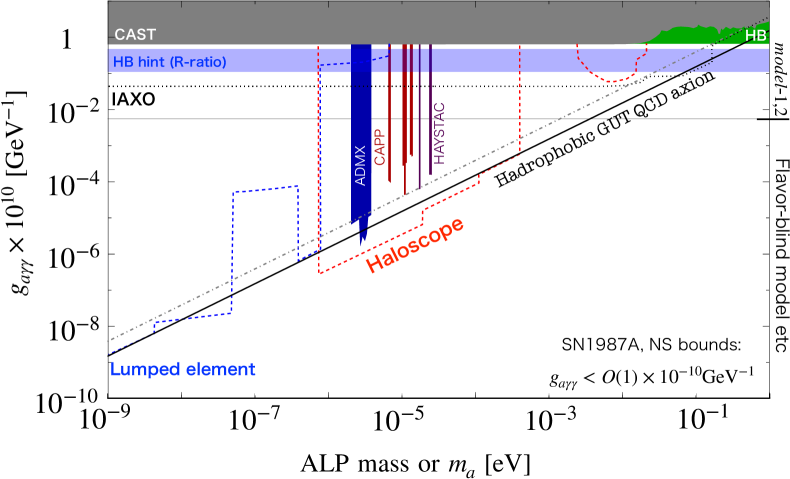
Figure 1: The parameter region of the hadrophobic GUT axion (black solid line) in the $m_{a}-g_{a\gamma\gamma}$ plane. The KSVZ axion is denoted by the gray dot-dashed line, the black solid line below which is the hadrophobic GUT axion (the usual DFSZ axion). The bounds from solar axion observation by CAST (gray shaded region), HB (green shaded region) are shown. Also shown are the future reaches of the IAXO (black thin dotted line). The cooling hint from HB is in the horizontal blue range. The haloscope bounds from ADMX (blue shaded region), CAPP (red shaded region), and HAYSTAC (purple shaded region) experiments assume that the axion composes the dominant component of DM. The future sensitivity region of the lumped element and haloscope experiments are above the blue and red dashed lines, respectively.

In the figure, we have included the bounds from the solar axion observation by CAST (gray shaded region) [82], the HB cooling (green shaded region) [83, 84, 85, 86, 87, 88, 89], and current DM haloscope searches of ADMX (blue shaded region) [90], CAPP (red shaded region) [91, 92] and HAYSTAC (purple shaded region) [93]. The future reaches of IAXO (black dashed line) [44, 45, 46, 47], lumped element experiments (blue dashed line), and haloscope experiments (red dashed line) are also shown (see e.g. Refs. [94, 95, 96, 97, 98, 99, 100]). The reaches and bounds of the lumped element experiments and haloscopes are adopted from Refs. [101]. We note that the axion DM search experiments assume the axion is the dominant component of DM. Interestingly, our QCD axion model can be tested in most of the parameter regions.

We also plot the hint for the extra cooling based on the $R$-parameter as the horizontal blue region (see Eq. (116) in the appendix), where we neglect the top-induced electron coupling, which is justified in the normal embedding of the model 1. Interestingly, the hint and our prediction overlap in the region that can be probed by the IAXO and TASTE [48]. Moreover, if we consider the inverted embedding of model 1 or model 2, the TRGB hint (see Eq. (26)) can also be explained with $\Lambda_{\rm cutoff}=10-100{\rm\,TeV}$ in this range. The cooling hint for the Cassiopeia A neutron star [25, 102] also overlaps, although this hint may not be supported by the subsequent analysis [27, 29]. The region is slightly in tension with the $K^{+}\to\pi^{+}a$ decay bound, but this can be alleviated by introducing a flavor violating coupling and mild tuning (see Fig. 7 and the explanation in the main text). In any case, this region can change the cooling of different stars. So our axion can be probed by further observations of the NSs and by a better understanding of the cooling mechanism. In addition, a large part of the parameter space can be probed in laser-based collider experiments [49, 50, 51, 52], and the aforementioned $K^{+}\to\pi^{+}a$ in the NA62 [66] and KOTO [67] experiments in the future. For the latter, see Fig. 7.

The QCD axion in this interesting region with $g_{a\gamma\gamma}\sim 10^{-10}{\rm\,GeV}^{-1}$ has a relatively heavy mass for the QCD axion, and one has to increase the axion abundance to explain all DM. Although the original misalignment mechanism [1, 2, 3] suffers from a serious isocurvature problem when the anharmonic effect is strong [103, 104], the axion may be produced from the inflaton decay whose reheating temperature is higher than the inflaton mass [105, 106]. In this case, the Bose-enhancement effect is under control in the narrow resonance region.

We note that in realistic models we may have a non-trivial domain wall number. If we consider post-inflationary PQ-breaking models, we need to break the PQ symmetry slightly to let the string domain wall system collapse. Avoiding the quality problem of PQ symmetry (by assuming some discrete symmetry) without tuning, it has been discussed that there is an overproduction problem of axion DM in the DFSZ model unless the decay constant is comparable to or slightly below the ordinary SN1987A bound (e.g., [107]). In our scenario, however, the decay constant can be smaller than usual, which means that a larger bias can be consistent with the required quality of the PQ quality, and a smaller domain wall stress is also allowed. Thus, we can successfully have the mechanism of DM production from domain wall annihilation.

4 Flavor models for hadrophobic and electrophobic GUT axion

In this section, we present two specific models to show that the non-trivial PQ charge assignment required for $v_{a}\lesssim 10^{9}{\rm\,GeV}$ in the previous section can be realized. We focus on the normal embedding of model 1. We show in both UV models that the first two generation quark masses are naturally suppressed.

The flavor-blind charge assignment, which is useful for $v_{a}\gtrsim 10^{9}{\rm\,GeV}$, is straightforward based on the discussions in this section. We will not discuss it explicitly. However, we would like to emphasize that the PQ breaking effect must be large enough to generate the top Yukawa coupling of $\mathcal{O}(1)$, because for the flavor-blind charge assignment, the top Yukawa coupling is forbidden in the PQ symmetric phase. In this case, the ordinary GUT embedding of the quarks and leptons can be fine.

4.1 A three Higgs doublet model

A UV realization can be obtained from three Higgs doublet models. Let us consider a Lagrangian with three Higgs doublets, $H_{0,1,2}$ and a PQ scalar field, $\Phi_{\rm PQ}$, and their PQ charges are given by

Fields	$\Phi_{\rm PQ}$	$5_{H_{0}}$	$5_{H_{1}}$	$5_{H_{2}}$	$10_{1,2}$	$10_{3}$	$\bar{5}_{1,2,3}$
PQ charge$\times 3/c_{5}$	1	0	1	-2	1	0	0

Here, $10_{x}$ and $\bar{5}_{x}$ have the PQ charge assignments of the normal embedding in model 1. The three Higgs fields are introduced to have Yukawa couplings for all the fermions. Note that the charge assignment is determined by the hadrophobic and electrophobic conditions in the previous section, and this does not guarantee that the above charge assignment correctly reproduces the anomaly coefficient $c_{5}$. As we will see later, the anomaly coefficient would be different if we assume the above matter content, and we need to add additional matter fields to correctly reproduce the anomalous couplings to the SM gauge bosons.

A part of the Higgs potential including the PQ scalar is given by

$${V}\supset\left(A\Phi_{\rm PQ}5_{H_{0}}5^{*}_{H_{1}}+\lambda(\Phi_{\rm PQ})^{2}5_{H_{2}}5^{*}_{H_{0}}+h.c.\right)-m_{\Phi}^{2}|\Phi_{\rm PQ}|^{2}+\frac{\lambda_{\Phi}}{2}|\Phi_{\rm PQ}|^{4},$$ (46)

where $A,\lambda,\lambda_{\Phi}$ are coupling constants, and $m_{\Phi}^{2}$ is the mass squared of $\Phi_{\rm PQ}.$ In addition, we can also have some portal couplings, e.g. $|H_{2}|^{2}|\Phi_{\rm PQ}|^{2}$. Here we assume they are small enough to simplify the following discussion. In addition to the above potential, we assume that the Higgs fields have the ordinary potential allowed by the symmetry.

The Yukawa couplings are given by

$$-{\cal L}_{\rm Yukawa} =\sum_{x,y\neq 3}Y_{10;xy}5_{H_{2}}10_{x}10_{y}+Y_{5;xy}5_{H_{1}}^{*}\bar{5}_{x}10_{y}$$ (47)

$$+\sum_{x\neq 3}Y_{5;3x}5_{H_{1}}^{*}\bar{5}_{3}10_{x}+Y_{5;x3}5^{*}_{H_{0}}\bar{5}_{x}10_{3}$$ (48)

$$+(Y_{10;33}5_{H_{0}}10_{3}10_{3}+Y_{5;33}5^{*}_{H_{0}}\bar{5}_{3}10_{3})+h.c.$$ (49)

Let us assume that $m^{2}_{\Phi}(>0)$ is much larger than the EW scale. Then, the PQ symmetry breaking is triggered when $\Phi_{\rm PQ}$ develops a nonzero VEV. We assume that the the colored Higgs has a mass around the GUT scale $\sim 10^{15}{\rm\,GeV}$. Below the GUT scale, we have the PQ breaking at the scale of $m_{\Phi},$ and $\left\langle{\Phi_{\rm PQ}}\right\rangle=v_{a}\approx\sqrt{m_{\Phi}^{2}/\lambda_{\Phi}}.$ Then we get the mixing term between $H_{0}$ and $H_{1,2}$. Suppose that $H_{\rm 1,2}$ have a positive mass squared $m_{H}^{2}$, which satisfies $m_{H}^{2}\gg v_{\rm EW}^{2},Av_{\rm EW}$ and $m_{H}^{2}\lesssim\mathcal{O}(m^{2}_{\Phi})$, where $v_{\rm EW}\sim 170{\rm\,GeV}$ is the VEV of the SM-like Higgs. The inequality implies that the SM-like Higgs boson mass is obtained by fine-tuning, on which we will comment later. Then we can safely integrate out the radial mode of the PQ Higgs boson, $s$, which is defined by the expansion, $\Phi_{\rm PQ}=(v_{a}+s/\sqrt{2})\exp{(ia/\sqrt{2}v_{a})}$.

Let us obtain the mass eigenstates in the effective potential of $H_{1},H_{2},H_{0},\leavevmode\nobreak\ {\rm and}\leavevmode\nobreak\ a$. To simplify the discussion we take $Av_{a}\ll m_{H}^{2}$ and $\lambda v_{a}^{2}\ll m_{H}^{2}$. Then, the mixing between the Higgs fields are suppressed as follows,

$$\theta_{H_{0}H_{1}}\sim\frac{Av_{a}}{m^{2}_{H}}\ll 1,\leavevmode\nobreak\ {\rm and}\leavevmode\nobreak\ \leavevmode\nobreak\ \theta_{H_{0}H_{2}}\sim\frac{\lambda v_{a}^{2}}{m^{2}_{H}}\ll 1.$$ (50)

Since $H_{2},H_{1}$ are heavy, the SM-like Higgs is mostly composed of $H_{0}.$ In this limit, we can neglect the correction to the PQ charge via the mixing of the Higgs fields. The resulting EFT contains the SM fermions with the same quantized PQ charge assignment as in the UV model. In the unitary gauge, $\left\langle{H_{0}}\right\rangle\simeq v_{\rm EW}$ is real. Then we cannot use the rotation of the SM Higgs field to remove $a$ in the effective potential,

$$V_{\rm eff}\approx\lambda v_{a}^{2}e^{i\sqrt{2}a/v_{a}}H_{2}H^{*}_{0}+Av_{a}e^{ia/\sqrt{2}v_{a}}H^{*}_{1}H_{0}+h.c..$$ (51)

On the other hand, we can remove $a$ by redefining $H_{1},H_{2}$. Then, $a$ appears in the Yukawa terms, e.g.

$$y_{u,11}H_{2}Q_{1}u_{1}\to y_{u,11}H_{2}e^{-i\sqrt{2}a/v_{a}}Q_{1}u_{1},y_{d,11}H^{*}_{1}Q_{1}d_{1}\to y_{d,11}H^{*}_{1}e^{-ia/\sqrt{2}v_{a}}Q_{1}d_{1}$$ (52)

and the kinetic terms of $H_{1,2}$. In addition, we can remove $a$ from the Yukawa terms via the chiral rotation of $10_{1,2}$ completely. Then we arrive at the form of Eq. (14) with the desired charge assignment. From the tad-pole conditions, we obtain,

$$\left\langle{H_{1}}\right\rangle\simeq\theta_{H_{0}H_{1}}v_{\rm EW},\leavevmode\nobreak\ \leavevmode\nobreak\ \left\langle{H_{2}}\right\rangle\simeq\theta_{H_{0}H_{2}}v_{\rm EW}.$$ (53)

The quark flavor structure can be obtained following the MFV assumption. For instance, we can take the diagonal up-type quark Yukawa matrix, ${Y}_{10;IJ}\theta_{H_{0}H_{2}}=\delta_{IJ}{y}_{uJ}$ for $I,J=u,c$, and otherwise ${Y}_{10;IJ}=\delta_{IJ}\,{{y}_{uJ}}$. Then, ${Y}_{5;IJ}\theta_{H_{0}H_{1}}=y_{dI}(V_{\rm CKM}^{-1})_{IJ}$ for ${I,J}=u,c$, and otherwise ${Y}_{5;IJ}=y_{dI}(V^{-1}_{\rm CKM})_{IJ}$. Here, we replaced the indices in the l.h.s to be the flavor one, which is allowed due to the assumption of the alignment; $y_{u;IJ}=\delta_{IJ}y_{uJ}$ and $y_{d;IJ}=y_{dI}(V^{-1}_{\rm CKM})_{IJ}$ are the SM Yukawa matrices in the SM Lagrangian,

$${\cal L}\supset-\sum_{I,J=1}^{3}\left(y_{u;IJ}\tilde{H}^{*}Q_{I}\bar{u}_{J}+y_{d;IJ}H^{*}\bar{d}_{I}Q_{J}\right)+{h.c.},$$ (54)

where $H$ and $\tilde{H}$ are the SM-Higgs doublet and its conjugate, respectively, and we explicitly show the bars on $\bar{u}_{J}$ and $\bar{d}_{I}$ as in the conventional notation for the Yukawa interaction. This model can explain the smallness of the up, down, charm, strange, $\mu,\tau$ masses compared to the top quark mass if $|\theta_{H_{0}H_{1}}|,|\theta_{H_{0}H_{2}}|<1$. However, the quark-lepton mass relation, especially the small electron mass compared to the bottom mass, cannot be explained naturally. Note that, as we have seen in the previous section, the right-handed electron must be in $10_{3}$. One solution to these problems is to use the GUT-breaking correction. One can introduce higher dimensional operators such as

$$\delta{\cal L}\supset\frac{\left\langle{\Phi_{\rm GUT}}\right\rangle}{M_{*}}H\bar{L}_{e}e_{R}+h.c.,$$ (55)

where $\Phi_{\rm GUT}$ is the GUT Higgs field responsible for the GUT breaking, $M_{*}$ is the cutoff scale, and $e_{R}$ denotes the right-handed electron. This term could cancel the electron Yukawa coupling and reduce it to the observed value, changing the bottom-electron mass relation predicted by the GUT. This cancellation might be understood in terms of the anthropic selection [80]. For $x=1,2$, the renormalization group running between $v_{a}$ and the GUT scale may change the mass relations for $\{\tau,s\}$, and $\{\mu,d\}$ to obtain the factor $\mathcal{O}(10)$ hierarchy if the corresponding $Y_{5}$ is of order unity in the PQ symmetry phase.

In the low-energy EFT obtained by integrating out $\Phi_{\rm PQ}$ and ${H_{1,2}}$, we have the desired PQ charge assignment of the fermions. However, the chiral anomaly is different from the hadrophobic conditions discussed in the previous section. Indeed, for the above matter content and charge assignment, the anomaly coefficient would be

$$\frac{c_{5}}{3}\left(2\times 3\right)=2c_{5}\neq c_{5}$$ (56)

(or we may also focus on the color subgroup ($\frac{c_{3}}{3}(2\times 2+1\times 2)=2c_{3}$). To match the anomaly coefficient we need additional fields that carry the PQ charge, such as

$${\cal L}\supset\Phi_{\rm PQ}\bar{10}_{\rm PQ}10_{\rm PQ}+{\rm h.c.}$$ (57)

with ${10_{\rm PQ},\bar{10}_{\rm PQ}}$ being a pair of extra PQ fermions which have the total PQ charge $-c_{5}/3$. With the $\Phi_{\rm PQ}$ VEV, $10_{\rm PQ}\leavevmode\nobreak\ {\rm and}\leavevmode\nobreak\ \bar{10}_{\rm PQ}$ become massive. Integrating them out induces an anomalous coupling to the gauge bosons, similar to the KSVZ axion. Since this is a complete GUT multiplet, the resulting axion gauge couplings are universal.

4.2 A vector-like fermion model

We provide an alternative UV realization that does not involve the doublet-triplet splitting problem of the additional Higgs fields. We introduce PQ fermions instead of additional bosonic fields to describe the Yukawa interactions. The PQ charge assignment is

Fields	$\Phi_{\rm PQ}$	$\bar{5}_{{\rm PQ};1,2}$	$5_{{\rm PQ};1,2}$	$\bar{10}_{{\rm PQ};1,2}$	$10_{{\rm PQ};1,2}$	$10_{1,2}$	$10_{3}$	$\bar{5}_{1,2,3}$	$5_{H}$
PQ charge$\times 3/c_{5}$	1	-1	0	0	-1	1	0	0	0

where the extra PQ fermions as well as the PQ Higgs are indicated with the subscript “PQ”.

We consider the renormalizable potential for the PQ Higgs given by

$${V}=-m_{\Phi}^{2}|\Phi_{\rm PQ}|^{2}+\frac{\lambda_{\Phi}}{2}|\Phi_{\rm PQ}|^{4},$$ (58)

which leads to $\left\langle{\Phi_{\rm PQ}}\right\rangle=v_{a}.$ In the EFT after integrating out the PQ Higgs we can replace $\Phi_{\rm PQ}=v_{a}\exp(ia/\sqrt{2}v_{a}).$ The fermion interactions allowed by the symmetry include the following Yukawa couplings,

$${\cal L}_{\rm Yukawa}= \sum_{xy=1,2}Y_{5,xy}\Phi_{\rm PQ}\bar{5}_{{\rm PQ},x}5_{{\rm PQ},y}+M_{5,xy}\bar{5}_{x}5_{{\rm PQ},y}+Y_{d,xy}5^{*}_{H}\bar{5}_{{\rm PQ},x}10_{y}$$ (59)

$$+ \sum_{xy=1,2}Y_{10,xy}\Phi_{\rm PQ}\bar{10}_{{\rm PQ},x}10_{{\rm PQ},y}+Y_{{\rm 10mix},xy}\Phi^{*}_{\rm PQ}\bar{10}_{{\rm PQ},x}10_{y}+Y_{u,xy}5_{H}10_{x}10_{{\rm PQ},y}$$ (60)

$$+ \sum_{x=1,2}M_{10,x3}\bar{10}_{{\rm PQ},x}10_{3}+M_{5,3x}\bar{5}_{3}5_{{\rm PQ},x}+Y_{d,x3}5^{*}_{H}\bar{5}_{x}10_{3}$$ (61)

$$+ Y_{d33}5^{*}_{H}\bar{5}_{3}10_{3}+Y_{u33}5_{H}10_{3}10_{3}.$$ (62)

We have not included interactions such as $5_{H}5_{\rm PQ}\bar{10}_{\rm PQ},5^{*}_{H}\bar{10}_{\rm PQ}\bar{10}_{\rm PQ}$, which are allowed by symmetry but are not important for our discussion. The couplings of these irrelevant interactions are assumed to be small enough to simplify the discussion. We can redefine the fields so that all the phases of $\exp{(ia/\sqrt{2}v_{a})}$ are removed and the axion has only derivative couplings. Then we have the desired form for $10_{x}$ and $\bar{5}_{y}$ for the model 1. Assuming $y_{5}\left\langle{\Phi_{\rm PQ}}\right\rangle\gg M_{5},y_{10}\left\langle{\Phi_{\rm PQ}}\right\rangle\gg M_{10},y_{10\rm mix}\left\langle{\Phi_{\rm PQ}}\right\rangle$, we get a mixing between $\bar{5}_{x}$ and $\bar{5}_{{\rm PQ},y}$, and between $10_{x}$ and $10_{{\rm PQ},y}$, whose mixing parameters are

$$\theta_{5}\sim\frac{M_{5}}{Y_{5}\left\langle{\Phi_{\rm PQ}}\right\rangle}\leavevmode\nobreak\ {\rm and}\leavevmode\nobreak\ \theta_{10}\sim\frac{Y_{10,{\rm mix}}\left\langle{\Phi_{\rm PQ}^{*}}\right\rangle}{Y_{10}\left\langle{\Phi_{\rm PQ}}\right\rangle},\frac{M_{10}}{Y_{10}\left\langle{\Phi_{\rm PQ}}\right\rangle},$$ (63)

respectively. Here we have omitted the flavor index.

We can integrate out BSM particles to obtain the SM Yukawa couplings. This is done by replacing the PQ fermion with mixed SM fermions in the last terms of Eqs. (59) and (60),

$$\delta{\cal L}_{\rm eff}\sim\frac{M_{5}}{Y_{5}\left\langle{\Phi_{\rm PQ}}\right\rangle}5_{H}^{*}10_{1,2}\bar{5}_{1,2,3}+\frac{Y_{10\rm mix}\left\langle{\Phi^{*}_{\rm PQ}}\right\rangle}{Y_{10}\left\langle{\Phi_{\rm PQ}}\right\rangle}5_{H}10_{1,2}{10}_{1,2}+\frac{M_{10}}{Y_{10}\left\langle{\Phi_{\rm PQ}}\right\rangle}5_{H}10_{1,2}{10}_{3},$$ (64)

where we have used short handed notations, and ignored the indices in the Yukawa and mass matrices. The first term involves the 3 generations of $\bar{5}$ because, $5_{{\rm PQ},1,2}$ can mix with all of $\bar{5}$ (see the 2nd terms of Eqs. (59) and (61)). Again we can have a generic 3 by 3 Yukawa matrix for the down-type quark $y_{d;IJ}$ and thus the flavor structure can be obtained. Also the induced Yukawa component by the fermionic mixings are naturally suppressed.

For the desired gauge anomalous coefficient for the hadrophobic axion as discussed in the previous section, we need additional vector-like fermions, $\bar{5^{\prime}}_{\rm PQ},5^{\prime}_{\rm PQ}$, with the coupling of

$$\Phi_{\rm PQ}\bar{5^{\prime}}_{\rm PQ}5^{\prime}_{\rm PQ}.$$ (65)

We have checked that the gluon coupling is still asymptotically free with these additional quarks and thus the gauge coupling unification remains perturbative.

Before concluding this section, we would like to point out that both models considered above have fine-tuning and hierarchy problems between the EW scale, the PQ scale, and the GUT scale. These issues may suggest a suitable UV completion for the models, such as a SUSY extension. Although we do not present a specific UV completion in this paper, we note that it may be straightforward if the additional scalars/fermions in the two models possess a mass scale relevant to the cutoff scale of the effective theory, for example, the soft SUSY breaking scale. In this scenario, the axion decay constant is approximately the cutoff scale (see a related model in [77]). Interestingly, the resolution of the hierarchy problem between the cutoff scale and the EW scale favors a small axion decay constant, making our discussion of the hadrophobic axion significant.

More generally, if the decay constant of the light axion originating from the ${\rm SU{(}}5)\times\mathop{\rm U}(1)_{\rm PQ}$ is related to the cutoff scale to which the EW mass is sensitive, and if the axion couples to the gauge fields, the solution of the hierarchy problem would favor hadrophobic and electrophobic axions.

5 Axionic unification of inflaton and DM consistent in GUT context

The idea of unifying the inflaton and DM goes back to the seminal papers [108, 109], and has been studied in recent works as well [110, 111, 112, 42, 43, 113, 114, 115, 116, 117, 118]. Here we consider the ALP miracle, a unified explanation of inflaton and DM using axion [42, 43].

In the ALP miracle scenario, ALP was assumed to interact primarily with photons (and the SM fermions) at low energies and not to couple to gluons. This is because the astrophysical bounds based on the SN 1987A and NSs severely restrict the coupling of ALP to gluons. For this reason, it was considered that the ALP cannot have a universal coupling to SM gauge bosons, and therefore this scenario is difficult to embed in the GUT. Now we know that, as discussed in the previous sections, hadrophobic axion is possible in the GUT framework. Based on this result, we will reconsider the ALP miracle scenario in terms of hadrophobic axion. In this section, we use $\phi$ instead of $a$ to denote the ALP to facilitate comparison with previous literature.

5.1 The original ALP miracle scenario

First, let us briefly review the basic idea of the ALP miracle scenario. See Refs. [42, 43] for details. In the original model, the ALP is assumed to have a potential of the form,

$$V_{\rm inf}(\phi)=\Lambda^{4}\left(\cos\left(\frac{\phi}{f_{\phi}}+\Theta\right)-\frac{\kappa}{n^{2}}\cos\left(n\frac{\phi}{f_{\phi}}\right)\right)+{\rm const.}$$ (66)

where $n$ ($>1$) is an integer and $\kappa$ and $\Theta$ represent the relative amplitude and phase of the two terms, respectively. We assume that the potential in (66) arises from some UV physics other than QCD, and the parameters in the potential are constant in time. For successful inflation, $\Theta$ must be much smaller than unity, and $\kappa$ must be close to unity. Then the potential is very flat near the origin, and slow-roll inflation takes place. In the next subsection, we will introduce the ALP coupling to gluons, which induces another potential term.

The coefficient of $\phi/f_{\phi}$ in the first cosine term defines $f_{\phi}$. The dynamical scale $\Lambda$ sets the inflation scale, and it is fixed at ${\cal O}(10)$ TeV as explained below. The constant term is added to ensure the vanishingly small cosmological constant in the present vacuum. We introduce two cosine terms in the potential because natural inflation [122, 123], which has a single cosine term, is now excluded due to the null observation of the primordial tensor mode [124] (see also [125]). The next simplest possibility of axion inflation is multi-natural inflation [126, 127, 128, 129], which can be realized in certain UV models with extra dimensions [119, 120, 121]. Our potential takes the minimal form of the multi-natural inflation.

In this paper, we mainly focus on the case where $n$ is odd, which implies an upside-down symmetry of the potential under the shift of $\phi\to\phi+\pi f_{\phi}$:

$$V_{\rm inf}(\phi)=-V_{\rm inf}(\phi+\pi f_{\phi})+{\rm const.}$$ (67)

As a consequence of this symmetry, the inflaton mass squared at the potential minimum is equal to the curvature at the potential maximum, but with the opposite sign. We do not consider here the case of even $n$, and refer the reader to Refs. [77, 57] for discussions of this case.

This upside-down symmetric potential makes the inflaton so light at the potential minimum that its mass is comparable to that of the Hubble parameter in inflation. Inflation occurs in the flat region near the potential maximum, $\phi\simeq 0$. The inflation dynamics is similar to the hilltop quartic inflation. When the inflation ends and the axion oscillates about the potential minimum, $\phi/f_{\phi}\simeq\pi$, its couplings to photons and to fermions cause reheating. For the reason explained above, a coupling with gluons is not included in the original set-up.

The first stage of the reheating occurs due to perturbative decay of the inflaton into light particles such as photons, which quickly thermalize to form a hot plasma. These particles in the interacting plasma give screening or thermal masses to the light particles. In the second stage, the perturbative decay is kinematically forbidden due to the backreaction when the thermal mass becomes comparable to the inflaton. Afterwards, the reheating undergoes with scattering and the inflaton condensate efficiently evaporates if the evaporation rate is higher than the Hubble parameter. A characteristic feature of this set-up is that the smaller the oscillation amplitude of the inflaton, the lighter the effective mass of the inflaton, and thus the smaller the reaction rate of this reheating process. For a certain inflationary scale, the rate for the reheating via scattering and the Hubble parameter become comparable at the beginning of reheating. Then, while most of the energy of the inflaton is used to thermalize the SM particles by reheating (specifically, the evaporation process), some of the inflaton condensates remain intact. This remnant of the inflaton condensate becomes DM when the inflaton becomes non-relativistic. The requirement to account for both inflation and DM at the same time determines the inflationary scale of ${\cal O}(10)$ TeV, and the corresponding Hubble parameter of about ${\cal O}(1)$ eV. It is interesting to note that this corresponds to the axion mass of ${\cal O}(0.01-1)$ eV and an axion-photon coupling $g_{a\gamma\gamma}$ of $10^{-12}-10^{-10}$  GeV^-1, which satisfy the current limits and can be explored by future experiments [43, 42]. In such a minimal setup, where inflation occurs with a single axion, it is highly non-trivial that there exists a region that explains inflation and DM simultaneously, and satisfies all the constraints of current observations, and can be explored by future observations. For this reason, this scenario is called the ALP miracle.

5.2 ALP potential by QCD

The main difference between our model and the original ALP inflation described in the previous subsection is that the ALP has a universal anomalous coefficient with respect to the SM gauge group. In particular, the ALP is coupled to gluons. Thus, there is also the QCD contribution to the potential as given by Eq. (13). We restate the potential due to the non-perturbative effect of QCD once again to match the current notation:

$$V_{\rm QCD}(\phi) =-B_{0}f_{\pi}^{2}\sqrt{m_{u}^{2}+m_{d}^{2}+2m_{d}m_{u}\cos{\left[c_{3}\frac{\phi}{f_{\phi}}\right]}},$$ (68)

where we assume

$$f_{\phi}=\sqrt{2}v_{a}$$ (69)

to simplify our argument. The total potential is given by

$$V=V_{\rm inf}(\phi)+V_{\rm QCD}(\phi+(\theta_{\rm QCD}-\pi)f_{\phi}),$$ (70)

where we include a relative phase of the two terms, $\theta_{\rm QCD}-\pi f_{\phi}$, which is generically present. With this definition, $\phi=\pi f_{\phi}$ is the minimum of $V_{\rm QCD}$ when $\theta_{\rm QCD}=0$. The strong CP phase is given by

$$\bar{\theta}_{\rm CP}\equiv\left\langle{\phi}\right\rangle/f_{\phi}-\pi+\theta_{\rm QCD},$$ (71)

where $\left\langle{\phi}\right\rangle$ is the VEV of $\phi$ in the present vacuum. When $\left\langle{\phi}\right\rangle\approx\pi f_{\phi}$, $\theta_{\rm QCD}$ can be interpreted as the strong CP phase. We will neglect the finite temperature effect during inflation, since we focus on the case in which the Gibbons-Hawking temperature, $T_{\rm GH}=H_{\rm inf}/2\pi$, is much lower than the QCD scale, $T_{\rm GH}\ll\chi^{1/4}$.

As we have seen in the previous section, in the absence of $V_{\rm QCD}$, the inflation takes place near the origin, $\phi\approx 0$, and it is stabilized at $\phi/f_{\phi}\approx\pi$ after inflation. The question is whether the inflaton dynamics in the original setup is modified by $V_{\rm QCD}$. We will see that $V_{\rm QCD}$ does not significantly change the inflaton dynamics. This is essential because its potential height is much smaller than the inflaton potential, $V_{\rm QCD}\ll V_{\rm inf}$. However, as we will see, the curvature of $V_{\rm QCD}$ could change the location of the potential minimum and maximum, and thus the strong CP phase.

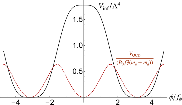
Figure 2: $V_{\rm inf}/\Lambda^{4}$ and $V_{\rm QCD}/(B_{0}f_{\pi}^{2}(m_{u}+m_{d}))$ are shown as a function of $\phi/f_{\phi}$ in black solid and red dashed lines, respectively, where we set $n=3$ and $c_{3}=2$. For illustrative purposes we set $\Theta=0$ and $\theta_{\rm QCD}=0$. A constant term is added to adjust the potential at the minima equal to zero.

In the presence of $V_{\rm QCD}$, the upside-down symmetry no longer holds, regardless of the parity of $c_{3}$ (see Eq. (68)). In Fig. 3 we plot $V^{\prime}_{\rm QCD}(\phi)+V^{\prime}_{\rm QCD}(\phi+\pi f_{\phi})$ (left panel) and $V^{\prime\prime}_{\rm QCD}(\phi)+V^{\prime\prime}_{\rm QCD}(\phi+\pi f_{\phi})$ (right panel) in black solid and red dashed lines, for $c_{3}=1$ and $c_{3}=2$, respectively. The deviation from zero of these functions implies that the upside-down symmetry is explicitly broken by $V_{\rm QCD}$. As a consequence, the first derivative of the potential flips the sign under the shift of $\phi\to\phi+\pi f_{\phi}$ only at $\phi/f_{\phi}=0\leavevmode\nobreak\ {\rm mod}\leavevmode\nobreak\ \pi/2$. This property will be important for a consistent DM cosmology.

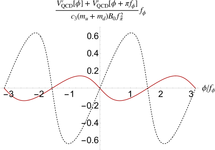
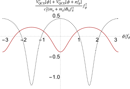
Figure 3: The breaking of the upside-down symmetry induced by the QCD instanton is shown in the red solid and black dashed lines for $c_{3}=1$ (odd) and $2$ (even), respectively. In the left and right, we plot $(V^{\prime}_{\rm QCD}(\phi)+V^{\prime}_{\rm QCD}(\phi+\pi f_{\phi}))f_{\phi}/(c_{3}\chi)$ and $(V^{\prime\prime}_{\rm QCD}(\phi)+V^{\prime\prime}_{\rm QCD}(\phi+\pi f_{\phi}))/(c_{3}^{2}\chi)$, respectively.

5.3 Viable parameter region for successful inflation

For successful inflation, we assume that the inflaton initially stays in the vicinity of the potential maximum near the origin. Around the origin, the potential can be expanded as

$$V(\phi)=V_{0}-\theta\frac{\Lambda^{4}}{f_{\phi}}{\phi}+\frac{m^{2}}{2}\phi^{2}+A\phi^{3}-\lambda\phi^{4}+\cdots$$ (72)

with

$$V_{0} \simeq\left(2-\frac{2}{n^{2}}\sin^{2}{\frac{n\pi}{2}}\right)\Lambda^{4}$$ (73)

$$\theta \simeq\Theta-(\theta_{\rm QCD}-\pi)\frac{\chi}{\Lambda^{4}}c_{3}$$ (74)

$$m^{2} \simeq\frac{(\kappa-1)}{2}\frac{\Lambda^{4}}{f_{\phi}^{2}}-\frac{1}{2}\frac{\chi}{f_{\phi}^{2}}c_{3}^{2}$$ (75)

$$A \simeq\frac{\Theta}{3!}\frac{\Lambda^{4}}{f_{\phi}^{3}}-\frac{\theta_{\rm QCD}-\pi}{3!}\frac{\chi}{f_{\phi}^{3}}c_{3}^{3}$$ (76)

$$\lambda \simeq\frac{n^{2}-1}{4!}\left(\frac{\Lambda}{f_{\phi}}\right)^{4},$$ (77)

where we have neglected subleading terms. Note that $m^{2}<0$ in the parameters of our interest. For the hilltop inflation, the cubic term has a negligible effect on the inflaton dynamics, and we have [77]

$$|\theta|\lesssim\left(\frac{f_{\phi}}{M_{\rm pl}}\right)^{3},\leavevmode\nobreak\ \leavevmode\nobreak\ |m^{2}|\lesssim\frac{\Lambda^{4}}{f_{\phi}^{2}}\left(\frac{f_{\phi}}{M_{\rm pl}}\right)^{2}.$$ (78)

for $n=O(1)$. On the other hand, we need

$$\theta=\mathcal{O}\left(0.001-0.1\right)\left(\frac{f_{\phi}}{M_{\rm pl}}\right)^{3}$$ (79)

to explain the observed scalar spectral index of the density perturbation [130]. Since the quadratic term is small from the slow-roll condition, by comparing the linear and quartic terms, the location of the potential maximum can be determined as

$$\phi_{\rm max}=\mathcal{O}\left(\frac{f^{2}_{\phi}}{M_{\rm pl}}\right).$$ (80)

This condition does not change much by varying $m^{2}$ within the slow-roll regime.

The difference in the inflation potential from the original ALP inflation potential comes from the cubic term while the additional contributions to the linear and quadratic terms can be absorbed by $\Theta$ and $\kappa$ as can be seen from Eq. (72). To assess the contribution of the cubic term to the inflaton dynamics, we recall that one of the slow-roll conditions at the hilltop, i.e. the condition for hilltop inflation, is given by

$$H_{\rm inf}^{2}\simeq\frac{\Lambda^{4}}{3M^{2}_{\rm pl}}\gtrsim|V^{\prime\prime}(\phi_{\rm max})|$$ (81)

Indeed, the conditions of Eq. (78) can be obtained by requiring each contribution from the quadratic and quartic terms at the hilltop to satisfy the inequality. We can also restrict the cubic coupilng $A$ using this condition. It turns out that

$$\frac{|A|}{\Lambda^{4}/f^{2}_{\phi}M_{\rm pl}}<\mathcal{O}(1).$$ (82)

The QCD potential contributes to the cubic term as

$$\frac{\delta A}{\Lambda^{4}/f_{\phi}^{2}M_{\rm pl}}=-10^{-11}(\theta_{\rm QCD}-\pi)c_{3}^{3}\left(\frac{\Lambda}{10^{4}{\rm\,GeV}}\right)^{-4}\left(\frac{f_{\phi}}{10^{8}{\rm\,GeV}}\right)^{-1}.$$ (83)

Since $|\theta_{\rm QCD}-\pi|\lesssim{\cal O}(1)$, this contribution is always negligible in inflationary dynamics.

In summary, the inclusion of $V_{\rm QCD}$ does not change the inflationary dynamics from the original ALP miracle scenario. Therefore, we can safely use the results of the previous studies [126, 127, 128, 129, 42, 43, 77], and in particular, the CMB normalization fixes the quartic coupling as

$$\lambda\simeq 10^{-12}\leavevmode\nobreak\ \leavevmode\nobreak\ \leavevmode\nobreak\ \text{[CMB normalization]}$$ (84)

in the parameter range of interest. This is a general property of the hilltop quartic inflation. Similarly, the observed spectral index can be explained if

$$|V^{\prime\prime}(\phi_{\rm max})|=\zeta H_{\rm inf}^{2}\leavevmode\nobreak\ \leavevmode\nobreak\ \leavevmode\nobreak\ \leavevmode\nobreak\ \text{[spectral index]}$$ (85)

with $\zeta=\mathcal{O}(0.01-1)$. We also note that in the low scale inflation like the one considered here, the tensor-to-scalar ratio is predicted to be extremely small, $r\simeq 2\times 10^{-47}\left(\frac{H_{\rm inf}}{1{\rm\,eV}}\right)^{2}$, which is of course consistent with the current limit, $r<0.036(95\%{\rm CL})$  [124].

5.4 ALP mass and the strong CP problem

Now let us discuss the ALP around the potential minimum. In this case, the QCD instanton contribution becomes important since it breaks the upside-down symmetry.

The potential around $\phi=\pi f_{\phi}$ is given by

$$V(\phi)\simeq\tilde{\theta}\frac{\Lambda^{4}}{f_{\phi}}{(\phi-\pi f_{\phi})}-\frac{\tilde{m}^{2}}{2}(\phi-\pi f_{\phi})^{2}-\tilde{A}(\phi-\pi f_{\phi})^{3}+\lambda(\phi-\pi f_{\phi})^{4}.$$ (86)

If the QCD contribution were neglected, we would obtain $\tilde{\theta}=\theta$, $\tilde{m}^{2}=m^{2}$, and $\tilde{A}=A$ because of the upside-down symmetry. Note that $\tilde{m}^{2}<0$ in this definition. Then the ALP mass at the potential minimum, $m_{\phi}$ would be given by

$$m_{\phi}^{2}=\zeta H^{2}_{\rm inf}\leavevmode\nobreak\ \leavevmode\nobreak\ \leavevmode\nobreak\ \leavevmode\nobreak\ \leavevmode\nobreak\ [\text{upside-down symmetric limit}],$$ (87)

which is fixed by the spectral index (see Eq. (85)). Because of this property, the ALP remains light in the present vacuum, and it can be stable enough to become DM.

However, as we have seen above, the upside-down symmetry is explicitly broken by the QCD contribution. The linear term happens to be equal in magnitude and opposite in sign at $\theta_{\rm QCD}=0\leavevmode\nobreak\ \leavevmode\nobreak\ ({\rm mod}\leavevmode\nobreak\ \leavevmode\nobreak\ \pi/2)$. See Fig. 3. In the regions around $\theta_{\rm QCD}\approx\pi/2,\pi,3\pi/2$, however, the expansion in the above does not work or/and the strong CP phase will be too large to be consistent with the experimental bound. So we will focus on the case of $|\theta_{\rm QCD}|\ll 1$. In this case, we obtain

$$\tilde{\theta}-\theta\simeq\mathcal{O}(0.1-1)\theta_{\rm QCD}\frac{\chi}{\Lambda^{4}}c_{3},$$ (88)

which is induced by a small relative phase between $V_{\rm inf}$ and $V_{\rm QCD}$.

In the following we give an analytical estimate of the additional contributions to the ALP mass at the potential minimum. First, the change of the linear term (88) induces an extra contribution to the ALP mass, which comes from the balance between the linear term and the quartic term. Denoting this contribution by $\delta_{\rm CPV}m_{\phi}^{2}$, we obtain

$$\delta_{\rm CPV}m_{\phi}^{2}\sim 10^{-11}{\rm\,GeV}^{2}|\theta_{\rm QCD}|^{2/3}\left(\frac{10^{7}{\rm\,GeV}}{f_{\phi}/c_{3}}\right)^{2/3}\left(\frac{\lambda}{10^{-12}}\right)^{1/3}.$$ (89)

This contribution is less than $1{\rm\,keV}$ for $|\theta_{\rm QCD}|\lesssim 1$ when $f_{\phi}/c_{3}\gtrsim 10^{7}{\rm\,GeV}$. Note that this contribution vanishes when $\theta_{\rm QCD}\to 0$.

Second, the QCD contribution $V_{\rm QCD}$ contributes to the mass, which does not vanish even when $\theta_{\rm QCD}=0$. In fact, the quadratic terms at $\phi=0$ and $\phi=\pi f_{\phi}$ are related as

$$\tilde{m}^{2}=m^{2}-V_{\rm QCD}^{\prime\prime}(0)-V_{\rm QCD}^{\prime\prime}(\pi f_{\phi}).$$ (90)

The upside-down symmetry breaking contribution to the quadratic term, $V_{\rm QCD}^{\prime\prime}(0)+V_{\rm QCD}^{\prime\prime}(\pi f_{\phi})=\mathcal{O}(0.1-1)c_{3}^{2}\chi/f_{\phi}^{2}$, is positive (negative) if $c_{3}$ is even (odd) when $\theta_{\rm QCD}\to 0$. See Fig. 3. This is the additional correction to the ALP mass, which arises from the explicit breaking of the upside-down symmetry of $V_{\rm QCD}$. Note that the sign of this contribution depends on the parity of $c_{3}$. When $c_{3}$ is odd, there might be some cancellation. In particular, the ALP mass may be smaller than $c_{3}^{2}\chi/f_{\phi}^{2}$ by a factor of $\xi_{T}$. This is due to the cancellation between $\left(V_{\rm QCD}^{\prime\prime}[0]+V_{\rm QCD}^{\prime\prime}[\pi f_{\phi}]\right)$ and other contributions.

To sum up, the ALP mass is obtained by the largest of the three contributions,

$$m_{\phi}=\sqrt{\max[\zeta H^{2}_{\rm inf},\delta_{\rm CPV}m_{\phi}^{2},\xi_{T}c_{3}^{2}\chi/f^{2}_{\phi}]}.$$ (91)

We set $\xi_{T}=0.1(0.43)$ for the odd (even) values of $c_{3}$. The choice of $\xi_{T}$ in the even case is based on numerical calculations. In the case of odd values, we have taken into account the cancellation of positive and negative contributions, which amounts to about $10\%$.

In Fig.4 we plot the prediction of $\theta_{\rm QCD}$ with respect to $m_{\phi}$ by stabilizing the potential, for $c_{3}=1$ (red circle points) and $c_{3}=2$ (black triangle points) in the left and right panels, respectively. Here we randomly take $\log_{10}{\theta\left(f_{\phi}/M_{\rm pl}\right)^{-3}}=[-3,0]$, $\log_{10}[-V^{\prime\prime}/H_{\rm inf}^{2}]|_{\rm hilltop}=[-3,0]$, and $\log_{\rm 10}|\theta_{\rm QCD}|=[-15,-5]$ with both signs. We fix $\lambda=10^{-12}$ and $n=3$, $f_{\phi}=10^{8}\,$GeV. In the lower mass region the contribution of $H_{\rm inf}^{2}\xi$ in Eq. (91) is dominant, while $\delta_{\rm CPV}m_{\phi}^{2}$ is dominant at larger mass scale. In Fig. 5 we show the cases for $f_{\phi}=10^{7}{\rm\,GeV},10^{6}{\rm\,GeV}$. In this case, the dominant contribution at smaller $|\theta_{\rm QCD}|$ is from $\xi_{T}c_{3}^{2}\chi/f_{\phi}^{2}$ in Eq. (91). This contribution is the same as the ordinary QCD axion. It increases when $f_{\phi}$ decreases. For odd $c_{3}$, there is a mild cancellation between the contributions of $\delta_{\rm CPV}m_{\phi}^{2}$ and $\xi_{T}c_{3}^{2}\chi/f_{\phi}^{2}$. The contribution of $\zeta H_{\rm inf}^{2}$ is negligibly small in the whole range. In Fig. 6, we take $f_{\phi}=2\times 10^{7}{\rm\,GeV}$, in which case there is a region where all three contributions are important. We have confirmed that the analytical estimate of the ALP mass given by Eq. (91) is consistent with the numerical result.

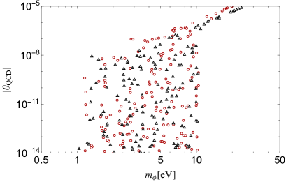
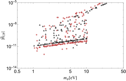
Figure 4: The relative phase, $\theta_{\rm QCD}$ (left panel) and the strong CP phase, $\bar{\theta}_{\rm CP}$ (right panel) with respect to the ALP DM mass, $m_{\phi}$, evaluated at the potential minimum. We consider $f_{\phi}=10^{8}{\rm\,GeV}$ with $c_{3}=1$ (red circles) and $c_{3}=2$ (black triangles). The hot DM mass limit, $m_{\phi}\lesssim 1{\rm\,eV}$, constrains the strong CP phase.

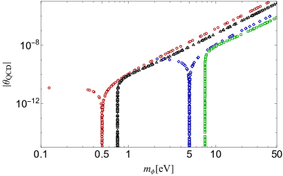
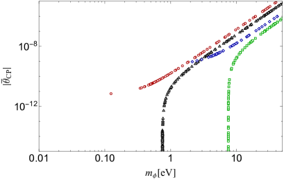
Figure 5: Same as Fig. 4 but with different $f_{\phi}$. Data points of red circles, black triangles, blue diamonds, and green squares represent $(f_{\phi},c_{3})$ values of $(10^{7}{\rm\,GeV},1),(10^{7}{\rm\,GeV},2),(10^{6}{\rm\,GeV},1)$, and $(10^{6}{\rm\,GeV},2)$, respectively. The hot DM mass limit, $m_{\phi}\lesssim 1{\rm\,eV}$, constrains the strong CP phase.

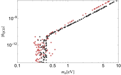
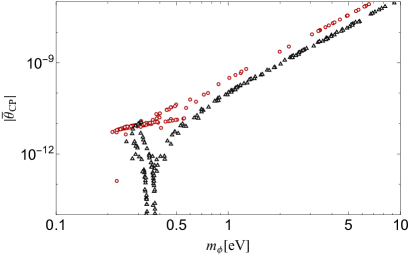
Figure 6: Same as Fig. 4 but with $f_{\phi}=2\times 10^{7}{\rm\,GeV}$. The hot DM mass limit, $m_{\phi}\lesssim 1{\rm\,eV}$, constrains the strong CP phase.

As we will see in the next section, during reheating, ALP particles are produced and thermalized, while the ALP condensate remains as cold DM. The ALP particles decouple after reheating and contribute to the dark radiation with

$$\Delta N_{\rm eff}=\mathcal{O}(0.01).$$ (92)

The abundance fraction of hot DM places an upper bound on the ALP mass of [43] (translated from [133])

$$m_{\phi}<7.7\,{\rm\,eV}\left(\frac{0.03}{\Delta N_{\rm eff}}\right)^{3/4}.$$ (93)

Note that the ALP production from ALP-hadron interaction, including the axion-pion mixing, can be neglected due to the hadrophobia compared to the previously discussed contributions (c.f. [59, 60]). This hot DM mass bound leads to a range for the ALP decay constant,

$$10^{6}{\rm\,GeV}\lesssim f_{\phi}\lesssim 10^{8}{\rm\,GeV}.$$ (94)

The upper bound is from the first term in Eq. (91), while the lower bound is from the last term of Eq. (91). As we will see, this range is also supported by the requirement for successful reheating and the correct DM abundance.

For clarity, the range for $f_{\phi}$ specified in Eq. (94) suggests that the value of $(\langle\phi\rangle/f_{\phi}-\pi)$ is approximately $\mathcal{O}(f_{\phi}/M_{\rm pl})\ll 10^{-10}$. This aligns with the experimental upper limit on the strong CP phase, and is derived from the upside-down symmetry and Eq. (80). The same hot DM bound also constrains $\theta_{\rm QCD}$. By requiring the mass contribution from Eqs. (89) is less than $1{\rm\,eV}$, we derive

$$\boxed{|\theta_{\rm QCD}|,\leavevmode\nobreak\ |\bar{\theta}_{\rm CP}|\lesssim 10^{-9}.}$$ (95)

This result is intriguing as it suggests the suppression of the nucleon EDM. However, it is crucial to note that this does not imply the absence of any fine-tuning for solving the strong CP problem. Instead, it integrates the fine-tuning into the DM sector. The presence of cold DM in the correct abundance, along with the absence of a hot DM component, is crucial for successful structure formation. Thus, the strong CP problem is anthropically resolved (for similar approaches, see Refs. [134, 135, 136, 57, 137]).

We find that the lower limit of the ALP mass, as derived from Eq. (91), is about $0.01{\rm\,eV}\lesssim m_{\phi}$. This results from the first (last) contribution being an increasing (decreasing) function of $f_{\phi}$. We note that, if this bound is satisfied, the structure formation bound for the late-forming DM is also satisfied [42, 43]. Thus, the predicted mass range is

$$0.01{\rm\,eV}\lesssim m_{\phi}\lesssim 1{\rm\,eV},$$ (96)

which is also confirmed by our numerical results.

So far we have assumed the completion of the reheating via the dissipation effect, which leads to the production of thermal ALPs. Thus, the resulting Eqs. (95) and Eq. (94) do not depend on the specific details of the ALP interaction. These conditions help us to identify potential ALP-fermion interactions where the parameter range for successful reheating and DM abundance is consistent with Eq. (94).

5.5 Successful reheating and viable parameter region

Now let us study the reheating process in more detail. To satisfy the bound on $f_{\phi}$ given by Eq. (94), we should focus on the models in Sec. 3.2. It is known that the ALP condensate will completely evaporate and does not explain DM, when $c_{t}=\mathcal{O}(0.1-1)$ in the range of $f_{\phi}$ given by (94) [43, 138]. This leads us to consider the normal embedding of the model 1, which has $c_{t}=0$.

By redefining $10_{1,2}$ to have the ALP in the SM Yukawa coupling phases, we obtain

$${\cal L}_{\rm int}=(2c_{5}-c_{5})\frac{\phi}{f_{\phi}}\sum_{i=1}^{3}\frac{g_{i}^{2}}{32\pi^{2}}F_{i}\tilde{F}_{i}=c_{5}\frac{\phi}{f_{\phi}}\sum_{i=1}^{3}\frac{g_{i}^{2}}{32\pi^{2}}F_{i}\tilde{F}_{i}$$ (97)

Then the interacting Lagrangian in the symmetric phase is

$${\cal L}_{\rm int}\approx-\frac{ic_{5}\phi}{3f_{\phi}}\times\left(2\sum_{x=1,2}y_{ux}HQ_{x}{u}_{Rx}+y_{dx}H^{*}Q_{x}{d}_{R,x}+y_{ex}H^{*}L_{x}{e}_{R,x}\right)+h.c.$$ (98)

where we have dropppted terms of $\mathcal{O}(\phi^{2})$, and $x$ denotes the GUT index related to the mass flavor (see the discussion below Eq. (38)). In the following we neglect the gauge interactions, whose perturbative dissipation rates are known to be less efficient than the dissipation rates from the ALP interactions with tau and charm [43].

After the end of inflation, the ALP field starts to oscillate around its minimum with a large effective mass given by

$$m_{\rm eff}^{2}\sim 12\lambda\phi_{\rm amp}^{2}=\left(35{\rm\,GeV}\right)^{2}\frac{\lambda}{10^{-12}}\left(\frac{\phi_{\rm amp}}{10^{7}{\rm\,GeV}}\right)^{2}.$$ (99)

The first step in the reheating process is the perturbative decay of the ALP condensate, $\phi\to\bar{\psi}_{L}\psi_{R}$, with $\psi$ being a fermion in the Lagrangian (98). The decay rate is given by

$$\Gamma_{{\rm dec},\psi}\simeq\frac{N_{c}}{8\pi}\left(\frac{c_{\psi}m_{\psi}}{f_{\phi}}\right)^{2}m_{\rm eff}.$$ (100)

where $N_{c}$ is the color factor when $\psi$ is a quark (if $\psi$ is a lepton, $N_{c}=1$).

The produced fermions soon thermalize via the SM $2\to 2$ or $2\leftrightarrow 3$ interactions and form a thermal plasma with temperature $T$. This temperature gradually increases as the $\phi$ decay proceeds. Within a Hubble time, $eT\sim m_{\rm eff}$ is satisfied, and then the back reaction becomes important.

The first back-reaction is the thermal blocking effect, which occurs when the phase space for the decay closes due to the sizable thermal mass, e.g. $m_{\rm lepton}^{\rm th}\sim eT.$ Another effect is the dissipation effect due to the scattering of $\phi\psi_{L}\to\psi_{R}\gamma$ and other processes. The dissipation rate is given by [139]

$$\Gamma_{{\rm dis},\psi}\sim 0.5N_{c}\left(\frac{c_{\psi}m_{\psi}}{f_{\phi}}\right)^{2}\left(\frac{\alpha_{\psi}}{2\pi^{2}}\right)T.$$ (101)

Here, $\alpha_{\psi}=\alpha\approx 1/137$ for leptons and $\alpha_{\psi}=\alpha_{s}\approx 0.1$ for quarks. The temperature continues to increase due to this process. When the temperature becomes higher than the weak scale, the scattering $\phi H\to\psi_{L}\psi_{R}$ starts to occur, where $H$ is the Higgs boson. The dissipation rate is given by [144, 43]

$$\Gamma_{\rm dis,\psi}^{\rm sym}\simeq N_{c}\left(\frac{c_{\psi}^{2}y_{\psi}^{2}}{2\pi^{3}f_{\phi}^{2}}\right)T^{3}.$$ (102)

The tau and charm Yukawa interactions give the dominant contribution to these processes.

The most of the initial ALP energy is transferred to thermal plasma, and reheating is successful, if the dissipation rate is larger than the Hubble parameter,

$$\Gamma_{\rm dis,\psi}^{\rm sym}\gtrsim H_{\rm inf}$$ (103)

by using $\frac{107.75\pi^{2}}{30}T^{4}=V_{0}$ to estimate the dissipation rate. The relativistic degrees of freedom $1+106.75=107.75$ will be explained shortly. Let us define the ratio, $\xi\equiv H_{\rm inf}/\Gamma_{\rm dis,\psi}^{\rm sym}$. In the ALP miracle scenario, some of the ALP condensate remains and explains DM. For this scenario, we need $\xi=\mathcal{O}(0.01-0.1)$ [43]. Then we obtain

$$f_{\phi}/c_{5}^{2}=f_{\phi}/c_{3}^{2}\simeq 5.8\times 10^{7}{\rm\,GeV}\frac{\xi}{0.1}\sqrt{\frac{3}{n}}\left(\frac{\lambda}{10^{-12}}\right)^{1/4}.$$ (104)

Since the photon anomaly coefficient, $c_{\gamma}$, satisfies, $c_{\gamma}\equiv c_{5}(1+5/3-1.92)$, the photon coupling is

$$g_{\phi\gamma\gamma}\simeq 1.5\times 10^{-11}{\rm\,GeV}^{-1}c_{3}^{-1}\sqrt{\frac{n}{3}}\left(\frac{\xi}{0.1}\right)^{-1}\left(\frac{\lambda}{10^{-12}}\right)^{-1/4}.$$ (105)

From Eqs. (91) and (104), we obtain a lower bound on the ALP mass $m_{\phi}$, which is relevant to determine the strong CP phase

$$m_{\phi}\gtrsim\sqrt{\delta_{\rm CPV}m^{2}_{\phi}}\sim 0.86{\rm\,eV}c_{3}^{-1/3}\left(\frac{n}{3}\right)^{1/6}\left(\frac{g_{\phi\gamma\gamma}}{1.5\times 10^{-11}{\rm\,GeV}^{-1}}\frac{\theta_{\rm QCD}}{10^{-10}}\right)^{1/3}\left(\frac{\lambda}{10^{-12}}\right)^{1/6}.$$ (106)

In order to achieve successful reheating, i.e. the dominant fraction of the ALP condensate is thermalized, it is predicted that the ALP particle will undergo thermalization and become an additional degree of freedom due to its thermalization rate being almost identical to that given in Eq. (102) [144]. This is why we have a hot DM component, which results in Eqs. (94) and (95). Again, we have checked that requiring the suppression of the hot DM density, $m_{\phi}<7.7{\rm\,eV}$, and Eq. (106) predicts the small strong CP phase.

So far we have focused on the perturbative effect of reheating. In fact, there may also be a non-perturbative effect, namely the sphaleron process , which could introduce friction to the ALP oscillation, potentially decreasing its amplitude, thereby converting the condensate energy into thermal plasma. Clarifying its precise contribution to the reheating is beyond the scope of this work, but we would like to comment on some specific features of our scenario. Due to the negative curvature around the hilltop and large quartic coupling around the potential minimum, a tachyonic resonance and self-resonance occur soon after the inflation, before the end of the reheating process. As a result, a dominant fraction of the inflaton condensate is destroyed within a few oscillations of the ALP field. The resulting ALP condensate has typical energy of $p_{\rm typical}\sim\mathcal{O}(1-10)m_{\rm eff}\sim 10^{-3}\text{-}10^{-1}\Lambda$ [145]. On the other hand, the sphaleron effect is characterized by the magnetic screening scale, $m_{\rm mag}=\mathcal{O}(0.1)g_{i}^{2}T\sim 10^{-2}\Lambda$ (see, e.g., Ref.[146]), where we have used $g_{\star}\pi^{2}/30T^{4}=V_{0}$. Above this scale, the sphaleron rate quickly approaches zero[146]. Therefore, the interaction of excited modes with higher center-of-mass energy than $m_{\rm mag}$ may be irrelevant. In our case, $m_{\rm mag}$ is comparable or slightly smaller than the typical center-of-mass energy between the ALP condensate and the thermal plasma, $\sqrt{Tp_{\rm typical}}=\mathcal{O}(0.01-0.1)\Lambda.$ Therefore, we expect a suppression of the QCD sphaleron rate from the conventional value of $\sim c_{3}^{2}(3\alpha_{3})^{5}T^{3}/f_{\phi}^{2}$. If the suppression is smaller than $\mathcal{O}(0.01)$, our conclusions do not change. The electroweak sphaleron effect is completely neglected in our analysis. However, we stress that a more detailed study of the sphaleron rate will be important.

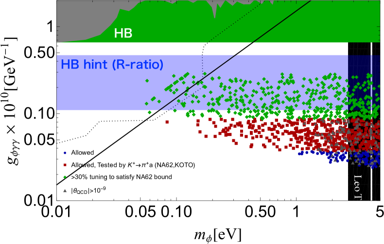
Figure 7: The viable parameter region of the ALP being the inflaton and DM, featuring GUT (red square and blue circle data points), is shown in the $m_{\phi}-g_{\phi\gamma\gamma}$ plane. The black-shaded region indicates the bound from MUSE observations of the Leo T dwarf galaxy [147]. The red squares and green diamonds (with an amount of tuning less than 30% to explain the current bound) will also be tested in future measurements of $K\to\pi a$ in NA62 and KOTO experiments. The bound for the same process is around the HB’s one. The gray triangle points denote the data with $\left|{\theta_{\rm QCD}}\right|>10^{-9}$. Other constraints and hints are the same as in Figure 1.

The scatter plot in Fig.7 shows the parameter region for successful reheating via Eq. (98). We generated data points with varying values of $\log_{10}{\lambda}=[-13,-11]$, $\xi=[0.01,1]$, $\log_{10}{\zeta}=[-2,0]$, $\log_{10}|\theta_{\rm QCD}|=[-19,-5]$, $c_{5}=c_{3}=1,2,\cdots 10$, and $n=3,5,7,9,11$ at random. Using Eqs. (104) and (91), we obtained $f_{\phi}$ and $m_{\phi}$ for each data point and plotted their position in the $m_{\phi}-g_{a\gamma\gamma}$ plane. We also checked the condition (117), but found that it did not affect the viable parameter region. Eqs. (23) affected the parameter region. This bound can be alleviated slightly with a mild tuning by introducing the flavor-violating axion-quark coupling at the beginning to cancel the CKM bound. We show the green diamond points for the amount of tuning less than $30\%$ to have the allowed region, otherwise they are excluded. The red square points will be covered in future observations of $K^{+}\to\pi^{+}a$ via the CKM contribution. The blue circle data points may not be reached via $K^{+}\to\pi^{+}a$ experiments but can be fully tested in the future measurement of $\Delta N_{\rm eff}$ via CMB and BAO experiments, as well as via direct and indirect detections, including intensity mapping[148, 149, 150], and laser-based collider experiments [53] via the ALP photon coupling. The gray diamond points denote the data with $|\theta_{\rm QCD}|>10^{-9}$.

Therefore, we have demonstrated that in order to explain both inflation and DM with an ALP featuring GUT, the parameter region should satisfy $g_{\phi\gamma\gamma}=\mathcal{O}(10^{-11}){\rm\,GeV}^{-1}$, $0.01{\rm\,eV}\lesssim m_{\phi}\lesssim 1{\rm\,eV}$, and $|\theta_{\rm QCD}|<10^{-9}.$ This conclusion is partly due to the fact that the predicted range from cosmology happens to be around the QCD axion parameter region, which depends on the size of the QCD scale, i.e., the Hubble scale and the corresponding QCD-induced mass scale for the decay constant are similar. If the QCD scale were much larger than ours (but much smaller than $\Lambda$), we could not find a parameter region for the ALP to serve as both the inflaton and DM (see Figs.3). If the QCD scale were much smaller than ours, then the strong CP phase would not be suppressed to the same extent. The predicted viable parameter region is consistent with the bounds from stellar cooling, flavor physics, structure formation for the late-forming DM [42, 43], and the neutron EDM. This ALP DM scenario is even hinted at by analyses of stellar cooling and extragalactic background light [151, 152, 153, 154, 155].

6 Conclusions

In this paper, we have investigated the possibility of realizing the hadrophobic axion in the context of GUT. In particular, we have shown that the required PQ charge assignment can be understood on the basis of isospin symmetry. If the hadrophobic axion is the QCD axion, we get the photon coupling as the conventional GUT axion.

Furthermore we have imposed the condition for electrophobia to satisfy the severe astrophysical bound on the axion-electron coupling. Based on both conditions for the hadrophobia and electrophobia we have classified possible PQ charge assignments that are consistent with the SU(5) GUT. The lower end of the axion window for the QCD axion can be slightly relaxed due to the hadrophobic and electrophobic nature. This revives the region where the axion can explain some stellar cooling hints simultaneously. This interesting region can be fully tested in the future. There are also implications for the flavor physics, since it enhances the branching fraction of $K^{+}\to\pi^{+}+\,$missing which can be observed in the KOTO and NA62 experiments. Most of the viable parameter regions where the QCD axion is the dominant component of DM will be tested in the future haloscope and lumped element experiments.

Finally, we have studied a scenario, where an ALP plays both roles of the inflaton and DM, and shown that it is compatible with a viable model of the GUT EFT. Requiring the ALP as the inflaton and DM, the viable parameter region points to

$$g_{\phi\gamma\gamma}=\mathcal{O}(10^{-11}){\rm\,GeV}^{-1},0.01{\rm\,eV}\lesssim m_{\phi}\lesssim 1{\rm\,eV}\leavevmode\nobreak\ {\rm and}\leavevmode\nobreak\ |\bar{\theta}_{\rm CP}\leavevmode\nobreak\ {\rm mod}\leavevmode\nobreak\ \pi|\lesssim 10^{-9}.$$ (107)

Interestingly, in most of the above parameter regions, the strong CP problem is solved, and this scenario can be fully tested not only from the K-meson decay and star coolings, but also from the future measurement of the $\Delta N_{\rm eff}$, direct/indirect detections, (the absence of) the primordial tensor mode, and EDM.

Once the axion DM is found, it could further become a probe of the origin of GUTs and flavors by measuring the axion couplings with fermions and photons.

Note added: While this paper was being submitted, Ref. [156] appeared on arXiv. The authors discussed the (non-GUT) hadrophobic axion with the emphasis on the quantized charge assignment of Eq. (8) as well as the interpretation by using the isospin conservation. In fact, the same argument was already pointed out by one of the authors (WY) on 9th February 2022 at “The 2022 Chung-Ang University Beyond the Standard Model Workshop”. The talk slides are available from:https://indico.cern.ch/event/1108846/contributions/4679286/.

Appendix A Hadronic ambiguity and star coolings

In this appendix, we take $c_{u}=2/3c_{3},c_{d}=1/3c_{3}$ and use Eq. (10) to estimate the star cooling bounds. As we will discuss, the hadronic ambiguity is important in the case that the isospin symmetry is an approximate good symmetry and $a$-nucleon coupling is zero-consistent. As long as the hadronic ambiguity dominates, our result will not change much if $c_{u},c_{d}$ differ slightly from the sample value. Moreover, the bound we will derive is not very sensitive to the astrophysical bound we use because of the dominant hadronic ambiguity.

One bound on the nucleon coupling arises from the duration of the neutrino burst from SN1987A. The conservative analytical formula for the bound is given by [24]:

$$g_{an}^{2}+0.29g_{ap}^{2}+0.27g_{an}g_{ap}\lesssim 3.25\times 10^{-18}.$$ (108)

Using the central value $c_{N}=-0.02$ for the hadrophobic axion, we obtain a lower bound on the decay constant:

$$\sqrt{2}v_{a}/c_{3}\gtrsim 1.3\times 10^{7}{\rm\,GeV}\leavevmode\nobreak\ \leavevmode\nobreak\ (\text{SN1987A, mean}).$$ (109)

However, in our case, $c_{N}$ is zero-consistent and the value is dominated by hadronic uncertainty, which we have to take into account. To deal with the hadronic ambiguity, we introduce a probability distribution:

$$P[\bar{c}_{N}-\Delta c_{N}/2<c_{N}<\bar{c}_{N}+\Delta c_{N}/2]\simeq f[c_{n}=0,c_{p}=0]\Delta c_{n}\Delta c_{p}\sim 11^{2}\Delta c_{n}\Delta c_{p}.$$ (110)

Here we assume that $\bar{c}_{n}$ and $\bar{c}_{p}$ are close to zero and $(0<)\Delta c_{N}\ll\sigma_{c_{N}}.$ We further assume a normal distribution $f[c_{n},c_{p}]$ with a mean value of $\mu_{c_{N}}=-0.02$ and a variance of $\sigma_{c_{N}}=0.03$ as in Eq. (10). For instance, we can find $P[|c_{p}|<0.01,|c_{n}|<0.01]\simeq 5\%$ by integrating $c_{n}$ and $c_{p}$ over the given range. If we assume that the axion contribution is negligible when the l.h.s of (108) is smaller than half of the r.h.s, i.e., $1.63\times 10^{-18}$, then we can estimate the probability in the area of the ellipse with l.h.s $<1.63\times 10^{-18}$ to find the decay constant in the $95\%$ region:

$$\sqrt{2}v_{a}/c_{3}\gtrsim 6.1\times 10^{6}\,\mathrm{GeV}\leavevmode\nobreak\ \leavevmode\nobreak\ \text{(SN1987A, hadronic ambiguity)}.$$ (111)

Next we focus on the cooling of NS in the supernova remnant of Cassiopeia A (Cas A). It was known that the cooling rate was measured to be anomalously fast for certain models of NS. Such a rapid cooling can also be explained by neutron superfluidity and proton superconductivity [157, 158] or a phase transition of the neutron condensate [159]. Assuming that the minimal model explains the cooling of the Cas A, we obtain a constraint on the axion coupling [27] (see also [29]) $g_{ap}^{2}+1.6g_{an}^{2}\lesssim 10^{-18}.$ By using the central value we obtain

$$\sqrt{2}v_{a}/c_{3}\gtrsim 3\times 10^{7}{\rm\,GeV}\leavevmode\nobreak\ \leavevmode\nobreak\ \leavevmode\nobreak\ \text{(Cas A, mean)}.$$ (112)

Again by requiring the l.h.s $<0.5\times 10^{-18}$, and by including the hadronic ambiguity we obtain with $95\%$ probability $\sqrt{2}v_{a}/c_{3}\gtrsim 1.2\times 10^{7}{\rm\,GeV}\leavevmode\nobreak\ \leavevmode\nobreak\ \leavevmode\nobreak\ \text{(Cas A, hadronic ambiguity)}.$ Several other bounds on individual $g_{ap}$ or $g_{an}$ can also be found. A conservative bound [26] is $g_{ap}^{2}\lesssim(1\text{-}6)\times 10^{-17}$ by neglecting the transient behavior of Cas A. For the mean value this leads to $\sqrt{2}v_{a}/c_{3}\gtrsim 6\times 10^{6}{\rm\,GeV}.$ Including the ambiguity it is much smaller.

An interesting hint for cooling was reported in [25] (see also [102]), with $g_{an}^{2}=(1.4\pm 0.5)\times 10^{-19}$. To estimate the probability distribution of $\sqrt{2}v_{a}$, we assume that the hint is represented by a normal distribution with a peak at $1.4(0.5)\times 10^{-19}$ and take into account the hadronic ambiguity. The preferred range for $\sqrt{2}v_{a}/c_{3}$ is found to be between $4.0\times 10^{7}{\rm\,GeV}$ and $1.9\times 10^{8}{\rm\,GeV}$, corresponding to the limits of half the peak of the distribution. This range is consistent with the cooling limit of SN1987A, whether or not the hadronic ambiguity is included. However, the hint may be affected by a longer period of Cas A temperature measurements and further understanding of the cooling mechanism [27, 29]. Therefore, we do not apply this hint in the main part, but we expect that this region may be probed by Cas A cooling in the future.

Let us consider the cooling of HB stars. The $R$ parameter sets a bound of [83, 84, 85, 86, 87, 88, 89] $g_{a\gamma\gamma}\lesssim 6.6\times 10^{-11}{\rm\,GeV}^{-1}$ (95% CL), by assuming no significant axion contribution to the red giant stars (see also a stronger bound in [160]). If there is no additional axion-photon coupling, $g_{a\gamma\gamma}\simeq g_{a\gamma\gamma}^{a-\pi}$. Using the central value, we obtain

$$\sqrt{2}v_{a}/c_{3}\gtrsim 1.4\times 10^{6}{\rm\,GeV}\leavevmode\nobreak\ \leavevmode\nobreak\ (\text{HB: no extra photon coupling}).$$ (113)

An extra photon coupling may arise,

$$\delta{\cal L}\supset-c_{\gamma}\frac{e^{2}a}{32\pi^{2}\sqrt{2}v_{a}}F\tilde{F}$$ (114)

in addition to Eq. (2). In this case, we have $g_{a\gamma\gamma}\simeq c_{\gamma}\frac{e^{2}}{8\pi^{2}\sqrt{2}v_{a}}$, which dominates over the suppressed pion contribution for $c_{\gamma}=\mathcal{O}(1)$. This gives

$$\sqrt{2}v_{a}\gtrsim\leavevmode\nobreak\ \leavevmode\nobreak\ c^{-1}_{\gamma}1.7\times 10^{7}{\rm\,GeV}(\text{HB: with extra photon coupling}).$$ (115)

If a tree-level axion-gauge coupling is given, the 2-loop RG running induces the derivative coupling to fermions [71]. In the region of $\sqrt{2}v_{a}\gtrsim 10^{7}{\rm\,GeV}$, this contribution can be neglected in the context of cooling for stars (including the red giant branch stars). On the contrary, there is a hint from the $R$ parameter [86, 87, 88]

$$g_{a\gamma\gamma}=\leavevmode\nobreak\ \leavevmode\nobreak\ \left(0.29\pm 0.18\right)\times 10^{-10}{\rm\,GeV}^{-1}(\text{HB hint}).$$ (116)

We refer to this as the HB hint.

The muon coupling is constrained to be

$$g_{a\mu\mu}\equiv\frac{c_{\mu}m_{\mu}}{\sqrt{2}v_{a}}\lesssim 2\times 10^{-9}$$ (117)

from SN1987A [161, 162], which do not suffer much from the hadronic ambiguity.

References

- [1] J. Preskill, M. B. Wise and F. Wilczek, Cosmology of the Invisible Axion, Phys. Lett. B 120 (1983) 127.
- [2] L. F. Abbott and P. Sikivie, A Cosmological Bound on the Invisible Axion, Phys. Lett. B 120 (1983) 133.
- [3] M. Dine and W. Fischler, The Not So Harmless Axion, Phys. Lett. B 120 (1983) 137.
- [4] J. Jaeckel and A. Ringwald, The Low-Energy Frontier of Particle Physics, Ann. Rev. Nucl. Part. Sci. 60 (2010) 405 [1002.0329].
- [5] A. Ringwald, Exploring the Role of Axions and Other WISPs in the Dark Universe, Phys. Dark Univ. 1 (2012) 116 [1210.5081].
- [6] P. Arias, D. Cadamuro, M. Goodsell, J. Jaeckel, J. Redondo and A. Ringwald, WISPy Cold Dark Matter, JCAP 06 (2012) 013 [1201.5902].
- [7] P. W. Graham, I. G. Irastorza, S. K. Lamoreaux, A. Lindner and K. A. van Bibber, Experimental Searches for the Axion and Axion-Like Particles, Ann. Rev. Nucl. Part. Sci. 65 (2015) 485 [1602.00039].
- [8] D. J. E. Marsh, Axion Cosmology, Phys. Rept. 643 (2016) 1 [1510.07633].
- [9] I. G. Irastorza and J. Redondo, New experimental approaches in the search for axion-like particles, Prog. Part. Nucl. Phys. 102 (2018) 89 [1801.08127].
- [10] L. Di Luzio, M. Giannotti, E. Nardi and L. Visinelli, The landscape of QCD axion models, Phys. Rept. 870 (2020) 1 [2003.01100].
- [11] R. D. Peccei and H. R. Quinn, CP Conservation in the Presence of Instantons, Phys. Rev. Lett. 38 (1977) 1440.
- [12] R. D. Peccei and H. R. Quinn, Constraints Imposed by CP Conservation in the Presence of Instantons, Phys. Rev. D 16 (1977) 1791.
- [13] S. Weinberg, A New Light Boson?, Phys. Rev. Lett. 40 (1978) 223.
- [14] F. Wilczek, Problem of Strong and Invariance in the Presence of Instantons, Phys. Rev. Lett. 40 (1978) 279.
- [15] A. Ernst, A. Ringwald and C. Tamarit, Axion Predictions in Models, JHEP 02 (2018) 103 [1801.04906].
- [16] H.-S. Lee and W. Yin, Peccei-Quinn symmetry from a hidden gauge group structure, Phys. Rev. D 99 (2019) 015041 [1811.04039].
- [17] P. Fileviez Pérez, C. Murgui and A. D. Plascencia, Axion Dark Matter, Proton Decay and Unification, JHEP 01 (2020) 091 [1911.05738].
- [18] R. Contino, A. Podo and F. Revello, Chiral models of composite axions and accidental Peccei-Quinn symmetry, JHEP 04 (2022) 180 [2112.09635].
- [19] S. Antusch, I. Doršner, K. Hinze and S. Saad, Fully Testable Axion Dark Matter within a Minimal GUT, 2301.00809.
- [20] R. Mayle, J. R. Wilson, J. R. Ellis, K. A. Olive, D. N. Schramm and G. Steigman, Constraints on Axions from SN 1987a, Phys. Lett. B 203 (1988) 188.
- [21] G. Raffelt and D. Seckel, Bounds on Exotic Particle Interactions from SN 1987a, Phys. Rev. Lett. 60 (1988) 1793.
- [22] M. S. Turner, Axions from SN 1987a, Phys. Rev. Lett. 60 (1988) 1797.
- [23] J. H. Chang, R. Essig and S. D. McDermott, Supernova 1987A Constraints on Sub-GeV Dark Sectors, Millicharged Particles, the QCD Axion, and an Axion-like Particle, JHEP 09 (2018) 051 [1803.00993].
- [24] Particle Data Group collaboration, P. A. Zyla et al., Review of Particle Physics, PTEP 2020 (2020) 083C01.
- [25] L. B. Leinson, Axion mass limit from observations of the neutron star in Cassiopeia A, JCAP 08 (2014) 031 [1405.6873].
- [26] A. Sedrakian, Axion cooling of neutron stars, Phys. Rev. D 93 (2016) 065044 [1512.07828].
- [27] K. Hamaguchi, N. Nagata, K. Yanagi and J. Zheng, Limit on the Axion Decay Constant from the Cooling Neutron Star in Cassiopeia A, Phys. Rev. D 98 (2018) 103015 [1806.07151].
- [28] M. V. Beznogov, E. Rrapaj, D. Page and S. Reddy, Constraints on Axion-like Particles and Nucleon Pairing in Dense Matter from the Hot Neutron Star in HESS J1731-347, Phys. Rev. C 98 (2018) 035802 [1806.07991].
- [29] L. B. Leinson, Impact of axions on the Cassiopea A neutron star cooling, JCAP 09 (2021) 001 [2105.14745].
- [30] P. W. Graham and A. Scherlis, Stochastic axion scenario, Phys. Rev. D 98 (2018) 035017 [1805.07362].
- [31] F. Takahashi, W. Yin and A. H. Guth, QCD axion window and low-scale inflation, Phys. Rev. D 98 (2018) 015042 [1805.08763].
- [32] S.-Y. Ho, F. Takahashi and W. Yin, Relaxing the Cosmological Moduli Problem by Low-scale Inflation, JHEP 04 (2019) 149 [1901.01240].
- [33] L. Di Luzio, F. Mescia, E. Nardi, P. Panci and R. Ziegler, Astrophobic Axions, Phys. Rev. Lett. 120 (2018) 261803 [1712.04940].
- [34] F. Björkeroth, L. Di Luzio, F. Mescia, E. Nardi, P. Panci and R. Ziegler, Axion-electron decoupling in nucleophobic axion models, Phys. Rev. D 101 (2020) 035027 [1907.06575].
- [35] L. Di Luzio, F. Mescia, E. Nardi and S. Okawa, Renormalization group effects in astrophobic axion models, Phys. Rev. D 106 (2022) 055016 [2205.15326].
- [36] W. A. Bardeen, R. D. Peccei and T. Yanagida, CONSTRAINTS ON VARIANT AXION MODELS, Nucl. Phys. B 279 (1987) 401.
- [37] Y. Ema, K. Hamaguchi, T. Moroi and K. Nakayama, Flaxion: a minimal extension to solve puzzles in the standard model, JHEP 01 (2017) 096 [1612.05492].
- [38] L. Calibbi, F. Goertz, D. Redigolo, R. Ziegler and J. Zupan, Minimal axion model from flavor, Phys. Rev. D 95 (2017) 095009 [1612.08040].
- [39] N. Viaux, M. Catelan, P. B. Stetson, G. Raffelt, J. Redondo, A. A. R. Valcarce et al., Neutrino and axion bounds from the globular cluster M5 (NGC 5904), Phys. Rev. Lett. 111 (2013) 231301 [1311.1669].
- [40] O. Straniero, C. Pallanca, E. Dalessandro, I. Dominguez, F. R. Ferraro, M. Giannotti et al., The RGB tip of galactic globular clusters and the revision of the axion-electron coupling bound, Astron. Astrophys. 644 (2020) A166 [2010.03833].
- [41] F. Capozzi and G. Raffelt, Axion and neutrino bounds improved with new calibrations of the tip of the red-giant branch using geometric distance determinations, Phys. Rev. D 102 (2020) 083007 [2007.03694].
- [42] R. Daido, F. Takahashi and W. Yin, The ALP miracle: unified inflaton and dark matter, JCAP 05 (2017) 044 [1702.03284].
- [43] R. Daido, F. Takahashi and W. Yin, The ALP miracle revisited, JHEP 02 (2018) 104 [1710.11107].
- [44] I. G. Irastorza et al., Towards a new generation axion helioscope, JCAP 06 (2011) 013 [1103.5334].
- [45] E. Armengaud et al., Conceptual Design of the International Axion Observatory (IAXO), JINST 9 (2014) T05002 [1401.3233].
- [46] IAXO collaboration, E. Armengaud et al., Physics potential of the International Axion Observatory (IAXO), JCAP 06 (2019) 047 [1904.09155].
- [47] IAXO collaboration, A. Abeln et al., Conceptual design of BabyIAXO, the intermediate stage towards the International Axion Observatory, JHEP 05 (2021) 137 [2010.12076].
- [48] TASTE collaboration, V. Anastassopoulos et al., Towards a medium-scale axion helioscope and haloscope, JINST 12 (2017) P11019 [1706.09378].
- [49] T. Hasebe, K. Homma, Y. Nakamiya, K. Matsuura, K. Otani, M. Hashida et al., Search for sub-eV scalar and pseudoscalar resonances via four-wave mixing with a laser collider, PTEP 2015 (2015) 073C01 [1506.05581].
- [50] Y. Fujii and K. Homma, An approach toward the laboratory search for the scalar field as a candidate of Dark Energy, Prog. Theor. Phys. 126 (2011) 531 [1006.1762].
- [51] K. Homma and Y. Toyota, Exploring pseudo-Nambu–Goldstone bosons by stimulated photon colliders in the mass range 0.1 eV to 10 keV, PTEP 2017 (2017) 063C01 [1701.04282].
- [52] SAPPHIRES collaboration, K. Homma et al., Search for sub-eV axion-like resonance states via stimulated quasi-parallel laser collisions with the parameterization including fully asymmetric collisional geometry, JHEP 12 (2021) 108 [2105.01224].
- [53] K. Homma, F. Ishibashi, Y. Kirita and T. Hasada, Sensitivity to axion-like particles with a three-beam stimulated resonant photon collider around the eV mass range, Universe 9 (2023) 20 [2212.13012].
- [54] A. Kogut et al., The Primordial Inflation Explorer (PIXIE): A Nulling Polarimeter for Cosmic Microwave Background Observations, JCAP 07 (2011) 025 [1105.2044].
- [55] CMB-S4 collaboration, K. N. Abazajian et al., CMB-S4 Science Book, First Edition, 1610.02743.
- [56] D. Baumann, D. Green and M. Zaldarriaga, Phases of New Physics in the BAO Spectrum, JCAP 11 (2017) 007 [1703.00894].
- [57] F. Takahashi and W. Yin, Challenges for heavy QCD axion inflation, JCAP 10 (2021) 057 [2105.10493].
- [58] G. Grilli di Cortona, E. Hardy, J. Pardo Vega and G. Villadoro, The QCD axion, precisely, JHEP 01 (2016) 034 [1511.02867].
- [59] S. Chang and K. Choi, Hadronic axion window and the big bang nucleosynthesis, Phys. Lett. B 316 (1993) 51 [hep-ph/9306216].
- [60] T. Moroi and H. Murayama, Axionic hot dark matter in the hadronic axion window, Phys. Lett. B 440 (1998) 69 [hep-ph/9804291].
- [61] J. L. Feng, T. Moroi, H. Murayama and E. Schnapka, Third generation familons, b factories, and neutrino cosmology, Phys. Rev. D 57 (1998) 5875 [hep-ph/9709411].
- [62] NA62 collaboration, E. Cortina Gil et al., Measurement of the very rare K+→ decay, JHEP 06 (2021) 093 [2103.15389].
- [63] E949 collaboration, A. V. Artamonov et al., New measurement of the branching ratio, Phys. Rev. Lett. 101 (2008) 191802 [0808.2459].
- [64] J. T. Goldman and C. M. Hoffman, Will the Axion Be Found Soon?, Phys. Rev. Lett. 40 (1978) 220.
- [65] J. Martin Camalich, M. Pospelov, P. N. H. Vuong, R. Ziegler and J. Zupan, Quark Flavor Phenomenology of the QCD Axion, Phys. Rev. D 102 (2020) 015023 [2002.04623].
- [66] NA62 collaboration, G. Ruggiero, Status of the CERN NA62 Experiment, J. Phys. Conf. Ser. 800 (2017) 012023.
- [67] KOTO collaboration, H. Nanjo, Recent news from and perspectives KOTO, in 54th Rencontres de Moriond on Electroweak Interactions and Unified Theories, pp. 15–20, 2019.
- [68] K. Choi, S. H. Im, C. B. Park and S. Yun, Minimal Flavor Violation with Axion-like Particles, JHEP 11 (2017) 070 [1708.00021].
- [69] M. Chala, G. Guedes, M. Ramos and J. Santiago, Running in the ALPs, Eur. Phys. J. C 81 (2021) 181 [2012.09017].
- [70] M. Bauer, M. Neubert, S. Renner, M. Schnubel and A. Thamm, The Low-Energy Effective Theory of Axions and ALPs, JHEP 04 (2021) 063 [2012.12272].
- [71] S. Chakraborty, M. Kraus, V. Loladze, T. Okui and K. Tobioka, Heavy QCD axion in b→s transition: Enhanced limits and projections, Phys. Rev. D 104 (2021) 055036 [2102.04474].
- [72] J. Bonilla, I. Brivio, M. B. Gavela and V. Sanz, One-loop corrections to ALP couplings, JHEP 11 (2021) 168 [2107.11392].
- [73] J. E. Kim, Weak Interaction Singlet and Strong CP Invariance, Phys. Rev. Lett. 43 (1979) 103.
- [74] M. A. Shifman, A. I. Vainshtein and V. I. Zakharov, Can Confinement Ensure Natural CP Invariance of Strong Interactions?, Nucl. Phys. B 166 (1980) 493.
- [75] M. Dine, W. Fischler and M. Srednicki, A Simple Solution to the Strong CP Problem with a Harmless Axion, Phys. Lett. B 104 (1981) 199.
- [76] A. R. Zhitnitsky, On Possible Suppression of the Axion Hadron Interactions. (In Russian), Sov. J. Nucl. Phys. 31 (1980) 260.
- [77] F. Takahashi and W. Yin, ALP inflation and Big Bang on Earth, JHEP 07 (2019) 095 [1903.00462].
- [78] F. Takahashi, M. Yamada and W. Yin, XENON1T Excess from Anomaly-Free Axionlike Dark Matter and Its Implications for Stellar Cooling Anomaly, Phys. Rev. Lett. 125 (2020) 161801 [2006.10035].
- [79] M. B. Wise, H. Georgi and S. L. Glashow, SU(5) and the Invisible Axion, Phys. Rev. Lett. 47 (1981) 402.
- [80] V. Agrawal, S. M. Barr, J. F. Donoghue and D. Seckel, Viable range of the mass scale of the standard model, Phys. Rev. D 57 (1998) 5480 [hep-ph/9707380].
- [81] M. Endo and W. Yin, Explaining electron and muon anomaly in SUSY without lepton-flavor mixings, JHEP 08 (2019) 122 [1906.08768].
- [82] CAST collaboration, V. Anastassopoulos et al., New CAST Limit on the Axion-Photon Interaction, Nature Phys. 13 (2017) 584 [1705.02290].
- [83] G. G. Raffelt, ASTROPHYSICAL AXION BOUNDS DIMINISHED BY SCREENING EFFECTS, Phys. Rev. D 33 (1986) 897.
- [84] G. G. Raffelt and D. S. P. Dearborn, Bounds on Hadronic Axions From Stellar Evolution, Phys. Rev. D 36 (1987) 2211.
- [85] G. G. Raffelt, Stars as laboratories for fundamental physics: The astrophysics of neutrinos, axions, and other weakly interacting particles. 5, 1996.
- [86] A. Ayala, I. Domínguez, M. Giannotti, A. Mirizzi and O. Straniero, Revisiting the bound on axion-photon coupling from Globular Clusters, Phys. Rev. Lett. 113 (2014) 191302 [1406.6053].
- [87] O. Straniero, A. Ayala, M. Giannotti, A. Mirizzi and I. Dominguez, Axion-Photon Coupling: Astrophysical Constraints, in 11th Patras Workshop on Axions, WIMPs and WISPs, pp. 77–81, 2015, DOI.
- [88] M. Giannotti, I. Irastorza, J. Redondo and A. Ringwald, Cool WISPs for stellar cooling excesses, JCAP 05 (2016) 057 [1512.08108].
- [89] P. Carenza, O. Straniero, B. Döbrich, M. Giannotti, G. Lucente and A. Mirizzi, Constraints on the coupling with photons of heavy axion-like-particles from Globular Clusters, Phys. Lett. B 809 (2020) 135709 [2004.08399].
- [90] ADMX collaboration, C. Hagmann et al., Results from a high sensitivity search for cosmic axions, Phys. Rev. Lett. 80 (1998) 2043 [astro-ph/9801286].
- [91] Y. K. Semertzidis et al., Axion Dark Matter Research with IBS/CAPP, 1910.11591.
- [92] S. Lee, S. Ahn, J. Choi, B. R. Ko and Y. K. Semertzidis, Axion Dark Matter Search around 6.7 eV, Phys. Rev. Lett. 124 (2020) 101802 [2001.05102].
- [93] B. M. Brubaker et al., First results from a microwave cavity axion search at 24 eV, Phys. Rev. Lett. 118 (2017) 061302 [1610.02580].
- [94] M. Silva-Feaver et al., Design Overview of DM Radio Pathfinder Experiment, IEEE Trans. Appl. Supercond. 27 (2017) 1400204 [1610.09344].
- [95] A. V. Gramolin, D. Aybas, D. Johnson, J. Adam and A. O. Sushkov, Search for axion-like dark matter with ferromagnets, Nature Phys. 17 (2021) 79 [2003.03348].
- [96] DMRadio collaboration, L. Brouwer et al., Projected sensitivity of DMRadio-m3: A search for the QCD axion below 1 eV, Phys. Rev. D 106 (2022) 103008 [2204.13781].
- [97] MADMAX Working Group collaboration, A. Caldwell, G. Dvali, B. Majorovits, A. Millar, G. Raffelt, J. Redondo et al., Dielectric Haloscopes: A New Way to Detect Axion Dark Matter, Phys. Rev. Lett. 118 (2017) 091801 [1611.05865].
- [98] MADMAX collaboration, P. Brun et al., A new experimental approach to probe QCD axion dark matter in the mass range above 40 eV, Eur. Phys. J. C 79 (2019) 186 [1901.07401].
- [99] D. J. E. Marsh, K.-C. Fong, E. W. Lentz, L. Smejkal and M. N. Ali, Proposal to Detect Dark Matter using Axionic Topological Antiferromagnets, Phys. Rev. Lett. 123 (2019) 121601 [1807.08810].
- [100] J. Schütte-Engel, D. J. E. Marsh, A. J. Millar, A. Sekine, F. Chadha-Day, S. Hoof et al., Axion quasiparticles for axion dark matter detection, JCAP 08 (2021) 066 [2102.05366].
- [101] Y. K. Semertzidis and S. Youn, Axion dark matter: How to see it?, Sci. Adv. 8 (2022) abm9928 [2104.14831].
- [102] D. K. Hong, C. S. Shin and S. Yun, Cooling of young neutron stars and dark gauge bosons, Phys. Rev. D 103 (2021) 123031 [2012.05427].
- [103] D. H. Lyth, Axions and inflation: Sitting in the vacuum, Phys. Rev. D 45 (1992) 3394.
- [104] T. Kobayashi, R. Kurematsu and F. Takahashi, Isocurvature Constraints and Anharmonic Effects on QCD Axion Dark Matter, JCAP 09 (2013) 032 [1304.0922].
- [105] T. Moroi and W. Yin, Light Dark Matter from Inflaton Decay, JHEP 03 (2021) 301 [2011.09475].
- [106] T. Moroi and W. Yin, Particle Production from Oscillating Scalar Field and Consistency of Boltzmann Equation, JHEP 03 (2021) 296 [2011.12285].
- [107] K. A. Beyer and S. Sarkar, Ruling out light axions: the writing is on the wall, 2211.14635.
- [108] L. Kofman, A. D. Linde and A. A. Starobinsky, Reheating after inflation, Phys. Rev. Lett. 73 (1994) 3195 [hep-th/9405187].
- [109] L. Kofman, A. D. Linde and A. A. Starobinsky, Towards the theory of reheating after inflation, Phys. Rev. D 56 (1997) 3258 [hep-ph/9704452].
- [110] K. Mukaida and K. Nakayama, Dark Matter Chaotic Inflation in Light of BICEP2, JCAP 08 (2014) 062 [1404.1880].
- [111] M. Bastero-Gil, R. Cerezo and J. G. Rosa, Inflaton dark matter from incomplete decay, Phys. Rev. D 93 (2016) 103531 [1501.05539].
- [112] H.-Y. Chen, I. Gogoladze, S. Hu, T. Li and L. Wu, The Minimal GUT with Inflaton and Dark Matter Unification, Eur. Phys. J. C 78 (2018) 26 [1703.07542].
- [113] D. Hooper, G. Krnjaic, A. J. Long and S. D. Mcdermott, Can the Inflaton Also Be a Weakly Interacting Massive Particle?, Phys. Rev. Lett. 122 (2019) 091802 [1807.03308].
- [114] D. Borah, P. S. B. Dev and A. Kumar, TeV scale leptogenesis, inflaton dark matter and neutrino mass in a scotogenic model, Phys. Rev. D 99 (2019) 055012 [1810.03645].
- [115] A. Torres Manso and J. a. G. Rosa, -inflaton dark matter, JHEP 02 (2019) 020 [1811.02302].
- [116] J. a. G. Rosa and L. B. Ventura, Warm Little Inflaton becomes Cold Dark Matter, Phys. Rev. Lett. 122 (2019) 161301 [1811.05493].
- [117] J. P. B. Almeida, N. Bernal, J. Rubio and T. Tenkanen, Hidden inflation dark matter, JCAP 03 (2019) 012 [1811.09640].
- [118] S.-M. Choi, Y.-J. Kang, H. M. Lee and K. Yamashita, Unitary inflaton as decaying dark matter, JHEP 05 (2019) 060 [1902.03781].
- [119] D. Croon and V. Sanz, Saving Natural Inflation, JCAP 02 (2015) 008 [1411.7809].
- [120] T. Higaki and F. Takahashi, Elliptic inflation: interpolating from natural inflation to R2-inflation, JHEP 03 (2015) 129 [1501.02354].
- [121] T. Higaki and Y. Tatsuta, Inflation from periodic extra dimensions, JCAP 07 (2017) 011 [1611.00808].
- [122] K. Freese, J. A. Frieman and A. V. Olinto, Natural inflation with pseudo - Nambu-Goldstone bosons, Phys. Rev. Lett. 65 (1990) 3233.
- [123] F. C. Adams, J. R. Bond, K. Freese, J. A. Frieman and A. V. Olinto, Natural inflation: Particle physics models, power law spectra for large scale structure, and constraints from COBE, Phys. Rev. D 47 (1993) 426 [hep-ph/9207245].
- [124] BICEP, Keck collaboration, P. A. R. Ade et al., Improved Constraints on Primordial Gravitational Waves using Planck, WMAP, and BICEP/Keck Observations through the 2018 Observing Season, Phys. Rev. Lett. 127 (2021) 151301 [2110.00483].
- [125] Planck collaboration, Y. Akrami et al., Planck 2018 results. X. Constraints on inflation, Astron. Astrophys. 641 (2020) A10 [1807.06211].
- [126] M. Czerny and F. Takahashi, Multi-Natural Inflation, Phys. Lett. B 733 (2014) 241 [1401.5212].
- [127] M. Czerny, T. Higaki and F. Takahashi, Multi-Natural Inflation in Supergravity, JHEP 05 (2014) 144 [1403.0410].
- [128] M. Czerny, T. Higaki and F. Takahashi, Multi-Natural Inflation in Supergravity and BICEP2, Phys. Lett. B 734 (2014) 167 [1403.5883].
- [129] T. Higaki, T. Kobayashi, O. Seto and Y. Yamaguchi, Axion monodromy inflation with multi-natural modulations, JCAP 10 (2014) 025 [1405.0775].
- [130] F. Takahashi, New inflation in supergravity after Planck and LHC, Phys. Lett. B 727 (2013) 21 [1308.4212].
- [131] V. Anastassopoulos et al., A Storage Ring Experiment to Detect a Proton Electric Dipole Moment, Rev. Sci. Instrum. 87 (2016) 115116 [1502.04317].
- [132] Z. Omarov, H. Davoudiasl, S. Haciomeroglu, V. Lebedev, W. M. Morse, Y. K. Semertzidis et al., Comprehensive symmetric-hybrid ring design for a proton EDM experiment at below 10-29e·cm, Phys. Rev. D 105 (2022) 032001 [2007.10332].
- [133] K. Osato, T. Sekiguchi, M. Shirasaki, A. Kamada and N. Yoshida, Cosmological Constraint on the Light Gravitino Mass from CMB Lensing and Cosmic Shear, JCAP 06 (2016) 004 [1601.07386].
- [134] F. Takahashi, A possible solution to the strong CP problem, Prog. Theor. Phys. 121 (2009) 711 [0804.2478].
- [135] N. Kaloper and J. Terning, Landscaping the Strong CP Problem, JHEP 03 (2019) 032 [1710.01740].
- [136] M. Dine, L. Stephenson Haskins, L. Ubaldi and D. Xu, Some Remarks on Anthropic Approaches to the Strong CP Problem, JHEP 05 (2018) 171 [1801.03466].
- [137] R. Tito D’Agnolo and D. Teresi, Sliding Naturalness: New Solution to the Strong- and Electroweak-Hierarchy Problems, Phys. Rev. Lett. 128 (2022) 021803 [2106.04591].
- [138] F. Takahashi, M. Yamada and W. Yin, What if ALP dark matter for the XENON1T excess is the inflaton, JHEP 01 (2021) 152 [2007.10311].
- [139] K. Mukaida and K. Nakayama, Dissipative Effects on Reheating after Inflation, JCAP 03 (2013) 002 [1212.4985].
- [140] A. Berera, Warm inflation, Phys. Rev. Lett. 75 (1995) 3218 [astro-ph/9509049].
- [141] A. Berera, M. Gleiser and R. O. Ramos, Strong dissipative behavior in quantum field theory, Phys. Rev. D 58 (1998) 123508 [hep-ph/9803394].
- [142] J. Yokoyama and A. D. Linde, Is warm inflation possible?, Phys. Rev. D 60 (1999) 083509 [hep-ph/9809409].
- [143] K. Nakayama and W. Yin, Hidden photon and axion dark matter from symmetry breaking, JHEP 10 (2021) 026 [2105.14549].
- [144] A. Salvio, A. Strumia and W. Xue, Thermal axion production, JCAP 01 (2014) 011 [1310.6982].
- [145] K. D. Lozanov and M. A. Amin, Self-resonance after inflation: oscillons, transients and radiation domination, Phys. Rev. D 97 (2018) 023533 [1710.06851].
- [146] G. D. Moore, Do we understand the sphaleron rate?, in 4th International Conference on Strong and Electroweak Matter, pp. 82–94, 6, 2000, hep-ph/0009161, DOI.
- [147] M. Regis, M. Taoso, D. Vaz, J. Brinchmann, S. L. Zoutendijk, N. F. Bouché et al., Searching for light in the darkness: Bounds on ALP dark matter with the optical MUSE-faint survey, Phys. Lett. B 814 (2021) 136075 [2009.01310].
- [148] M. Baryakhtar, J. Huang and R. Lasenby, Axion and hidden photon dark matter detection with multilayer optical haloscopes, Phys. Rev. D 98 (2018) 035006 [1803.11455].
- [149] T. Bessho, Y. Ikeda and W. Yin, Indirect detection of eV dark matter via infrared spectroscopy, Phys. Rev. D 106 (2022) 095025 [2208.05975].
- [150] M. Shirasaki, Searching for eV-mass Axion-like Particles with Cross Correlations between Line Intensity and Weak Lensing Maps, Phys. Rev. D 103 (2021) 103014 [2102.00580].
- [151] Y. Gong, A. Cooray, K. Mitchell-Wynne, X. Chen, M. Zemcov and J. Smidt, Axion decay and anisotropy of near-IR extragalactic background light, Astrophys. J. 825 (2016) 104 [1511.01577].
- [152] K. Kohri, T. Moroi and K. Nakayama, Can decaying particle explain cosmic infrared background excess?, Phys. Lett. B 772 (2017) 628 [1706.04921].
- [153] O. E. Kalashev, A. Kusenko and E. Vitagliano, Cosmic infrared background excess from axionlike particles and implications for multimessenger observations of blazars, Phys. Rev. D 99 (2019) 023002 [1808.05613].
- [154] A. Korochkin, A. Neronov and D. Semikoz, Search for decaying eV-mass axion-like particles using gamma-ray signal from blazars, JCAP 03 (2020) 064 [1911.13291].
- [155] A. Caputo, A. Vittino, N. Fornengo, M. Regis and M. Taoso, Searching for axion-like particle decay in the near-infrared background: an updated analysis, JCAP 05 (2021) 046 [2012.09179].
- [156] M. Badziak and K. Harigaya, Naturally astrophobic QCD axion, JHEP 06 (2023) 014 [2301.09647].
- [157] D. Page, M. Prakash, J. M. Lattimer and A. W. Steiner, Rapid Cooling of the Neutron Star in Cassiopeia A Triggered by Neutron Superfluidity in Dense Matter, Phys. Rev. Lett. 106 (2011) 081101 [1011.6142].
- [158] P. S. Shternin, D. G. Yakovlev, C. O. Heinke, W. C. G. Ho and D. J. Patnaude, Cooling neutron star in the Cassiopeia A supernova remnant: evidence for superfluidity in the core, Monthly Notices of the Royal Astronomical Society: Letters 412 (2011) L108 [https://academic.oup.com/mnrasl/article-pdf/412/1/L108/3262203/412-1-L108.pdf].
- [159] L. B. Leinson, Superfluid phases of triplet pairing and rapid cooling of the neutron star in Cassiopeia A, Phys. Lett. B 741 (2015) 87 [1411.6833].
- [160] M. J. Dolan, F. J. Hiskens and R. R. Volkas, Advancing globular cluster constraints on the axion-photon coupling, JCAP 10 (2022) 096 [2207.03102].
- [161] R. Bollig, W. DeRocco, P. W. Graham and H.-T. Janka, Muons in Supernovae: Implications for the Axion-Muon Coupling, Phys. Rev. Lett. 125 (2020) 051104 [2005.07141].
- [162] D. Croon, G. Elor, R. K. Leane and S. D. McDermott, Supernova Muons: New Constraints on ’ Bosons, Axions and ALPs, JHEP 01 (2021) 107 [2006.13942].