Downlink TDMA Scheduling for IRS-aided Communications with Block-Static Constraints

Abstract

Intelligent reflecting surfaces (IRSs) are being studied as possible low-cost energy-efficient alternatives to active relays, with the goal of solving the coverage issues of millimeter wave (mmWave) and terahertz (THz) network deployments. In the literature, these surfaces are often studied by idealizing their characteristics. Notably, it is often assumed that IRSs can tune with arbitrary frequency the phase-shifts induced by their elements, thanks to a wire-like control channel to the next generation node base (gNB). Instead, in this work we investigate an IRS-aided time division multiple access (TDMA) cellular network, where the reconfiguration of the IRS may entail an energy or communication cost, and we aim at limiting the number of reconfigurations over time. We develop a clustering-based heuristic scheduling, which optimizes the system sum-rate subject to a given number of reconfigurations within the TDMA frame. To such end, we first cluster user equipments (UEs) with a similar optimal IRS configuration. Then, we compute an overall IRS cluster configuration, which can be thus kept constant while scheduling the whole UEs cluster. Numerical results show that our approach is effective in supporting IRSs-aided systems with practical constraints, achieving up to $85$% of the throughput obtained by an ideal deployment, while providing a $50$% reduction in the number of IRS reconfigurations.

I Introduction

The ever-increasing growth of mobile traffic has called both academia and industry to identify and develop solutions for extending the radio spectrum beyond the crowded sub-6 GHz bands. As a result of these efforts, the latest iteration of the cellular standard, i.e., 5G NR, has introduced the support for communication in the millimeter wave (mmWave) bands [1]. Moreover, the use of terahertz (THz) frequencies is being investigated as a possible key technology enabler for 6G networks as well [2].

However, mmWave and beyond frequencies exhibit challenging propagation conditions, mainly due to the severe path loss and susceptibility to blockages [3]. To mitigate these limitations, a possible solution is to densify the network, i.e., to reduce the cell radius of 5G and beyond base stations with respect to sub-6 GHz ones. Unfortunately, this approach is proving to be unfeasible for network operators, since trenching and deploying the necessary fiber backhaul links usually represents a financial and logistical hurdle [4]. This issue is exacerbated in remote areas, where the limited access to electrical power and the lower user equipment (UE) density limit even further the feasibility of deploying dense networks from a business standpoint [5].

In light of this, intelligent reflecting surfaces (IRSs) are being investigated as possible solutions to overcome the harsh propagation conditions exhibited by mmWave and THz bands in a cost- and energy-efficient manner [6]. Specifically, IRSs are network entities whose radiating elements can passively tune the phase-shift of impinging signals. Therefore, they can be used to beamform the reflected signal towards a virtually arbitrary destination (i.e., the receiver), hence improving the signal quality without an active amplification [7].

Despite the substantial research hype, it must be noted that most studies that consider IRSs as promising solutions for limiting mmWave and THz coverage holes rely on assumptions which are unlikely to be satisfied in actual real-world deployments. Specifically, a significant body of literature studies IRSs under the premise of the presence of an ideal control channel among the latter and the base station [8, 9, 10, 11]. Instead, actual deployments will likely feature a wireless IRS control channel, possibly implemented with low-cost and low-power technologies [12, 13]. In turn, this will introduce constraints on the reconfiguration period of the IRS, which needs to be synchronized with the base station in order to beamform the signal towards the UE served during the specific transmission time interval (TTI) [6].

Additionally, early IRS control circuitry prototypes, which indeed have a low power consumption (i.e., in the order of hundreds of mW), exhibit non-negligible phase-shifts reconfiguration time [14]. Thus, a constraint on the re-configuration period should be accounted for to ensure system synchronization. In this regard, it is of interest to (i) investigate the magnitude of the performance degradation experienced by IRS-aided systems when considering such practical constraints and (ii) design algorithms that aim at mitigating these limitations.

The whole problem of assigning resources with multifaceted parameters in a potentially large network is not new to cellular scheduling, in particular it can be found to coordinated multipoint (CoMP) or similar multidimensional allocations, where it can be solved by assigning repeated patterns so as to save complexity [15, 16], and at the same time identifying allocation clusters in a distributed fashion [17, 18].

In a sense, we can think of exploiting these ideas in the entirely different context of designing a low-cost control for an IRS. In more detail, we consider a time division multiple access (TDMA)-scheduled communication system in which an IRS, shared among multiple UEs to improve their performance in terms of end-to-end signal-to-noise-ratio (SNR), can be reconfigurated a limited number of times per radio time frame. To this end, we propose a time division scheduling policy, based on clustering algorithms, which aims to provide throughput enhancements in IRS-aided network deployments with practical constraints. In particular, we present the capacity-weighted clustering (CWC) technique, which is shown to be very effective in guaranteeing high system sum-rate performance despite the aforementioned constraints.

The rest of the paper is organized as follows. In Section II, we introduce the system model and we present the sum-rate optimization problem. In Section III, we provide a heuristic solution aiming at maximizing the system sum-rate. In Section IV, we discuss the numerical results and compare different scheduling solutions. Finally, Section V draws the main conclusions.

Notation: Scalars are denoted by italic letters, vectors and matrices by boldface lowercase and uppercase letters, respectively, and sets are denoted by calligraphic uppercase letters. $\operatorname*{diag}(\bm{a})$ indicates a square diagonal matrix with the elements of $\bm{a}$ on the principal diagonal. $\bm{A}^{H}$ denotes the conjugate transpose of matrix $\bm{A}$. Finally, $[\bm{A}]_{ij}$ denotes the scalar value in the $i$-th row and $j$-th column of matrix $\bm{A}$.

II System Model

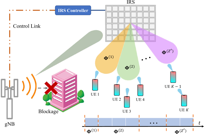
Figure 1: TDMA scheduling for IRS-assisted multi-UE communication.

We consider downlink data transmission for the multi-UE multiple input-multiple output (MIMO) communication system shown in Fig. 1, wherein the transmission from the next generation node base (gNB) to the $K$ UEs is assisted by an IRS.

The gNB and the UEs are equipped with $N_{\rm g}$ and $N_{\rm k}$ antennas, respectively. We assume that the system operates either in the mmWave or the THz bands and that the direct link between the gNB and the UEs is unavailable due to a deep blockage. As a consequence, the gNB transmits signals to the UEs by exploiting the virtual line-of-sight (LoS) link offered by the IRS. Time is divided into frames, each split into $K$ slots, and each UE is served exactly once in a frame.

IRS Model

The $N_{\rm I}$ elements of the IRS act each as an omnidirectional antenna unit that reflects the impinging electromagnetic field, by introducing a tunable phase shift on the baseband-equivalent signal model. We denote with $\phi_{n}=e^{j\theta_{n}}$ the reflection coefficient of the $n$-th IRS element, where $\theta_{n}\in[-\pi,\pi)$ is the induced phase shift. Since recent works argue that continuous-phase shifts are hardly implementable in practice [19], we also consider the case of quantized configurations, in which phase shifts are chosen from a discrete set $\mathcal{P}_{\theta}=\left\{0,\frac{2\pi}{2^{b}},\ldots,\frac{2\pi(2^{b}-1)}{2^{b}}\right\}$, being $b>0$ the number of bits employed to control the quantized phase shifts.

We denote with $\bm{H}(f)\in\mathbb{C}^{N_{\rm I}\times N_{\rm g}}$ the gNB-IRS channel matrix and with $\bm{G}_{k}(f)\in\mathbb{C}^{N_{\rm U}\times N_{\rm I}}$ the channel matrix of the link between the IRS and UE $k$. We consider single-stream transmissions, with $\bm{w}_{{\rm g}_{k}}\in\mathbb{C}^{N_{\rm g}\times 1}$ and $\bm{w}_{{\rm U}_{k}}\in\mathbb{C}^{N_{\rm U}\times 1}$ defined as the beamforming vectors at the gNB and the UE $k$. Let $x_{k}$ be the single-stream signal transmitted by the gNB to UE $k$, the received signal can be then expressed as

$$z_{k}=\bm{w}_{{\rm U}_{k}}^{T}\bm{G}_{k}\bm{\Phi}\bm{H}\bm{w}_{{\rm g}_{k}}x_{k}+\bm{w}_{{\rm U}_{k}}^{T}\bm{n}_{k}.$$ (1)

where $\bm{n}_{k}\in\mathbb{C}^{N_{\rm U}\times 1}$ represents the circularly symmetric complex Gaussian noise vector with zero-mean and variance $\sigma^{2}_{\rm n}$ and $\bm{\Phi}\in\mathbb{C}^{N_{\rm I}\times N_{\rm I}}$ is the IRS configuration, i.e., a diagonal matrix defined as $\bm{\Phi}=\operatorname*{diag}(\phi_{1},\ldots,\phi_{N_{\rm I}})$. Note that specific IRS configurations can be adopted for different UEs. Accordingly, in the following $\bm{\Phi}(k)$ denotes the configuration adopted when UE $k$ is served.

The SNR at UE $k$, with IRS configuration $\bm{\Phi}(k)$, is given by

$$\Gamma_{k}(\bm{\Phi}(k))=\frac{|\bm{w}_{{\rm U}_{k}}^{T}\bm{G}_{k}\bm{\Phi}(k)\bm{H}\bm{w}_{{\rm g}_{k}}|^{2}\sigma_{\bm{x}}^{2}}{|\bm{w}_{{\rm U}_{k}}|^{2}\sigma_{\bm{n}}^{2}},$$ (2)

where $\sigma_{\bm{x}}^{2}$ is the signal power. In general, different IRS configurations should be adopted for each UE to maximize its ownSNR, based on its position in the cell and the channel conditions. The goal of this paper, however, is to limit the IRS reconfigurations as discussed in Section I. Heuristic algorithms able to maximize UEs performance while complying with this requirement will be presented in Section III.

II-A Sum-rate Optimization Problem

The number of IRS reconfigurations may be limited, with the goal of accounting for practical limitations that might arise in realistic deployments.

i reducing the power consumption of the control circuitry and ii taking into account for the limitations incurred by a realistic control channel to the gNB.

On the downside, achieving this goal usually leads to SNR degradation as sub-optimal IRS configurations might be adopted to serve some UEs. To mitigate this effect, we formulate a constrained optimization problem on the average system sum-rate. In the following, the constraint on the maximum number of reconfigurations within a time frame will be referred to as the block-static constraint. For the latter, we assume the following:

1. at most $Z$ IRS reconfigurations can occur within a time frame;

2. the gNB serves the $K$ UEs by partitioning them into $Z$ disjoint subsets $\mathcal{U}_{1},\ldots,\mathcal{U}_{Z}$, with $Z\leq K$;

3. for each UEs subset $\mathcal{U}_{z}$, the same IRS configuration $\bm{\Phi}^{(z)}$ is kept, i.e., $\bm{\Phi}(k)=\bm{\Phi}^{(z)},\forall k\in\mathcal{U}_{z},\forall\,1\leq z\leq Z$.

Let $\mathcal{C}=\{\bm{\Phi}^{(1)},\bm{\Phi}^{(2)},\ldots,\bm{\Phi}^{(Z)}\}$ be the set of IRS configurations corresponding to subsets $\mathcal{U}_{1},\ldots,\mathcal{U}_{Z}$. The average system sum-rate within a time frame is defined as

$$R(\mathcal{U}_{1},\ldots,\mathcal{U}_{Z},\mathcal{C})=\sum_{z=1}^{Z}\sum_{k\in\mathcal{U}_{z}}\log_{2}\left(1+\Gamma_{k}(\bm{\Phi}^{(z)}\right),$$ (3)

where $\Gamma_{k}(\bm{\Phi}^{(z)})$ is the SNR experienced by the $k$-th UE when using the IRS configuration $\bm{\Phi}^{(z)}$.

The optimization problem is thus formulated as

$$\operatorname*{\arg\!\max}_{\begin{subarray}{c}\mathcal{U}_{1},\ldots,\mathcal{U}_{Z},\mathcal{C}\end{subarray}}R(\mathcal{U}_{1},\ldots,\mathcal{U}_{Z},\mathcal{C}),\\$$ (4a)

s.t. $$\theta_{n,z}\in[-\pi,\pi),$$ (4b)

where $\theta_{n,z}=\angle[\bm{\Phi}^{(z)}]_{n,n}$, for $n=1,\ldots,N_{\rm I}$.

III Constrained Sum-rate Optimization

In this section, we provide a heuristic solution to (4). Specifically, we first present two clustering-based approaches to identify and group UEs with a similar optimal IRS configuration. Then, we solve the scheduling problem on the identified clusters with a TDMA approach. We compute the UEs clusters by first estimating the optimal individual IRS configuration, i.e., the configurations leading to the maximum rate when considering only one of the UEs in Sec. III-A. These configurations would solve (4) for $Z=K$, as in this case all UEs are served in a TDMA fashion and with their optimal IRS configuration, denoted as $\bm{\Phi}^{*}(k)$. The phase coefficients of the optimal IRS configuration matrices are then chosen as the initial points of a procedure leveraging arbitrary clustering algorithms in the $N_{\rm I}$-dimensional space, as explained in Sec. III-A. Finally, we propose ad hoc clustering techniques in Sec. III-C.

III-A Individual Optimal IRS Configurations

In MIMO systems, both gNB and UEs adopt properly tuned beamformers to steer the signal towards the spatial direction providing the highest channel gain [20]. For the optimization of the IRS configuration of each individual UE, we adopt a procedure similar to the one presented in [21], focusing on the single-stream transmissions. The optimal beamforming vectors $\bm{w}_{{\rm U}_{k}}$ and $\bm{w}_{{\rm g}_{k}}$ coincide with the singular vectors corresponding to the highest singular value of the wireless channel matrix. In principle, one could thus estimate $\bm{w}_{{\rm U}_{k}}$ and $\bm{w}_{{\rm g}_{k}}$ by applying singular value decomposition on the overall cascade channel matrix

$$\bm{G}_{k}\bm{\Phi}(k)\bm{H}=\bm{U}\bm{\Sigma}\bm{V}^{H},$$ (5)

and obtaining the right and left singular vectors of $\bm{G}_{k}\bm{\Phi}(k)\bm{H}$ as the columns of $\bm{V}$ and $\bm{U}$ and the corresponding singular values as the diagonal entries of $\bm{\Sigma}$. Notice, though, that the cascade channel itself depends on the specific IRS configuration $\bm{\Phi}(k)$, which in our formulation represents one of the optimization variables. Indeed, for fixed $\bm{w}_{{\rm U}_{k}}$ and $\bm{w}_{{\rm g}_{k}}$ we can solve

$$\bm{\Phi}^{*}(k)=\operatorname*{\arg\!\max}_{\begin{subarray}{c}\bm{\Phi}(k)\end{subarray}}\Gamma_{k}(\bm{\Phi}(k)),\quad\text{s.t.}\;\eqref{const_phaseshifters}.$$ (6)

By defining $\bm{v}_{k}=\bm{w}_{{\rm U}_{k}}^{T}\bm{G}$ and $\bm{u}_{k}=\bm{H}\bm{w}_{{\rm g}_{k}}$ and re-writing the received signal power as

$$\left|\bm{v}_{k}\bm{\Phi}(k)\bm{u}_{k}\right|^{2}=\left|\sum_{n=1}^{N_{\rm I}}|[\bm{v}_{k}]_{n}||[\bm{u}_{k}]_{n}|e^{j(\angle[\bm{v}_{k}]_{n}+\theta_{n}+\angle[\bm{u}_{k}]_{n})}\right|^{2}$$ (7)

Then, it is sufficient to observe that the SNR is maximized when the phase shifts introduced by the IRS align the phase-shifts accumulated along the various paths, i.e., when

$$\theta_{n}=-(\angle[\bm{v}_{k}]_{n}+\angle[\bm{u}_{k}]_{n}),\quad\forall n.$$ (8)

To overcome this interdependence between optimal IRS configurations and beamforming vectors we resort to an iterative alternate optimization approach. In particular, we first estimate the optimal beamforming vectors for a given IRS configuration using (5). Then, we plug the derived beamformers into (6) and obtain the corresponding optimal IRS configuration. We repeat this two-step procedure until convergence, which is usually reached in very few iterations. For practical purposes, we assume the convergence is reached when the individual rate achieved in two consecutive iterations differs by less than $10^{-}4$. It must be noted that the number of iterations needed grows with the number of considered antennas and IRS phase shifters. However, with our assumptions, convergence is always reached in less than $10$ iterations.

III-B Clustering-based TDMA scheduling

For an approximated, but close-to-optimal solution to (4), we resort to a clustering-based approach. Our proposed clustering algorithms estimate both the subsets of UEs $\mathcal{U}_{1},\ldots,\mathcal{U}_{Z}$ and the set of respective IRS configurations $\mathcal{C}$. In particular, they operate on the phase vector space. Points to be clustered are identified by the IRS phase shifts vector, i.e.,

$$\left[\angle{\left[\phi\right]_{0}},\ldots,\angle{\left[\phi\right]_{N_{\rm I}}}\right]^{T}=\left[\theta_{0},\ldots,\theta_{N_{\rm I}}\right]^{T},$$ (9)

which maps each IRS configuration $\bm{\Phi}$ to a point in a discrete grid on the continuous space $\left[0,2\pi\right]^{N_{\rm I}}$.

The general clustering-based procedure works as follows:

1. find $\bm{\Phi}^{*}(k),\,\forall k$, i.e., the optimal IRS configurations for each UE,

2. build the UE subsets $\mathcal{U}_{z},\,z=1,\ldots,Z$ by using an arbitrary clustering algorithm,

3. assign $\bm{\Phi}^{(z)}$ to all $k\in\mathcal{U}_{z}$

III-C Capacity-Weighted Clustering

With the aim of maximizing the average system sum rate, we now present the CWC algorithm. The algorithm performs a variable number of iterations until reaching convergence, i.e., until the sum rate difference with the previous step is negligible. Let $\bm{\Phi}_{i}^{(z)}$ be the centroid of the $z$-th cluster at iteration $i$. UEs are initially sorted in decreasing order of achievable SNR. The algorithm selects the $Z$ UEs providing the best performance with their optimal IRS configurations and sets $\bm{\Phi}_{1}^{(z)}=\bm{\Phi}^{*}(k)$, $k=1,\ldots,Z$, $z=1,\ldots,Z$ as the initial centroids. Then, each UE $k>Z$ is assigned to $z^{*}_{k}$, defined as the cluster whose centroid provides the lowest rate difference with respect to the ideal configuration as

$$z^{*}=\operatorname*{\arg\!\min}_{\begin{subarray}{c}z\end{subarray}}\log_{2}\left(\frac{1+\Gamma_{k}(\bm{\Phi}^{*}(k))}{1{+}\Gamma_{k}(\bm{\Phi}_{i}^{(z)})}\right),$$ (10)

where we exploit the well-known logarithm sum property. After the assignments of all the remaining UEs, the coordinates of the centroids need to be updated. At iteration $i+1$ the new centroid of cluster $z$ is computed as the average of all data points belonging to it, weighted by their achievable rate when adopting the centroid as

$$\bm{\Phi}_{i+1}^{(z)}=\frac{\sum_{k\in\mathcal{U}_{z}}\bm{\Phi}^{*}(k)\log_{2}\left(1+\Gamma_{k}(\bm{\Phi}_{i}^{(z)})\right)}{\sum_{k\in\mathcal{U}_{z}}\log_{2}\left(1+\Gamma_{k}(\bm{\Phi}_{i}^{(z)})\right)}.$$ (11)

We repeat this two-step procedure until convergence, which is usually reached in very few iterations, provided that the considered the number of antennas and IRS phase shifters is relatively limited. However, in the case of massive MIMO systems, this procedure could reach high degrees of complexity, thus we also propose another low-complexity clustering algorithm, denoted as one shot CWC (OS-CWC).

III-D One-Shot Capacity-Weighted Clustering

As a low-complexity heuristic clustering solution to problem (4) we propose OS-CWC. As for CWC, UEs are sorted in decreasing order of achievable rate and the $Z$ IRS configurations making the UEs achieving highest rate are chosen as clusters centroids. Then, instead of associating points to clusters and recomputing the coordinates of the centroids at each iteration, the algorithm stops upon the initial association. Therefore, the computed centroids are exactly the optimal configurations of the $Z$ UEs achieving the highest individual rate.

IV Numerical Results

In this section, we assess via simulation the performance of an IRS-aided system with practical constraints. In the 2-D plane, we consider a urban micro-cell (UMi) cell [22], with the gNB placed at the origin. The coverage area is delimited by the 120° field-of-view (FoV) of the gNB and the cell radius, according to the specification, is fixed to $167$ m. $K=100$ UEs are uniformly deployed UEs within the cell coverage area, to be served in the downlink by the gNB assisted by anIRS with $(x,y)$ coordinates of $(75,100)$ m. We remark that the direct links between gNB and all UEs are assumed to exhibit severe attenuation due to blockage, thus being not exploitable for data transmission. The gNB is equipped with an $8\times 8$ uniform planar array (UPA) antenna panel ($N_{\rm g}=64$) and all UEs with uniform linear arrays (ULAs) of $N_{\rm U}=2$ antennas. For the IRS size, if not specified in the following, we adopt a $40\times 80$ reflective panel ($N_{\rm I}=3200$).The transmission power at the gNB is set to $33$ dBm, while the noise power spectral density at the receivers is $-174$ dBm/Hz. Finally, the total system bandwidth is $100$ MHz. We consider the 3rd Generation Partnership Project (3GPP) TR 38.901 spatial channel model [22], wherein channel matrices are computed based on the superposition of different clusters of rays, each one arriving (departing) to (from) the antenna arrays with specific angles and powers. Finally, we assume that the gNB-IRS link exhibits a LoS path, while the IRS-UE links are in non-line-of-sight (NLoS) conditions.

IV-A Clustering Algorithms Benchmark

The performance of our proposed scheduling strategies, i.e., CWC and OS-CWC, is compared to that achieved by the following traditional clustering algorithms.

K-means (KM)

KM clustering [23] aims at finding $Z$ disjoint clusters minimizing the within-cluster sum of squares. To perform KM clustering, we here consider the well-known Lloyd algorithm [24], which randomly selects $Z$ points in the space of phase vectors as the initial centroids. Then, it assigns each data point to the closest centroid, i.e., the one with the smallest squared Euclidean distance. The set of centroids is then re-computed as the average of all data points that belong to each cluster. These steps are repeated until either convergence is met, or a maximum number of iterations (here fixed to $100$) is reached.

Agglomerative hierarchical clustering (HC)

The agglomerative HC [25] is a clustering technique that partitions a set of data points into disjoint clusters by iteratively merging points into clusters, until the target number of partitions is met. In particular, the clusters are initialized as the optimal phase vectors, which thus act as the respective centroids. Then, the average Euclidean distance between all pairs of data points in any two clusters is evaluated. The closest pair of clusters is then merged into a new single cluster whose centroid is computed as the average of all its data points. The procedure is repeated until the number of clusters is equal to $Z$.

Finally, we also consider two bounds on the scheduling performance. The former is an achievable lower bound based on random clustering, where the UEs are randomly partitioned into $Z$ clusters, and each cluster centroid is computed as the average of all data points in the cluster. Thus, it is reasonable to expect that any sensible algorithm performs better than this trivial solution. The latter, denoted as unclustered scheduling, assumes that all UEs are served with their optimal IRS configuration. This is clearly an upper bound that violates the constraint on the minimum reconfiguration period, but can be regarded as the limit case when $Z=K$, thus all UEs belong to a cluster with cardinality one.

IV-B Scheduling Performance

Figure 2: Average sum-rate as a function of the maximum number of clusters allowed $Z$.

Fig. 2 shows the average rate per slot as a function of the number of clusters $Z$. It can be observed that all the scheduling policies are increasing with respect to $Z$, and they converge to the unclustered policy. This is motivated by the fact that a higher number of clusters leads to a smaller intra-cluster average distance, which eventually becomes $0$ for all clusters when $Z=K$. In turn, this metric relates to “how far" a given UE ideal configuration is from the centroid, i.e., the configuration which will be used by all the UEs which belong to the cluster. Among the considered clustering policies, CWC and OS-CWC provide the highest sum-rate thanks to the bias towards UEs which achieve a good signal quality when served using their optimal IRS configuration. Finally, the gap between CWC and OS-CWC is negligible, which suggests that UEs’ ideal configurations belong to well-defined isolated regions of the phase-vector space. As a consequence, a single iteration in the clustering procedure is enough to achieve good performance, which implies a good scalability of the proposed technique.

Figure 3: Average sum-rate as a function of the number of IRS radiating elements.

Fig. 3 depicts the impact of the number of IRS radiating elements on the system performance, when considering the CWC policy. As expected, the achievable rate increases as we use bigger IRSs, regardless of the number of clusters. Furthermore, it can be noted that varying the number of reflecting elements has an impact on the number of clusters that are needed to provide the maximum achievable rate as well. Indeed, the number of possible IRS configurations increases as we consider arrays featuring additional antenna elements, as the reflected beams get progressively narrower. In turn, this decreases the likelihood of UEs exhibiting the same (or similar) ideal configurations. We remark that our proposed solution is able to almost provide the optimal rate with as few as $20$ clusters for small-sized IRSs, i.e., featuring $10\times 20$ or $20\times 40$ arrays.

Figure 4: Average sum-rate as a function of the IRS phase-shifters quantization resolution.

Finally, Fig.4 shows the average sum-rate as a function of the maximum number of clusters computed by the CWC algorithm, for different numbers of bits $b$ used for the IRS phase shifts quantization. Results show that considering non-ideal phase-shifters leads to a considerable rate degradation when UEs are in this particular SNR region. In particular, considering a $b=1$ quantization at the IRS incurs up to a $60\%$ reduction in the achieved rate with respect to the continuous case. Instead, such a gap is not as dramatic when considering higher resolution phase-shifters.

V Conclusions

In this paper, we have considered a MIMO communication system, in which a gNB that serves multiple UEs experiences a deep blockage and is thus assisted by an IRS possibly having practical constraints on his configuration period. We have considered a TDMA scheduling of downlink transmissions, and we have formulated an optimization problem that aims at maximizing the average system rate subject to a fixed number of IRS reconfigurations per radio time frame. We have mitigated the performance degradation caused by such a limitation by proposing clustering-based scheduling policies, which group UEs with similar ideal IRS configurations. This allows to reduce the number of configurations as all the UEs belonging to a specific cluster are served with the same IRS parameters.

We have analyzed the sum-rate performance of the proposed clustering-based approaches and highlighted the benefit of adopting a rate-driven clustering with respect to the traditional KM or HC algorithms. The obtained results show that our approach is effective in guaranteeing up to $85$% of the throughput obtained by an ideal deployment (with no reconfiguration constraints) while providing a $50$% reduction in the number of IRS reconfigurations.

References

- [1] 3GPP, “NR; Base Station (BS) radio transmission and reception,” TS 38.104 (Rel. 17), 2022.
- [2] M. Polese, J. M. Jornet, T. Melodia, and M. Zorzi, “Toward end-to-end, full-stack 6G terahertz networks,” IEEE Commun. Mag., vol. 58, no. 11, pp. 48–54, Nov. 2020.
- [3] S. Rangan, T. S. Rappaport, and E. Erkip, “Millimeter-wave cellular wireless networks: Potentials and challenges,” Proc. IEEE, vol. 102, no. 3, pp. 366–385, Mar. 2014.
- [4] D. López-Pérez, M. Ding, H. Claussen, and A. H. Jafari, “Towards 1 Gbps/UE in cellular systems: Understanding ultra-dense small cell deployments,” IEEE Commun. Surveys Tuts., vol. 17, no. 4, pp. 2078–2101, Jun. 2015.
- [5] A. Chaoub, M. Giordani, B. Lall, V. Bhatia, A. Kliks, L. Mendes, K. Rabie, H. Saarnisaari, A. Singhal, N. Zhang et al., “6G for bridging the digital divide: Wireless connectivity to remote areas,” IEEE Wireless Commun., vol. 29, no. 1, pp. 160–168, Jul. 2021.
- [6] R. Flamini, D. De Donno, J. Gambini, F. Giuppi, C. Mazzucco, A. Milani, and L. Resteghini, “Towards a heterogeneous smart electromagnetic environment for millimeter-wave communications: An industrial viewpoint,” IEEE Trans. Antennas Propag., Feb. 2022.
- [7] E. Björnson, Ö. Özdogan, and E. G. Larsson, “Intelligent reflecting surface versus decode-and-forward: How large surfaces are needed to beat relaying?” IEEE Commun. Lett., vol. 9, no. 2, pp. 244–248, Oct. 2019.
- [8] Q. Wu and R. Zhang, “Towards smart and reconfigurable environment: Intelligent reflecting surface aided wireless network,” IEEE Commun. Mag., vol. 58, no. 1, pp. 106–112, 2020.
- [9] S. Abeywickrama, R. Zhang, Q. Wu, and C. Yuen, “Intelligent reflecting surface: Practical phase shift model and beamforming optimization,” IEEE Trans. Commun., vol. 68, no. 9, pp. 5849–5863, Jun. 2020.
- [10] Q. Wu and R. Zhang, “Intelligent reflecting surface enhanced wireless network via joint active and passive beamforming,” IEEE Trans. Wireless Commun., vol. 18, no. 11, pp. 5394–5409, Aug. 2019.
- [11] M. Pagin, M. Giordani, A. A. Gargari, A. Rech, F. Moretto, S. Tomasin, J. Gambini, and M. Zorzi, “End-to-end simulation of 5G networks assisted by IRS and AF relays,” in Proc. IEEE MedComNet, 2022, pp. 150–157.
- [12] R. Liu, Q. Wu, M. Di Renzo, and Y. Yuan, “A path to smart radio environments: An industrial viewpoint on reconfigurable intelligent surfaces,” IEEE Wireless Commun., vol. 29, no. 1, pp. 202–208, 2022.
- [13] C. Liaskos, S. Nie, A. Tsioliaridou, A. Pitsillides, S. Ioannidis, and I. Akyildiz, “Realizing wireless communication through software-defined hypersurface environments,” in Proc. IEEE WoWMoM, 2018, pp. 14–15.
- [14] M. Rossanese, P. Mursia, A. Garcia-Saavedra, V. Sciancalepore, A. Asadi, and X. Costa-Perez, “Designing, building, and characterizing RF switch-based reconfigurable intelligent surfaces,” arXiv preprint arXiv:2207.07121, 2022.
- [15] F. Guidolin, A. Orsino, L. Badia, and M. Zorzi, “Statistical analysis of non orthogonal spectrum sharing and scheduling strategies in next generation mobile networks,” in Proc. IEEE IWCMC, 2013, pp. 680–685.
- [16] A. Marotta, D. Cassioli, C. Antonelli, K. Kondepu, and L. Valcarenghi, “Network solutions for CoMP coordinated scheduling,” IEEE Access, vol. 7, pp. 176 624–176 633, 2019.
- [17] S. Bassoy, M. Jaber, M. A. Imran, and P. Xiao, “Load aware self-organising user-centric dynamic CoMP clustering for 5G networks,” IEEE Access, vol. 4, pp. 2895–2906, 2016.
- [18] F. Guidolin, L. Badia, and M. Zorzi, “A distributed clustering algorithm for coordinated multipoint in LTE networks,” IEEE Wireless Commun. Lett., vol. 3, no. 5, pp. 517–520, 2014.
- [19] X. Tan, Z. Sun, D. Koutsonikolas, and J. M. Jornet, “Enabling indoor mobile millimeter-wave networks based on smart reflect-arrays,” in Proc. IEEE Infocom, Apr. 2018.
- [20] N. Benvenuto, G. Cherubini, and S. Tomasin, Algorithms for communications systems and their applications. John Wiley & Sons, 2021.
- [21] X. Qian, M. Di Renzo, V. Sciancalepore, and X. Costa-Pérez, “Joint optimization of reconfigurable intelligent surfaces and dynamic metasurface antennas for massive MIMO communications,” in Proc. IEEE SAM workshop, 2022, pp. 450–454.
- [22] 3GPP, “Study on channel model for frequencies from 0.5 to 100 GHz,” 3rd Generation Partnership Project (3GPP), Technical Report (TR) 38.901, Jan. 2020, version 16.1.0.
- [23] L. Rokach and O. Maimon, “Clustering methods,” in Data mining and knowledge discovery handbook. Springer, 2005, pp. 321–352.
- [24] S. Lloyd, “Least squares quantization in PCM,” IEEE Trans. Inf. Theory, vol. 28, no. 2, pp. 129–137, Mar. 1982.
- [25] F. Murtagh and P. Contreras, “Algorithms for hierarchical clustering: an overview,” Wiley Interdisciplinary Reviews: Data Mining and Knowledge Discovery, vol. 2, no. 1, pp. 86–97, 2012.