MIDIS: Strong (H$\beta$+[O III]) and H$\alpha$ emitters at redshift $z\simeq 7-8$ unveiled with JWST/NIRCam and MIRI imaging in the Hubble eXtreme Deep Field (XDF)

Abstract

We make use of JWST medium and broad-band NIRCam imaging, along with ultra-deep MIRI $5.6\rm\mu m$ imaging, in the Hubble eXtreme Deep Field (XDF) to identify prominent line emitters at $z\simeq 7-8$. Out of a total of 58 galaxies at $z\simeq 7-8$, we find 18 robust candidates ($\simeq$31%) for (H$\beta$ + [O III]) emitters, based on their enhanced fluxes in the F430M and F444W filters, with EW₀(H$\beta$ +[O III]) $\simeq 87-2100\,\rm\AA$. Among these emitters, 16 lie in the MIRI coverage area and 12 exhibit a clear flux excess at $5.6\,\rm\mu m$, indicating the simultaneous presence of a prominent H$\alpha$ emission line with EW₀(H$\alpha$) $\simeq 200-3000\,\rm\AA$. This is the first time that H$\alpha$ emission can be detected in individual galaxies at $z>7$. The H$\alpha$ line, when present, allows us to separate the contributions of H$\beta$ and [O III] to the (H$\beta$ +[O III]) complex, and derive H$\alpha$-based star formation rates (SFRs). We find that in most cases [O III]/H$\beta>1$. Instead, two galaxies have [O III]/H$\beta<1$, indicating that the NIRCam flux excess is mainly driven by H$\beta$. This could potentially imply extremely low metallicities. The most prominent line emitters are very young starbursts or galaxies on their way to/from the starburst cloud. They make for a cosmic SFR density $\rm log_{10}(\rho_{SFR_{H\alpha}}/(\rm M_{\odot}\,yr^{-1}\,Mpc^{-3}))\simeq-2.35$, which is about a quarter of the total value ($\rm log_{10}(\rho_{SFR_{tot}}/(\rm M_{\odot}\,yr^{-1}\,Mpc^{-3}))\simeq-1.76$) at $z\simeq 7-8$. Therefore, the strong H$\alpha$ emitters likely had a significant role in reionization.

.

1 Introduction

Quantifying the presence and properties of galaxies present at the Epoch of Reionization (EoR) is necessary to explain how this major phase transition of the Universe has occurred. Over the past decade, many studies have focused on this topic, but a few important problems complicated the selection of galaxies at this cosmic time. The increasing intergalactic medium absorption with redshift means that basically all photons blueward of the Lyman-$\alpha$ spectral line at $\lambda_{\rm rest}=1216\,\rm\AA$ cannot reach us. Indeed, it is well known that the incidence of Lyman-$\alpha$ emitters (LAEs) has a sharp drop at $z>7$ (e.g., Fontana et al., 2010; Ono et al., 2012; Caruana et al., 2014; Pentericci et al., 2014). Therefore, other emission lines at longer wavelengths must be considered to facilitate the search of galaxies at such high redshifts (e.g., Stark et al., 2015).

However, detecting the optical emission from atomic transitions at $z>7$ was virtually impossible until now, given the lack of sufficiently sensitive near and mid-infrared observatories. The recent advent of the JWST is now radically changing this situation by offering, for the first time, sensitive imaging and spectroscopy at such long wavelengths. Indeed, in the first six months of operations, JWST has enabled a number of studies of $z>7$ galaxies, particularly on their line emission properties (e.g., Arellano-Córdova et al., 2022; Langeroodi et al., 2022; Morishita & Stiavelli, 2022; Trump et al., 2022; Wang et al., 2022; Williams et al., 2022).

With imaging, the search of line emitters is facilitated by the fact that the rest-frame equivalent widths (EWs₀) of some of the main optical emission lines appear to increase, on average, with redshift (e.g., De Barros et al., 2019; Matthee et al., 2022). This has allowed for the search of prominent line emitters at intermediate and high redshifts, by identifying galaxies with photometric excess in narrow-band images (e.g., Khostovan et al., 2016) and even broad-band images (e.g., Faisst et al., 2016; Roberts-Borsani et al., 2016; Smit et al., 2016; Caputi et al., 2017). This trend of increasing EWs₀ with redshift is indicative of an evolution in the galaxy average specific star formation rates (sSFR) (e.g., Faisst et al., 2016; Tang et al., 2019), as well as the conditions of their interstellar medium (ISM) (e.g., Schaerer & de Barros, 2009).

At $z>7$ both the H$\beta\,\lambda 4861\,\rm\AA$ and [O III] $\lambda\lambda 4959,5007$ emission lines are shifted into the JWST’s Near-IR Camera (NIRCam; Rieke et al., 2005) wavelength range, making that these lines together can produce a flux excess in the NIRCam filters at $\simeq 4-5\,\rm\mu m$. In turn, the (H$\alpha\,\lambda 6563$ + [NII] $\lambda\lambda 6548,6583$ + [SII] $\lambda\lambda 6716,6730$) complex appears in the Mid-Infrared Instrument (MIRI; Rieke et al., 2015; Wright et al., 2015) wavelength domain at observed $>5\,\rm\mu m$.

In this paper, we make use of publicly available NIRCam images in the Hubble eXtreme Deep Field (XDF) to search for (H$\beta$ + [O III]) emitters at $z\simeq 7-8$. In most of this field, we also benefit from ultra-deep MIRI $5.6\,\rm\mu m$ imaging, which we analyse to search for the presence of H$\alpha$ emission in the same galaxies. This is the first time that the H$\alpha$ line can be detected and quantified in individual galaxies at $z>7$. This paper is organised as follows: in §2 we describe the datasets, photometric measurements and spectral energy distribution (SED) fitting that allows us to select galaxies at $z\simeq 7-8$. In §3 we explain our methodology to identify strong (H$\beta$ + [O III]) and H$\alpha$ emitters amongst these galaxies. We present all our results in §4 and our conclusions in §5. Throughout this paper, we consider a cosmology with $\rm H_{0}=70\,{\rm km\,s^{-1}Mpc^{-1}}$, $\rm\Omega_{M}=0.3$ and $\rm\Omega_{\Lambda}=0.7$. All magnitudes are total and refer to the AB system (Oke & Gunn, 1983). A Chabrier (2003) initial mass function (IMF) is assumed.

2 Datasets, Photometry and SED fitting

2.1 Datasets

The Hubble XDF (Illingworth et al., 2013, see Fig. 1) is a small field of the sky with the deepest Hubble Space Telescope (HST) observations ever taken since this telescope started operations more than thirty years ago. This field has been the main window to study the early Universe before the JWST advent, with numerous works scientifically exploiting its unique possibilities. Now in the JWST era, the HST data in the XDF and surroundings are being enhanced with deep imaging and spectroscopy obtained with JWST/NIRCam and MIRI, extending the wavelength coverage of high spatial-resolution observations to the mid-infrared.

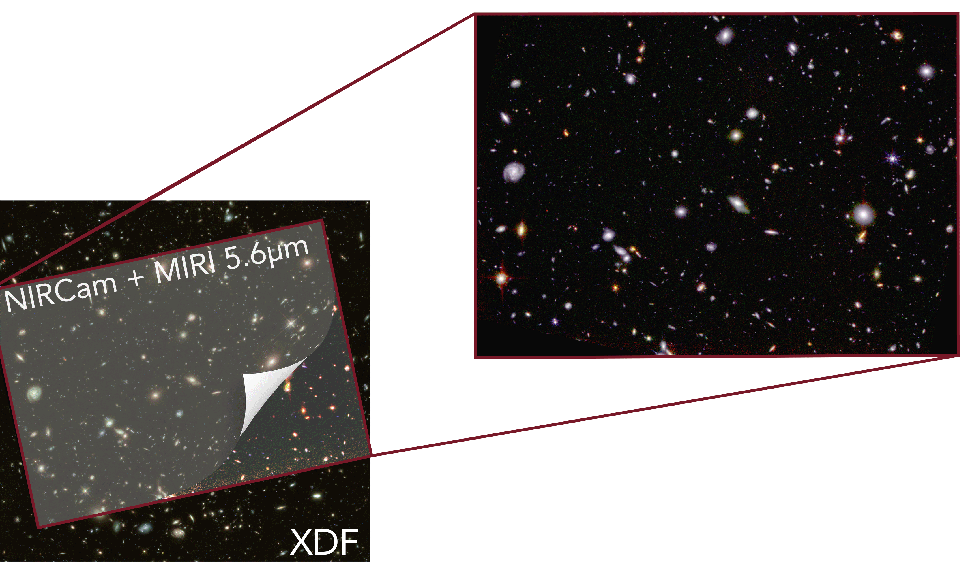
Figure 1: An RGB mosaic of the Hubble eXtreme Ultra Deep Field. This image has been obtained by exploiting the HST and JWST images currently available in this field. In particular, the background image has been obtained by combining HST and JWST/NIRCam filters. The zoom-in shows the region covered by MIRI/F560W. In this case, to create the RGB image, we adopted the JWST filters only where R: F560W; G: F430M, F444W, F460M, and F480M; B: F182M and F210M. The RGB images have been produced using the software Trilogy (Coe, 2015).

2.1.1 JWST/NIRCam

In this work, we made use of the recent JWST/NIRCam images collected by Williams et al. (2023) in a General Observers Cycle-1 program across the HUDF (PID: 1963; PI: Christina C. Williams). Observations have been taken in 5 JWST/NIRCam medium bands: F182M, F210M, F430M, F460M, and F480M. In particular, 7.8 hours of the total integration time have been dedicated to F182M, F210M, and F480M. Instead, only 3.8 hours of observations have been collected for F430M and F460M. In order to complement these datasets, we also made use of the imaging data taken as part of The First Reionization Epoch Spectroscopic COmplete Survey (Oesch et al., 2021, 2023, FRESCO) (PID: 1895; PI: Pascal Oesch). On the one hand, this GO program allowed us to add more depth to F182M and F210M, on the other hand it gave us the opportunity to include F444W in our analysis.

All JWST/NIRCam images have been reduced by adopting a modified version of the official JWST pipeline (based on jwst 1.8.2 and Calibration Reference Data System pipeline mapping (CRDS; pmap) 1018)). More detailed information about the reference files is available on the official STScI/CRDS website.

Compared to the official JWST pipeline, our version includes different procedures, following some of the ideas presented in Bagley et al. (2022), to deal with the unresolved problems that still affect the official software. In our data reduction, we minimized the impact of the so-called “snowballs”, the 1/f noise, the “wisps”, and the residual cosmic rays. After reducing all the JWST/NIRCam images from Williams’s and FRESCO programs, we drizzled all the NIRCam calibrated files to 0.03″/pixel, as the final pixel scale we adopted in this work. All the final images have been aligned to the Hubble Legacy Fields (HLF) catalogue.

As a sanity check, we compared the photometry for the brightest sources ($<$ 24 mag) in all the NIRCam filters. To do that, we produced two versions of our final images, with and without the extra steps we employed in our modified version of the official pipeline. Then, we extracted the sources by using the software Source Extractor (SExtractor, Bertin & Arnouts, 1996) and compared their photometry. This test demonstrated that our extra steps do not introduce any kind of systematic effect in the photometry.

2.1.2 JWST/MIRI

We complemented the JWST/NIRCam observations with the MIRI $5.6\mu$m imaging from the JWST Guaranteed Time Observations (GTO) program: MIRI Deep Imaging Survey (MIDIS) (PID: 1283, PI: Göran Östlin). The MIRI observations were carried out in December 2022 and targeted with the broad-band filter F560W the HUDF for a total amount of 50 hours ($\approx 41$ hours on-source), covering an area of about 4.7 arcmin². By reaching a median depth of 29.15 mag ($5\sigma$, r = 0.15″), this set of observations represents the deepest imaging available at $5.6\mu$m to date. A complete description of the data collection and reduction, as well as the source statistics on these $5.6\mu$m images, will be presented by Östlin et al. (2023, in prep.). Here we only summarize the basic information of this data processing.

As in the case of the NIRCam imaging, we adopted a modified version of the official JWST pipeline to reduce the MIRI data. In fact, the final products that can be obtained by running the JWST pipeline are still affected by strong patterns (e.g., vertical striping and background gradients) that impact the scientific quality of the images (e.g., Iani et al., 2022). To overcome these problems, we added to the pipeline some extra steps at the end of stages 2 and 3 that allowed us to significantly mitigate the intensity of the striping, the background inhomogeneities as well as the noise of the output image. A comparison between the F560W magnitude of the brightest galaxies ($<24$ mag) measured in MIRI images obtained with and without the extra steps ensured that our modified version of the pipeline did not introduce any systematic offset.

Finally, we drizzled the final MIRI image to the same pixel scale adopted for the JWST/NIRCam images and registered its astrometry to the HLF catalogue.

2.1.3 Ancillary HST data

We obtained all of HST images over the HUDF from the Hubble Legacy Field GOODS-S (HLF-GOODS-S). The HLF-GOODS-S provides 13 HST bands covering a wide range of wavelengths (0.2$\mu$m - 1.6$\mu$m), from the UV (WFC3/UVIS F225W, F275W, and F336W filters), optical (ACS/WFC F435W, F606W, F775W, F814W and F850LP filters), to near-infrared (WFC3/IR F098M, F105W, F125W, F140W and F160W filters). See Whitaker et al. (2019) for more detailed information on these observations.

2.2 Photometric Analysis

We used the software SExtractor to detect the sources and measure their photometry in all the 20 filters available from HST and JWST, covering a wide range of wavelengths (0.2$\mu$m $-$ 5.6$\mu$m). We used SExtractor in dual-image mode adopting a super-detection image that we created by combining photometric information from different bands. In order to maximize the number of the detected sources, we opted to use a hot-mode extraction, as presented in Galametz et al. (2013) which is well suited to find very faint sources.

We combined aperture photometry, adopting circular apertures (i.e., MAG_APER) of 0.5”-diameter, and Kron apertures (i.e., MAG_AUTO, Kron, 1980) following the same prescription we adopted in Rinaldi et al. (2022, see section 3.2). We chose a circular-aperture flux over a Kron flux when the sources were fainter than a given magnitude. In this case, since we were dealing with very deep images, we decided to consider mag = 27 as our faint limit for the Kron aperture. This final decision has been taken after several tests we performed with the HST photometry, comparing our fluxes with the HLF photometric catalogue from Whitaker et al. (2019). We corrected the aperture fluxes to the total. For HST, these corrections are well known. For JWST, instead, we estimated the aperture corrections using the software WebbPSF.

Moreover, we adopted a minimum error of 0.05 mag for all the HST photometry because SExtractor typically underestimates photometric errors (e.g., Sonnett et al., 2013). We decided to adopt this minimum error value for the JWST images as well to account for possible uncertainties in the NIRCam and MIRI flux calibrations.

Finally, all our fluxes have been corrected for Galactic extinction. Those values have been estimated adopting a python package called dustmap. As a sanity check, we compared the correction factors for the HST filters with Schlafly & Finkbeiner (2011), finding an excellent agreement with the values we can recover following their prescription, as expected.

2.3 SED fitting

We performed the SED fitting and derived the properties of our sources by making use of the code LePHARE (Arnouts & Ilbert, 2011). We constructed the libraries for LePHARE by adopting the same configuration we used in Rinaldi et al. (2022, see section 4). Briefly, we considered the stellar population synthesis (SPS) models proposed by Bruzual & Charlot (2003, hereafter BC03), based on the Chabrier IMF (Chabrier, 2003). We made use of two different star formation histories (SFHs): a standard exponentially declining SFH (known as “$\tau$-model”) and an instantaneous burst adopting a simple stellar population (SSP) model. In particular, we adopted two distinct metallicity values, a solar metallicity (Z_⊙ = 0.02) and a fifth of solar metallicity (Z = 0.2Z_⊙ = 0.004). Moreover, to take into account the strong contribution from the nebular emission lines that can occur at very young ages, we also considered STARBURST99 templates (Leitherer et al., 1999, hereafter SB99) for young galaxies (age $\leq 10^{7}\,\rm yr$) with constant star formation histories. We considered the Calzetti et al. (2000) reddening law in combination with Leitherer et al. (2002) to better constrain wavelengths below 912 Å. In particular, we adopted the following color excess values: $0\leq E(B-V)\leq 1.5$, with a step of 0.1. We also decided to run LePHARE between $z=0$ and $z=20$, by considering the following steps: $\Delta z=0.04$ between $z=0$ and $z=6$ and $\Delta z=0.1$ between $z=6$ and $z=20$ (291 steps in total). We summarize the parameters we adopted to perform the SED fitting in Table 1.

Table 1: The parameters we used to perform the SED fitting with LePHARE by adopting BC03 and SB99 models.

Parameter
Templates	Bruzual & Charlot (2003)	Leitherer et al. (1999)
$e-$folding time ($\tau$)	0.01 - 15 (8 steps) + SSP	constant SFH
Metallicty (Z)	0.004; 0.02 ($=$Z⊙)	0.008; 0.001
Age (Gyr)	0.001 - 13.5 (49 steps)	0.001 - 0.1 (6 steps)
	Common values
Extinction laws	Calzetti et al. (2000) + Leitherer et al. (2002)
E(B-V)	0-1.5 (16 steps)
IMF	Chabrier (2003)
Redshift	0-20 (291 steps)
Emission lines	Yes
Cosmology (H0, $\mathrm{\Omega_{0}}$, $\mathrm{\Lambda_{0}}$)	70, 0.3, 0.7

Note. — For the run with SB99 models, we used the same configuration as for the BC03 models for the extinction law, E(B-V), IMF, redshift interval, and cosmology. Moreover, for the run with SB99, we opted for only 6 steps in age because nebular emission lines only matter for very young ages.

We estimated upper limits for each source that SExtractor was not able to detect. To do that, around each source, we placed random circular apertures (0.5″-diameter) to estimate the background r.m.s. (1$\sigma$). For LePHARE, we opted to use the 3$\sigma$ upper limit for the flux in those filters where we did not have a detection. Finally, for all those sources for which we did not have any photometric information (e.g., the MIRI/F560W and NIRCam coverage areas are different), we simply ignored those filters during the SED fitting (i.e., we used $-99$ as input flux in LePHARE).

3 Selection of strong (H$\beta$+[O III]) and H$\alpha$ emitters at $z\simeq 7-8$

LePHARE returns the best-fit SED and derived parameters for each source. We performed two different runs with LePHARE, one adopting BC03 models only and the other one adopting SB99 models only. Therefore, we created the final catalogue choosing for each source the best $\chi_{\nu}^{2}$ between the BC03 and SB99 solutions. Finally, we cleaned our catalogue of possible stars. To do so, we first cross-matched our catalogue with Gaia Data Release 3 (Babusiaux et al., 2022, GAIA DR3). Then, we looked at the stellarity parameter (i.e., CLASS_STAR) we have from SExtractor. In particular, we applied the same criterion adopted in Caputi et al. (2011, Section 3.1). We removed all those sources that have CLASS_STAR $>$ 0.8 and occupy the stellar locus in the (F435W $-$ F125W) versus (F125W $-$ F444W) colour$-$colour diagram. In total, less than $\simeq$ 1% sources have been discarded from our full catalogue because they have been classified as stars (8 of them have been identified in GAIA DR3).

Since our goal is to look for potential (H$\beta$ + [O III]) and (H$\alpha$+[NII]+[SII]) emitters in the XDF at z $\simeq 7-8$, we only focused on those sources for which the best photometric redshift falls in that redshift range.

For each candidate, we created postage stamps to make a careful visual inspection in order to exclude all those galaxies that either fall on stellar spikes or are heavily contaminated by the light of the nearby sources. After this visual inspection, we were left with 58 robust galaxy candidates at $z\simeq 7-8$.

Among these sources, we searched for (H$\beta$ + [O III]) and H$\alpha$ emitters. We first analysed if they show a flux excess in the following three bands: NIRCam/F430M, NIRCam/F444W, and MIRI/F560W. The first two filters have been used to look at the flux enhancement produced by (H$\beta$ + [O III]). In turn, MIRI/F560W has been used to look at the flux excess produced by H$\alpha$.

To convert the flux excess into an EW₀ we followed the canonical approach described by Mármol-Queraltó et al. (2016). Following that procedure, we know that:

$$\mathrm{EW_{0}=\frac{W_{rec}}{1+z}(10^{(-0.4\Delta mag)}-1)},$$ (1)

where W_rec is the rectangular width of the filter containing the emission line in question, in our case (H$\beta$ + [O III]) or H$\alpha$, and $\Delta$mag is the difference between the observed magnitude in that filter and the synthetic magnitude from the SED fitting (i.e., $\Delta$mag = m_obs - m_syn) that we adopted as a proxy for the continuum emission.

Therefore, to estimate the flux excess, we assumed that the continuum flux was well described by the synthetic NIRCam/F460M obtained from the best-fit template for each galaxy. In particular, we selected all those sources for which $\rm|mag_{obs}(F460M)-mag_{syn}(F460M)|\leq 2\;\times$ mag_err(F460M), where mag_obs and mag_syn are the observed and best-fit synthetic magnitudes, respectively. This condition ensures that the continuum at 4.6$\mu$m can be considered flat within the error bars. We also double-checked if this condition was satisfied in NIRCam/F480M.

Once we selected all those sources that survive the condition described above, we estimated the flux excess in the following way: $\rm\Delta mag=(mag_{X}-mag_{cont}$), where $\rm mag_{X}$ represents the magnitude in one of the filters we chose to select (H$\beta$+[O III]) or H$\alpha$, and $\rm mag_{cont}$ refers to $\rm F460M_{syn}$. We highlight that this selection is purely based on the photometric excess we considered above. None of our derivations is based on emission lines modelled by LePHARE. For a conservative approach, we only considered those galaxies for which the flux excess with respect to the stellar continuum satisfies the following condition: $\Delta$mag $<$ $-0.2$. Note that a $\Delta$mag $=-0.2$ in NIRCam/F430M corresponds to a EW₀ $\simeq 58\,\rm\AA$ at $z=7$, while in NIRCam/F444W it would imply an EW₀ $\simeq 270\,\rm\AA$. For MIRI/F560W, the same $\Delta$mag would correspond to an EW₀ $\simeq 239\,\rm\AA$ at the same redshift.

We inspected again the postage stamps of the 58 possible candidates, after estimating the flux excess in each band (NIRCam/F430M, NIRCam/F444W, and MIRI/F560W), to make a cross-match between the values we got for $\Delta$mag and the visual inspection of the sources themselves. We also examined the best-fit SED for each galaxy. This safely allowed us to conclude that 18 sources can be securely classified as (H$\beta$ + [O III]) emitters. These emitters constitute $\simeq 31\%$ of our total galaxy sample at $z\simeq 7-8$ (see Fig. 2 where we show the multiwavelength images of an example source). The derived EW₀ values cover a wide range that goes from a minimum of $87.5^{+30}_{-27}\,\rm\AA$ to a maximum value of $2140.4^{+970}_{-154}\,\rm\AA$, with a median $\left\langle\rm EW_{0}\right\rangle\simeq 943_{-194}^{+737}\,\rm\AA$ (lower and upper errors refer to the 16th and 84th percentiles). This value is higher, but still marginally consistent with the error bars, than that derived by Labbé et al. (2013) from Spitzer Space Telescope observations of bright $z\simeq 8$ galaxy candidates. Out of the 18 (H$\beta$ + [O III]) emitters, $83\%$ have a best-fit SED with sub-solar ($\rm 0.2\,Z_{\odot}$) metallicity and the remaining $\simeq 17\%$ with solar ($\rm Z_{\odot}$) metallicity.

Among the 18 (H$\beta$ + [O III]) emitters at $z\simeq 7-8$, a total of 16 lie on the ultra-deep MIRI $5.6\,\rm\mu m$ coverage field. Out of them, 12 show a significant $5.6\,\rm\mu m$ flux excess with respect to the continuum (as defined above), which we interpret as the presence of the (H$\alpha$+[NII]+[SII]) line complex at $z\simeq 7-8$. To obtain the net value of the H$\alpha$ EW₀, we applied the correction recipes provided by Anders & Fritze-v. Alvensleben (2003), as follows: $f$(H$\alpha$) = 0.63$f$(H$\alpha$ + [NII] + [SII]) for a solar metallicity, and $f$(H$\alpha$) = 0.81$f$(H$\alpha$ + [NII] + [SII]) for a $\rm 0.2\,Z_{\odot}$ metallicity. Note that with this procedure we are assuming that the stellar and gas metallicities are similar in these galaxies.

We also compared the derived stellar properties from the SED-fitting between the (H$\beta$ + [O III]) and H$\alpha$ emitters and non-emitters. Performing the two-sample Kolmogorov-Smirnov test, we do not find any significant difference between the two samples in terms of ages, E(B-V), metallicity, and stellar mass. Regarding the SFR_best distributions, we see a difference between the two populations (SFR_best for the emitters tend to be higher than SFR_best for the non-emitters) that might reflect the fact that we are looking at strong emitters (i.e., SFR is higher). We show these distributions in Fig. 3.

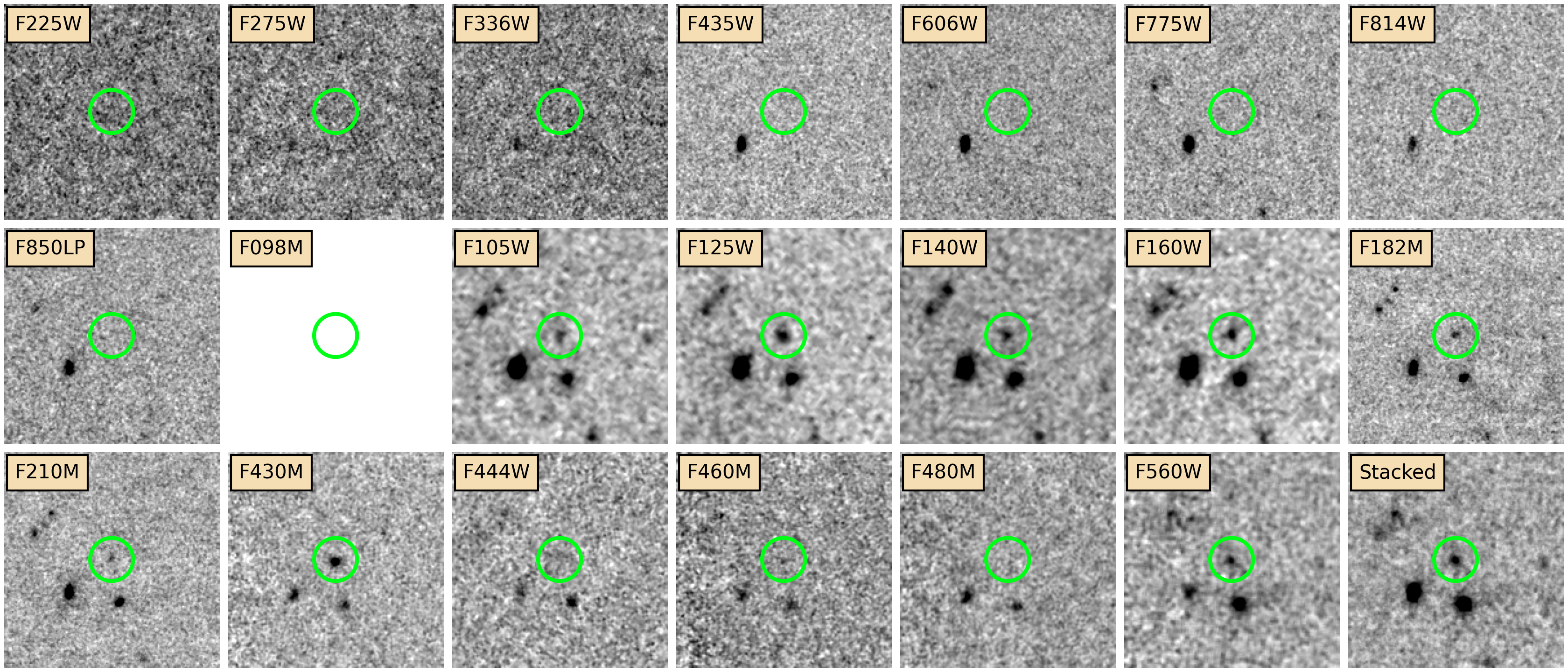
Figure 2: Postage stamps (5” $\times$ 5”) of one of our (H$\beta$ + [O III]) candidates (ID: 9434, z_best = 7.68 ${}_{-0.01}^{+0.03}$). The last postage stamp refers to the stacked image we adopted as the detection map with SExtractor. Here we show all the bands we used in our analysis, from 0.2$\mu$m to 5.6$\mu$m. The green circle has been placed to only guide the eye on the source. In particular, from these postage stamps, there is a clear excess at 4.3$\mu$m. This source shows an excess in MIRI/F560W as well.

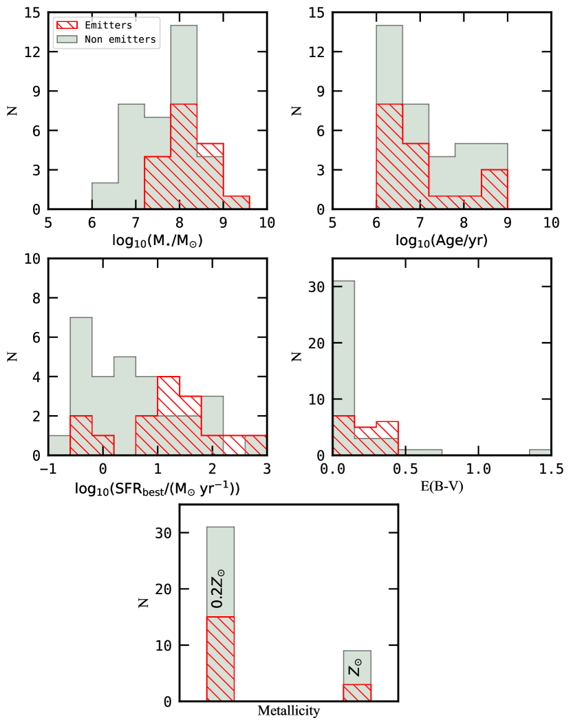
Figure 3: Comparison of the best-fit properties for emitters ((H$\beta$ + [O III]) and H$\alpha$) and non-emitters at $z=7-8$: stellar mass and age (upper row); star formation rate and colour excess (middle row); and metallicity (bottom row). No significant differences have been noticed between the two populations for most of the stellar parameters, as determined by performing a two-sample Kolmogorov-Smirnov test. Differences in SFR_best between emitters and non-emitters might be explained by the fact we are only looking at strong emitters that show a higher SFR_best.

4 Results

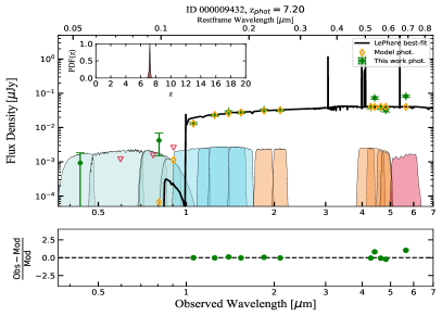
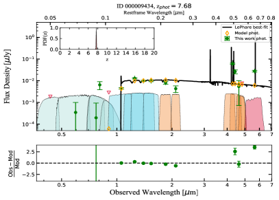
Figure 4: The best-fit SEDs for two examples of line-emitter candidates at $z\simeq 7-8$. On the left panel, we show a source at $z_{phot}\simeq 7.19$ (ID = 9432). On the right panel, we show another source at $z_{phot}\simeq 7.68$ (ID = 9434, shown in Fig. 2). Both panels show how well-constrained the best-fit SEDs and the derived photometric redshifts are, which is evident by simple inspection of the best-fit templates and their probability density functions (PDF(z)). In each case, we notice the clear presence of an excess in F430M, F444W, and F560W, which we adopted as the criterion to select our sample of (H$\beta$ + [O III]) and H$\alpha$ emitters.

Once we estimated the stellar properties of our candidates by performing the SED fitting with LePHARE, we analysed the properties of these sources by comparing our results with the recent literature at high redshifts. Before doing that, we first ensured that the stellar masses we inferred with LePHARE were not affected by the presence of the flux excess we estimated in F430M, F444W, and F560W. To do that, we re-run LePHARE following the methodology explained by Caputi et al. (2017). This time, for each source, we turned off those bands (NIRCam/F430M, NIRCam/F444W, and MIRI/F560W) in which we found a flux excess (i.e., $-99$ following LePHARE’s prescription). Moreover, for this run, we fixed the redshifts adopting the photometric ones we estimated from the original run. Doing this test allows us to ensure that our stellar mass estimates are not affected by any emission line that falls in one of those filters. We found a good agreement within 2$\sigma$. Finally, we also inspected that the stellar continuum was well-described by inspecting the best-fit SEDs we obtained from LePHARE. In Fig. 4 we show two examples (ID: 9432, 9434) of the best-fit SEDs for the candidates we have in our sample.

4.1 Emission line EW versus Stellar Mass and Age in galaxies at z $\simeq 7-8$

Having calculated the (H$\beta$ + [O III]) EW₀ for the prominent line emitters, we can compare their best-fit SED properties with those of the other $z\simeq 7-8$ galaxies in our sample. In Fig. 5, we show the derived (H$\beta$ + [O III]) EW₀ versus best-fit age. From this plot, we can see that all except three of the (H$\beta$ + [O III]) emitters are characterised by young best-fit ages ($\leq 10^{8}\,\rm yr$), which indicates that these objects may be in their first major star-formation episode. The remaining three objects are older ($>10^{8}\,\rm yr$), with two having almost the age of the Universe at their redshifts. This fact suggests that these galaxies could be having a rejuvenation episode, as is known to happen at lower redshifts (Rosani et al., 2020), as it is unlikely that they could have sustained their high instantaneous SFR values for all of their lifetimes.

The grey triangles in Fig. 5 refer to the EW upper limits that we estimated for all those galaxies at $z\simeq 7-8$ that do not have a significant flux excess in the NIRCam/F430M band. In contrast to the (H$\beta$ + [O III]) emitters, the non-emitters span different possible ages at those redshifts, without any bias towards young/old ages.

We also compared our results with the recent literature. In particular, Endsley et al. (2021) studied a sample of 20 rest-frame ultraviolet (UV) bright (H${\beta}$ + [O III]) emitters at $z\simeq 6.8-7$ that have been selected over a wide sky area (2.7 deg² in total). Endsley et al. (2021) found this rare population of very strong (H${\beta}$ + [O III]) emitters with an EW₀ $>1200$ Å. The fact that we find similarly high (H${\beta}$ + [O III]) EWs₀ among faint galaxies in a much smaller area of the sky indicates that prominent (H${\beta}$ + [O III]) emitters were much more common at the EoR than what can be inferred from the brightest galaxies.

Finally, the solid and dashed lines in Fig. 5 show the expected variation of the H$\beta$ (only) EW₀ versus age for SB99 model galaxies. These theoretical tracks are based on a Chabrier IMF with a stellar mass cut-off of $100M_{\odot}$ and were obtained both for a solar and a subsolar metallicity ($0.2Z_{\odot}$), each for a single burst and constant SFH. As expected, our data points are located nicely above these curves, following the trend of the models with constant star formation histories, albeit with higher EW₀, due to the [O III] contribution.

Over the past decades, the recombination line equivalent widths have been used as proxies for stellar population age in star-forming galaxies. The ratios between the fluxes of the recombination line, which are sensitive to the instantaneous star-formation rates, and the fluxes of the continuum, which are sensitive to the previous average SFR, are indeed what we define as recombination line equivalent widths (Stasińska & Leitherer, 1996). In particular, Reddy et al. (2018) found a very strong anti-correlation between (H$\beta$ + [O III]) EW₀ and young ages at $z\simeq 1.8-3.8$, which does not evolve as a function of redshift at that range of cosmic time. By looking at Fig. 5, we can see that this anti-correlation is evident also at $z\simeq 7-8$ where strong (H${\beta}$ + [O III]) emitters prefer young ages, which is in line with what has been found at lower redshifts. We double-checked this result by estimating the Spearman’s rank correlation coefficient, finding that those two quantities anti-correlate (i.e., Spearman’s coefficient $\simeq$ $-$0.5) with a p-value $\simeq$ 0.03. Therefore, we can conclude that there is evidence of a moderate anti-correlation between age and $\mathrm{EW_{0}}$(H$\beta$ + [O III]).

We repeated the same exercise looking, this time, at the derived (H$\beta$ + [O III]) EW₀ versus stellar mass for our (H$\beta$ + [O III]) emitters (Fig. 6). Also, in this case, the stellar masses come directly from the best-fit SED obtained with LePHARE. As we can see from Fig. 6, our (H$\beta$ + [O III]) emitters have a stellar mass that ranges from a minimum value of log₁₀(M_⋆/M_⊙) $\simeq$ 7.5 to a maximum value of log₁₀(M_⋆/M_⊙) $\simeq$ 9. In previous works, it has been shown that the normalization of the (H$\beta$ + [O III]) EW₀ versus stellar mass relation should increase with redshift (e.g., Reddy et al., 2018). Here we find a broad anti-correlation between the two quantities. The grey triangles in Fig. 6 refer to the upper limits that we estimated for the (H$\beta$ + [O III]) EW₀ for the $z\simeq 7-8$ galaxies that are not classified as emitters from a NIRCam flux excess.

Finally, for all those galaxies that show an “H$\alpha$ excess”, we compare their (H$\beta$ + [O III]) EW₀ versus H$\alpha$ EW₀, where the “H$\alpha$ excess” has been corrected to only take into account the real H$\alpha$ flux following Anders & Fritze-v. Alvensleben (2003). We show this comparison in Fig. 7. In particular, we also plot the recent results from Prieto-Lyon et al. (2022) where they inferred those quantities studying a sample of galaxies at $z\approx 3-7$. We see that our sample is in good agreement with the expected correlation that has been found in Prieto-Lyon et al. (2022) as well. As a matter of fact, as we can derive the H$\alpha$ line flux from our data, we can also infer the H$\beta$ line flux independently and separate the contributions of H$\beta$ and [O III] for each galaxy, considering the following:

$$f(H\beta)=f(H\alpha)\times 10^{-0.4\times 1.27E(B-V)}/2.86,$$ (2)

where $f(\rm H\alpha)$ and $f(\rm H\beta)$ refer to the observed fluxes and $E(B-V)$ is the colour excess obtained from the best-fit SED model. The denominator 2.86 corresponds to assuming case B recombination (e.g. Osterbrock & Ferland, 2006), while the factor $-1.27=k(\rm H\alpha)-k(\rm H\beta)$ is obtained from the Calzetti et al. (2000) reddening law.

Once we know the H$\beta$ flux for each source, we can independently work out the [O III]$\lambda\lambda$4959, 5007 fluxes for all those emitters that show an H$\alpha$ excess.

The data points in Fig. 7 are colour-coded according to each galaxy’s [O III]$\lambda$5007/H$\beta$ ratio. From that figure, we see that most line emitters have [O III]/H$\beta>1$, indicating the predominance of [O III], which is consistent with recent literature findings at similar redshifts. Instead, two galaxies have [O III]/H$\beta<1$, i.e. the H$\beta$ line flux is larger than the [O III] line flux for them. These two galaxies are well above the identity line in Fig. 7, as expected. We separate the H$\beta$ and [O III]$\lambda$5007 line fluxes simply assuming the case-B recombination H$\alpha$/H$\beta$=2.86 ratio and the corresponding colour excess mentioned above. The [O III]/H$\beta<1$ values could indicate very low metallicities, but this would need to be confirmed with a spectroscopy follow-up of these sources.

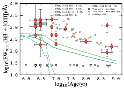
Figure 5: Age versus (H$\beta$ + [O III]) EW₀ for our line emitters at $z=7-8$. The grey triangles refer to the EW₀ upper limits that we estimated for all the “non-emitter” galaxies in our sample. We also show the data points from Endsley et al. (2021) to make a comparison with the recent literature at high redshift, albeit in a much higher luminosity regime. The curves refer to the evolution of the H$\beta$ EW₀ as a function of age expected from SB99 models, corresponding to the two metallicities (solar and sub-solar) that we have considered in our work and for two different SFHs. A clear anti-correlation between EW₀ and age is evident in this plot, which is in line with previous findings in the literature at lower redshifts (Reddy et al., 2018).

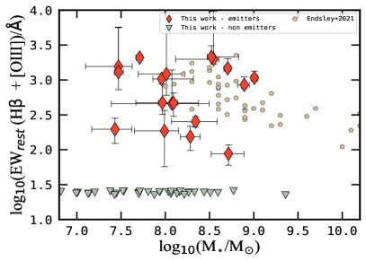
Figure 6: Stellar mass versus (H$\beta$ + [O III]) EW₀. The grey triangles refer to the upper limits we estimated for all those galaxies we classified as “non-emitters” during our selection. Also in this case, we report data points from Endsley et al. (2021) to make a comparison with the recent literature at high redshift. The EW₀ broadly anti-correlates with stellar mass, similarly to what has been reported by Reddy et al. (2018) and Endsley et al. (2021) at lower redshifts.

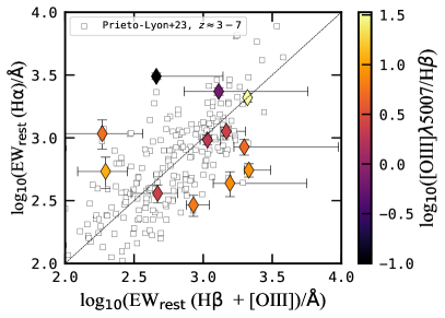
Figure 7: (H$\beta$ + [O III]) EW₀ versus H$\alpha$ EW₀. Here we colour-coded our data points for the [O III]$\lambda$5007/H$\beta$ flux ratio. Most galaxies have [O III]$\lambda$5007/H$\beta$ $>$ 1 and they mostly lie on or below the identity line. Among the four galaxies that lie above the identity line, two have [O III]$\lambda$5007/H$\beta$ $<$ 1, i.e., these line ratios are dominated by H$\beta$. Instead, the other two galaxies above the identity line have [O III]$\lambda$5007/H$\beta$ $>$ 1 and correspond to cases with non-negligible dust extinction.

4.2 H$\alpha$-derived SFR and the location of galaxies on the SFR-M_⋆ plane

For all the 12 H$\alpha$ emitters at $z\simeq 7-8$ as determined from the MIRI $5.6\,\rm\mu m$ imaging, we estimated their star formation rate (SFR) from their inferred H$\alpha$ luminosities.

After we obtained the net observed H$\alpha$ flux for each source, we converted those fluxes into the intrinsic ones by simply applying the Calzetti reddening law. We then estimate the luminosity for the H$\alpha$ emission line and apply the following formula from Kennicutt (1998) to obtain the corresponding SFR(H$\alpha$):

$$\mathrm{SFR(M_{\odot}\;yr^{-1})}=7.9\times 10^{-42}\;\mathrm{L_{H\alpha}}\mathrm{(erg}\;\mathrm{s^{-1}).}$$ (3)

Since the aforementioned formula has been originally calibrated for a Salpeter IMF over $\rm(0.1-100)\;M_{\odot}$ (Salpeter, 1955), we applied a conversion factor (Madau & Dickinson, 2014, i.e. 1.55) to rescale it to a Chabrier IMF (Chabrier, 2003).

We then placed our sources on the SFR$-$M_⋆ plane, as we show in Fig. 8. To make a comparison with the recent literature, we also populated this plane with star-forming galaxies at $z\simeq 3.0-6.5$ from Rinaldi et al. (2022) and (H$\beta$+[O III]) emitters at $z\simeq 6.8-7$ (Endsley et al., 2021). We also indicate the starburst (SB) zone as determined in Caputi et al. (2017, 2021), which empirically defined as starburst galaxies all those sources with a specific SFR (sSFR) $\mathrm{>10^{-7.60}\;yr^{-1}}$.

We see that 5 ($\simeq 42$%) of the galaxies that show an “H$\alpha$ excess” lie in the starburst zone, while only two are located on the star-formation main sequence (MS; Brinchmann et al., 2004; Noeske et al., 2007; Peng et al., 2010; Speagle et al., 2014; Rinaldi et al., 2022). The remaining 5 galaxies appear close, but slightly below the starburst envelope, in what has been defined in Caputi et al. (2017) as the star formation valley (SFV), i.e. in between the starburst cloud and the MS, suggesting that they are on the way to/from a starbursting phase. The fact that the vast majority of emitters are in or close to the starburst zone is consistent with the findings of Endsley et al. (2021) for brighter galaxies, as it can be seen in Fig. 8.

We also colour-coded our H$\alpha$ emitters according to their [O III]$\lambda 5007$/H$\beta$ ratios. We find no correlation between these ratios and the position of galaxies on the SFR$-$M_⋆ plane.

For the H$\alpha$ sample in Fig. 9a we show the comparison between the two different SFR indicators that we considered in this paper (UV and H$\alpha$ luminosities). From that plot, we clearly see differences between those two indicators ($\mathrm{SFR_{H\alpha}}$ and $\mathrm{SFR_{UV}}$). This finding is not surprising as it has been already pointed out in the literature (e.g., Flores Velázquez et al., 2021; Atek et al., 2022; Patel et al., 2023).

Differences between these two SFR tracers (Fig. 9a) may be partly explained by uncertainties in the dust-extinction correction, which mostly affect the UV continuum fluxes, and by our assumption that the dust extinction of the continuum and emission lines is the same and only depends on wavelength. However, part of the scatter observed in the $\rm SFR_{H\alpha}$ and $\rm SFR_{UV}$ plane may be real and due to the following:

• In very young galaxies (below 100 Myr), $\mathrm{SFR_{UV}}$ underestimates the real value because the UV luminosity associated with star formation is still growing. Indeed, when comparing $\rm SFR_{H\alpha}$ and $\rm SFR_{UV}$, one has to take into account age effects as well. UV traces typically 1500-2000Å (i.e., non-ionizing photons), while H$\alpha$ traces directly $<$ 912Å photons. For example, UV-bright regions without H$\alpha$ emission trace the presence of star-forming clumps dominated by B-type stars and where most massive O-type have already evolved;

• Different ionizing photon production efficiencies (e.g., Nanayakkara et al., 2020; Endsley et al., 2022; Rinaldi et al., 2023, in prep.).

Finally, by exploiting the FIRE simulations (Hopkins et al., 2014), Sparre et al. (2017) showed that the H$\alpha$ measurement of the SFR over a short timescale can fluctuate significantly, up to a factor of ten, compared to the UV indicator.

Following Atek et al. (2022) procedure at lower redshifts, in Fig. 9b we inspected the ratio between SFR_Hα and SFR_UV as a function of the stellar mass. We find similar results as Atek et al. (2022, see their Fig. 8) where the ratio of SFR_Hα/SFR_UV seems to be generally higher for the low-mass galaxies. Similarly, Faisst et al. (2019) find that more than 50% of their sample has SFR_Hα in excess compared to SFR_UV, particularly in low-mass galaxies. However, there are still uncertainties in determining the ratio of SFR_Hα/SFR_UV and how it changes with different galaxy parameters. As we know from the literature, the SFR indicators use conversion factors from H$\alpha$ and UV luminosities, which assume that the star formation rate is constant. Nonetheless, this assumption may not be that accurate for different SFHs, especially when we consider cases of bursty star formation.

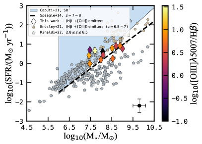
Figure 8: Stellar mass versus SFR. Here we show the SFR$-$M_⋆ plane populated by the SFR directly inferred from the “H$\alpha$ excess”. To make a comparison with the recent literature at high redshifts, we plot data points from Rinaldi et al. (2022) that give us the opportunity to populate this plane with very low-mass galaxies at $z\simeq 2.8-6.5$. We also show data points from Endsley et al. (2021), who studied a sample of 20 bright (H$\beta$ + [O III]) emitters at $z\simeq 6.8-7$, and indicate the starburst zone, as defined by Caputi et al. (2017, 2021). We also plot the expected main-sequence of galaxies at $z\simeq 7-8$ from Speagle et al. (2014). Our data points are colour-coded by their [O III]/H$\beta$ ratio. We see no correlation between this ratio and the position of sources on the SFR$-$M_⋆ plane.

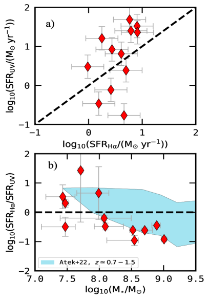
Figure 9: a) Comparison between $\mathrm{SFR_{UV}}$ and $\mathrm{SFR_{H_{\alpha}}}$. Error bars reflect the usual scatter that has been observed with the Kennicutt’s relations we used to derive those two quantities. b) The ratio of $\mathrm{SFR_{H_{\alpha}}}$ and $\mathrm{SFR_{UV}}$ as a function of stellar mass. Both SFRs have been corrected by adopting the same reddening curve (Calzetti et al., 2000). The horizontal line indicates a one-to-one ratio. The pale blue shade refers to Atek et al. (2022) results at lower redshifts.

4.3 The role of the H$\alpha$ emitters in the Cosmic Star Formation History at $z\simeq 7-8$

With the SFR values derived in the previous section, we computed the contribution of the prominent H$\alpha$ emitters to the cosmic Star Formation Rate Density (SFRD) at $z\simeq 7-8$. To do that, we sum up the individual SFRs ($\rm SFR_{H\alpha,total}\simeq 51.39\;M_{\odot}\;yr^{-1}$) and then divide the total by the comoving volume encompassed by the area ($\rm A\simeq 4.7\;arcmin^{2}$) and redshift bin (i.e., $z\simeq 7-8$) analysed in this work ($\rm V_{sky}\simeq 11580.26\;Mpc^{3}$). We obtain that, at these redshifts, the H$\alpha$ emitters make for $\mathrm{log_{10}(\rho_{SFR_{H\alpha}}/(M_{\odot}\;yr^{-1}\;Mpc^{-3}))\simeq-2.35\pm 0.3}$.

In Fig. 10 we show the redshift evolution of the SFRD as proposed by Lilly et al. (1996) and Madau et al. (1996), the so-called “Lilly-Madau diagram”. In this plot, we show our own estimation of the SFRD, along with a compilation of recent results from the literature based on different SFR tracers. In particular, we also show the SFRD values that have recently been obtained by Bouwens et al. (2022) using JWST data, tracing the SFR directly from the UV continuum emission at $z\simeq 9$ to $z\simeq 15$ as well as Pérez-González et al. (2023) results at $z\simeq 8-13$ from ultra-deep NIRCam images in HUDF-P2 (PID proposal: 1283, PI: Göran Östlin). Our inferred SFRD appears to be in good agreement with what has been found in the literature at similar redshifts. We also find a very good agreement with the predictions from theoretical models (e.g., IllustrisTNG; Springel et al., 2018). In particular, in Fig. 10 we also show the total SFRD, which has been estimated from both H$\alpha$ emitters and non-emitters at $z\simeq 7-8$ ($\mathrm{log_{10}(\rho_{SFR_{tot}}/(M_{\odot}\;yr^{-1}\;Mpc^{-3}))\simeq-1.76\pm 0.3}$). For the non-emitters, the SFR has been obtained from the rest-frame UV continuum luminosity at $2000\,\rm\AA$ and adopting the conversion formula from Kennicutt (1998).

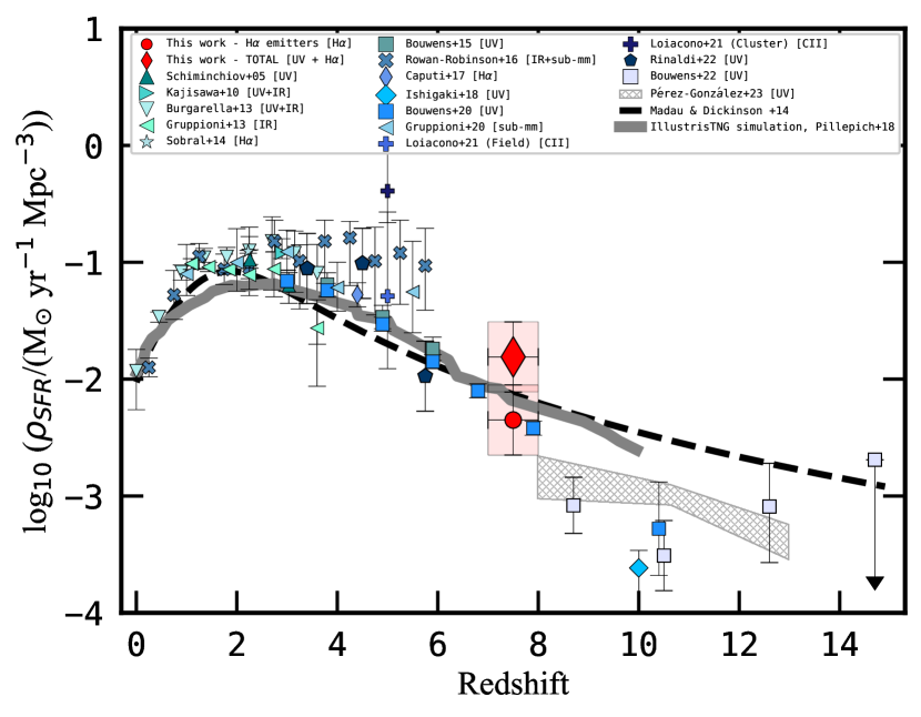
Figure 10: Cosmic star formation rate density as a function of the redshift. The large red circle at $\mathrm{log_{10}(\rho_{SFR_{H\alpha}}/(M_{\odot}\;yr^{-1}\;Mpc^{-3}))\simeq-2.35}$ indicates our estimate at $z\simeq 7-8$, which only takes into account the prominent H$\alpha$ emitters, i.e., it should be considered a lower limit to the real SFRD value at these redshifts. The red diamond at $\mathrm{log_{10}(\rho_{SFR_{tot}}/(M_{\odot}\;yr^{-1}\;Mpc^{-3}))\simeq-1.76}$, instead, refers to the total SFRD we estimated taking into account both the H$\alpha$ emitters and non-emitters at $z\simeq 7-8$. For the non-emitters, the SFR directly comes from the UV continuum emission. Other symbols refer to the recent SFRD determinations from the literature, based on different SFR tracers (Schiminovich et al., 2005; Kajisawa et al., 2010; Burgarella et al., 2013; Gruppioni et al., 2013; Sobral et al., 2014a; Bouwens et al., 2015; Rowan-Robinson et al., 2016; Caputi et al., 2017; Ishigaki et al., 2018; Bouwens et al., 2020; Gruppioni et al., 2020; Loiacono et al., 2021; Rinaldi et al., 2022; Bouwens et al., 2022; Pérez-González et al., 2023). The different curves correspond to theoretical predictions. Dashed line: Madau & Dickinson (2014). Solid line: Pillepich et al. (2018). All the SFRD values in this figure correspond to a Chabrier (2003) IMF.

4.4 The evolution of the rest-frame EW(H$\alpha$) as a function of redshift

Finally, our derived values of the H$\alpha$ EW₀ allow us to extend the study of the redshift evolution of this parameter to $z\simeq 7-8$. In Fig. 11 we present our results along with the most recent determinations from the literature (for sources at $z\simeq 0.5-6$, Erb et al., 2006; Shim et al., 2011; Fumagalli et al., 2012; Stark et al., 2013; Sobral et al., 2014b; Mármol-Queraltó et al., 2016; Smit et al., 2016; Reddy et al., 2018; Lam et al., 2019; Atek et al., 2022; Boyett et al., 2022; Sun et al., 2022; Ning et al., 2023) and a stacking analysis measurement by (Stefanon et al., 2022) at $z\simeq 8$. These previous works made use of different methods and techniques to determine the H$\alpha$ EW, such as medium/high-resolution spectroscopy, low-resolution grism spectroscopy, and narrow-band and broad-band photometry combined with SED modelling, as we did in this paper.

Our sample of strong line emitters at $z\simeq 7-8$ allows us to populate a virtually unexplored part of parameter space. At those redshifts ($z\simeq 8$), only Stefanon et al. (2022) previously obtained an estimate of the average H$\alpha$ EW₀, by median stacking 102 Lyman-break galaxies (LBG) in the 3.6$\mu$m, 4.5$\mu$m, 5.8$\mu$m, and 8.0$\mu$m bands from the Spitzer Infrared Array Camera (IRAC).

We also incorporate in the analysis the empirical prescriptions from Fumagalli et al. (2012) and Faisst et al. (2016), who predict that the EW₀(H$\alpha$) should evolve differently below and above $z\simeq 2$. Particularly, according to the recent literature, at $z<2$, the EW₀(H$\alpha$) should evolve as $\propto(1+z)^{1.8}$, while at $z>2$ it should evolve as $\propto(1+z)^{1.3}$.

By inspection of Fig. 11, we can see that JWST observations at $z\geq 6$ (i.e., Sun et al., 2022; Ning et al., 2023, and this present work) suggest that the break proposed at $z\simeq 2$ in the past literature does not really hold up to such high redshifts (tiny, black, and dashed line). For that reason, we fit the evolution of EW$\mathrm{{}_{0}(H\alpha)}$ as a function of redshift again by considering the recent JWST observations at $z\geq 6$ as well. In this case, we find that EW$\mathrm{{}_{0}(H\alpha)\propto(1+z)^{2.1}}$ (bold, dark red, and dashed line in Fig 11). However, larger galaxy samples are needed to confirm this finding.

Our data points are in good agreement with the stacking estimate obtained by Stefanon et al. (2022). Some of these values are well above the empirical median extrapolation at those redshifts, while others are consistent with it. The prominent line emitters we analyse here constitute almost a quarter of all the MIRI-detected galaxies at $z\simeq 7-8$. The remaining MIRI sources at those redshifts should lie below the extrapolation of the empirical determination. This very large variation in the H$\alpha$ EW₀ at $z\simeq 7-8$ suggests that, even at these very high redshifts, galaxies may be at different stages of their evolution, as we discuss in the next section.

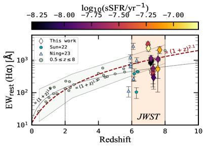
Figure 11: Evolution of the EW₀(H$\alpha$) as a function of redshift. After re-fitting all the data points, including our own, we find that the EW₀(H$\alpha$) evolution can be described by a single law: EW$\mathrm{{}_{0}(H\alpha)\propto(1+z)^{2.1}}$ (bold, dark red, and dashed line.) Our data points are colour-coded for sSFR. We also report the recent literature regarding the evolution of the EW₀(H$\alpha$) as a function of the redshift (tiny, black, and dashed line). The grey shade represents a median estimate of the error bars of the data points from the literature. The orange shade represents the redshift window where JWST is starting to detect these kinds of sources more systematically (e.g., Boyett et al., 2022; Sun et al., 2022; Ning et al., 2023). Note that the data point at $z\simeq 8$ from Stefanon et al. (2022) has been obtained by median stacking a sample of 102 Lyman-break galaxies in the Spitzer/IRAC bands from 3.6$\mu$m to 8$\mu$m.

5 Summary and Conclusions

In this paper, we have taken advantage of the publicly available medium and broad-band NIRCam imaging in the XDF, combined with the deepest MIRI 5.6$\mu$m imaging existing in the same field, to search for prominent (H$\beta$+[O III]) and H$\alpha$ emitters at $z\simeq 7-8$. This is the first time the H$\alpha$ emission line can be detected and its flux measured in individual galaxies at such high redshifts. This has been possible thanks to the unprecedented sensitivity of JWST observations, particularly those conducted with MIRI, for which the sensitivity gain is of more than an order of magnitude with respect to previous instruments operating at similar wavelengths (Iani et al., 2022).

We found 18 galaxies which are robust candidates to be prominent (H$\beta$+[O III]) emitters at $z\simeq 7-8$, as determined from their F430M and F444W flux excess. These 18 galaxies constitute $\simeq 31\%$ of all the galaxies that we find in the XDF in the same redshift range. Among them, 16 lie on the MIRI coverage area and 12 out of 16 have a clear flux excess in the MIRI/F560W filter, indicating the simultaneous presence of a prominent H$\alpha$ emission line. The (H$\beta$+[O III]) EWs₀ that we derive range from $\simeq 87.5^{+30}_{-27}\,\rm\AA$ to $2140.4^{+970}_{-154}\,\rm\AA$, with a median value of $943_{-194}^{+737}\,\rm\AA$. For most of these galaxies, we find [O III]/H$\beta>1$, but a few have [O III]/H$\beta<1$. The two line fluxes can be separated by making use of the independent H$\alpha$ emission line measurement. This is telling us that some of the prominent (H$\beta$+[O III]) emitters likely have hard radiation fields typical of low-metallicity galaxies, but not all of them. Some are strong line emitters simply because they are intensively forming stars.

The identified H$\alpha$ emitters show an EW₀ that ranges from a few hundred to a few thousand Angstroms. Some of these values are substantially above the expected median H$\alpha$ EW at these redshifts, as extrapolated from lower redshift determinations. We also report that, by considering the recent JWST findings at $z\geq 6$ (including this present work), $\rm EW_{0}(H\alpha)$ as a function of the redshift should evolve as follows: $\rm EW_{0}(H\alpha)\propto(1+z)^{2.1}$. However, larger samples of galaxies are needed to confirm this result. We note, however, that the prominent H$\alpha$ emitters only constitute about a quarter of all the MIRI-detected galaxies at $z\simeq 7-8$. For the remaining galaxies, the H$\alpha$ EW₀ should lie below the expected median trend. As the H$\alpha$ EW is a good proxy for the sSFR, the lower EW values could indicate that these other galaxies (the non-emitters) have either relatively low star-formation rates, or a more important underlying stellar population producing a higher continuum. This is likely the case for the non-emitters at $z\simeq 7-8$ which are relatively evolved galaxies, with best-fit ages $>10^{7}-10^{8}$ yr and stellar masses $>10^{8}\,\rm M_{\odot}$.

In turn, most of the prominent (H$\beta$+[O III]) and H$\alpha$ emitters are characterised by higher sSFR, with basically all of them being starburst galaxies or on the way to/from the starburst cloud. The majority of the prominent (H$\beta$+[O III]) emitters are very young galaxies (best-fit ages $<10^{7}\,\rm yr$), so they might be in their first major star-formation episode. A few others are almost as old as the Universe at their redshifts and have already built significant stellar mass ($>10^{8}\,\rm M_{\odot}$), suggesting that they may be experiencing a rejuvenation effect.

Therefore, the overall conclusion of this work is that the galaxies present at the EoR are likely at different stages of their evolution. And strong line emission is present in a minor, but significant fraction of sources.

Considering the H$\alpha$ fluxes inferred for the prominent H$\alpha$ emitters, we estimated their contribution to the cosmic SFRD at $z\simeq 7-8$. We found $\mathrm{log_{10}(\rho_{SFR_{H\alpha}}/(M_{\odot}\;yr^{-1}\;Mpc^{-3}))\simeq-2.35\pm 0.3}$, in excellent agreement with independent measurements from the literature based on rest-frame UV luminosities, and with theoretical predictions and empirical extrapolations from lower redshifts. We note, however, that this estimated SFRD must be considered a lower limit, as it only takes into account the most prominent H$\alpha$ emitters at $z\simeq 7-8$. We also considered the SFR_UV for all the other galaxies at $z\simeq 7-8$ to obtain a total SFRD value at that redshift interval. We concluded that the strong H$\alpha$ emitters produced about a quarter of the total SFRD at $z\simeq 7-8$, which suggests that they likely have had a significant role in the process of reionization. In a future paper, we will conduct a more detailed investigation of these sources, in order to better understand their nature.

References

- Anders & Fritze-v. Alvensleben (2003) Anders, P., & Fritze-v. Alvensleben, U. 2003, A&A, 401, 1063
- Arellano-Córdova et al. (2022) Arellano-Córdova, K. Z., Berg, D. A., Chisholm, J., et al. 2022, ApJ, 940, L23
- Arnouts & Ilbert (2011) Arnouts, S., & Ilbert, O. 2011, LePHARE: Photometric Analysis for Redshift Estimate, , , ascl:1108.009
- Astropy Collaboration et al. (2018) Astropy Collaboration, Price-Whelan, A. M., Sipőcz, B. M., et al. 2018, AJ, 156, 123
- Atek et al. (2022) Atek, H., Furtak, L., Oesch, P., et al. 2022, arXiv e-prints, arXiv:2202.04081
- Babusiaux et al. (2022) Babusiaux, C., Fabricius, C., Khanna, S., et al. 2022, arXiv e-prints, arXiv:2206.05989
- Bagley et al. (2022) Bagley, M. B., Finkelstein, S. L., Koekemoer, A. M., et al. 2022, arXiv e-prints, arXiv:2211.02495
- Bertin & Arnouts (1996) Bertin, E., & Arnouts, S. 1996, A&AS, 117, 393
- Bouwens et al. (2020) Bouwens, R., González-López, J., Aravena, M., et al. 2020, ApJ, 902, 112
- Bouwens et al. (2015) Bouwens, R. J., Illingworth, G. D., Oesch, P. A., et al. 2015, ApJ, 803, 34
- Bouwens et al. (2022) Bouwens, R. J., Stefanon, M., Brammer, G., et al. 2022, arXiv e-prints, arXiv:2211.02607
- Boyett et al. (2022) Boyett, K., Mascia, S., Pentericci, L., et al. 2022, ApJ, 940, L52
- Bradley et al. (2021) Bradley, L., Sipőcz, B., Robitaille, T., et al. 2021, astropy/photutils: 1.0.2, v1.0.2, Zenodo, doi:10.5281/zenodo.4453725
- Brinchmann et al. (2004) Brinchmann, J., Charlot, S., White, S. D. M., et al. 2004, MNRAS, 351, 1151
- Bruzual & Charlot (2003) Bruzual, G., & Charlot, S. 2003, MNRAS, 344, 1000
- Burgarella et al. (2013) Burgarella, D., Buat, V., Gruppioni, C., et al. 2013, A&A, 554, A70
- Calzetti et al. (2000) Calzetti, D., Armus, L., Bohlin, R. C., et al. 2000, ApJ, 533, 682
- Caputi et al. (2011) Caputi, K. I., Cirasuolo, M., Dunlop, J. S., et al. 2011, MNRAS, 413, 162
- Caputi et al. (2017) Caputi, K. I., Deshmukh, S., Ashby, M. L. N., et al. 2017, ApJ, 849, 45
- Caputi et al. (2021) Caputi, K. I., Caminha, G. B., Fujimoto, S., et al. 2021, ApJ, 908, 146
- Caruana et al. (2014) Caruana, J., Bunker, A. J., Wilkins, S. M., et al. 2014, MNRAS, 443, 2831
- Chabrier (2003) Chabrier, G. 2003, PASP, 115, 763
- Coe (2015) Coe, D. 2015, Trilogy: FITS image conversion software, Astrophysics Source Code Library, record ascl:1508.009, , , ascl:1508.009
- De Barros et al. (2019) De Barros, S., Oesch, P. A., Labbé, I., et al. 2019, MNRAS, 489, 2355
- Endsley et al. (2021) Endsley, R., Stark, D. P., Chevallard, J., & Charlot, S. 2021, MNRAS, 500, 5229
- Endsley et al. (2022) Endsley, R., Stark, D. P., Whitler, L., et al. 2022, arXiv e-prints, arXiv:2208.14999
- Erb et al. (2006) Erb, D. K., Steidel, C. C., Shapley, A. E., et al. 2006, ApJ, 647, 128
- Faisst et al. (2019) Faisst, A. L., Capak, P. L., Emami, N., Tacchella, S., & Larson, K. L. 2019, ApJ, 884, 133
- Faisst et al. (2016) Faisst, A. L., Capak, P., Hsieh, B. C., et al. 2016, ApJ, 821, 122
- Flores Velázquez et al. (2021) Flores Velázquez, J. A., Gurvich, A. B., Faucher-Giguère, C.-A., et al. 2021, MNRAS, 501, 4812
- Fontana et al. (2010) Fontana, A., Vanzella, E., Pentericci, L., et al. 2010, ApJ, 725, L205
- Fumagalli et al. (2012) Fumagalli, M., Patel, S. G., Franx, M., et al. 2012, ApJ, 757, L22
- Galametz et al. (2013) Galametz, A., Grazian, A., Fontana, A., et al. 2013, ApJS, 206, 10
- Gruppioni et al. (2013) Gruppioni, C., Pozzi, F., Rodighiero, G., et al. 2013, MNRAS, 436, 2875
- Gruppioni et al. (2020) Gruppioni, C., Béthermin, M., Loiacono, F., et al. 2020, A&A, 643, A8
- Harris et al. (2020) Harris, C. R., Millman, K. J., van der Walt, S. J., et al. 2020, Nature, 585, 357. https://doi.org/10.1038/s41586-020-2649-2
- Hopkins et al. (2014) Hopkins, P. F., Kereš, D., Oñorbe, J., et al. 2014, MNRAS, 445, 581
- Iani et al. (2022) Iani, E., Caputi, K. I., Rinaldi, P., & Kokorev, V. I. 2022, ApJ, 940, L24
- Illingworth et al. (2013) Illingworth, G. D., Magee, D., Oesch, P. A., et al. 2013, ApJS, 209, 6
- Ishigaki et al. (2018) Ishigaki, M., Kawamata, R., Ouchi, M., et al. 2018, ApJ, 854, 73
- Kajisawa et al. (2010) Kajisawa, M., Ichikawa, T., Yamada, T., et al. 2010, ApJ, 723, 129
- Kennicutt (1998) Kennicutt, Robert C., J. 1998, ARA&A, 36, 189
- Khostovan et al. (2016) Khostovan, A. A., Sobral, D., Mobasher, B., et al. 2016, MNRAS, 463, 2363
- Kron (1980) Kron, R. G. 1980, ApJS, 43, 305
- Labbé et al. (2013) Labbé, I., Oesch, P. A., Bouwens, R. J., et al. 2013, ApJ, 777, L19
- Lam et al. (2019) Lam, D., Bouwens, R. J., Labbé, I., et al. 2019, A&A, 627, A164
- Langeroodi et al. (2022) Langeroodi, D., Hjorth, J., Chen, W., et al. 2022, arXiv e-prints, arXiv:2212.02491
- Leitherer et al. (2002) Leitherer, C., Li, I. H., Calzetti, D., & Heckman, T. M. 2002, ApJS, 140, 303
- Leitherer et al. (1999) Leitherer, C., Schaerer, D., Goldader, J. D., et al. 1999, ApJS, 123, 3
- Lilly et al. (1996) Lilly, S. J., Le Fevre, O., Hammer, F., & Crampton, D. 1996, ApJ, 460, L1
- Loiacono et al. (2021) Loiacono, F., Decarli, R., Gruppioni, C., et al. 2021, A&A, 646, A76
- Madau & Dickinson (2014) Madau, P., & Dickinson, M. 2014, ARA&A, 52, 415
- Madau et al. (1996) Madau, P., Ferguson, H. C., Dickinson, M. E., et al. 1996, MNRAS, 283, 1388
- Mármol-Queraltó et al. (2016) Mármol-Queraltó, E., McLure, R. J., Cullen, F., et al. 2016, MNRAS, 460, 3587
- Matthee et al. (2022) Matthee, J., Mackenzie, R., Simcoe, R. A., et al. 2022, arXiv e-prints, arXiv:2211.08255
- Morishita & Stiavelli (2022) Morishita, T., & Stiavelli, M. 2022, arXiv e-prints, arXiv:2207.11671
- Nanayakkara et al. (2020) Nanayakkara, T., Brinchmann, J., Glazebrook, K., et al. 2020, ApJ, 889, 180
- Ning et al. (2023) Ning, Y., Cai, Z., Jiang, L., et al. 2023, ApJ, 944, L1
- Noeske et al. (2007) Noeske, K. G., Weiner, B. J., Faber, S. M., et al. 2007, ApJ, 660, L43
- Oesch et al. (2021) Oesch, P., Bouwens, R., Brammer, G., et al. 2021, FRESCO: The First Reionization Epoch Spectroscopic COmplete Survey, JWST Proposal. Cycle 1, ID. #1895, ,
- Oesch et al. (2023) Oesch, P. A., Brammer, G., Naidu, R. P., et al. 2023, arXiv e-prints, arXiv:2304.02026
- Oke & Gunn (1983) Oke, J. B., & Gunn, J. E. 1983, ApJ, 266, 713
- Ono et al. (2012) Ono, Y., Ouchi, M., Mobasher, B., et al. 2012, ApJ, 744, 83
- Osterbrock & Ferland (2006) Osterbrock, D. E., & Ferland, G. J. 2006, Astrophysics of gaseous nebulae and active galactic nuclei
- Östlin et al. (2023, in prep.) Östlin, G., Colina, L., Caputi, K., & Collaborators. 2023, in prep.
- pandas development team (2020) pandas development team, T. 2020, pandas-dev/pandas: Pandas, vlatest, Zenodo, doi:10.5281/zenodo.3509134. https://doi.org/10.5281/zenodo.3509134
- Patel et al. (2023) Patel, S. G., Kelson, D. D., Abramson, L. E., Sattari, Z., & Lorenz, B. 2023, ApJ, 945, 93
- Peng et al. (2010) Peng, Y.-j., Lilly, S. J., Kovač, K., et al. 2010, ApJ, 721, 193
- Pentericci et al. (2014) Pentericci, L., Vanzella, E., Fontana, A., et al. 2014, ApJ, 793, 113
- Pérez-González et al. (2023) Pérez-González, P. G., Costantin, L., Langeroodi, D., et al. 2023, arXiv e-prints, arXiv:2302.02429
- Pillepich et al. (2018) Pillepich, A., Springel, V., Nelson, D., et al. 2018, MNRAS, 473, 4077
- Prieto-Lyon et al. (2022) Prieto-Lyon, G., Strait, V., Mason, C. A., et al. 2022, arXiv e-prints, arXiv:2211.12548
- Reddy et al. (2018) Reddy, N. A., Shapley, A. E., Sanders, R. L., et al. 2018, ApJ, 869, 92
- Rieke et al. (2015) Rieke, G. H., Wright, G. S., Böker, T., et al. 2015, PASP, 127, 584
- Rieke et al. (2005) Rieke, M. J., Kelly, D., & Horner, S. 2005, in Society of Photo-Optical Instrumentation Engineers (SPIE) Conference Series, Vol. 5904, Cryogenic Optical Systems and Instruments XI, ed. J. B. Heaney & L. G. Burriesci, 1–8
- Rinaldi et al. (2023, in prep.) Rinaldi, P., Caputi, K., & Collaborators. 2023, in prep.
- Rinaldi et al. (2022) Rinaldi, P., Caputi, K. I., van Mierlo, S. E., et al. 2022, ApJ, 930, 128
- Roberts-Borsani et al. (2016) Roberts-Borsani, G. W., Bouwens, R. J., Oesch, P. A., et al. 2016, ApJ, 823, 143
- Rosani et al. (2020) Rosani, G., Caminha, G. B., Caputi, K. I., & Deshmukh, S. 2020, A&A, 633, A159
- Rowan-Robinson et al. (2016) Rowan-Robinson, M., Oliver, S., Wang, L., et al. 2016, MNRAS, 461, 1100
- Salpeter (1955) Salpeter, E. E. 1955, ApJ, 121, 161
- Schaerer & de Barros (2009) Schaerer, D., & de Barros, S. 2009, A&A, 502, 423
- Schiminovich et al. (2005) Schiminovich, D., Ilbert, O., Arnouts, S., et al. 2005, ApJ, 619, L47
- Schlafly & Finkbeiner (2011) Schlafly, E. F., & Finkbeiner, D. P. 2011, ApJ, 737, 103
- Shim et al. (2011) Shim, H., Chary, R.-R., Dickinson, M., et al. 2011, ApJ, 738, 69
- Smit et al. (2016) Smit, R., Bouwens, R. J., Labbé, I., et al. 2016, ApJ, 833, 254
- Sobral et al. (2014a) Sobral, D., Best, P. N., Smail, I., et al. 2014a, MNRAS, 437, 3516
- Sobral et al. (2014b) —. 2014b, MNRAS, 437, 3516
- Sonnett et al. (2013) Sonnett, S., Meech, K., Jedicke, R., et al. 2013, PASP, 125, 456
- Sparre et al. (2017) Sparre, M., Hayward, C. C., Feldmann, R., et al. 2017, MNRAS, 466, 88
- Speagle et al. (2014) Speagle, J. S., Steinhardt, C. L., Capak, P. L., & Silverman, J. D. 2014, ApJS, 214, 15
- Springel et al. (2018) Springel, V., Pakmor, R., Pillepich, A., et al. 2018, MNRAS, 475, 676
- Stark et al. (2013) Stark, D. P., Schenker, M. A., Ellis, R., et al. 2013, ApJ, 763, 129
- Stark et al. (2015) Stark, D. P., Richard, J., Charlot, S., et al. 2015, MNRAS, 450, 1846
- Stasińska & Leitherer (1996) Stasińska, G., & Leitherer, C. 1996, ApJS, 107, 661
- Stefanon et al. (2022) Stefanon, M., Bouwens, R. J., Illingworth, G. D., et al. 2022, ApJ, 935, 94
- Sun et al. (2022) Sun, F., Egami, E., Pirzkal, N., et al. 2022, arXiv e-prints, arXiv:2209.03374
- Tang et al. (2019) Tang, M., Stark, D. P., Chevallard, J., & Charlot, S. 2019, MNRAS, 489, 2572
- Taylor (2005) Taylor, M. B. 2005, in Astronomical Society of the Pacific Conference Series, Vol. 347, Astronomical Data Analysis Software and Systems XIV, ed. P. Shopbell, M. Britton, & R. Ebert, 29
- Trump et al. (2022) Trump, J. R., Arrabal Haro, P., Simons, R. C., et al. 2022, arXiv e-prints, arXiv:2207.12388
- Virtanen et al. (2020) Virtanen, P., Gommers, R., Oliphant, T. E., et al. 2020, Nature Methods, 17, 261
- Wang et al. (2022) Wang, X., Cheng, C., Ge, J., et al. 2022, arXiv e-prints, arXiv:2212.04476
- Whitaker et al. (2019) Whitaker, K. E., Ashas, M., Illingworth, G., et al. 2019, ApJS, 244, 16
- Williams et al. (2023) Williams, C. C., Tacchella, S., Maseda, M. V., et al. 2023, arXiv e-prints, arXiv:2301.09780
- Williams et al. (2022) Williams, H., Kelly, P. L., Chen, W., et al. 2022, arXiv e-prints, arXiv:2210.15699
- Wright et al. (2015) Wright, G. S., Wright, D., Goodson, G. B., et al. 2015, PASP, 127, 595