Polar magneto-optic Kerr and Faraday effects in finite periodic $\mathcal{P}\mathcal{T}$-symmetric systems

Abstract

We discuss the anomalous behavior of the Faraday (transmission) and polar Kerr (reflection) rotation angles of the propagating light, in finite periodic parity-time ($\mathcal{P}\mathcal{T}$) symmetric structures, consisting of $N$ cells. The unit cell potential is two complex $\delta$-potentials placed on both boundaries of the ordinary dielectric slab. It is shown that, for a given set of parameters describing the system, a phase transition-like anomalous behavior of Faraday and Kerr rotation angles in a parity-time symmetric systems can take place. In the anomalous phase the value of one of the Faraday and Kerr rotation angles can become negative, and both angles suffer from spectral singularities and give a strong enhancement near the singularities. We also shown that the real part of the complex angle of KR, $\theta^{R}_{1}$, is always equal to the $\theta^{T}_{1}$ of FR, no matter what phase the system is in due to the symmetry constraints. The imaginary part of KR angles $\theta^{R^{r/l}}_{2}$ are related to the $\theta^{T}_{2}$ of FR by parity-time symmetry. Calculations based on the approach of the generalized nonperturbative characteristic determinant, which is valid for a layered system with randomly distributed delta potentials, show that the Faraday and Kerr rotation spectrum in such structures has several resonant peaks. Some of them coincide with transmission peaks, providing simultaneous large Faraday and Kerr rotations enhanced by an order one or two of magnitude. We provide a recipe for funding a one-to-one relation in between KR and FR.

I Introduction

The study of the magneto-optic effects (Faraday rotation (FR) and Kerr rotation (KR)), has played an important role in the development both of electromagnetic theory and atomic physics. The magneto-optical materials that exhibiting FR and KR are essential for optical communication technology Yoshino (2005); Zamani et al. (2011); Birch (1982), optical amplifiers Corzo et al. (2012); Stubkjaer (2000), and photonic crystals Wang et al. (2008, 2009). In addition to this important application, the KR is also an extremely accurate and versatile research tool and can be used to determine quantities as varied as anisotropy constants, exchange-coupling strengths and Curie temperatures (see, e.g., McGee et al. (1993).)

In polar or magneto-optical Kerr effect, the magnetization of the system is in the plane of incidence and perpendicular to the reflecting surface. Reflection can produce several effects, including 1) rotation the direction of light polarization, 2) introducing ellipticity into the reflected beam, and 3) changing by the intensity of the reflected beam.

FR is similar to KR in terms of rotation and ellipticity and has a wide range of applications in various fields of modern physics, such as measuring magnetic field in astronomy Longair (2011) and construction of optical isolators for fiber-optic telecommunication systems Furdyna (1988), as well as the design of optical circulators used in the development of microwave integrated circuits. Berger (2003); Turner and Stolen (1981); Firby et al. (2018).

Note, that large Faraday and Kerr rotations are needed for all the applications mentioned. However, the standard method, based on increasing the sample size or applying a strong external magnetic field, is currently ineffective due to the small size of systems in which the de Broglie wavelength is compatible with the size of quantum devices. In other words, thin film materials exhibiting a large FR angle should be desirable for promote progress optical integrated circuits.

A large enhancement of the FR and as well as a change in the sign of the FR can be obtained by incorporating several nanoparticles and their composites in nanomaterials, see e.g. Refs. Uchida et al. (2011); Andrei and Mayergoyz (2003); Gevorkian and Gasparian (2014). A phase transition-like anomalous behavior of Faraday rotation angles in a simple parity-time $\mathcal{P}\mathcal{T}$-symmetric model of a regular dielectric slab was reported recently in Ref.Gasparian et al. (2022a). In anomalous phase, the value of one of Faraday rotation angles turns negative, and both angles suffer spectral singularities and yield strong enhancement near singularities.

As for the enhancing of the KR, in which we are interested too, it is mainly related to spin-orbit coupling strength Oppeneer et al. (1992), to interference effects Chen et al. (1990) and as well as by the plasma resonance of the free carriers of magnetic materials Feil and Haas (1987). As it was mentioned in Ref. Loughran et al. (2018), with addition of a gold nano-disc to the periodic magnetic system, yields a strong wavelength-dependent enhancement of the KR. Generally, the enhancement factor is expected to be less than three even for materials with high refractive index $\approx 2$, such as semiconductors with zero extinction coefficients in the near or mid infrared range (like tellurium or aluminum gallium arsenide).

In this paper we aim to present a complete and quantitative theoretical description of the Faraday and Kerr complex rotations for an arbitrary one dimensional finite periodic $\mathcal{P}\mathcal{T}$-symmetric system, consisting from (2N+1) cells for some simple cases we give simple closed form expressions, describing the FR and KR.

We illustrate that the Faraday and Kerr rotation angles of the polarized light traveling through a $\mathcal{P}\mathcal{T}$-symmetric periodic structure display phase transition-like anomalous behaviors.

In one phase (normal phase), the FR and KR angles behave normally as in regular passive system with a positive permittivity, and stay positive all the time as expected. In the second anomalous phase, the angle of FR and KR angles may change the sign and turn into negative. In addition, spectral singularities arise in the second anomalous phase, where the angles FR and KR increase strongly. In this sense, $\mathcal{P}\mathcal{T}$-systems seem to be a good candidate for constructing fast tunable and switchable polarization rotational ultrathin magneto-optical devices in a wide frequency range with a giant FR and KR rotations. Despite that the obtained results are, in general, only suitable for numerical analysis. However, in some simple cases approximate expressions can be derived and a qualitative discussion is possible.

The paper is organized as follows. In Sec. II the complex Faraday and Kerr effects are introduced and discussed for $\mathcal{P}\mathcal{T}$-symmetric unit cell with two complex $\delta$-potentials. We will assume that the strengths of two Dirac $\delta$ functions $Z_{1}$ and $Z_{2}$ are arbitrary complex numbers. The periodic system with $2N+1$ cells is is discussed in Sec. III. Followed by the discussions and summary in Sec. IV.

II General theory of Faraday and Kerr effects in $\mathcal{P}\mathcal{T}$-symmetric dielectric slabs

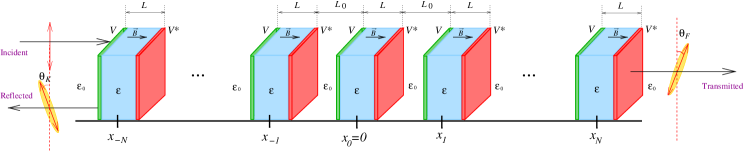
Figure 1: Schematic of a one-dimesnionl $\mathcal{P}\mathcal{T}$-symmetric photonic heterostructure, consisting of $2N+1$ arbitrary number of slabs that are $\mathcal{P}\mathcal{T}$ -symmetric about $x_{0}=0$, that is $\epsilon(x)=\epsilon^{*}(-x)$. Each slab of the photonic heterostructure, has two balanced complex tiny slabs placed at both ends of a real dielectric slab. The green slab indicates the loss and the red slab indicates the gain region.

In this section, before discussing in detail the Faraday and Kerr effects in a simple unit cell—an ordinary dielectric slab with two complex $\delta$-potentials located at both boundaries (the unit cell located symmetrically about $x_{0}=0$ in Fig. 1), we present some details of the rotation angle calculation for an arbitrary one-dimensional dielectric permittivity profile $\epsilon(x)$. Later, we will impose the condition $\epsilon(x)=\epsilon^{*}(-x)$, which guarantees the system is $\mathcal{P}\mathcal{T}$-symmetric, that its eigenstates are real-valued solutions. In such a $\mathcal{P}\mathcal{T}$-symmetric dielectric system with a finite spatial extension in $x$ direction (see Fig. 1), the permittivity of the system (as well as the single slab) has a balanced gain and loss.

Assume a linearly polarized electromagnetic plane wave with angular frequency $\omega$ enters the system from the left at normal incidence propagating along the $x$ direction. The polarization direction of electric field of incident wave is taken as the z-axis: $\bm{E}_{0}(x)=e^{ik_{0}x}\hat{z}$, where $k_{0}=\frac{\omega}{c}\sqrt{\epsilon_{0}}$ stands for the wave vector and $\epsilon_{0}$ denotes the dielectric constant of vacuum. A weak magnetic field $\bm{B}$, which preserves the linearity of Maxwell’s equations, is applied in the $x$-direction and is confined into the system, see Fig.1. The scattering of incident wave by the system is described by Schrödinger-like equations, see e.g. Refs. Lofy et al. (2020); Gasparian et al. (1995),

$$\left[\frac{d^{2}}{dx^{2}}+\frac{\omega^{2}\epsilon_{\pm}(x)}{c^{2}}\right]E_{\pm}(x)=0,$$ (1)

where $E_{\pm}=E_{y}\pm iE_{z}$ are circularly polarized electric fields. The $\epsilon_{\pm}(x)$ is defined,

$$\epsilon_{\pm}(x)=\begin{cases}\epsilon(x)\pm g,\ \ &\ \ x\in[-\frac{L}{2}-N(L+L_{0}),\frac{L}{2}+N(L+L_{0})],\\ \epsilon_{0},\ \ &\ \ \mbox{otherwise},\end{cases}$$ (2)

where $(L,L_{0},2N+1)$ stand for spatial extent of a unit cell, the spatial separation of neighbouring two cells and number of cells, see Fig. 1. The $g$ is the gyrotropic vector along the magnetic-field direction. The external magnetic field $\bm{B}$ is included into the gyrotropic vector $g$ to make the calculations valid for the cases of both external magnetic fields and magneto-optic materials.

When the reflection within the boundaries is important, the outgoing transmitted/reflected wave is generally elliptically polarized even without absorption, where the major axis of the ellipse is rotated with respect to the original direction of polarization and the maximum FR (KR) angle does not necessarily coincide with angular frequencies $\omega$ of light at which zero ellipticity can be measured. The real part of the rotation angle describes the change of polarization in linearly polarized light. The imaginary part describes the ellipticity of transmitted or reflected light. Once we know the scattering matrix elements $r_{\pm}(\omega)$ and $t_{\pm}(\omega)$ of the one-dimensional light propagation problem, e.g. the reflection and transmission amplitudes with an incoming propagating wave from left are defined by

$$E_{\pm}(x)\rightarrow\begin{cases}\pm i\left[e^{ik_{0}x}+r_{\pm}(\omega)e^{-ik_{0}[x+L+2N(L+L_{0})]}\right],&\quad x\rightarrow-\infty,\\ \pm it_{\pm}(\omega)e^{ik_{0}[x-L-2N(L+L_{0})]},&\quad x\rightarrow+\infty.\end{cases}$$ (3)

The two characteristic rotational parameters of transmitted light (magneto-optical measurements of complex Faraday angle) can be written as a complex form as (see, e.g., Refs. Gasparian et al. (1995); Lofy et al. (2020))

$$\theta^{T}_{1}=\frac{\psi^{T}_{+}-\psi^{T}_{-}}{2},\ \ \ \ \theta^{T}_{2}=\frac{1}{4}\ln\frac{T_{+}}{T_{-}},$$ (4)

where $T_{\pm}$ and $\psi^{T}_{\pm}$ are the transmission coefficients and phase of transmission amplitudes, $t_{\pm}=\sqrt{T_{\pm}}e^{i\psi^{T}_{\pm}}$, of transmitted electric fields. For weak magnetic field ($g\ll 1$), the perturbation expansion in terms of weak magnetic field can be applied. The leading order contribution can be obtained by expanding $\psi_{\pm}$ and $T\pm$ around the refractive index of the slab in the absence of the magnetic field B:

$$\theta^{T}_{1}=\frac{g}{2n}\frac{\partial\psi^{T}}{\partial n},\ \ \ \ \theta^{T}_{2}=\frac{g}{4n}\frac{\partial\ln{T}}{\partial n},$$ (5)

where $n=\sqrt{\epsilon}$ is the refractive index of the slab. The Kerr rotation complex angles are defined in a similar way as in Eq.(4). In the weak magnetic field, the leading order expressions can be written in the form

$$\theta^{R}_{1}=\frac{g}{2n}\frac{\partial\psi^{R}}{\partial n},\ \ \ \ \theta^{R}_{2}=\frac{g}{4n}\frac{\partial\ln{R}}{\partial n},$$ (6)

where $R$ and $\psi^{R}$ are the reflection coefficients and phase of reflection amplitudes in the absence of magnetic field B: $r(\omega)=\sqrt{R}e^{i\psi^{R}}$.

We remark that FR and KR angles are not all independent due to the constraints of $\mathcal{P}\mathcal{T}$ symmetry. As mentioned in Ref. Guo and Gasparian (2022a), the parametrization of scattering matrix only requires three independent real functions in a $\mathcal{P}\mathcal{T}$-symmetric system: one inelasticity, $\eta\in[1,\infty]$, and two phaseshifts, $\delta_{1,2}$. In terms of $\eta$ and $\delta_{1,2}$, the reflection and transmission amplitudes are given by

$$t=t^{r}=t^{l}=\eta\frac{e^{2i\delta_{1}}+e^{2i\delta_{2}}}{2},\ \ \ \ r^{r/l}=\eta\frac{e^{2i\delta_{1}}-e^{2i\delta_{2}}}{2}\pm i\sqrt{\eta^{2}-1}e^{i(\delta_{1}+\delta_{2})},$$ (7)

where subscript $(r/l)$ are used to label amplitudes corresponding to two independent boundary conditions: right ($e^{ik_{0}x}$) and left ($e^{-ik_{0}x}$) propagating incoming waves respectively. Therefore we find relations:

$$\sqrt{T}=\eta\cos(\delta_{1}-\delta_{2}),\ \ \ \ \psi^{T}=\delta_{1}+\delta_{2},\ \ \ \ \sqrt{R^{r/l}}=\left|\eta\sin(\delta_{1}-\delta_{2})\pm\sqrt{\eta^{2}-1}\right|,\ \ \ \ \psi^{R}=\psi^{T}+\frac{\pi}{2},$$ (8)

and the pseudounitary conservation relations take place (see, e.g. Refs.Mostafazadeh (2014); Ahmed (2011); Ge et al. (2012)):

$$|T-1|=\sqrt{R^{l}R^{r}}.$$ (9)

The FR and KR angles are given by

$$\theta^{T}_{1}=\theta^{R}_{1}=\frac{g}{2n}\frac{\partial(\delta_{1}+\delta_{2})}{\partial n},\ \ \ \ \theta^{T}_{2}=\frac{g}{2n}\frac{\partial}{\partial n}\ln\left[\eta\cos(\delta_{1}-\delta_{2})\right],\ \ \ \ \theta^{R^{r/l}}_{2}=\frac{g}{2n}\frac{\partial}{\partial n}\ln\left|\eta\sin(\delta_{1}-\delta_{2})\pm\sqrt{\eta^{2}-1}\right|.$$ (10)

The $\theta^{R^{r/l}}_{2}$ and $\theta^{T}_{2}$ are hence related by

$$\frac{\theta^{R^{r}}_{2}+\theta^{R^{l}}_{2}}{2}=\frac{T}{T-1}\theta^{T}_{2}.$$ (11)

We thus conclude that only three FR and KR angles are independent due to the symmetry constraints. The special case of zero inelasticity ($\eta=0$) thus represents the results for real spatially symmetric dielectric systems with $\epsilon(x)=\epsilon(-x)$ and $Im[\epsilon(x)]=0$, hence

$$\theta^{T}_{2}\stackrel{{\scriptstyle Im[\epsilon(x)]\rightarrow 0}}{{\rightarrow}}\frac{g}{2n}\frac{\partial}{\partial n}\ln\cos(\delta_{1}-\delta_{2}),\ \ \ \ \theta^{R^{r/l}}_{2}\stackrel{{\scriptstyle Im[\epsilon(x)]\rightarrow 0}}{{\rightarrow}}\frac{g}{2n}\frac{\partial}{\partial n}\ln\left|\sin(\delta_{1}-\delta_{2})\right|.$$ (12)

III Unit cell: two complex $\delta$-potentials placed on both boundaries of the ordinary dielectric slab

We first present some main results of FR and KR for a unit cell in this section, all the technical details can be found in Appendix A. The properties of the spectral singularities are also discussed in current section, and we draw attention to the parameter ranges where a phase-like transition can take place for both Faraday and Kerr effects. A simple $\mathcal{P}\mathcal{T}$-symmetric model for a unit cell is adopted in this work: two complex $\delta$-potential are placed at both ends of the dielectric slab,

$$\epsilon(x)=\epsilon+Z_{1}\delta(x+\frac{L}{2})+Z_{2}\delta(x-\frac{L}{2}),\ \ \ \ Z_{1}=V_{1}+iV_{2},\ \ \ \ Z_{2}=Z_{1}^{*},$$ (13)

where $L$ denotes the spatial extent of unit cell of dielectric slab and $\epsilon>0$ is positive and real permittivity of slab. The transmission $t_{0}(\omega)$ and reflection $r_{0}(\omega)$ amplitudes for the unit cell can be obtained rather straightforwardly by matching boundary condition method or using explicit form of characteristic determinant $D_{2}$ in Eq.(43).

First of all, inserting Eq.(40) in Eq.(42) and also using (38) it is easy to see that $t_{0}(\omega)$, phase $\psi^{T}$ and transmission coefficient $T_{0}$ for a unit cell are respectively given by

$$t_{0}(\omega)=\sqrt{T_{0}}e^{i\psi^{T}}=\frac{\csc\left(\frac{\omega n}{c}L\right)}{{\it\mathcal{R}}(\omega)-i{\it\mathcal{I}}(\omega)},\ \ \ \ \psi^{T}=\tan^{-1}\left[\frac{\mathcal{I}(\omega)}{\mathcal{R}(\omega)}\right],\ \ \ \ T_{0}=\frac{\csc^{2}\left(\frac{\omega n}{c}L\right)}{{\it\mathcal{R}}^{2}(\omega)+{\it\mathcal{I}}^{2}(\omega)},$$ (14)

where

$${\it\mathcal{R}}(\omega)=\cot\left(\frac{\omega n}{c}L\right)-\frac{\omega V_{1}}{cn},\ \ \ \ {\it\mathcal{I}}(\omega)=\frac{\omega V_{1}}{cn_{0}}\cot{\left(\frac{\omega n}{c}L\right)}+\frac{1}{2}(\frac{n}{n_{0}}+\frac{n_{0}}{n})-\frac{\omega^{2}}{2c^{2}n_{0}n}\left(V^{2}_{1}+V^{2}_{2}\right).$$ (15)

The $n=\sqrt{\epsilon}$ and $n_{0}=\sqrt{\epsilon_{0}}$ denote the refractive index of the dielectric slab and vacuum respectively. We remark that unphysical units are adopted throughout the rest of presentation: the length of slab $L$ is used to sent up the physical scale, $V_{1,2}$ and $\epsilon=n^{2}$ hence carry the dimensions of $1/L$ and $1/L^{2}$ respectively. The $\omega/c$ is a dimensionless quantity.

Next the reflection amplitude $r^{r/l}_{0}(\omega)$ to the left/right of an individual cell can be obtained conveniently from the following relation related to the derivative of the transmission amplitude $t_{0}(Z_{1},Z_{2})$ with respect to $Z_{1}/Z_{2}$ located on the left/right border of the slab, see Ref. Gasparian et al. (2005):

$$r^{r}_{0}(\omega)=-{i}\frac{cn_{0}}{\omega}{\frac{\partial\ln t_{0}(\omega)}{\partial Z_{1}}}-1,\ \ \ \ r^{l}_{0}(\omega)=-{i}\frac{cn_{0}}{\omega}{\frac{\partial\ln t_{0}(\omega)}{\partial Z_{2}}}-1.$$ (16)

Hence we find

$$r^{r/l}_{0}(\omega)=\sqrt{R_{0}^{r/l}}e^{i\psi^{R}}=i\frac{Q^{r/l}(\omega)}{\mathcal{R}(\omega)-i\mathcal{I}(\omega)},\ \ \ \ \psi^{R}=\tan^{-1}\left[\frac{\mathcal{I}(\omega)}{\mathcal{R}(\omega)}\right]+\frac{\pi}{2},\ \ \ \ R^{r/l}_{0}=\frac{\left[Q^{r/l}(\omega)\right]^{2}}{{\it\mathcal{R}}^{2}(\omega)+{\it\mathcal{I}}^{2}(\omega)},$$ (17)

where

$$Q^{r/l}(\omega)=\frac{\omega V_{1}}{cn_{0}}\cot\left(\frac{\omega n}{c}L\right)+\frac{1}{2}\bigg{(}\frac{n}{n_{0}}-\frac{n_{0}}{n}\bigg{)}\pm\frac{\omega V_{2}}{cn}-\frac{\omega^{2}}{2c^{2}n_{0}n}\left(V^{2}_{1}+V^{2}_{2}\right).$$ (18)

Note, that in case of $n_{0}$ = $n$ we recover the result of a reflection amplitude from a simple diatomic system, discussed in Ref. Guo et al. (2022). It is easy to verify that the phase of the reflection amplitude indeed coincides with the phase of the transmission amplitude as previously discussed. Later, in the next subsections we used these expressions to illustrate a number of quite general features of Faraday and Kerr rotations in $\mathcal{P}\mathcal{T}$-symmetric periodic systems.

A simple inspection of the Eq.(14), show that replacing $\omega$ with $-\omega$ does not affect $t_{0}(\omega)$, which means that the transmission is equal for the left-to-right and right-to-left scattering, that is $t_{0}^{l}(\omega)=t^{r}_{0}({-\omega})\equiv t_{0}(\omega)$. The situation is somewhat more complicated in the case of the reflection amplitude in Eq.(17). Simultaneous sign change of both $\omega$ and $V_{2}$ is required to satisfy the condition $r_{0}^{l}(-\omega,-V_{2})=r^{r}_{0}(\omega,V_{2})$. There in fact are indeed the general properties of $\mathcal{P}\mathcal{T}$ systems, see e.g. Eq.(B33) in Ref. Guo and Gasparian (2022a).

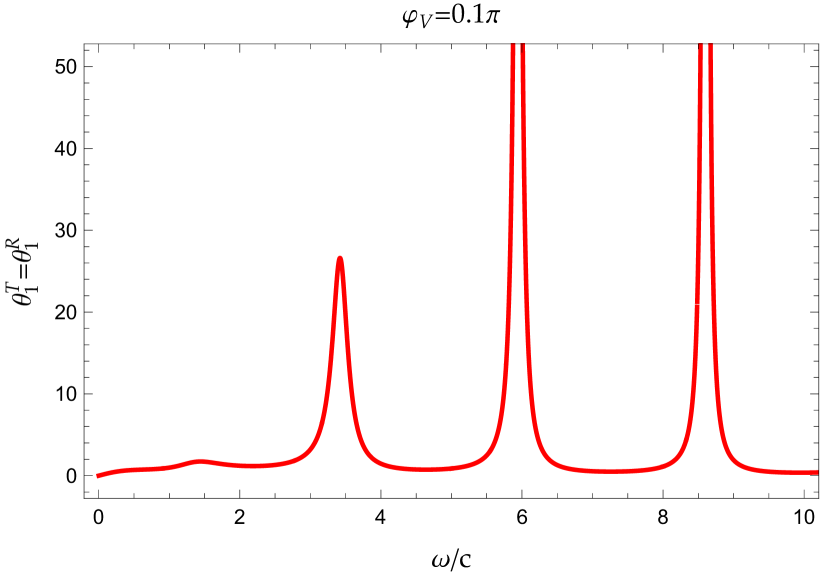
(a)

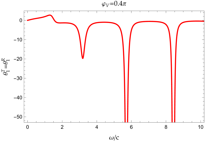
(b)

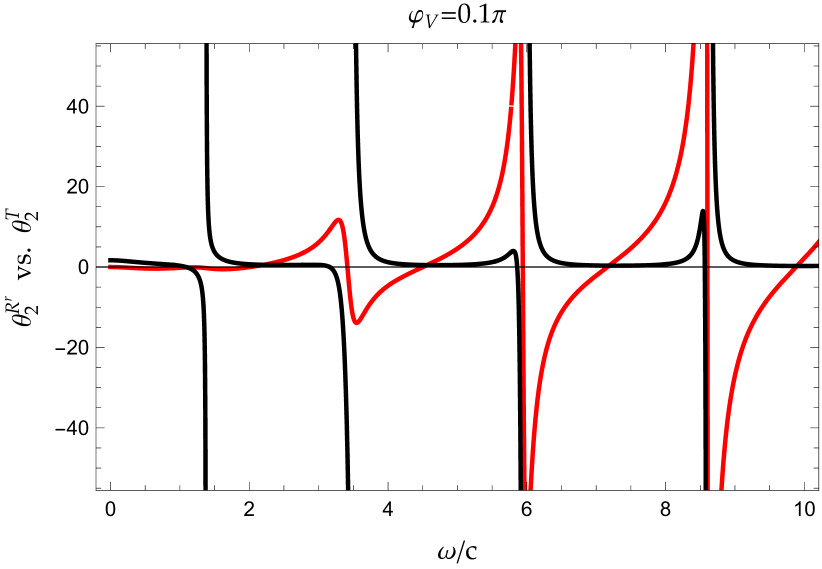
(c)

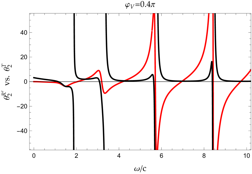
(d)

Figure 2: Faraday and Kerr rotation angles $\theta^{T}_{1,2}$ and $\theta^{R^{r}}_{1,2}$ versus $\frac{\omega}{c}$ are shown for two values of $\varphi_{V}=0.1\pi$ and $0.4\pi$ for $\mathcal{P}\mathcal{T}$-symmetric unite cell: (a) $\theta^{T}_{1}=\theta^{R}_{1}$ for $\varphi_{V}=0.1\pi$; (b) $\theta^{T}_{1}=\theta^{R}_{1}$ for $\varphi_{V}=0.4\pi$; (c) $\theta^{R^{r}}_{2}$ (solid red) vs. $\theta^{T}_{2}$ (solid black) for $\varphi_{V}=0.1\pi$; (d) $\theta^{R^{r}}_{2}$ (solid red) vs. $\theta^{T}_{2}$ (solid black) for $\varphi_{V}=0.4\pi$. The rest of parameters are taken as: $|V|=1$, $L=0.8$, $n=\sqrt{2}$ and $n_{0}=1$.

III.1 Spectral singularities in a unit cell

We now turn to a closer investigation of the spectral singularities for FR and KR angles. Spectral singularities are spectral points belonging to non-Hermitian Hamiltonian operators with $\mathcal{P}\mathcal{T}$-symmetry, characterized by real energies. At these energies, the reflection and transmission coefficients tend to infinity, i.e., they correspond to resonances having zero width. Interesting to note that a slight imbalance between gain and loss regions, can change the shape of the transition from zero width to the symmetric shape of the ”bell curve” (for more details see Ref. Gasparian et al. (2022a)).

For our model and for FR and KR rotational effects, spectral singularities arise when both conditions, $\mathcal{R}(\omega)=0$ and $\mathcal{I}(\omega)=0$, are satisfied simultaneously, see Eq.(15). By solving Eq.(15) for $\cot(kL)$ and $\omega$ one obtains straightforwardly

$$\bigg{(}\frac{\omega_{cr}|V|}{c}\bigg{)}^{2}\cos{2\varphi_{V}}+n^{2}+n^{2}_{0}=0,\ \ \ \ |V|=\sqrt{V_{1}^{2}+V_{2}^{2}},$$ (19)

where $\tan(\varphi_{V})=\frac{\mathcal{I}(\omega_{cr})}{\mathcal{R}(\omega_{cr})}$. The condition necessary for the existence of a solution of the spectral singularities exist only when the transmission phase is in the range $\varphi_{V}\in[\pi/4,\pi/2]$. Hence the critical value of $\omega_{cr}$ is defined as

$$\omega_{cr}=\frac{c}{|V|}\frac{\sqrt{n^{2}+n^{2}_{0}}}{\sqrt{|\cos{2\varphi_{V}}|}},$$ (20)

provided that

$$\cot\bigg{(}\frac{\omega_{cr}}{c}nL\bigg{)}=\frac{\sqrt{n^{2}+n_{0}^{2}}}{n}\frac{\cos{\varphi_{V}}}{\sqrt{|\cos{2\varphi_{V}}|}}.$$ (21)

For a fixed $|V|$, as follows from Eq.(20) the solutions of spectral singularities can only be found in a finite range: $\varphi_{V}\in[\frac{\pi}{4},\varphi_{c}]$, where $\varphi_{c}$ stands for upper bound of range. Hence as $\varphi_{V}$ approaches lower bound of range at $\frac{\pi}{4}$, the spectral singularity solution occurs at large frequency: $\omega\rightarrow\infty$. When $\varphi_{V}$ is increased, the solution of spectral singularity moves toward lower frequencies. As $\varphi_{V}$ approaches the upper bound of range at $\varphi_{c}$, the spectral singularity solution thus reaches its lowest value. The graphical illustration of the distribution of spectral singularities can be found in Fig.2 in Ref. Gasparian et al. (2022a).

III.2 Faraday and Kerr rotation: transmitted and reflected light

A phase transition-like anomalous behavior and properties of Faraday rotation angles in a simple $\mathcal{P}\mathcal{T}$-symmetric model with two complex $\delta$-potential placed at both boundaries of a regular dielectric slab was most recently reported in Ref.Gasparian et al. (2022a). Let us recall the essential features of the FR and then focus our attention on the KR effect. In a $\mathcal{P}\mathcal{T}$-symmetric systems a phase transition-like anomalous behavior of Faraday rotation angle take place. In this phase, one of Faraday rotation angles turns negative, and both angles yield strong enhancement near spectral singularities.

As the consequence of $\mathcal{P}\mathcal{T}$ symmetry constraint, the phase of reflected amplitude $\psi^{R}$ from left coincides with the phase of the transmission amplitude $\psi^{T}$, see Eq.(8). Hence the real part of the complex angle of KR, $\theta^{R}_{1}$, is always equal to the $\theta^{T}_{1}$ of FR, no matter what phase the system is in. In this sense, the situation is similar to the passive symmetric system, where is always $\theta^{R}_{1}=\theta^{T}_{1}$. It is interesting to note that Eq.(15) is invariant under the symmetry transform: $V_{2}\rightarrow-V_{2}$. This is a manifestation of the fact that the phase of reflected amplitude $\psi^{R}$ and as well as the Kerr rotation angle for the right incident light preserve the same behaviour, although the strengths of the right and left $\delta$-potentials on the boundaries are not equal to each other (more precisely, they are complex conjugate to each other). The mentioned asymmetry should lead to different left-to-right and right-to-left reflection amplitudes (see, e.g., Garmon et al. (2015)) and does not affect physical quantities $\theta^{R}_{1}$ and $\theta^{T}_{1}$, which are related to the phase accumulated during the process of reflection and transmission and as well as to the density of states. However, this asymmetry will affect $\theta^{R}_{2}$ and $\theta^{T}_{2}$, and they will no longer be equal to each other, see Fig. 2(c) and Fig. 2(d). This is consistent with the general statement that the Faraday and Kerr rotation profiles are very different from the corresponding curves describing ellipticities. In addition, symmetry constraint also yields the wavelength dependence of Faraday and Kerr ellipticity $\theta^{T}_{2}$ and $\theta^{R^{r/l}}_{2}$ shown in Eq.(11).

Here we would like to add a few more brief comments to emphasize that upon closer look at Fig.2 reveals some details of the similarities between curves that are relevant to our further discussion.

Firstly, the Faraday (Kerr) rotation local maximum/minimum (see Fig. 2) coincide with the local peak on the ellipticity curves with some accuracy. The ellipticity, at that frequencies, approaches zero non-linearly, becomes zero (linearly polarized light), and then the resulting polarization reverses its original direction.

Secondly, ellipticity (imaginary part the spectra) for $\theta^{T}_{2}$ and $\theta^{R}_{2}$ depend little on frequency and are close to zero in almost the entire frequency range, except for some regions associated with the maximum/minimum or spectral singularities of the Faraday rotation and Kerr rotation.

The questions discussed above can be straightforwardly generalized for the periodic $\mathcal{P}\mathcal{T}$-symmetric system. This will be done in the next section. We will show that the anomalous effect, similar to a phase transition, occurred more often due to the complex structure of the transmission and reflection amplitudes.

III.3 Limiting cases

The phase transition-like behavior of $\theta^{T}_{1}$ for two limiting cases $(|V|\rightarrow\infty$ and $V_{1}\rightarrow 0$) was discussed in Ref. Gasparian et al. (2022a). It was shown that in the case of $|V|\rightarrow\infty$ the sign of $\theta^{T}_{1}$ is completely determined by $\varphi_{V}$. As for the case $V_{1}=0$ ($\varphi_{V}\rightarrow\frac{\pi}{2}$), then again for the given parameters of the problem the anomalous negative behavior of $\theta^{T}_{1}$ is illustrated analytically. The latter case, that is a $\mathcal{P}\mathcal{T}$-symmetric optical lattice with a purely imaginary scattering potential has been discussed in detail in a number of investigations both theoretically and experimentally, see, e.g. Refs. Garmon et al. (2015) and references therein.

III.3.1 $|V|\rightarrow\infty$

The situation is slightly different for Kerr rotation. In the same limiting case $|V|\to\infty$, given that $\frac{n\omega L}{c}\neq\pi l$, we can show that $\theta^{R}_{2}\propto\frac{1}{|V|^{2}}$, hence the ellipticity is almost zero for all frequencies excluding $\frac{n\omega L}{c}=\pi l$ where $l\in\mathbb{Z}$ and the reflected light remains linearly polarized. At the discrete values of $\omega/c=\frac{\pi l}{nL}$ that yield the location of the resonance poles, $\theta^{R}_{2}$ display sharp peak with narrow resonance width. It reflects the fact that the reflected light is again linearly polarized but rotated 90 degrees from the initial direction.

III.3.2 $V_{1}\rightarrow 0$

Bound state solutions of the Schrödinger equation for a $\mathcal{P}\mathcal{T}$-symmetric potential with Dirac delta functions was study in Ref.Uncu and Demiralp (2006). In Ref.Gasparian et al. (2022a) it was pointed out that despite the fact that the expression for $\theta^{T}_{1}$ is valid for the case $V_{1}\rightarrow 0$, it can still explain not only the sign change of $\theta^{T}_{1}$ ($\theta^{R}_{1}$) in Fig.2 (a) where $V_{1}\neq 0$, but also explain existence first local maximum. It is clear that further features of the $\theta^{T}_{1}$ ($\theta^{R}_{1}$) in Fig. 3(a) near the frequencies of spectral singularities, is related to the behavior of $T(\omega)$.

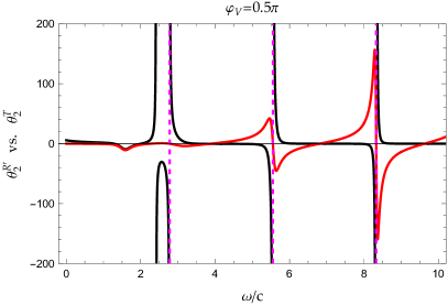
Figure 3: Plot of Faraday $\theta^{T}_{2}$ (solid red) and Kerr $\theta^{R^{r}}_{2}$ (solid black) rotation angles are shown for $|V|=1$, $\varphi_{V}=\frac{\pi}{2}$, $L=0.8$, $n=\sqrt{2}$ and $n_{0}=1$ for $\mathcal{P}\mathcal{T}$-symmetric unite cell, respectively. The resonant frequencies at $\frac{\omega_{l}n}{c}L=\pi l,\ l=1,2,\cdots$ are plotted as dashed pink vertical lines.

As for the imaginary portion of Kerr effect $\theta^{R^{r/l}}_{2}$, it is straightforward to show that in the same limit of $V_{1}\rightarrow 0$ the $\theta^{R^{r/l}}_{2}$ reads

$$\theta^{R^{r/l}}_{2}\stackrel{{\scriptstyle V_{1}\rightarrow 0}}{{\rightarrow}}\frac{g}{2nQ(\omega)}\left[\frac{1}{2}\bigg{(}\frac{1}{n_{0}}+\frac{n_{0}}{n^{2}}\bigg{)}\mp\frac{\omega}{cn^{2}}V_{2}\bigg{(}1\mp\frac{\omega}{2cn_{0}}V_{2}\bigg{)}+\frac{R^{r/l}_{0}}{Q^{r/l}(\omega)}\bigg{(}\frac{\omega L}{c}\frac{\cot(\frac{n\omega}{c}L)}{\sin^{2}(\frac{n\omega}{c}L)}-\frac{n^{2}-(n^{2}_{0}-\frac{\omega^{2}}{c^{2}}V^{2}_{2})^{2}}{4n^{2}_{0}n^{3}}\bigg{)}\right],$$ (22)

where the reflection coefficient $R^{r/l}_{0}$ is given by Eq.(14) and $Q^{r/l}(\omega)$ is defined by Eq.(18). The dependence of the imaginary part of the Kerr rotation $\theta^{R^{r}}_{2}$ (solid black line) on $\frac{\omega}{c}$ for $V_{1}\rightarrow 0$ is illustrated in Fig. 3. A number of basic features of $\theta^{R}_{2}$ can be observed even in this simplest case of $V_{1}\rightarrow 0$. One of the key features is the single resonant peak that show up clearly when $R_{0}\rightarrow\infty$, see Eq.(22). As mentioned above the resonance frequencies are spectral singularities when both conditions, ${\it\mathcal{R}}(\omega)=0$ and ${\it\mathcal{I}}(\omega)=0$, are satisfied simultaneously. In the particular case of $V_{1}\rightarrow 0$ there is only one $\omega_{cr}$ that can be directly calculated from Eq.(20) by putting $\varphi_{V}=\frac{\pi}{2}$: $\omega_{cr}=\frac{c\sqrt{n^{2}+n^{2}_{0}}}{V_{2}}$. The second condition $\cot\bigg{(}\frac{\omega_{cr}}{c}nL\bigg{)}=0$ can be satisfied by choosing the appropriate value of length is $L=0.8$ (the system parameters are: $n_{0}=c=V_{2}=1$, $n=\sqrt{2}$ and $\omega_{cr}=\sqrt{3}$). Other maxima or minima in the Kerr rotation, located near the resonant frequencies, are associated with multiple reflections from the boundaries and are located at $\frac{\omega_{l}n}{c}L=\pi l,\ l=1,2,\cdots$ (see vertical pink lines in Fig.3).

Repeating similar calculations leading to Eq.(22), we arrive at an explicit expression for ellipticity $\theta^{T}_{2}$ for Faraday rotation for this simplest case with a purely imaginary potential:

$$\theta^{T}_{2}\stackrel{{\scriptstyle V_{1}\rightarrow 0}}{{\rightarrow}}\frac{g}{2n}{\cot(kL)}\frac{\omega}{c}L\left[T_{0}\left(1-\frac{{\sin^{2}(kL)}}{\cot(kL)}\frac{c}{\omega L}\frac{n^{2}-(n^{2}_{0}-\frac{\omega^{2}}{c^{2}}V^{2}_{2})^{2}}{4n^{2}_{0}n^{3}}\right)-1\right].$$ (23)

We observe that the smoothed maxima and minima that appeared around the zeros of $\sin{kL}$ at $\frac{\omega_{l}n}{c}L=\pi l,\ l=1,2,\cdots$ coincides with maxima and minima of $\theta^{R}_{2}$ and associated with multiple reflections from the boundaries, see e.g. vertical yellow lines in Fig.3. Secondly, the large value of $\theta^{T}_{2}$ at $3\pi/2$ is related to the frequency of the spectral singularity $\omega_{cr}=\frac{c\sqrt{n^{2}+n^{2}_{0}}}{V_{2}}$, where $T_{0}\rightarrow\infty$.

The physical background of the relatively simple mathematical structure of the Faraday rotation angle $\theta^{T}_{1}$ on the frequency of comparison Kerr ellipticity ($\theta^{R^{r/l}}_{2}$ is that in the first case the rotation maximum is direct proportional to the optical anisotropy (for example, the larger ( $n_{+}-n_{-}$ ), the larger is $\theta^{T}_{1}$. However, the maximisation of $\theta^{R^{r/l}}_{2}$ is, not so straightforward, since anisotropy indices are mixed (see, e.g, Ref. Němec et al. (2018) and and references therein).

IV Periodic system with $2N+1$ cells

It is known that when the wave propagation through a medium is described by a differential equation of second order, the expression for the total transmission from the finite periodic system for any waves (sound and electromagnetic) depends on the unit cell transmission, the Bloch phase and the total number of cells. As an example of collective interference effect, let us mention the intensity distribution from $N$ slits (diffraction due to $N$-slits), as well as the formula that describes the Landauer’s resistance of a one-dimensional chain of periodically spaced $N$ random scatterers. In both cases, the similarity of the results is obvious. However, the physics behind these results is completely different both in spirit and in details. In analogy to Hermitian Hamiltonian, one can expect interference effect holds also for a non-Hermitian Hamiltonian system. In this sense it is a natural result for a $\mathcal{P}\mathcal{T}$-symmetric system that a somewhat similar formula for transmission and reflection amplitudes appears, for example, in Refs. Achilleos et al. (2017); Kalozoumis et al. (2018); Lin et al. (2011a); Guo et al. (2022). The infinite periodic $\mathcal{P}\mathcal{T}$-symmetric structures, because of unusual properties, including the band structure, Bloch oscillations, unidirectional propagation and enhanced sensitivity, are of special interest and are presently the subject of intensive ongoing research (see e.g., Refs. Bender et al. (1999); Shin (2004); Musslimani et al. (2008); Midya et al. (2010) and references therein). However, the case of scattering in a finite periodic systems composed of an arbitrary number of cells/scatters has been less investigated, despite that any open quantum systems generally consist of a finite system coupled with an infinite environment.

In many studies, to describe quantitatively, both amplification and absorption in periodic $\mathcal{P}\mathcal{T}$-symmetric systems, the transfer matrix method is used. The latter, can be reduced to the evolution of the product of transfer matrices of complex, but identical unit cells, and using the classical Chebyshev identity get the final result.

In the following, we present the amplitudes of transmission and reflection form the left and right sides of the incident wave based on the characteristic determinant approach, the technical details are given in Appendix A. The latter, in principle, is compatible with the transfer matrix method and is convenient for both numerical and analytical calculations.

IV.1 Amplitudes of transmission and reflection form left and right

We now turn to a closer investigation of the Faraday and Kerr rotations for various parameter ranges of our $\mathcal{P}\mathcal{T}$-periodic symmetric system that consists of $2N+1$ cells, see Fig.1. Following Refs. Gasparian et al. (1997); Guo et al. (2022) and also see Appendix A, a generic expressions for the transmission and left/right reflection amplitudes for the $\mathcal{P}\mathcal{T}$ can be presented as:

$$t(\omega) =\frac{e^{-ik_{0}L_{0}}}{\cos(\beta(2N+1)\Lambda)+iIm\left[\frac{e^{-ik_{0}L_{0}}}{t_{0}(\omega)}\right]\frac{\sin(\beta(2N+1)\Lambda)}{\sin(\beta\Lambda)}},$$ (24)

where $k_{0}=n_{0}\frac{\omega}{c}$ and $k=n\frac{\omega}{c}$ are the wave vectors in the respective medium. The quasi-momentum $\beta$ is the Bloch wave vector of the infinite periodic system with unit cell length or spatial periodicity $\Lambda=L_{0}+L$:

$$\cos({\beta\Lambda})\equiv{\it Re}\left[\frac{e^{-ik_{0}L_{0}}}{t_{0}(\omega)}\right]=\sin(kL)\left[\cos(k_{0}L_{0})\mathcal{R}(\omega)-\sin(k_{0}L_{0})\mathcal{I}(\omega)\right].$$ (25)

please confirm two equations in blue. The left/right reflection amplitude can be written in the form Guo et al. (2022); Gasparian et al. (1997)

$$\frac{r^{(r/l)}(\omega)}{t(\omega)} =\left[\frac{r^{(r/l)}_{0}(\omega)}{t_{0}(\omega)}\right]\frac{\sin(\beta(2N+1)\Lambda)}{\sin(\beta\Lambda)},$$ (26)

where $t_{0}(\omega)$ and ${r^{(r/l)}_{0}(\omega)}$ are the transmission and reflection amplitudes for a single cell ($N=0$) that are given in Eq.(14) and Eq.(17) respectively.

An important feature of expressions (24) and (26) is that both contain factor $\frac{\sin(\beta(2N+1)\Lambda)}{\sin(\beta\Lambda)}$ which naturally occur in Hermitian one-dimensional finite periodic systems due to interference or diffraction effects and reflects a combine effect of all $2N+1$ cell. The appearance of this factor in non-Hermitian systems is highly non-trivial from the view of the usual probability conservation property for Hermitian systems (the reflection and transmission coefficients must sum to unit in either classical or quantum mechanical regimes) or unitary scattering matrix theory. However, in Refs. Achilleos et al. (2017); Guo et al. (2022) a simple closed form expressions is obtained for the total transmission and reflection (left/right) amplitudes from a lattice of $N$ cells. As pointed out in Refs. Guo et al. (2022), the transmission and reflection amplitudes for a periodic many scatters system are related to single cell amplitudes in a compact fashion. This is intimately connected with the fact that the factorization of short-range dynamics in a single cell and long-range collective effect of periodic structure of entire system: the short-range interaction dynamics that is described by single cell scattering amplitudes and the $\beta$ represents the collective mode of entire lattice. The occurrence of factorization of short-range dynamics and long-range collective mode has been known in both condensed matter physics and nuclear/hadron physics. In the cases such as particles interacting with short-range potential in a periodic box or trap, where two physical scales, (1) the short-range particles dynamics and (2) long-range geometric effect due to the periodic box or trap, are clearly separated. The quantization conditions are given by a compact formula that is known as Korringa–Kohn–Rostoker (KKR) method Korringa (1947); Kohn and Rostoker (1954) in condensed matter physics, Lüscher formula Lüscher (1991) in LCQD and Busch-Englert-Rzażewski-Wilkens (BERW) formula Busch et al. (1998) in a harmonic oscillator trap in nuclear physics community. Other related useful discussions can be found in e.g. Refs.Guo and Long (2022); Guo and Gasparian (2021, 2022b); Guo (2021).

Above statement can also be demonstrated by the expression of transmission coefficient $T=|t|^{2}$ for the finite system with $2N+1$ cells,

$$\frac{1}{T}=1+{\frac{r_{0}^{r}}{t_{0}}}{\frac{{r_{0}^{l}}^{*}}{{t_{0}}^{*}}\frac{\sin^{2}(\beta(2N+1)\Lambda)}{\sin^{2}(\beta\Lambda)}}=1+\bigg{(}\frac{1}{T_{0}}-1\bigg{)}\frac{\sin^{2}(\beta(2N+1)\Lambda)}{{\sin^{2}(\beta\Lambda)}}.$$ (27)

In addition, Equation (27) shows that there are two distinct cases for which an incident wave is totally transmitted, i.e. $T=1$. This implies perfect resonant transmission with no losses and no gain, regardless of the complex nature of the coupling constants.

The first case occurs when there is no reflected wave from any individual cell and this matches the condition when the product of $\frac{r_{0}^{r}}{t_{0}}\frac{{r_{0}^{l}}^{*}}{{t_{0}}^{*}}$ in Eq. (27) is zero (or $T_{0}=1$). This would lead to the unidirectional propagation discussed in several studies on $\mathcal{P}\mathcal{T}$-symmetric systems, see, e.g, Refs. Lin et al. (2011b); Feng et al. (2013); Longhi (2011); Longhi and Della Valle (2013). This phenomenon is also referred as the effect of exceptional points (EPs) that separate the broken and unbroken $\mathcal{P}\mathcal{T}$-symmetric phases, see e.g. Refs. El-Ganainy et al. (2018); Bender et al. (2019); Miri and Alù (2019); Özdemir et al. (2019).

In the second case $\sin(\beta(2N+1)\Lambda)/\sin(\beta\Lambda)=0$. It corresponds to constructive interference between path reflected from different unit cells at

$${\beta\Lambda}={\frac{\pi l}{2N+1}},\qquad|l|=1,\cdots,N.$$ (28)

In both cases mentioned, we have a perfect transmission, that is, $T=1$. As a consequence, the product of two the reflection coefficients on the left and right should disappear according to the formula (9). In the case, when one of reflections reach zero while the other remains non-zero, so-called unidirectional transparency can occur when we have an ideal non-reflective transmission in one direction but not in the other. The experimental demonstration of a unidirectional reflectionless at optical parity-time metamaterial at optical frequencies is reported in Ref. Feng et al. (2013). An outlook on the potential directions and applications of controlling sound in non-hermitian acoustic systems can be found in Ref.Gu et al. (2021).

IV.2 Spectral singularities in periodic system with $2N+1$ cells

To illustrate the influence of the two factors mentioned above, as well as the role of spectral singularities on the formation of Faraday and Kerr rotations and their shapes let us note that (i) the spectral singularities arise when both conditions, $\it Re(\omega)=0$ and $Im(\omega)=0$, are satisfied simultaneously (ii) the location of these poles can be found by solving $1/t(k)=0$. Based on Eq.(24), there are two types of solutions, as was mentioned above:

(i) Type I singularities are given by solutions of $\frac{1}{t_{0}(\omega)}=0$. Hence $\cos(\beta\Lambda)=0$ and $\frac{1}{t(\omega)}=0$ are both automatically satisfied:

$$\beta\Lambda=\pi l+\frac{\pi}{2},\ \ \ \ l\in\mathbb{Z}.$$ (29)

The type I singularities are originated from a single cell ($N=0$), and shared by the entire system of $2N+1$ cells. The type I solutions are independent of number of cells and the size of system. The detailed discussion about type I singularities can be found in Sec.III.1.

(ii) type II singularities depend on the size of the system and are given by two conditions,

$$\cos\left(\beta(2N+1)\Lambda\right)=0,\ \ \ \ Im\left[\frac{e^{-ik_{0}L_{0}}}{t_{0}(k)}\right]=0.$$ (30)

Hence $\beta\Lambda=\frac{\pi(l+\frac{1}{2})}{2N+1}$ where $l\in\mathbb{Z}$, above two conditions are given explicitly by

$$\sin\left(\frac{n\omega_{cr}}{c}L\right)\left[\cos\left(\frac{n_{0}\omega_{cr}}{c}L_{0}\right)\mathcal{R}(\omega_{cr})-\sin\left(\frac{n_{0}\omega_{cr}}{c}L_{0}\right)\mathcal{I}(\omega_{cr})\right] =\cos\frac{\pi(l+\frac{1}{2})}{2N+1},$$

$$\cos\left(\frac{n_{0}\omega_{cr}}{c}L_{0}\right)\mathcal{I}(\omega_{cr})+\sin\left(\frac{n_{0}\omega_{cr}}{c}L_{0}\right)\mathcal{R}(\omega_{cr}) =0.$$ (31)

At the limit of $V_{1}\rightarrow 0$, two conditions are reduced to

$$\frac{V^{2}_{2}\omega^{2}_{\omega_{cr}}}{2c^{2}nn_{0}}-\tan\left(\frac{n_{0}\omega_{cr}L_{0}}{c}\right)\cot\left(\frac{n\omega_{cr}L}{c}\right)=\frac{1}{2}\left(\frac{n_{0}}{n}+\frac{n}{n_{0}}\right),\ \ \ \cos\frac{\pi(l+\frac{1}{2})}{2N+1}=\frac{\cos\left(\frac{n\omega_{cr}L}{c}\right)}{\cos\left(\frac{n_{0}\omega_{cr}L_{0}}{c}\right)}$$ (32)

IV.3 Large $N$ limit

As number of cells is increased, all FR and KR angles demonstrate fast oscillating behavior due to $\sin(\beta(2N+1)\Lambda)$ and $\cos(\beta(2N+1)\Lambda)$ functions in transmission and reflection amplitudes. These behaviors are very similar to what happens for tunneling time of a particle through layers of periodic $\mathcal{P}\mathcal{T}$-symmetric barriers that is discussed in Ref. Guo et al. (2022). For the large $N$ systems, we can introduce the FR and KR angles per unit cell

$$\widehat{\theta}^{T/R}(\omega)=\frac{\theta^{T/R}(\omega)}{(2N+1)\Lambda}.$$ (33)

The $N\rightarrow\infty$ limit may be approached by adding a small imaginary part to $\beta$: $\beta\rightarrow\beta+i\epsilon$, where $\epsilon\gg\frac{1}{(2L+1)\Lambda}$. As discussed in Ref. Guo et al. (2022), adding a small imaginary part to $\beta$ is justified by considering the averaged FR and KR angles per unit cell, which ultimately smooth out the fast oscillating behavior of FR and KR angles. Using asymptotic behavior of

$$\sec(\beta(2N+1)\Lambda)\propto 2e^{i\beta(2N+1)\Lambda},\ \ \ \ \tan(\beta(2N+1)\Lambda)\propto 1,$$ (34)

we find

$$\frac{1}{(2N+1)\Lambda}\ln t(\omega)\stackrel{{\scriptstyle N\rightarrow\infty}}{{\rightarrow}}i\beta,\ \ \ \ \frac{1}{(2N+1)\Lambda}\ln r(\omega)\stackrel{{\scriptstyle N\rightarrow\infty}}{{\rightarrow}}0.$$ (35)

Therefore, as $N\rightarrow\infty$, FR and KR angles per unit cell approach

$$\widehat{\theta}^{T}_{1}\stackrel{{\scriptstyle N\rightarrow\infty}}{{\rightarrow}}-\frac{g}{2n}\frac{\partial Re[\beta]}{\partial n},\ \ \ \ \widehat{\theta}^{T}_{2}\stackrel{{\scriptstyle N\rightarrow\infty}}{{\rightarrow}}\frac{g}{2n}\frac{\partial Im[\beta]}{\partial n},\ \ \ \ \widehat{\theta}^{R^{r/l}}_{1,2}\stackrel{{\scriptstyle N\rightarrow\infty}}{{\rightarrow}}0.$$ (36)

Also noted that at large $N$ limit,

$$\sin(\beta(2N+1)\Lambda)\propto-\frac{1}{2i}e^{-i\beta(2N+1)\Lambda}\stackrel{{\scriptstyle N\rightarrow\infty}}{{\rightarrow}}\infty,$$ (37)

using Eq.(27), one can show that transmission coefficient therefore approaches zero: $T\stackrel{{\scriptstyle N\rightarrow\infty}}{{\rightarrow}}0$. The relation between $\widehat{\theta}^{T}_{2}$ and $\widehat{\theta}^{R^{r/l}}_{2}$ given in Eq.(11) hence is still valid as $N\rightarrow\infty$.

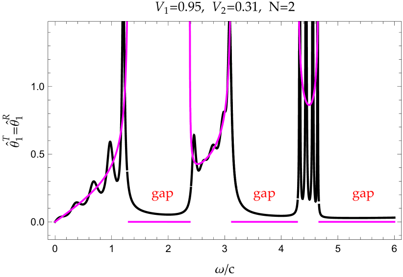
(a)

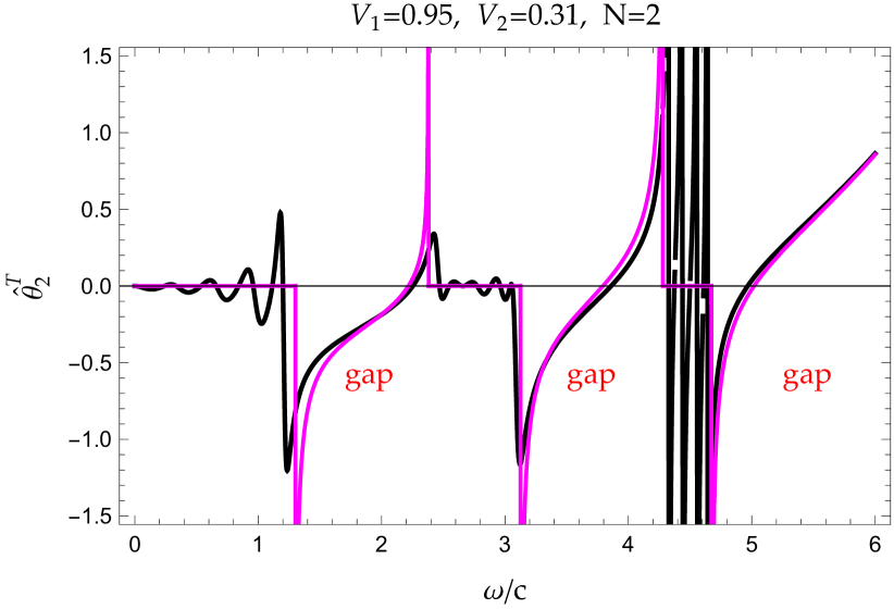
(b)

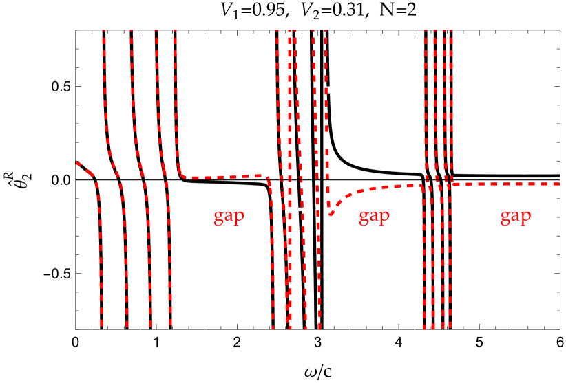
(c)

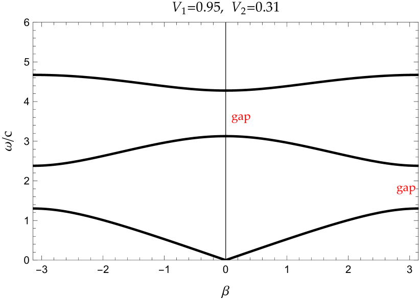
(d)

Figure 4: Plot of FR and KR angles with $N=2$ vs. large $N$ limit result: $i\frac{g}{2n}\frac{d\beta}{dn}$ (solid purples): (a) $\widehat{\theta}^{T}_{1}=\widehat{\theta}^{R}_{1}$ (solid black) vs. $\frac{g}{2n}\frac{dRe[\beta]}{dn}$ (solid purple); (b) $\widehat{\theta}^{T}_{2}$ (solid black) vs. $-\frac{g}{2n}\frac{dIm[\beta]}{dn}$ (solid purple); (c) $\widehat{\theta}^{R^{r}}_{2}$ (solid black) vs. $\widehat{\theta}^{R^{l}}_{2}$ (dashed red); (d) Band structure plot in unbroken phase. The parameters are taken as: $V_{1}=0.31$, $V_{2}=0.95$, $L=0.2$, $L_{0}=0.8$, $n=2$ and $n_{0}=1$

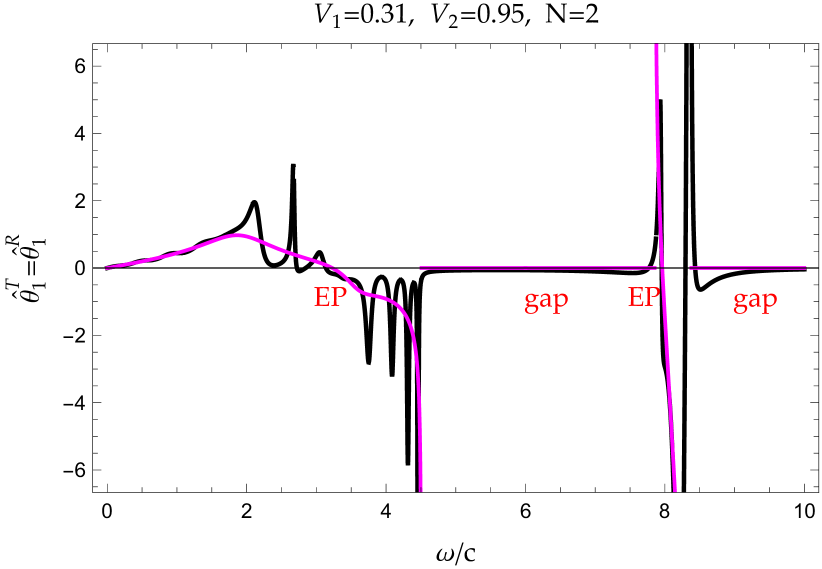
(a)

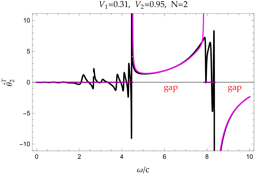
(b)

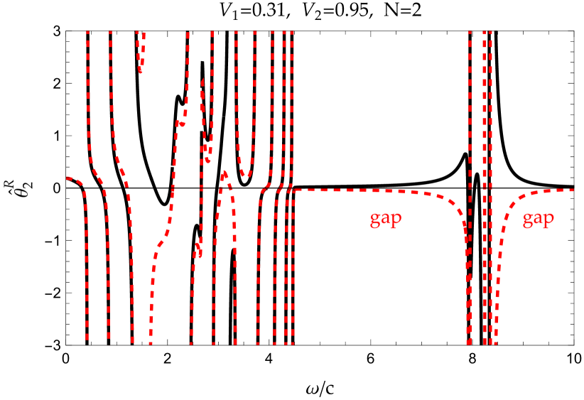
(c)

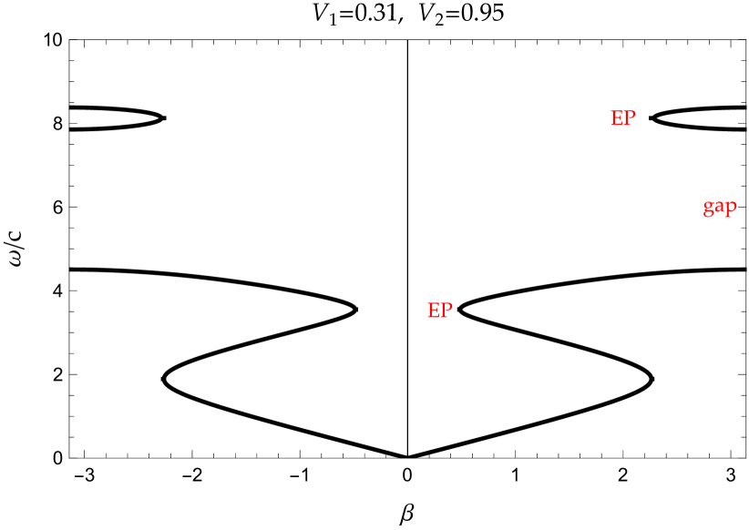
(d)

Figure 5: Plot of FR and KR angles with $N=2$ vs. large $N$ limit result: $i\frac{g}{2n}\frac{d\beta}{dn}$ (solid purples): (a) $\widehat{\theta}^{T}_{1}=\widehat{\theta}^{R}_{1}$ (solid black) vs. $\frac{g}{2n}\frac{dRe[\beta]}{dn}$ (solid purple); (b) $\widehat{\theta}^{T}_{2}$ (solid black) vs. $-\frac{g}{2n}\frac{dIm[\beta]}{dn}$ (solid purple); (c) $\widehat{\theta}^{R^{r}}_{2}$ (solid black) vs. $\widehat{\theta}^{R^{l}}_{2}$ (dashed red); (d) Band structure plot in broken phase. The parameters are taken as: $V_{1}=0.31$, $V_{2}=0.95$, $L=0.2$, $L_{0}=0.8$, $n=2$ and $n_{0}=1$.

The examples of FR and KR angles per unit cell for a$\mathcal{P}\mathcal{T}$-symmetric finite system with five cells are shown in Fig. 4 and Fig. 5, compared with the large $N$ limit results. As we can see in Fig. 4 and Fig. 5, the $\theta^{T}_{1}$ and $\theta^{T}_{2}$ angles oscillating around the large $N$ limit results. Even for the small size system, we can see clearly that the band structure of infinite periodic system is already showing up. The oscillating KR angles are consistent with zero at large $N$ limit. In addition, in broken $\mathcal{P}\mathcal{T}$-symmetric phase in Fig. 5, EPs can be visualized even for a small size system, where two neighbouring bands merge and the $\mathcal{P}\mathcal{T}$ becomes totally transparent: both $\theta^{T}_{1}$ and $\theta^{T}_{2}$ approach zero.

For a real refractive index profile, the sign of $\theta^{T}_{1}$ is always positive due to the fact that $\theta^{T}_{1}$ is closely related to the density of states. However, in $\mathcal{P}\mathcal{T}$-symmetric systems, $\theta^{T}_{1}$ is now associated with a generalized density of states, which can be either positive or negative, see discussion in Ref.Guo et al. (2022); Guo and Gasparian (2022a). In this sense the negative spike(s) in Fig. 4 and Fig. 5 around the some frequencies provide the formal justification of the existence of such negative states. Turning negative of $\theta^{T}_{1}$ is closely related to the motion of poles across the real axis moving from unphysical sheet (the second Riemann sheet) into physical sheet (the first Riemann sheet), for more details see Refs.Guo et al. (2022); Gasparian et al. (2022b). Since $\theta^{T}_{1}$ ($\theta^{R}_{1}$) is assumed to be related to the density of states, it is natural that it is practically zero in all forbidden bands and takes a giant leap to a very large number at the end of each band.

V Discussion and summary

In summary, we studied the anomalous behavior of the Faraday (transmission) and polar Kerr (reflection) rotation angles of the propagating light, in finite periodic parity-time ($\mathcal{P}\mathcal{T}$) symmetric structures, containing $2N+1$ cells.

We have obtained closed form expressions for FR and KR angles for a single cell consisting of two complex $\delta$-potentials placed on both boundaries of the ordinary dielectric slab. It is shown that, for a given set of parameters describing the system, a phase transition-like anomalous behavior of Faraday and Kerr rotation angles in a parity-time symmetric systems can take place. In the anomalous phase the value of one of the Faraday and Kerr rotation angles can become negative, and both angles suffer from spectral singularities and give a strong enhancement near the singularities. It is shown that due to symmetry constraints, the real part of the complex angle of KR, $\theta^{R}_{1}$, is always equal to the $\theta^{T}_{1}$ of FR, no matter what phase the system is in. The imaginary part of KR angles $\theta^{R^{r/l}}_{2}$ are also related to the $\theta^{T}_{2}$ of FR by parity-time symmetry.

We find that, in the limit of weak scattering, the Kerr and Faraday rotation angles increase linearly with the length of the system. In this approximation the effects of multiple reflections within the layers are not significant. We have also shown, based on the modified Kramers-Kronig relations, that only the three angles FR and KR are completely independent.

Appendix A Determinant Approach

This section is devoted to more mathematical interest. We combine two non-perturbative approaches, that sufficiently completely describe of photon (electron) behaviour in a random potential to study the energy spectrum and scattering matrix elements in the $\mathcal{P}\mathcal{T}$ system without actually determining the photon eigenfunctions.

In both approaches, the Green’s function was calculated exactly for two different models. In the first model, we are dealing with the sum of $\delta$-potentials distributed randomly with an arbitrary strength. The second model was used to calculate the passage of a free particle through a layered system, which is characterized by random parameters of the layers.

A convenient formalism to study one dimensional scattering systems satisfying the stationary Schrödinger equation or the Helmholtz equation relevant to optical Bragg grating is developed in Ref Aronov et al. (1991); Gasparyan (1989). The approach allows one to express the transmission and reflection amplitudes of a wave propagating in a one-dimensional random layered structure through the characteristic determinant $D_{N}$ ($N$ is the number of the boundaries), which depends on the amplitudes of reflection of a single scatter only. The transmission amplitude $t_{N}$ of waves through the systems can be presented in the form

$$t_{N}=\frac{e^{ik|x_{N}-x_{1}|}}{D^{0}_{N}},$$ (38)

where the characteristic determinant $D^{0}_{N}$ reduces to a recursive equation that is convenient for both numerical and analytical approaches.

This paper presents a generalization of the determinant approach to the case of $\mathcal{P}\mathcal{T}$-symmetric (non-symmetric) systems consisting of $(N-1)$ dielectric multilayers with two delta potentials in each. The detailed and, in many respects, complete description and analysis of the Faraday and Kerr effects in such a system discussed. Specifically, our investigations focus on the periodic finite size diatomic $\mathcal{P}\mathcal{T}$-symmetric model. We predict that for a given set of parameters describing the system the Faraday and Kerr rotation angles show a non-trivial transition with a change in sign. In the anomalous phase the value of one of the Faraday and Kerr rotation angles can become negative, and both angles suffer from spectral singularities and give a strong enhancement near the singularities.

Let us consider $(N-1)$ dielectric multilayer system labeled $n={1,\cdots,N-1}$ between two semi-infinite media. The positions of the boundaries of the $nth$ dielectric layer, characterized by the constant $\epsilon_{n}$, are given by $x_{n}$ and $x_{n+1}$ respectively. The left and right ends of the system are at $x=x_{{}_{N}}$ and $x=x_{1}$ with $\epsilon_{0}=\epsilon_{N}$, respectively. We assume that a plain EMW wave is incident from the left (with the dielectric permittivity $\epsilon_{0}$) onto the boundary at $x=x_{1}$ and evaluate the amplitude of the reflected wave and the wave propagating in the semi-infinite media for $x>x_{N}$, characterized by $\epsilon_{N}$. In the further discussion we will assume, that the first and last layers of the multilayer system make interfaces with the vacuum.

We also assume that we know the transmission $t_{n,n+1}$ and reflection amplitudes (from the left $r_{n,n+1}$ and the right $r_{n+1,n}$) of the EMW from a single $Z_{n}\delta(x-x_{n})$ scatter, located at the contact of two semi-infinite media I and II at $x=x_{n}$. Using the results of the transmission and reflection amplitudes for the single scatter, we will build characteristic determinant $D_{N}$ for $N$ scatters and obtain the total transmission $t_{N}$ and reflection amplitudes $r^{N}_{L}$ and $r^{N}_{R}$. The transmission amplitudes from left and from right equal each other are given by

$$t_{n,n+1}=t_{n+1,n}\equiv\frac{2\sqrt{\frac{k_{n}}{k_{n-1}}}}{1+\frac{k_{n}}{k_{n-1}}-i\frac{\gamma}{k_{n-1}}Z_{n}},\ \ \ \ k_{n}=\frac{\omega}{c}n,\ \ \ \ \gamma\equiv\left(\frac{\omega}{c}\right)^{2}.$$ (39)

Similarly,

$$r_{n,n+1}=\frac{1-\frac{k_{n+1}}{k_{n}}+i\frac{\gamma}{k_{n}}Z_{n}}{1+\frac{k_{n+1}}{k_{n}}-i\frac{\gamma}{k_{n}}Z_{n}},\ \ \ \ r_{n+1,n}=\frac{\frac{k_{n+1}}{k_{n}}-1+i\frac{\gamma}{k_{n}}Z_{n}}{1+\frac{k_{n+1}}{k_{n}}-i\frac{\gamma}{k_{n}}Z_{n}}.$$ (40)

We can easily verify by using Eq.(39) and Eq.(40) that the conservation law is satisfied, provided that $Z_{n}$ is real:

$$t_{n,n+1}t^{*}_{n,n+1}+r_{n,n+1}r^{*}_{n,n+1}=\frac{4\frac{k_{n}}{k_{n-1}}+(1-\frac{k_{n}}{k_{n-1}})^{2}+(\frac{\gamma}{k_{n-1}}Z_{n})^{2}}{(1+\frac{k_{n}}{k_{n-1}})^{2}+(\frac{\gamma}{k_{n-1}}Z_{n})^{2}}=1$$ (41)

In the case of a complex value $Z_{n}$, the conservation law cannot hold, since the system is not $\mathcal{P}\mathcal{T}$-symmetric and can be described by only complex energy eigenvalue. Later, when we ”build” the characteristic determinant $D_{N}$ for the entire system with $N$ complex potentials, distributed arbitrary, we will return to the conservation law of the system in more detail.

Assuming that we know the explicit expression for the amplitude of reflection from a single-scattering delta potential, see Eq.(40), we now turn to a closer investigation of the system with two complex potentials. Following Refs.Aronov et al. (1991), we can present the determinant $D_{2}$ of two delta potentials located at points $x_{1}$ and $x_{2}$ ($L$ = $x_{2}$- $x_{1}$) on the left and right boundaries of a dielectric slab surrounded by two semi-infinite media with permittivities $\epsilon_{0}$ (left) and $\epsilon_{2}$ (right), respectively. The dielectric slab itself is characterized by permittivity $\epsilon_{1}$. The explicit form of $D_{2}$ is

$$D^{0}_{2}=\frac{1}{(1+r_{21})(1+r_{32})}\det D_{2},$$ (42)

where

$$\det D_{2}\equiv\begin{vmatrix}1&r_{23}e^{ik_{1}(x_{2}-x_{1})}\\ r_{21}e^{ik_{1}(x_{2}-x_{1})}&1\end{vmatrix},$$ (43)

and $r_{n,n+1}$ is given by Eq.(40) with the appropriate choice of $n$ and $Z_{n}$. Let us add another boundary from the right, at the point $x_{3}$, i.e. we consider a layered heterostructure consisting of two films with permittivities $\epsilon_{1}$ and $\epsilon_{2}$, placed between two semi-infinite media $\epsilon_{0}$ and $\epsilon_{3}$.

Next, adding another delta complex potential $Z_{3}$ at $x_{3}$ the new $D_{3}$, which now is $3\times 3$ determinant, can be written as

$$D^{0}_{3}= \prod^{3}_{l=1}\frac{1}{(1+r_{l+1,l})}\det D_{3}$$ (44)

where

$$\det D_{3}\equiv\begin{vmatrix}1&r_{23}e^{ik_{1}(x_{2}-x_{1})}&r_{34}e^{ik_{1}(x_{2}-x_{1})}e^{ik_{2}(x_{3}-x_{2})}\\ r_{21}e^{ik_{1}(x_{2}-x_{1})}&1&r_{34}e^{ik_{2}(x_{3}-x_{2})}\\ r_{21}e^{ik_{1}(x_{2}-x_{1})}e^{ik_{2}(x_{3}-x_{2})}&r_{32}e^{ik_{2}(x_{3}-x_{2})}&1\\ \end{vmatrix}.$$ (45)

By continuing adding new boundaries and complex potential $Z_{n}$ at the points $x_{4}$,…, $x_{N}$, we will obtain an $N$-multilayer system, each layer of which contains two delta potentials. This system will be characterized by the product of $N$ by $N$ determinant $D_{N}$

$$D^{0}_{N}=\prod^{N}_{l=1}\frac{1}{(1+r_{l+1,l})}\det D^{N}_{l,n},$$ (46)

with the following matrix elements $D^{N}_{l,n}$:

$$D^{N}_{l,n}=\left\{\begin{array}[]{l l}\delta_{ln}+(1-\delta_{ln})r_{l,l-1}e^{ik_{l}|x_{l}-x_{n}|},\ \ l\geq n,\\ \delta_{ln}+(1-\delta_{ln})r_{l-1,l}e^{ik_{l}|x_{l}-x_{n}|},\ \ n\geq l.\\ \end{array}\right.$$ (47)

The characteristic determinant $D_{N}$ can be presented as a determinant of a Teoplitz tridiagonal matrix that satisfies the following recurrence relationship:

$$D_{N}=A_{N}D_{N-1}-B_{N}D_{N-2},$$

where $D_{N-1}$ ($D_{N-2}$) is the determinant equation (47) with the $Nth$ and also the $(N-1)th$ row and column omitted. The initial conditions for the recurrence relations are $D_{0}=1$, $D_{-1}=0$, $D_{1}\equiv A_{1}=1$. The coefficients $A_{N}$, $B_{N}$ can be obtained from the explicit form of $D^{N}_{n,l}$ (see Eq. (47)). For $N>1$ we have

$$A_{n}=1+\frac{r_{n,n+1}}{r_{n-1,n}}(1+r_{n-1,n}+r_{n,n-1})e^{2ik_{n}|x_{n}-x_{n-1}|}=1+B_{n}-r_{n,n-1}r_{n,n+1}e^{2ik_{n}|x_{n}-x_{n-1}|}$$

and

$$B_{n}=\frac{r_{n,n+1}}{r_{n-1,n}}(1+r_{n,n-1})(1+r_{n-1,n})e^{2ik_{n}|x_{n}-x_{n-1}|}$$

In concluding, let us stress once more that Eqs.(46) and (47) may be viewed as generalization of the characteristic determinant method that can be applied to the Helmholtz (Shrödinger) equation with complex potentials, distributed arbitrary and find scattering matrix elements without actually determining the photon (electron) eigenfunctions.

References

- Yoshino (2005) T. Yoshino, Journal of the Optical Society of America B Optical Physics 22, 1856 (2005).
- Zamani et al. (2011) M. Zamani, M. Ghanaatshoar, and H. Alisafaee, Journal of the Optical Society of America B Optical Physics 28, 2637 (2011).
- Birch (1982) K. P. Birch, Optics Communications 43, 79 (1982).
- Corzo et al. (2012) N. V. Corzo, A. M. Marino, K. M. Jones, and P. D. Lett, Phys. Rev. Lett. 109, 043602 (2012).
- Stubkjaer (2000) K. E. Stubkjaer, IEEE Journal of Selected Topics in Quantum Electronics 6, 1428 (2000).
- Wang et al. (2008) Z. Wang, Y. D. Chong, J. D. Joannopoulos, and M. Soljačić, Phys. Rev. Lett. 100, 013905 (2008), eprint 0712.1776.
- Wang et al. (2009) Z. Wang, Y. Chong, J. D. Joannopoulos, and M. Soljačić, Nature (London) 461, 772 (2009).
- McGee et al. (1993) N. W. E. McGee, M. T. Johnson, J. J. de Vries, and J. aan de Stegge, Journal of Applied Physics 73, 3418 (1993).
- Longair (2011) M. S. Longair, High Energy Astrophysics (Cambridge University Press, 2011), 3rd ed.
- Furdyna (1988) J. K. Furdyna, Journal of Applied Physics 64, R29 (1988), eprint https://doi.org/10.1063/1.341700, URL https://doi.org/10.1063/1.341700.
- Berger (2003) U. Berger, in Encyclopedia of Physical Science and Technology (Third Edition), edited by R. A. Meyers (Academic Press, New York, 2003), pp. 777–798, third edition ed., ISBN 978-0-12-227410-7, URL https://www.sciencedirect.com/science/article/pii/B0122274105004452.
- Turner and Stolen (1981) E. H. Turner and R. H. Stolen, Opt. Lett. 6, 322 (1981), URL http://opg.optica.org/ol/abstract.cfm?URI=ol-6-7-322.
- Firby et al. (2018) C. J. Firby, P. Chang, A. S. Helmy, and A. Y. Elezzabi, J. Opt. Soc. Am. B 35, 1504 (2018), URL http://opg.optica.org/josab/abstract.cfm?URI=josab-35-7-1504.
- Uchida et al. (2011) H. Uchida, Y. Mizutani, Y. Nakai, A. A. Fedyanin, and M. Inoue, Journal of Physics D: Applied Physics 44, 064014 (2011), URL https://doi.org/10.1088/0022-3727/44/6/064014.
- Andrei and Mayergoyz (2003) P. Andrei and I. Mayergoyz, Journal of Applied Physics 94, 7163 (2003), eprint https://doi.org/10.1063/1.1625084, URL https://doi.org/10.1063/1.1625084.
- Gevorkian and Gasparian (2014) Z. Gevorkian and V. Gasparian, Phys. Rev. A 89, 023830 (2014), URL https://link.aps.org/doi/10.1103/PhysRevA.89.023830.
- Gasparian et al. (2022a) V. Gasparian, P. Guo, and E. Jódar, Physics Letters A 453, 128473 (2022a), eprint 2205.09871.
- Oppeneer et al. (1992) P. M. Oppeneer, J. Sticht, T. Maurer, and J. Köbler, Zeitschrift fur Physik B Condensed Matter 88, 309 (1992).
- Chen et al. (1990) L.-Y. Chen, W. A. McGahan, Z. S. Shan, D. J. Sellmyer, and J. A. Woollam, Journal of Applied Physics 67, 7547 (1990).
- Feil and Haas (1987) H. Feil and C. Haas, Phys. Rev. Lett. 58, 65 (1987).
- Loughran et al. (2018) T. H. J. Loughran, P. S. Keatley, E. Hendry, W. L. Barnes, and R. J. Hicken, Optics Express 26, 4738 (2018).
- Lofy et al. (2020) J. Lofy, V. Gasparian, Z. Gevorkian, and E. Jódar, Reviews on Advanced Materials Science 59, 243 (2020).
- Gasparian et al. (1995) V. Gasparian, M. Ortuño, J. Ruiz, and E. Cuevas, Phys. Rev. Lett. 75, 2312 (1995), URL https://link.aps.org/doi/10.1103/PhysRevLett.75.2312.
- Guo and Gasparian (2022a) P. Guo and V. Gasparian, Phys. Rev. Research 4, 023083 (2022a), URL https://link.aps.org/doi/10.1103/PhysRevResearch.4.023083.
- Mostafazadeh (2014) A. Mostafazadeh, Journal of Physics A: Mathematical and Theoretical 47, 505303 (2014), URL https://doi.org/10.1088/1751-8113/47/50/505303.
- Ahmed (2011) Z. Ahmed, Journal of Physics A: Mathematical and Theoretical 45, 032004 (2011), URL https://doi.org/10.1088/1751-8113/45/3/032004.
- Ge et al. (2012) L. Ge, Y. D. Chong, and A. D. Stone, Phys. Rev. A 85, 023802 (2012), URL https://link.aps.org/doi/10.1103/PhysRevA.85.023802.
- Gasparian et al. (2005) V. Gasparian, B. Altshuler, and M. Ortuño, Phys. Rev. B 72, 195309 (2005).
- Guo et al. (2022) P. Guo, V. Gasparian, E. Jódar, and C. Wisehart, arXiv e-prints arXiv:2208.13543 (2022), eprint 2208.13543.
- Garmon et al. (2015) S. Garmon, M. Gianfreda, and N. Hatano, Phys. Rev. A 92, 022125 (2015), eprint 1505.04267.
- Uncu and Demiralp (2006) H. Uncu and E. Demiralp, Physics Letters A 359, 190 (2006).
- Němec et al. (2018) P. Němec, M. Fiebig, T. Kampfrath, and A. V. Kimel, Nature Physics 14, 229 (2018), eprint 1705.10600.
- Achilleos et al. (2017) V. Achilleos, Y. Aurégan, and V. Pagneux, Phys. Rev. Lett. 119, 243904 (2017), eprint 1703.07428.
- Kalozoumis et al. (2018) P. A. Kalozoumis, G. Theocharis, V. Achilleos, S. Félix, O. Richoux, and V. Pagneux, Phys. Rev. A 98, 023838 (2018), eprint 1712.08763.
- Lin et al. (2011a) Z. Lin, H. Ramezani, T. Eichelkraut, T. Kottos, H. Cao, and D. N. Christodoulides, Phys. Rev. Lett. 106, 213901 (2011a), eprint 1108.2493.
- Bender et al. (1999) C. M. Bender, G. V. Dunne, and P. N. Meisinger, Physics Letters A 252, 272 (1999), eprint cond-mat/9810369.
- Shin (2004) K. C. Shin, Journal of Physics A Mathematical General 37, 8287 (2004), eprint math-ph/0404015.
- Musslimani et al. (2008) Z. H. Musslimani, K. G. Makris, R. El-Ganainy, and D. N. Christodoulides, Phys. Rev. Lett. 100, 030402 (2008).
- Midya et al. (2010) B. Midya, B. Roy, and R. Roychoudhury, Physics Letters A 374, 2605 (2010), eprint 1004.3218.
- Gasparian et al. (1997) V. Gasparian, U. Gummich, E. Jódar, J. Ruiz, and M. Ortuño, Physica B Condensed Matter 233, 72 (1997).
- Korringa (1947) J. Korringa, Physica 13, 392 (1947), ISSN 0031-8914, URL https://www.sciencedirect.com/science/article/pii/003189144790013X.
- Kohn and Rostoker (1954) W. Kohn and N. Rostoker, Phys. Rev. 94, 1111 (1954), URL https://link.aps.org/doi/10.1103/PhysRev.94.1111.
- Lüscher (1991) M. Lüscher, Nucl. Phys. B354, 531 (1991).
- Busch et al. (1998) T. Busch, B.-G. Englert, K. Rzażewski, and M. Wilkens, Found. Phys. 28, 549–559 (1998).
- Guo and Long (2022) P. Guo and B. Long, Journal of Physics G: Nuclear and Particle Physics 49, 055104 (2022), URL https://doi.org/10.1088/1361-6471/ac59d5.
- Guo and Gasparian (2021) P. Guo and V. Gasparian, Phys. Rev. D 103, 094520 (2021), URL https://link.aps.org/doi/10.1103/PhysRevD.103.094520.
- Guo and Gasparian (2022b) P. Guo and V. Gasparian, Journal of Physics A: Mathematical and Theoretical 55, 265201 (2022b), URL https://doi.org/10.1088/1751-8121/ac7180.
- Guo (2021) P. Guo, Phys. Rev. C 103, 064611 (2021), URL https://link.aps.org/doi/10.1103/PhysRevC.103.064611.
- Lin et al. (2011b) Z. Lin, H. Ramezani, T. Eichelkraut, T. Kottos, H. Cao, and D. N. Christodoulides, Phys. Rev. Lett. 106, 213901 (2011b), eprint 1108.2493.
- Feng et al. (2013) L. Feng, Y.-L. Xu, W. S. Fegadolli, M.-H. Lu, J. E. B. Oliveira, V. R. Almeida, Y.-F. Chen, and A. Scherer, Nature Materials 12, 108 (2013).
- Longhi (2011) S. Longhi, Journal of Physics A Mathematical General 44, 485302 (2011), eprint 1111.3448.
- Longhi and Della Valle (2013) S. Longhi and G. Della Valle, Annals of Physics 334, 35 (2013), eprint 1306.0667.
- El-Ganainy et al. (2018) R. El-Ganainy, K. G. Makris, M. Khajavikhan, Z. H. Musslimani, S. Rotter, and D. N. Christodoulides, Nature Physics 14, 11 (2018), URL https://doi.org/10.1038/nphys4323.
- Bender et al. (2019) C. M. Bender, P. E. Dorey, C. Dunning, A. Fring, D. W. Hook, H. F. Jones, S. Kuzhel, G. Lévai, and R. Tateo, PT Symmetry (WORLD SCIENTIFIC (EUROPE), 2019), eprint https://www.worldscientific.com/doi/pdf/10.1142/q0178, URL https://www.worldscientific.com/doi/abs/10.1142/q0178.
- Miri and Alù (2019) M.-A. Miri and A. Alù, Science 363, eaar7709 (2019), eprint https://www.science.org/doi/pdf/10.1126/science.aar7709, URL https://www.science.org/doi/abs/10.1126/science.aar7709.
- Özdemir et al. (2019) Ş. K. Özdemir, S. Rotter, F. Nori, and L. Yang, Nature Materials 18, 783 (2019), URL https://doi.org/10.1038/s41563-019-0304-9.
- Gu et al. (2021) Z. Gu, H. Gao, P.-C. Cao, T. Liu, X.-F. Zhu, and J. Zhu, Physical Review Applied 16, 057001 (2021).
- Gasparian et al. (2022b) V. Gasparian, P. Guo, and E. Jódar, arXiv e-prints arXiv:2205.09871 (2022b), eprint 2205.09871.
- Aronov et al. (1991) A. G. Aronov, V. M. Gasparian, and U. Gummich, Journal of Physics Condensed Matter 3, 3023 (1991).
- Gasparyan (1989) V. M. Gasparyan, Soy. Phys. Solid State 31, 266 (1989). 3, 3023 (1989).