Accurate evaluation of self-heterodyne laser linewidth measurements using Wiener filters

Abstract

Self-heterodyne beat note measurements are widely used for the experimental characterization of the frequency noise power spectral density (FN–PSD) and the spectral linewidth of lasers. The measured data, however, must be corrected for the transfer function of the experimental setup in a post-processing routine. The standard approach disregards the detector noise and thereby induces reconstruction artifacts, i.e., spurious spikes, in the reconstructed FN–PSD. We introduce an improved post-processing routine based on a parametric Wiener filter that is free from reconstruction artifacts, provided a good estimate of the signal-to-noise ratio is supplied. Building on this potentially exact reconstruction, we develop a new method for intrinsic laser linewidth estimation that is aimed at deliberate suppression of unphysical reconstruction artifacts. Our method yields excellent results even in the presence of strong detector noise, where the intrinsic linewidth plateau is not even visible using the standard method. The approach is demonstrated for simulated time series from a stochastic laser model including $1/f$-type noise.

I Introduction

Narrow-linewidth lasers exhibiting low phase noise are core elements of coherent optical communication systems [1, 2, 3], gravitational wave interferometers [4, 5, 6, 7] and emerging quantum technologies, including optical atomic clocks [8, 9, 10], matter-wave interferometers [11, 12, 13] and ion-trap quantum-computers [14, 15, 16]. For many of these applications, the performance depends critically on the laser’s intrinsic (Lorentzian) linewidth [17, 18], which is typically obscured by additional $1/f$-like noise [19, 20, 21, 22, 23, 24]. Because of this so-called flicker noise, the laser linewidth alone is not a well-defined quantity and needs to be specified for a given measurement time. For a detailed characterization of the phase noise exhibited by the laser, the measurement of the corresponding power spectral density (PSD) is required.

The experimental measurement of the frequency noise power spectral density (FN–PSD) is challenging as the rapid oscillations of the laser’s optical field cannot be directly resolved by conventional photodetectors. A standard method that is widely used for the characterization of the FN–PSD is the delayed self-heterodyne (DSH) beat note technique [25, 19, 26, 27, 28, 29, 30], which allows to extract the phase fluctuation dynamics from a slow beat note signal in the radio frequency (RF) regime. The method, however, requires some post-processing of the measured data in order to reconstruct the FN–PSD of the laser by removing the footprint of the interferometer. In this paper we describe an improved post-processing routine based on a parametric Wiener filter that avoids typical reconstruction artifacts which occur in the standard approach.

This paper is organized as follows: In Sec. II, we describe the experimental setup and provide a model of the measurement that takes detector noise into account. In Sec. III, we review the Wiener deconvolution method with particular emphasis on its application to DSH measurement. We discuss a family of frequency-domain filter functions and their capabilities in restoring the FN–PSD of the laser. In Sec. IV, we present a novel method, that allows for a precise estimate of the intrinsic linewidth even at low signal-to-noise ratio (SNR), when the onset of the intrinsic linewidth plateau is overshadowed by measurement noise. The approach is demonstrated for simulated time series in Sec. V. We close with a discussion of the method in Sec. VI.

II Delayed Self-Heterodyne Beat Note Measurement

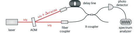
Figure 1: Experimental setup for the DSH beat note measurement. The laser beam is separated by an AOM, where one arm of the signal is frequency shifted and delayed by a long fiber. Both beams are superimposed at a photodetector, which captures only the slow beat note signal.

In the DSH measurement method, see Fig. 1, the light of a laser is superimposed with the frequency-shifted (heterodyne) and time-delayed light from the same source. The frequency shift $\Delta\omega_{\mathrm{AOM}}$ (typically several tens of MHz) is realized with an acousto-optic modulator (AOM) and the delay $\tau_{d}$ is implemented via long fibers (typically several km). If the delay is larger than the coherence time of the laser, the delayed light can be regarded as a statistically independent second laser with the same frequency and noise characteristics. The DSH method allows to down-convert the optical signal to a beat note signal in the RF domain, that can be resolved by corresponding spectrum analyzers. Unlike other methods, the DSH method does not require stabilization of the laser to an optical reference (e.g., a frequency-stabilized second laser). Moreover, the frequency noise characteristics can be measured over a broad frequency bandwidth. A detailed description of the experimental setup and the post-processing procedure can be found in Ref. 31.

After down-conversion and $I$–$Q$ demodulation (Hilbert transform) is carried out by the spectrum analyzer, the detected in-phase and quadrature signals read [31]

$$I\left(t\right) =\eta_{\mathrm{det}}\sqrt{P\left(t\right)P\left(t-\tau_{d}\right)}\,\cos{\left(\phi\left(t\right)-\phi\left(t-\tau_{d}\right)-\Delta\Omega\,t\right)}+\xi_{I}\left(t\right),$$ (1a)

$$Q\left(t\right) =\eta_{\mathrm{det}}\sqrt{P\left(t\right)P\left(t-\tau_{d}\right)}\,\sin{\left(\phi\left(t\right)-\phi\left(t-\tau_{d}\right)-\Delta\Omega\,t\right)}+\xi_{Q}\left(t\right),$$ (1b)

where $\eta_{\mathrm{det}}$ is the detector efficiency, $P$ is the photon number, $\phi$ is the optical phase and $\Delta\Omega$ is the final difference frequency accumulated in the beating of the signal in the interferometer and the RF analyzer, where the sum frequency components are filtered out. We assume Gaussian white measurement noise with correlation function $\left\langle\xi_{I}\left(t\right)\xi_{I}\left(t^{\prime}\right)\right\rangle=\left\langle\xi_{Q}\left(t\right)\xi_{Q}\left(t^{\prime}\right)\right\rangle=\sigma_{\mathrm{meas}}^{2}\delta\left(t-t^{\prime}\right)$.

From the measured time series $I\left(t\right)$, $Q\left(t\right)$ one easily obtains the phase fluctuation difference

$$\Delta\phi\left(t\right)=\delta\phi\left(t\right)-\delta\phi\left(t-\tau_{d}\right)=\arctan\left(\frac{Q\left(t\right)}{I\left(t\right)}\right)-\overline{\Omega}\tau_{d}+\Delta\Omega\,t+\xi_{\phi}\left(t\right)$$ (2)

where $\overline{\Omega}$ is the nominal CW frequency and $\delta\phi(t)=\phi(t)-\overline{\Omega}t$. The effective measurement noise $\xi_{\phi}\left(t\right)$ (which derives from $\xi_{I}\left(t\right)$ and $\xi_{Q}\left(t\right)$) is approximately white

$$\left\langle\xi_{\phi}\left(t\right)\xi_{\phi}\left(t^{\prime}\right)\right\rangle\approx\left(\frac{\sigma_{\mathrm{meas}}}{\eta_{\mathrm{det}}\overline{P}}\right)^{2}\delta\left(t-t^{\prime}\right),$$ (3)

if the average power $\overline{P}$ is much larger than the measurement noise level $\sigma_{\mathrm{meas}}$, see Appendix A. The evaluation of Eq. (2) requires estimation of $\tau_{d}$ and $\Delta\Omega$ (detrending), see [31] for details.

In the frequency domain, the relation between the phase fluctuations $\delta\phi\left(t\right)$ and $\Delta\phi\left(t\right)$ reads

$$\Delta\tilde{\phi}\left(\omega\right)=H\left(\omega\right)\delta\tilde{\phi}\left(\omega\right),\qquad H\left(\omega\right)=1-\mathrm{e}^{i\omega\tau_{d}},$$ (4)

from which one derives a simple relation between the corresponding phase noise PSDs

$$S_{\Delta\phi,\Delta\phi}\left(\omega\right)=\left|H\left(\omega\right)\right|^{2}S_{\delta\phi,\delta\phi}\left(\omega\right).$$ (5)

In the standard post-processing routine [19, 31], Eq. (5) is solved for $S_{\delta\phi,\delta\phi}\left(\omega\right)$ by division through $\left|H\left(\omega\right)\right|^{2}=2\left(1-\cos{\left(\omega\tau_{d}\right)}\right)$. This approach has two notable shortcomings: First, this procedure does not take into account the detector noise and thereby fails at increased measurement noise levels. Second, the transfer function has roots at $\omega_{n}=2\pi n/\tau_{d}$, $n\in\mathbb{Z}$, which turn to poles in its inverse $\left|G\left(\omega\right)\right|^{2}=\left|H\left(\omega\right)\right|^{-2}$. Hence, the reconstructed PSD exhibits a series of equidistant spurious spikes [32, 33, 34], resulting from an uncontrolled amplification of the measurement noise.

III Parametric Wiener Filters

In this section, we present the Wiener deconvolution method for reconstructing hidden signals from noisy time series data. Besides the well-known Wiener filter, we introduce power spectrum equalization (PSE) as an important representative of the group of parametric Wiener filters [35].

Let $x\left(t\right)$ denote the time series of a hidden signal of interest that is measured by an experimental setup characterized by a convolution kernel $h\left(t\right)$. In the case of the DSH measurement described above, this is $h\left(t\right)=\delta\left(t\right)-\delta\left(t-\tau_{d}\right)$. Furthermore, let $\xi\left(t\right)$ denote additive Gaussian white measurement noise. Then the experiment yields an observed time series

$$z\left(t\right)=\left(h*x\right)\left(t\right)+\xi\left(t\right).$$ (6a)

The process noise and measurement noise are assumed to be uncorrelated $$\langle x\left(t\right)\xi\left(t^{\prime}\right)\rangle=0 \hat{x}\left(t\right)$$. One seeks for an optimal estimate of the hidden signal

$$\hat{x}\left(t\right)=\left(g*z\right)\left(t\right),$$ (6b)

where the (de-)convolution kernel $g\left(t\right)$ minimizes the reconstruction error.

In this paper, our main interest is the reconstruction of PSDs of hidden signals in the frequency domain, for which we introduce the Fourier space representation of Eq. (6)

$$Z\left(\omega\right) =H\left(\omega\right)X\left(\omega\right)+\Xi\left(\omega\right),$$ (7a)

$$\hat{X}\left(\omega\right) =G\left(\omega\right)Z\left(\omega\right).$$ (7b)

From Eq. (7b), we obtain the relation between the estimated PSD $S_{\hat{x},\hat{x}}\left(\omega\right)$ of the hidden signal and the PSD of the measured time series $S_{z,z}\left(\omega\right)$

$$S_{\hat{x},\hat{x}}\left(\omega\right)=\left|G\left(\omega\right)\right|^{2}S_{z,z}\left(\omega\right).$$ (8)

In the following, we discuss different candidates for the filter function $G\left(\omega\right)$. Their performance is assessed with regard to the reconstruction of the FN–PSD of a semiconductor laser [20, 22, 23] from DSH measurements. The transfer function of the interferometer is

$$H\left(\omega\right)=1-\mathrm{e}^{i\omega\tau_{d}}$$

and we assume the hidden signal and noise PSDs as

$$S_{x,x}\left(\omega\right) =\frac{C}{\omega^{\nu}}+S_{\infty},$$ (9)

$$S_{\xi,\xi}\left(\omega\right) =\sigma\omega^{2}.$$ (10)

In Eq. (9), $S_{\infty}$ determines the intrinsic laser linewidth, which is obscured by additional colored noise of power-law type with $0.8\lesssim\nu\lesssim 1.6$ (flicker noise). The functional form of Eq. (9) is consistent with theoretical models and experimental observations for frequencies well below the relaxation oscillation (RO) peak (typically at several GHz). The level of phase measurement noise, cf. Eq. (3), is specified by $\sigma$ and the corresponding frequency measurement noise PSD is a quadratic function of the frequency. The model PSDs (9)–(10) imply the signal-to-noise ratio

$$\mathrm{SNR}\left(\omega\right)=S_{x,x}\left(\omega\right)/S_{\xi,\xi}\left(\omega\right).$$ (11)

Figure 2 shows that different filters $G\left(\omega\right)$ can lead to vastly different results for $S_{\hat{x},\hat{x}}\left(\omega\right)$. In the following section, we discuss their behavior in more detail.

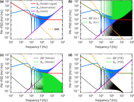
Figure 2: Comparison of different filters $G\left(\omega\right)$ for FN–PSD reconstruction. (a) Analytical signal Eq. (9) and measurement noise PSD (10) along with the observed spectrum and the exact SNR. Parameters in the plot are $\nu=1.4$, $C=10^{11}\,\mathrm{Hz}^{\nu+1}$, $S_{\infty}=10^{3}\,\mathrm{Hz}$, $\sigma=10^{-10}\,\mathrm{Hz}$ and $\tau_{d}=10$ µ$\mathrm{s}$. (b) The inverse filter Eq. (12) yields a reconstructed PSD with spurious peaks at the pole frequencies $f_{n}=n/\tau_{d}$, $n\in\mathbb{Z}$. The intrinsic linewidth plateau is obscured by detector noise and can not be recovered from the inverse filter (merely an upper limit can be extracted). (c) The Wiener filter Eq. (13) is optimized for time series reconstruction, but fails in reconstruction of the PSD. The reconstructed PSD features sharp dropouts at the pole frequencies and does not follow the hidden signal at low $\mathrm{SNR}<1$. (d) Power spectrum equalization Eq. (14) yields an exact reconstruction of the hidden signal’s PSD if the exact SNR is provided. Here, the singularities at the pole frequencies are bounded from above by the SNR, which allows for exact compensation of both the detector noise and the interferometer effects in the observed signal $S_{z,z}$.

III.1 Inverse Filter

In the case of negligible detector noise, the filter $G\left(\omega\right)$ is given by the inverse transfer function

$$G_{\mathrm{inv}}\left(\omega\right)=H^{-1}\left(\omega\right).$$ (12)

The corresponding estimate of the PSD of the hidden signal reads

$$S_{\hat{x},\hat{x}}\left(\omega\right) =\left|G_{\mathrm{inv}}\left(\omega\right)\right|^{2}S_{z,z}\left(\omega\right), \left|G_{\mathrm{inv}}\left(\omega\right)\right|^{2} =\left|H\left(\omega\right)\right|^{-2},$$

which coincides with the standard post-processing method of the DSH measurement [19, 29, 33], cf. Eq. (5). The most prominent feature of the inverse filter $\left|G_{\mathrm{inv}}\left(\omega\right)\right|^{2}$ are singularities at the poles $\omega_{n}^{\mathrm{pole}}=2\pi n/\tau_{d}$, $n\in\mathbb{Z}$, where the PSD reconstruction fails, see Fig. 2 (b). Sufficiently far away from these poles, the reconstructed spectrum matches the hidden signal as long as the signal-to-noise ratio is large ($\mathrm{SNR}>1$). If the intrinsic linewidth plateau is obscured by measurement noise, only an upper limit can be extracted via inverse filtering.

III.2 Wiener Filter

Wiener filtering achieves an optimal trade-off between inverse filtering and noise removal. It subtracts the additive noise and reverses the effects of the interferometer simultaneously. The Wiener filter is obtained from minimizing the mean square error of the time-domain signal at an arbitrary instance of time, see Appendix B.1. In the frequency domain, the Wiener filter reads

$$\begin{aligned} G_{\mathrm{Wiener}}\left(\omega\right)&=\frac{H^{*}\left(\omega\right)S_{x,x}\left(\omega\right)}{\left|H\left(\omega\right)\right|^{2}S_{x,x}\left(\omega\right)+S_{\xi,\xi}\left(\omega\right)}\\ &=\frac{1}{H\left(\omega\right)}\left(1+\frac{1}{\left|H\left(\omega\right)\right|^{2}\mathrm{SNR}\left(\omega\right)}\right)^{-1}.\end{aligned}$$ (13)

Although the Wiener filter provides an optimal reconstruction of the time-domain signal, the corresponding PSD reconstruction deviates significantly from the true spectrum in regions of low SNR, see Fig. 2 (c). Moreover, we note that the Wiener filter overemphasizes noise reduction at the poles $\omega_{n}^{\mathrm{pole}}$, where the reconstructed PSD is zero because of $\big{|}G_{\mathrm{Wiener}}\big{(}\omega_{n}^{\mathrm{pole}}\big{)}\big{|}^{2}=0$, such that also $S_{\hat{x},\hat{x}}\big{(}\omega_{n}^{\mathrm{pole}}\big{)}=0$. Away from these poles and at high SNR, the Wiener filter asymptotically approaches the behavior of the inverse filter: $\big{|}G_{\mathrm{Wiener}}\big{(}\omega\neq\omega_{n}^{\mathrm{pole}}\big{)}\big{|}^{2}\stackrel{{\scriptstyle\mathrm{SNR}\to\infty}}{{\sim}}\left|H\left(\omega\right)\right|^{-2}$.

III.3 Power Spectrum Equalization

Besides the standard Wiener filter, there exist several variants of the method which are collectively referred to as parametric Wiener filters [35]. An important one is power spectrum equalization (PSE), which is tailored to minimize the quadratic error of the reconstructed PSD, see Appendix B.2. The corresponding filter function reads

$$\begin{aligned} \bigl{|}G_{\mathrm{PSE}}\left(\omega\right)\bigr{|}^{2}&=\frac{S_{x,x}\left(\omega\right)}{\left|H\left(\omega\right)\right|^{2}S_{x,x}\left(\omega\right)+S_{\xi,\xi}\left(\omega\right)}\\ &=\frac{1}{\left|H\left(\omega\right)\right|^{2}}\left(1+\frac{1}{\left|H\left(\omega\right)\right|^{2}\mathrm{SNR}\left(\omega\right)}\right)^{-1}.\end{aligned}$$ (14)

The PSE filter yields an accurate reconstruction of the hidden signal when the true frequency-dependent SNR is provided, see Fig. 2 (d).

Most remarkably, the reconstructed spectrum is free of reconstruction artifacts at the poles of the inverse filter function. This result is easily understood by the following analysis. A straightforward calculation shows that the filter approaches the SNR at $\omega_{n}^{\mathrm{pole}}$: $\big{|}G_{\mathrm{PSE}}\big{(}\omega_{n}^{\mathrm{pole}}\big{)}\big{|}^{2}=\mathrm{SNR}\big{(}\omega_{n}^{\mathrm{pole}}\big{)}$. As the interferometer is blind for these frequency components (i.e., the transfer function is zero $H\big{(}\omega_{n}^{\mathrm{pole}}\big{)}=0$), the observed signal contains only measurement noise $S_{z,z}\big{(}\omega_{n}^{\mathrm{pole}}\big{)}=S_{\xi,\xi}\big{(}\omega_{n}^{\mathrm{pole}}\big{)}$, see Eq. (7b). Finally, substitution into Eq. (8), shows that the PSE filter cancels out the measurement noise exactly and recovers the true signal

$$S_{\hat{x},\hat{x}}\big{(}\omega_{n}^{\mathrm{pole}}\big{)}=\bigl{|}G_{\mathrm{PSE}}\big{(}\omega_{n}^{\mathrm{pole}}\big{)}\bigr{|}^{2}\,S_{z,z}\big{(}\omega_{n}^{\mathrm{pole}}\big{)}=\mathrm{SNR}\big{(}\omega_{n}^{\mathrm{pole}}\big{)}\,S_{\xi,\xi}\big{(}\omega_{n}^{\mathrm{pole}}\big{)}=S_{x,x}\big{(}\omega_{n}^{\mathrm{pole}}\big{)}$$

if the correct SNR is provided. Furthermore, we observe that the PSE filter restores the hidden signal even in regions of low SNR. This result follows along the same lines as above, starting from $\bigl{|}G_{\mathrm{PSE}}\left(\omega\right)\bigr{|}^{2}\stackrel{{\scriptstyle\mathrm{SNR}\to 0}}{{\sim}}\mathrm{SNR}\left(\omega\right)$. In the opposite case, at very high $\mathrm{SNR}\left(\omega\right)\gg 1$, the PSE filter again approaches (just like the Wiener filter) the inverse filter $\bigl{|}G_{\mathrm{PSE}}\left(\omega\right)\bigr{|}^{2}\stackrel{{\scriptstyle\mathrm{SNR}\to\infty}}{{\sim}}\left|H\left(\omega\right)\right|^{-2}.$

Finally, we note that all the filter candidates discussed in this section can be written in a unified way as parametric Wiener filters of the following form:

$$\bigl{|}G\left(\omega\right)\bigr{|}^{2}=\frac{1}{\left|H\left(\omega\right)\right|^{2}}\left(1+\frac{1}{\left|H\left(\omega\right)\right|^{2}\mathrm{SNR}\left(\omega\right)}\right)^{-m}=\begin{cases}\bigl{|}G_{\mathrm{inv}}\left(\omega\right)\bigr{|}^{2}&\text{for }m=0,\\ \bigl{|}G_{\mathrm{Wiener}}\left(\omega\right)\bigr{|}^{2}&\text{for }m=1,\\ \bigl{|}G_{\mathrm{PSE}}\left(\omega\right)\bigr{|}^{2}&\text{for }m=2.\end{cases}$$

IV Intrinsic Linewidth Estimation at Low Signal-to-Noise Ratio

In the previous section, it was shown that the PSE filter can provide an excellent reconstruction of the hidden signal’s PSD if the exact SNR is supplied. At first glance, this approach appears to be rather impractical, since the specification of the exact SNR already anticipates the actual measurement result to a certain degree. One might therefore worry that arbitrary reconstructions could be generated. It turns out, however, that the PSE filter method introduces characteristic reconstruction artifacts when the specified SNR is incorrect, see Fig. 3. These spurious spikes are easily recognized to be unphysical, such that the incorrect SNR estimate can be rejected. Based on this observation, we develop a method that simultaneously reconstructs both the PSD of the hidden signal as well as the correct SNR, by minimizing these reconstruction artifacts.

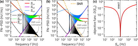
Figure 3: Reconstruction artifacts in the PSE filter method with incorrectly estimated SNR. (a) Overestimation ($S_{\infty}^{\mathrm{est}}=5S_{\infty}$) and (b) underestimation ($S_{\infty}^{\mathrm{est}}=0.2S_{\infty}$) of the intrinsic linewidth $S_{\infty}$ leads to spurious oscillations and spikes in the reconstructed spectrum $S_{\hat{x},\hat{x}}$. In the case of misspecification of the SNR, the maxima of $\left|G_{\mathrm{PSE}}\right|^{2}$ are no longer bounded by the exact SNR. The assumed $\overline{S}_{x,x}$, which has the functional form (9) and enters the SNR estimate, is shown as a red dashed line. The method described in Sec. IV aims at minimizing the deviation between $\overline{S}_{x,x}$ and $S_{\hat{x},\hat{x}}$ in order to estimate the true value of the intrinsic linewidth parameter $S_{\infty}$. (c) The corresponding objective function (15) features a sharp minimum at the exact value.

In the following, we employ again the analytic model PSDs (9)–(10). For the sake of simplicity, we assume that the parameters $C$ and $\nu$ can be accurately estimated from the data, since the low-frequency part of the signal is only negligibly affected by measurement noise. Similarly, we assume that the noise level $\sigma$ is known from independent noise floor measurements or from analysis of the relative intensity noise (RIN) PSD, which is typically dominated by measurement noise at increased powers. The only free parameter to be estimated then is $S_{\infty}$.

Figure 3 (a)–(b) shows the effects of over- and underestimation of $S_{\infty}$ in the analytical model. Due to the mismatch between the filter function $\left|G_{\mathrm{PSE}}\left(\omega\right)\right|^{2}$ and the observed spectrum $S_{z,z}\left(\omega\right)$, spurious spikes (reconstruction artifacts) show up at frequencies $\omega\approx\omega_{n}^{\mathrm{pole}}$ in the reconstructed spectrum $S_{\hat{x},\hat{x}}\left(\omega\right)$. At large frequencies these spikes are damped out in both $\left|G_{\mathrm{PSE}}\left(\omega\right)\right|^{2}$ and $S_{z,z}\left(\omega\right)$, but their product yields a wrong value of the intrinsic linewidth plateau. We introduce an objective function $D\left(S_{\infty}\right)$ that penalizes this deviation (i.e., the “inconsistency”) between the reconstructed signal $S_{\hat{x},\hat{x}}\left(\omega;S_{\infty}\right)$ (depending on the assumed SNR as a function of estimated $S_{\infty}$) and the implicitly assumed signal $\overline{S}_{x,x}\left(\omega;S_{\infty}\right)$ obeying the functional form (9) as

$$D\left(S_{\infty}\right)=\left(\int\mathrm{d}\omega\,\frac{S_{\hat{x},\hat{x}}\left(\omega;S_{\infty}\right)-\overline{S}_{x,x}\left(\omega;S_{\infty}\right)}{\overline{S}_{x,x}\left(\omega;S_{\infty}\right)}\right)^{2}$$ (15)

where $S_{\hat{x},\hat{x}}\left(\omega;S_{\infty}\right)=\left|G_{\mathrm{PSE}}\left(\omega;S_{\infty}\right)\right|^{2}S_{z,z}\left(\omega\right)$. The $\omega$–integral runs over a suitable frequency range. As shown in Fig. 3 (c), the objective function (15) exhibits a sharp minimum at the exact value, cf. Fig. 2 (c). Hence, $S_{\infty}$ can be estimated by minimization of $D(S_{\infty})$.

V Application to Stochastic Laser Dynamics

In this section, we demonstrate the method described in Sec. IV for simulated time series. In Sec. V.1, we introduce a stochastic laser model including non-Markovian colored noise, that generates realistic time series with frequency drifts as commonly observed for diode lasers. In Sec. V.2, we apply the linewidth estimation method to simulated DSH measurement data.

V.1 Stochastic Laser Rate Equations

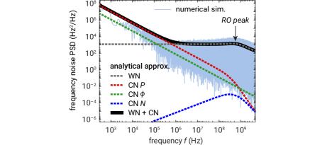
Figure 4: Numerically computed FN–PSD from simulated time series using the stochastic laser rate Eqs. (16). Analytical approximations are derived from linearization of the model at the noise-free steady state. White noise (WN) and different colored noise (CN) contributions are indicated separately.

We consider a Langevin equation model for a generic single-mode semiconductor laser

$$\dot{P} =-\gamma\left(P-P_{\mathrm{th}}\right)+\Gamma v_{g}g\left(P,N\right)P+\Gamma v_{g}g_{\mathrm{sp}}\left(P,N\right)+F_{P},$$ (16a)

$$\dot{\phi} =\Omega_{0}+\frac{\alpha_{H}}{2}\Gamma v_{g}g\left(P,N\right)+F_{\phi},$$ (16b)

$$\dot{N} =\frac{\eta I}{q}-R\left(N\right)-\Gamma v_{g}g\left(P,N\right)P-\Gamma v_{g}g_{\mathrm{sp}}\left(P,N\right)+F_{N},$$ (16c)

where $P$ is the number of photons, $\phi$ is the optical phase and $N$ is the number of charge carriers in the active region. Moreover, $\gamma$ is the inverse photon lifetime, $P_{\mathrm{th}}$ is the thermal photon number (Bose–Einstein factor), $\Gamma$ is the optical confinement factor, $v_{g}$ is the group velocity, $\Omega_{0}$ is the detuning from the CW reference frequency, $\alpha_{H}$ is the linewidth enhancement factor, $I$ is the pump current, $\eta$ is the injection efficiency and $q$ is the elementary charge. The net-gain is modeled as

$$g\left(P,N\right)=\frac{g_{0}}{1+\varepsilon P}\log{\left(\frac{N}{N_{\mathrm{tr}}}\right)},$$ (17)

where $g_{0}$ is the gain coefficient, $N_{\mathrm{tr}}$ is the carrier number at transparency and $\varepsilon$ is the gain compression coefficient. Following [18], the spontaneous emission coefficient is described by

$$g_{\mathrm{sp}}\left(P,N\right)=\frac{1}{2}\frac{g_{0}}{1+\varepsilon P}\log{\left(1+\left(\frac{N}{N_{\mathrm{tr}}}\right)^{2}\right)},$$ (18)

which does not require any additional parameters and avoids the introduction of the population inversion factor [17, 18]. The stimulated absorption coefficient is implicitly given by Eqs. (17)–(18) as $g_{\mathrm{abs}}\left(P,N\right)=g_{\mathrm{sp}}\left(P,N\right)-g\left(P,N\right)$. Non-radiative recombination and spontaneous emission into waste modes are described by

$$R\left(N\right)=AN+\frac{B}{V}N^{2}+\frac{C}{V^{2}}N^{3},$$ (19)

where $A$ is the Shockley–Read–Hall recombination rate, $B$ is the bimolecular recombination coefficient, $C$ is the Auger recombination coefficient and $V$ is the volume of the active region.

symbol	description	value
$\gamma$	inverse photon lifetime	$5\cdot 10^{11}\,\mathrm{s}^{-1}$
$P_{\mathrm{th}}$	thermal photon number	$2.7\cdot 10^{-20}$
$\Gamma$	optical confinement factor	$0.01$
$g_{0}$	gain coefficient	$3.54\cdot 10^{5}\,\mathrm{m}^{-1}$
$n_{g}$	group index	$3.9$
$v_{g}$	group velocity, $v_{g}=n_{g}/c_{0}$	$7.69\cdot 10^{7}\,\mathrm{m}\mathrm{s}^{-1}$
$N_{\mathrm{tr}}$	transparency carrier number	$2.5\cdot 10^{9}$
$\varepsilon$	gain compression coefficient	$10^{-8}$
$\Omega_{0}$	detuning from CW reference freq.	$0\,\mathrm{Hz}$
$\alpha_{H}$	linewidth enhancement factor	$3.0$
$I$	pump current	$200\,\mathrm{mA}$
$\eta$	injection efficiency	$0.9$
$A$	Shockley–Read–Hall recombination rate	$1\cdot 10^{8}\,\mathrm{s}^{-1}$
$B$	bimolecular recombination coefficient	$1\cdot 10^{16}\,\mathrm{m}^{3}\mathrm{s}^{-1}$
$C$	Auger recombination coefficient	$4\cdot 10^{-42}\,\mathrm{m}^{6}\mathrm{s}^{-1}$
$V$	active region volume	$1.25\cdot 10^{-15}\,\mathrm{m}^{3}$
$\nu_{P}$	colored noise exponent	$1.4$
$\sigma_{P,0}$	colored noise amplitude	$5\cdot 10^{5}\,\mathrm{s}^{-(1+\nu_{P})/2}$
$\nu_{N}$	colored noise exponent	$1.0$
$\sigma_{N,0}$	colored noise amplitude	$10^{9}\,\mathrm{s}^{-(1+\nu_{N})/2}$
$\sigma_{\mathrm{meas}}$	detector noise floor level	$2\cdot 10^{3}\,\mathrm{s}^{1/2}\,\eta_{\mathrm{det}}$
$\tau_{d}$	interferometer delay	$10\cdot 10^{-6}\,\mathrm{s}$

Table 1: List of parameter values used in stochastic time series simulation.

The Langevin forces describe zero-mean Gaussian colored noise with the following non-vanishing frequency-domain correlation functions:

$$\begin{aligned} \langle\tilde{F}_{P}\left(\omega\right)\tilde{F}_{P}\left(\omega^{\prime}\right)\rangle&=\left(2\left(\Gamma v_{g}g_{\mathrm{sp}}\big{(}\overline{P},\overline{N}\big{)}+\gamma P_{\mathrm{th}}\right)\overline{P}\left(1+\frac{1}{\overline{P}}\right)+\sigma_{P}^{2}\big{(}\overline{P}\big{)}\frac{1}{\omega^{\nu_{P}}}\right)\,\delta\left(\omega-\omega^{\prime}\right),\\ \langle\tilde{F}_{\phi}\left(\omega\right)\tilde{F}_{\phi}\left(\omega^{\prime}\right)\rangle&=\left(\left(\Gamma v_{g}g_{\mathrm{sp}}\big{(}\overline{P},\overline{N}\big{)}+\gamma P_{\mathrm{th}}\right)\left(1+\frac{1}{\overline{P}}\right)+\left(\frac{\sigma_{P}\big{(}\overline{P}\big{)}}{2\overline{P}}\right)^{2}\frac{1}{\omega^{\nu_{P}}}\right)\,\delta\left(\omega-\omega^{\prime}\right),\\ \langle\tilde{F}_{N}\left(\omega\right)\tilde{F}_{N}\left(\omega^{\prime}\right)\rangle&=\left(2R\big{(}\overline{N}\big{)}+2\Gamma v_{g}g_{\mathrm{sp}}\big{(}\overline{P},\overline{N}\big{)}\overline{P}\left(1+\frac{1}{\overline{P}}\right)+\frac{\sigma_{N}^{2}\big{(}\overline{N}\big{)}}{\omega^{\nu_{N}}}\right)\,\delta\left(\omega-\omega^{\prime}\right),\\ \langle\tilde{F}_{P}\left(\omega\right)\tilde{F}_{N}\left(\omega^{\prime}\right)\rangle&=-\left(\Gamma v_{g}g_{\mathrm{sp}}\big{(}\overline{P},\overline{N}\big{)}\left(2\overline{P}+1\right)-\Gamma v_{g}g\big{(}\overline{P},\overline{N}\big{)}\overline{P}\right)\,\delta\left(\omega-\omega^{\prime}\right),\end{aligned}$$ (20)

The white noise part of the model includes a quantum mechanically consistent description of light-matter interaction fluctuations [36]. Moreover, we have included three independent $1/f$-type noise sources with power-law exponents $\nu_{P}$ and $\nu_{N}$, respectively. The colored noise amplitudes are taken as $\sigma_{P}\left(P\right)=2P\sigma_{P,0}$ and $\sigma_{N}\left(N\right)=\sqrt{N}\sigma_{N,0}$ (modeling Hooge’s law [37, 38]). The noise correlation functions (20) are formulated at the unique noise-free steady state $\big{(}\overline{P},\overline{N}\big{)}$. The full nonlinear system of Itô-type stochastic differential equations used for simulation is given in Appendix C. The numerically simulated FN–PSD is shown in Fig. 4 along with (semi-)analytical approximations. All parameter values used in the simulations are listed in Tab. 1.

V.2 Intrinsic Linewidth Estimation

We apply the method described in Sec. IV to simulated DSH measurements. The simulation is carried out in two steps: First, the stochastic laser rate Eqs. (16) are simulated using the Euler–Maruyama method (time step $\Delta t=50\,\mathrm{ps}$). In the second step, the DSH measurement is simulated by evaluation of Eq. (1), which includes addition of Gaussian white measurement noise. The simulated $I$–$Q$ data are used to generate the time series $\Delta\phi$ according to Eq. (2). The observed spectrum is computed from $S_{z,z}\left(\omega\right)=\omega^{2}S_{\Delta\phi,\Delta\phi}\left(\omega\right)$ and shown in Fig. 5 (a). For recovery of the original FN–PSD, the PSE filter method is applied to the simulated FN–PSD $S_{z,z}\left(\omega\right)$. In the estimation procedure, the frequency range is restricted to frequencies below the RO peak to ensure validity of the analytical model (9).

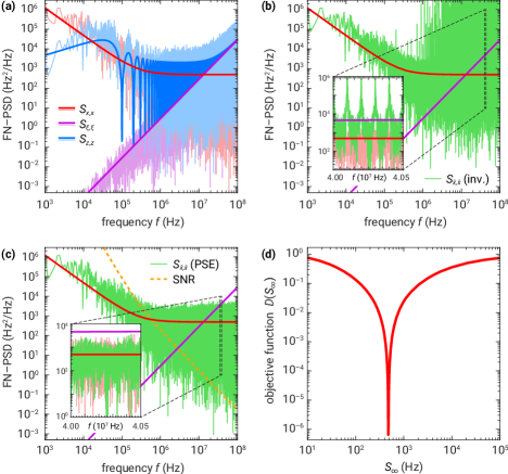
Figure 5: Application of the linewidth estimation method to simulated time series data. (a) PSDs of the hidden signal, the measurement noise and the measured data along with their analytic values. (b) Reconstructed PSD using the inverse filter. The inset zooms in on a region with low SNR, where the reconstructed and the true signal deviate by about one order of magnitude. Moreover, we observe reconstruction artifacts at the pole frequencies. (c) The PSE filter method yields an accurate reconstruction of the hidden signal even at low SNR that is free of reconstruction artifacts. Here the analytic model PSDs were fitted to the PSD to give the SNR according to the method described in Sec. IV. (d) Minimization of the objective function (15) yields a sharp estimate of the intrinsic linewidth parameter at $S_{\infty}\approx 480\,\mathrm{Hz}$.

The optimal reconstruction of the hidden FN–PSD is shown in Fig. 5 (c) along with corresponding SNR estimate and the measurement noise PSD. The PSE filter yields a significantly better reconstruction than the inverse filter method, which contains the characteristic reconstruction artifacts and deviates clearly from the hidden signal at increased measurement noise, see Fig. 5 (b). The objective function (15) evaluated for the simulated stochastic data is shown in Fig. 5 (d). Just like in Sec. IV, the objective function features a sharp minimum near at the exact value.

VI Discussion

The method presented in Sec. IV not only provides an artifact-free reconstruction of the hidden FN–PSD, but also allows to extract the intrinsic linewidth when it is obscured by measurement noise. The procedure, however, relies on the specification of the frequency-dependent SNR in the form of the analytical model (9)–(10). As we have demonstrated in Fig. 3, incorrect SNR estimates lead to reconstruction errors, which are identified as such via inconsistencies with the assumed functional form (9) of the hidden PSD. This a priori assumption of the functional, however, is well validated [20, 22, 23], so that no false bias is imposed here. Instead, our method exploits this additional prior knowledge about the physics of the problem to extract additional information (weak modulations of the measured PSD) from the measured data that is not used in the inverse filter method.

Even though we restricted the parameter estimation problem in Secs. IV and V.2 to a single unknown variable, it should be straightforward to extend the method to a multivariate (nonlinear) minimization problem where all parameters characterizing the SNR are estimated simultaneously. Furthermore, it would be interesting to apply the estimation method in an analogous way to the reconstruction of the RIN, which is typically more obscured by detector noise.

In principle other estimation methods can also be employed for reconstruction of the FN–PSD from noisy time series data. For example, Zibar et al. [39] have used an extended Kalman filter to estimate the effect of amplifier noise on the phase noise PSD of a laser. The disadvantage of this method, however, is that it requires a (comprehensive) mathematical model of the dynamical system under measurement, which imposes a significant overhead. Moreover, the application of Kalman filters to problems with large delay (like the DSH-measurement), is notoriously difficult and computationally heavy [40, 41]. In contrast, the strength of parametric Wiener filters is that they are independent of assumptions on the underlying state space model. Moreover, since the method is formulated in the frequency-domain, it does not suffer from computational burden due to the large delay. Finally, the method is simple to implement, as it is basically a straightforward extension of the standard inverse filter method (that is still contained as a limiting case).

VII Summary

We have presented an improved post-processing routine based on a parametric Wiener filter, that yields a potentially exact reconstruction of the FN–PSD (without any reconstruction artifacts) from DSH beat note measurements. The method, however, requires an accurate estimate of the frequency-dependent SNR, which can be consistently obtained by deliberate suppression of the characteristic reconstruction artifacts. In this way, both the footprint of the interferometer as well as the detector noise can be removed with high accuracy. Remarkably, the method thus allows for the reconstruction of the intrinsic linewidth (white noise) plateau even when it is entirely obscured by measurement noise. The approach has been demonstrated for simulated time series based on a stochastic laser rate equation model including non-Markovian $1/f$-type noise.

Appendix

Appendix A Effective Phase Measurement Noise

We seek for an approximation of the effective phase measurement noise and its two-time correlation function. Starting from Eq. (1), we expand for small noise

$$\arctan\left(\frac{Q\left(t\right)}{I\left(t\right)}\right)\approx\arctan\left(\tan{\left(\Phi(t)\right)}+\frac{\tan{\left(\Phi\left(t\right)\right)}}{\eta_{\mathrm{det}}\sqrt{P\left(t\right)P\left(t-\tau_{d}\right)}}\left(\frac{\xi_{Q}\left(t\right)}{\sin{\left(\Phi(t)\right)}}-\frac{\xi_{I}\left(t\right)}{\cos{\left(\Phi(t)\right)}}\right)\right)$$

where $\Phi\left(t\right)=\phi\left(t\right)-\phi\left(t-\tau_{d}\right)-\Delta\Omega\,t$. Expansion to first order yields

$$\arctan\left(\frac{Q\left(t\right)}{I\left(t\right)}\right)\approx\Phi\left(t\right)+\frac{1}{\eta_{\mathrm{det}}\sqrt{P\left(t\right)P\left(t-\tau_{d}\right)}}\left(\cos{\left(\Phi\left(t\right)\right)}\xi_{Q}\left(t\right)-\sin{\left(\Phi\left(t\right)\right)}\xi_{I}\left(t\right)\right).$$

Expansion at the CW state with $P\left(t\right)=\overline{P}+\delta P\left(t\right)$ and $\phi\left(t\right)=\overline{\Omega}t+\delta\phi\left(t\right)$ yields

$$\Delta\phi\left(t\right)=\delta\phi\left(t\right)-\delta\phi\left(t-\tau_{d}\right)\approx\arctan\left(\frac{Q\left(t\right)}{I\left(t\right)}\right)-\overline{\Omega}\tau_{d}+\Delta\Omega\,t+\xi_{\phi}$$

with the effective phase measurement noise

$$\xi_{\phi}\left(t\right)=\frac{1}{\eta_{\mathrm{det}}\sqrt{P\left(t\right)P\left(t-\tau_{d}\right)}}\left(\sin{\left(\Phi\left(t\right)\right)}\xi_{I}\left(t\right)-\cos{\left(\Phi\left(t\right)\right)}\xi_{Q}\left(t\right)\right).$$

We approximate the two-time correlation function

$$\left\langle\xi_{\phi}\left(t\right)\xi_{\phi}\left(t^{\prime}\right)\right\rangle \approx\frac{1}{\eta_{\mathrm{det}}^{2}\overline{P}^{2}}\Big{(}\left\langle\sin{\left(\Phi\left(t\right)\right)}\sin{\left(\Phi\left(t^{\prime}\right)\right)}\right\rangle\left\langle\xi_{I}\left(t\right)\xi_{I}\left(t^{\prime}\right)\right\rangle$$

$$\hphantom{=\frac{1}{\eta_{\mathrm{det}}^{2}\overline{P}^{2}}\Big{(}}-\left\langle\cos{\left(\Phi\left(t\right)\right)}\sin{\left(\Phi\left(t^{\prime}\right)\right)}\right\rangle\left\langle\xi_{Q}\left(t\right)\xi_{I}\left(t^{\prime}\right)\right\rangle$$

$$\hphantom{=\frac{1}{\eta_{\mathrm{det}}^{2}\overline{P}^{2}}\Big{(}}-\left\langle\sin{\left(\Phi\left(t\right)\right)}\cos{\left(\Phi\left(t^{\prime}\right)\right)}\right\rangle\left\langle\xi_{I}\left(t\right)\xi_{Q}\left(t^{\prime}\right)\right\rangle$$

$$\hphantom{=\frac{1}{\eta_{\mathrm{det}}^{2}\overline{P}^{2}}\Big{(}}+\left\langle\cos{\left(\Phi\left(t\right)\right)}\cos{\left(\Phi\left(t^{\prime}\right)\right)}\right\rangle\left\langle\xi_{Q}\left(t\right)\xi_{Q}\left(t^{\prime}\right)\right\rangle\Big{)},$$

where we have neglected photon number fluctuations and factorized the phase and detector noise. Using $\left\langle\xi_{I}\left(t\right)\xi_{I}\left(t^{\prime}\right)\right\rangle=\left\langle\xi_{Q}\left(t\right)\xi_{Q}\left(t^{\prime}\right)\right\rangle=\sigma_{\mathrm{meas}}^{2}\delta\left(t-t^{\prime}\right)$ and stationarity $\left\langle\xi_{I}\left(t\right)\xi_{Q}\left(t^{\prime}\right)\right\rangle=\left\langle\xi_{I}\left(t^{\prime}\right)\xi_{Q}\left(t\right)\right\rangle$, we arrive at

$$\left\langle\xi_{\phi}\left(t\right)\xi_{\phi}\left(t^{\prime}\right)\right\rangle\approx\frac{1}{\eta_{\mathrm{det}}^{2}\overline{P}^{2}}\left(\sigma_{\mathrm{meas}}^{2}\delta\left(t-t^{\prime}\right)-\left\langle\sin{\left(\Phi\left(t\right)+\Phi\left(t^{\prime}\right)\right)}\right\rangle\left\langle\xi_{I}\left(t^{\prime}\right)\xi_{Q}\left(t\right)\right\rangle\right).$$

By neglecting the rapidly oscillating cross-correlation term, we arrive at Eq. (3).

Appendix B Derivation of the Frequency Domain Filter Functions

B.1 Wiener Filter

We consider the mean square error between the hidden signal $x\left(t\right)$ and its reconstruction Eq. (6b)

$$E\left(t\right)=\left\langle\left(\hat{x}\left(t\right)-x\left(t\right)\right)^{2}\right\rangle.$$

Fourier transform and substitution of (7) yields

$$E\left(t\right) =\int_{-\infty}^{\infty}\frac{\mathrm{d}\omega}{2\pi}\,\int_{-\infty}^{\infty}\frac{\mathrm{d}\omega^{\prime}}{2\pi}\,\mathrm{e}^{-i\left(\omega-\omega^{\prime}\right)t}\,\bigg{(}\left[G^{*}(\omega^{\prime})H^{*}(\omega^{\prime})-1\right]\left[G(\omega)H(\omega)-1\right]\left\langle X(\omega)X^{*}(\omega^{\prime})\right\rangle$$

$$\phantom{=}+2\mathrm{Re}\left(G^{*}\left(\omega^{\prime}\right)\left[G\left(\omega\right)H\left(\omega\right)-1\right]\left\langle X\left(\omega\right)\Xi^{*}\left(\omega^{\prime}\right)\right\rangle\right)+G^{*}\left(\omega^{\prime}\right)G\left(\omega\right)\left\langle\Xi\left(\omega\right)\Xi^{*}\left(\omega^{\prime}\right)\right\rangle\bigg{)}.$$

Next, we substitute the expressions for the signal and noise PSDs

$$\frac{1}{2\pi}\left\langle X\left(\omega\right)X^{*}\left(\omega^{\prime}\right)\right\rangle =S_{x,x}\left(\omega\right)\delta\left(\omega-\omega^{\prime}\right), \frac{1}{2\pi}\left\langle\Xi\left(\omega\right)\Xi^{*}\left(\omega^{\prime}\right)\right\rangle =S_{\xi,\xi}\left(\omega\right)\delta\left(\omega-\omega^{\prime}\right),$$

and assume uncorrelated process and measurement noise $\left\langle X\left(\omega\right)\Xi^{*}\left(\omega^{\prime}\right)\right\rangle=0$. This yields

$$E\left(t\right) =\int_{-\infty}^{\infty}\frac{\mathrm{d}\omega}{2\pi}\,\left(\left|G\left(\omega\right)H\left(\omega\right)-1\right|^{2}S_{x,x}\left(\omega\right)+\left|G\left(\omega\right)\right|^{2}S_{\xi,\xi}\left(\omega\right)\right),$$

which is entirely independent of the time $t$. Minimization of the reconstruction error $E\left(t\right)$ is achieved by taking the Gâteaux derivative with respect to $G\left(\omega\right)\to G\left(\omega\right)+\varepsilon\delta G\left(\omega\right)$

$$0\stackrel{{\scriptstyle!}}{{=}}\lim_{\varepsilon\to 0}\frac{E\left[G+\varepsilon\delta G\right]-E\left[G\right]}{\varepsilon} =\int_{-\infty}^{\infty}\frac{\mathrm{d}\omega}{2\pi}\,\Big{(}\left(G\left(\omega\right)H\left(\omega\right)-1\right)H^{*}\left(\omega\right)S_{x,x}\left(\omega\right)$$

$$\hphantom{=\int_{-\infty}^{\infty}\frac{\mathrm{d}\omega}{2\pi}\,\bigg{(}}+G\left(\omega\right)S_{\xi,\xi}\left(\omega\right)\Big{)}\delta G^{*}\left(\omega\right)+\mathrm{c.c.}$$

where the variation $\delta G\left(\omega\right)$ is arbitrary. From this, finally, we extract the Wiener filter Eq. (13).

B.2 Power Spectrum Equalization

We seek for an optimal reconstruction $S_{\hat{x},\hat{x}}\left(\omega\right)$ of the PSD that minimizes the quadratic error

$$E=\int_{-\infty}^{\infty}\mathrm{d}\omega\,\left(S_{\hat{x},\hat{x}}\left(\omega\right)-S_{x,x}\left(\omega\right)\right)^{2}.$$

Starting from $\langle\hat{X}\left(\omega\right)\hat{X}^{*}\left(\omega^{\prime}\right)\rangle=2\pi S_{\hat{x},\hat{x}}\left(\omega\right)\delta\left(\omega-\omega^{\prime}\right)$, we substitute Eq. (7). Assuming $\left\langle X\left(\omega\right)\Xi^{*}\left(\omega^{\prime}\right)\right\rangle=0$, we arrive at

$$S_{\hat{x},\hat{x}}\left(\omega\right)\delta\left(\omega-\omega^{\prime}\right)=\left|G\left(\omega\right)\right|^{2}\left(\left|H\left(\omega\right)\right|^{2}S_{x,x}\left(\omega\right)+S_{\xi,\xi}\left(\omega\right)\right)\delta\left(\omega-\omega^{\prime}\right).$$

The last line allows to rewrite the expression for the reconstruction error as

$$E=\int_{-\infty}^{\infty}\mathrm{d}\omega\,\left(\left(\left|G\left(\omega\right)H\left(\omega\right)\right|^{2}-1\right)S_{x,x}\left(\omega\right)+\left|G\left(\omega\right)\right|^{2}S_{\xi,\xi}\left(\omega\right)\right)^{2}.$$

Minimization of the error by variation of the filter $G\left(\omega\right)\to G\left(\omega\right)+\varepsilon\delta G\left(\omega\right)$ yields

$$0\stackrel{{\scriptstyle!}}{{=}}\lim_{\varepsilon\to 0}\frac{E\left[G+\varepsilon\delta G\right]-E\left[G\right]}{\varepsilon} =2\int_{-\infty}^{\infty}\mathrm{d}\omega\,\left(\left|H\left(\omega\right)\right|^{2}S_{x,x}\left(\omega\right)+S_{\xi,\xi}\left(\omega\right)\right)\times$$

$$\hphantom{=2\int_{-\infty}^{\infty}}\times\left(\left(\left|G\left(\omega\right)H\left(\omega\right)\right|^{2}-1\right)S_{x,x}\left(\omega\right)+\left|G(\omega)\right|^{2}S_{\xi,\xi}(\omega)\right)$$

$$\hphantom{=2\int_{-\infty}^{\infty}}\times\left(G\left(\omega\right)\delta G^{*}\left(\omega\right)+G^{*}\left(\omega\right)\delta G\left(\omega\right)\right),$$

from which we find Eq. (14) to be the optimal filter.

Appendix C Itô-Type Stochastic Differential Equations

The Langevin equations (16) can be written as a system of Itô-type stochastic differential equations

$$\mathrm{d}P =\left(-\gamma\left(P-P_{\mathrm{th}}\right)+\Gamma v_{g}g\left(P,N\right)P+\Gamma v_{g}g_{\mathrm{sp}}\left(P,N\right)+\sigma_{P}\left(P\right)\mathcal{F}_{P}\right)\,\mathrm{d}t$$ (21a)

$$\hphantom{=}+\sqrt{\gamma\left(1+P_{\mathrm{th}}\right)P}\,\mathrm{d}W_{\mathrm{out}}^{P}+\sqrt{\gamma P_{\mathrm{th}}\left(1+P\right)}\,\mathrm{d}W_{\mathrm{in}}^{P}+\sqrt{\Gamma v_{g}g_{\mathrm{sp}}\left(P,N\right)P}\,\mathrm{d}W_{\mathrm{st-em}}^{P}$$

$$\hphantom{=}+\sqrt{\Gamma v_{g}g_{\mathrm{abs}}\left(P,N\right)P}\,\mathrm{d}W_{\mathrm{st-abs}}^{P}+\sqrt{\Gamma v_{g}g_{\mathrm{sp}}\left(P,N\right)}\,\mathrm{d}W_{\mathrm{sp}}^{P},$$

$$\mathrm{d}\phi =\left(\Omega_{0}+\frac{\alpha_{H}}{2}\Gamma v_{g}g\left(P,N\right)+\frac{\sigma_{P}\left(P\right)}{2P}\mathcal{F}_{\phi}\right)\,\mathrm{d}t$$ (21b)

$$\hphantom{=}+\frac{1}{2P}\bigg{(}\sqrt{\gamma\left(1+P_{\mathrm{th}}\right)P}\,\mathrm{d}W_{\mathrm{out}}^{\phi}+\sqrt{\gamma P_{\mathrm{th}}\left(1+P\right)}\,\mathrm{d}W_{\mathrm{in}}^{\phi}+\sqrt{\Gamma v_{g}g_{\mathrm{sp}}\left(P,N\right)P}\,\mathrm{d}W_{\mathrm{st-em}}^{\phi}$$

$$\hphantom{=+\frac{1}{2P}\bigg{(}}+\sqrt{\Gamma v_{g}g_{\mathrm{abs}}\left(P,N\right)P}\,\mathrm{d}W_{\mathrm{st-abs}}^{\phi}+\sqrt{\Gamma v_{g}g_{\mathrm{sp}}\left(P,N\right)}\,\mathrm{d}W_{\mathrm{sp}}^{\phi}\bigg{)},$$

$$\mathrm{d}N =\left(\frac{\eta I}{q}-R\left(N\right)-\Gamma v_{g}g\left(P,N\right)P-\Gamma v_{g}g_{\mathrm{sp}}\left(P,N\right)+\sigma_{N}\left(N\right)\mathcal{F}_{N}\right)\,\mathrm{d}t$$ (21c)

$$\hphantom{=}+\sqrt{\frac{\eta I}{q}}\,\mathrm{d}W_{I}+\sqrt{R\left(N\right)}\,\mathrm{d}W_{R}-\sqrt{\Gamma v_{g}g_{\mathrm{sp}}\left(P,N\right)P}\,\mathrm{d}W_{\mathrm{st-em}}^{P}$$

$$\hphantom{=}-\sqrt{\Gamma v_{g}g_{\mathrm{abs}}\left(P,N\right)P}\,\mathrm{d}W_{\mathrm{st-abs}}^{P}-\sqrt{\Gamma v_{g}g_{\mathrm{sp}}\left(P,N\right)}\,\mathrm{d}W_{\mathrm{sp}}^{P}.$$

Here, $\mathrm{d}W\sim\mathrm{Normal}\left(0,\mathrm{d}t\right)$ denotes the increment of the standard Wiener processes (Gaussian white noise) [42]. Wiener processes with different sub- and superscripts are statistically independent. Construction of the colored noise sources $\mathcal{F}_{P,\phi,N}$ is described in Appendix D.

Appendix D Colored Noise

Colored noise sources $\mathcal{F}_{P,\phi,N}$ (subscripts are omitted in the following) are modeled as a superposition of independent Ornstein–Uhlenbeck (OU) fluctuators (Markovian embedding) [43]

$$\mathcal{F}\left(t\right)=\sqrt{\frac{A}{n}}\sum_{i=1}^{n}X_{i}\left(t\right),$$

where $A$ is a normalization constant (see below), $n$ is the number of OU fluctuators and

$$\mathrm{d}X_{i}\left(t\right)=-\gamma_{i}X_{i}\left(t\right)\,\mathrm{d}t+\sqrt{2\gamma_{i}}\,\mathrm{d}W_{i}\left(t\right).$$ (22)

The fluctuators are statistically independent, i.e., $\mathrm{d}W_{i}\left(t\right)\mathrm{d}W_{j}\left(t\right)=\delta_{i,j}\,\mathrm{d}t$. From the stationary covariance $C_{X_{i},X_{j}}\left(\tau\right)=\left\langle X_{i}\left(t+\tau\right)X_{j}\left(t\right)\right\rangle=\delta_{i,j}\,\exp{\left(-\gamma_{i}\left|\tau\right|\right)}$, we obtain the auto-correlation function of the colored noise

$$C_{\mathcal{F},\mathcal{F}}\left(\tau\right)=\frac{A}{n}\sum_{j=1}^{n}\,\mathrm{e}^{-\gamma_{j}\left|\tau\right|}.$$

The corresponding PSD is obtained according to the Wiener–Khinchin theorem [44] as

$$S_{\mathcal{F},\mathcal{F}}\left(\omega\right)=\int_{-\infty}^{\infty}\mathrm{d}\tau\,\mathrm{e}^{i\omega\tau}C_{\mathcal{F},\mathcal{F}}\left(\tau\right)=A\frac{1}{N}\sum_{j=1}^{N}\,\frac{2\gamma_{j}}{\omega^{2}+\gamma_{j}^{2}}=A\int_{0}^{\infty}\mathrm{d}\gamma\,\rho\left(\gamma\right)\frac{2\gamma}{\omega^{2}+\gamma^{2}},$$

where we introduced the continuous distribution of the relaxation rates

$$\rho\left(\gamma\right)=\frac{1}{n}\sum_{j=1}^{n}\delta\left(\gamma-\gamma_{j}\right).$$ (23)

In the following, we consider a power-law distribution

$$\rho\left(\gamma\right)=\frac{C_{\nu}}{\gamma^{\nu}}\Theta\left(\gamma-\gamma_{0}\right)\Theta\left(\gamma_{\infty}-\gamma\right),\qquad 0<\nu<2,$$ (24)

with lower and upper cutoffs $\gamma_{0}$ and $\gamma_{\infty}$. The normalization constant $C_{\nu}=\left(1-\nu\right)/\big{(}\gamma_{\infty}^{1-\nu}-\gamma_{0}^{1-\nu}\big{)}$ ensures normalization $\int_{0}^{\infty}\mathrm{d}\gamma\,\rho\left(\gamma\right)=1$. From Eq. (24), we find

$$S_{\mathcal{F},\mathcal{F}}\left(\omega\right)=2AC_{\nu}\int_{\gamma_{0}}^{\gamma_{\infty}}\mathrm{d}\gamma\,\frac{\gamma^{1-\nu}}{\omega^{2}+\gamma^{2}}=\frac{2AC_{\nu}}{\omega^{\nu}}\int_{\gamma_{0}/\omega}^{\gamma_{\infty}/\omega}\mathrm{d}x\,\frac{x^{1-\nu}}{1+x^{2}}.$$

The integral can formally be solved by a hypergeometric function. More insight, however, is gained by considering the asymptotic limit $\gamma_{0}\to 0$ and $\gamma_{\infty}\to\infty$, which leads to

$$\int_{0}^{\infty}\mathrm{d}x\,\frac{x^{1-\nu}}{1+x^{2}}=\frac{\pi}{2}\frac{1}{\sin{\left(\frac{\pi\nu}{2}\right)}}.$$

Hence, the PSD exhibits a power-law type frequency-dependency

$$S_{\mathcal{F},\mathcal{F}}\left(\gamma_{\infty}^{-1}\ll\omega\ll\gamma_{0}^{-1}\right)\approx\frac{1}{\omega^{\nu}},$$

in an arbitrarily large frequency window. Here, we have chosen the normalization constant as $A=\sin{\left(\frac{\pi\nu}{2}\right)}/\left(C_{\nu}\pi\right)$. For the practical generation of time series obeying the desired PSD, it is required to approximate the corresponding distribution of the relaxation rates (24) by finitely many $\gamma_{i}$. The optimal choice of the $n$ relaxation rates is obtained by inverse transform sampling.

References

- Kikuchi [2016] K. Kikuchi, “Fundamentals of coherent optical fiber communications,” J. Lightwave Technol. 34, 157–179 (2016).
- Zhou et al. [2017] K. Zhou, Q. Zhao, X. Huang, C. Yang, C. Li, E. Zhou, X. Xu, K. K. Wong, H. Cheng, J. Gan, Z. Feng, M. Peng, Z. Yang, and S. Xu, “kHz-order linewidth controllable 1550 nm single-frequency fiber laser for coherent optical communication,” Opt. Express 25, 19752 (2017).
- Guan et al. [2018] H. Guan, A. Novack, T. Galfsky, Y. Ma, S. Fathololoumi, A. Horth, T. N. Huynh, J. Roman, R. Shi, M. Caverley, Y. Liu, T. Baehr-Jones, K. Bergman, and M. Hochberg, “Widely-tunable, narrow-linewidth III-V/silicon hybrid external-cavity laser for coherent communication,” Opt. Express 26, 7920 (2018).
- Willke et al. [2008] B. Willke, K. Danzmann, M. Frede, P. King, D. Kracht, P. Kwee, O. Puncken, R. L. Savage, B. Schulz, F. Seifert, C. Veltkamp, S. Wagner, P. Weßels, and L. Winkelmann, “Stabilized lasers for advanced gravitational wave detectors,” Class. Quantum Grav. 25, 114040 (2008).
- B. P. Abbott et al. [2009] B. P. Abbott et al., “LIGO: the laser interferometer gravitational-wave observatory,” Rep. Prog. Phys. 72, 076901 (2009).
- Dahl et al. [2019] K. Dahl, P. Cebeci, O. Fitzau, M. Giesberts, C. Greve, M. Krutzik, A. Peters, S. A. Pyka, J. Sanjuan, M. Schiemangk, T. Schuldt, K. Voss, and A. Wicht, “A new laser technology for LISA,” in International Conference on Space Optics (ICSO 2018), edited by N. Karafolas, Z. Sodnik, and B. Cugny (SPIE, 2019) p. 111800C.
- Kapasi et al. [2020] D. Kapasi, J. Eichholz, T. McRae, R. Ward, B. Slagmolen, S. Legge, K. Hardman, P. Altin, and D. McClelland, “Tunable narrow-linewidth laser at 2 m wavelength for gravitational wave detector research,” Optics Express 28, 3280–3288 (2020).
- Camparo [2007] J. Camparo, “The rubidium atomic clock and basic research,” Phys. Today 60, 33–39 (2007).
- Ludlow et al. [2015] A. D. Ludlow, M. M. Boyd, J. Ye, E. Peik, and P. O. Schmidt, “Optical atomic clocks,” Rev. Modern Phys. 87, 637–701 (2015).
- Newman et al. [2021] Z. L. Newman, V. Maurice, C. Fredrick, T. Fortier, H. Leopardi, L. Hollberg, S. A. Diddams, J. Kitching, and M. T. Hummon, “High-performance, compact optical standard,” Opt. Lett. 46, 4702 (2021).
- Peters, Chung, and Chu [2001] A. Peters, K. Y. Chung, and S. Chu, “High-precision gravity measurements using atom interferometry,” Metrologia 38, 25–61 (2001).
- Cheinet et al. [2008] P. Cheinet, B. Canuel, F. P. D. Santos, A. Gauguet, F. Yver-Leduc, and A. Landragin, “Measurement of the sensitivity function in a time-domain atomic interferometer,” IEEE Trans. Instrum. Meas. 57, 1141–1148 (2008).
- Carraz et al. [2009] O. Carraz, F. Lienhart, R. Charrière, M. Cadoret, N. Zahzam, Y. Bidel, and A. Bresson, “Compact and robust laser system for onboard atom interferometry,” Appl. Phys. B 97, 405–411 (2009).
- Akerman et al. [2015] N. Akerman, N. Navon, S. Kotler, Y. Glickman, and R. Ozeri, “Universal gate-set for trapped-ion qubits using a narrow linewidth diode laser,” New. J. Phys. 17, 113060 (2015).
- Bruzewicz et al. [2019] C. D. Bruzewicz, J. Chiaverini, R. McConnell, and J. M. Sage, “Trapped-ion quantum computing: Progress and challenges,” Appl. Phys. Rev. 6, 021314 (2019).
- Pogorelov et al. [2021] I. Pogorelov, T. Feldker, C. D. Marciniak, L. Postler, G. Jacob, O. Krieglsteiner, V. Podlesnic, M. Meth, V. Negnevitsky, M. Stadler, B. Höfer, C. Wächter, K. Lakhmanskiy, R. Blatt, P. Schindler, and T. Monz, “Compact ion-trap quantum computing demonstrator,” PRX Quantum 2, 020343 (2021).
- Henry [1986] C. Henry, “Phase noise in semiconductor lasers,” J. Lightwave Technol. 4, 298–311 (1986).
- Wenzel et al. [2021] H. Wenzel, M. Kantner, M. Radziunas, and U. Bandelow, “Semiconductor laser linewidth theory revisited,” Appl. Sci. 11, 6004 (2021).
- Kikuchi and Okoshi [1985] K. Kikuchi and T. Okoshi, “Dependence of semiconductor laser linewidth on measurement time: evidence of predominance of 1/f noise,” Electron. Lett. 21, 1011 (1985).
- Kikuchi [1989] K. Kikuchi, “Effect of 1/f-type FM noise on semiconductor-laser linewidth residual in high-power limit,” IEEE J. Quant. Electron. 25, 684–688 (1989).
- Mercer [1991] L. B. Mercer, “1/f frequency noise effects on self-heterodyne linewidth measurements,” J. Lightwave Technol. 9, 485–493 (1991).
- Salvadé and Dändliker [2000] Y. Salvadé and R. Dändliker, “Limitations of interferometry due to the flicker noise of laser diodes,” J. Opt. Soc. Amer. A 17, 927–932 (2000).
- Stéphan et al. [2005] G. M. Stéphan, T. T. Tam, S. Blin, P. Besnard, and M. Têtu, “Laser line shape and spectral density of frequency noise,” Phys. Rev. A 71, 043809 (2005).
- Spießberger et al. [2011] S. Spießberger, M. Schiemangk, A. Wicht, H. Wenzel, G. Erbert, and G. Tränkle, “DBR laser diodes emitting near 1064 nm with a narrow intrinsic linewidth of 2 kHz,” Appl. Phys. B 104, 813–818 (2011).
- Okoshi, Kikuchi, and Nakayama [1980] T. Okoshi, K. Kikuchi, and A. Nakayama, “Novel method for high resolution measurement of laser output spectrum,” Electron. Lett. 16, 630 (1980).
- Dawson, Park, and Vahala [1992] J. Dawson, N. Park, and K. Vahala, “An improved delayed self-heterodyne interferometer for linewidth measurements,” IEEE Photonics Technology Letters 4, 1063–1066 (1992).
- Horak and Loh [2006] P. Horak and W. H. Loh, “On the delayed self-heterodyne interferometric technique for determining the linewidth of fiber lasers,” Opt. Express 14, 3923 (2006).
- Tsuchida [2011] H. Tsuchida, “Laser frequency modulation noise measurement by recirculating delayed self-heterodyne method,” Optics Letters 36, 681 (2011).
- Schiemangk et al. [2014] M. Schiemangk, S. Spießberger, A. Wicht, G. Erbert, G. Tränkle, and A. Peters, “Accurate frequency noise measurement of free-running lasers,” Appl. Optics 53, 7138 (2014).
- Bai et al. [2021] Z. Bai, Z. Zhao, Y. Qi, J. Ding, S. Li, X. Yan, Y. Wang, and Z. Lu, “Narrow-linewidth laser linewidth measurement technology,” Front. Phys. 9, 768165 (2021).
- Schiemangk [2019] M. Schiemangk, Ein Lasersystem für Experimente mit Quantengasen unter Schwerelosigkeit, Ph.D. thesis, Humboldt University Berlin (2019).
- Lewoczko-Adamczyk et al. [2015] W. Lewoczko-Adamczyk, C. Pyrlik, J. Häger, S. Schwertfeger, A. Wicht, A. Peters, G. Erbert, and G. Tränkle, “Ultra-narrow linewidth DFB-laser with optical feedback from a monolithic confocal Fabry–Perot cavity,” Opt. Express 23, 9705–9709 (2015).
- Wenzel et al. [2022] S. Wenzel, O. Brox, P. D. Casa, H. Wenzel, B. Arar, S. Kreutzmann, M. Weyers, A. Knigge, A. Wicht, and G. Tränkle, “Monolithically integrated extended cavity diode laser with 32 kHz 3 dB linewidth emitting at 1064 nm,” Laser Photonics Rev. , 2200442 (2022).
- Kumar et al. [2022] R. R. Kumar, A. Hänsel, M. F. Brusatori, L. Nielsen, L. M. Augustin, N. Volet, and M. J. R. Heck, “A 10-kHz intrinsic linewidth coupled extended-cavity DBR laser monolithically integrated on an InP platform,” Opt. Lett. 47, 2346 (2022).
- Lim [1990] J. S. Lim, Two-Dimensional Signal and Image Processing (Prentice Hall, 1990).
- Coldren, Corzine, and Mašanović [2012] L. A. Coldren, S. W. Corzine, and M. L. Mašanović, Diode Lasers and Photonic Integrated Circuits (Wiley, Hoboken (NJ), 2012).
- Hooge [1994] F. N. Hooge, “1/f noise sources,” IEEE Transactions on Electron Devices 41, 1926–1935 (1994).
- Garmash et al. [1989] I. A. Garmash, M. V. Zverkov, N. B. Kornilova, V. N. Morozov, R. F. Nabiev, A. T. Semenov, M. A. Sumarokov, and V. R. Shidlovskii, “Analysis of low-frequency fluctuation of the radiation power of injection lasers,” J. Sov. Laser Res. 10, 459–476 (1989).
- Zibar et al. [2021] D. Zibar, J. E. Pedersen, P. Varming, G. Brajato, and F. D. Ros, “Approaching optimum phase measurement in the presence of amplifier noise,” Optica 8, 1262 (2021).
- Alexander [1991] H. L. Alexander, “State estimation for distributed systems with sensing delay,” SPIE Proceedings, SPIE Proc. Data Stuctures and Target Classification 1470, 103–111 (1991).
- Gopalakrishnan, Kaisare, and Narasimhan [2011] A. Gopalakrishnan, N. S. Kaisare, and S. Narasimhan, “Incorporating delayed and infrequent measurements in extended Kalman filter based nonlinear state estimation,” J. Process Control 21, 119–129 (2011).
- Jacobs [2010] K. Jacobs, Stochastic Processes for Physicists (Cambridge University Press, Cambridge, 2010).
- Kogan [1996] S. M. Kogan, Electronic Noise and Fluctuations in Solids (Cambridge University Press, Cambridge, 1996).
- Kubo, Toda, and Hashitsume [1991] R. Kubo, M. Toda, and N. Hashitsume, Statistical Physics II: Nonequilibrium Statistical Mechanics, 2nd ed., Springer Series in Solid-State Sciences, Vol. 31 (Springer, Berlin, Heidelberg, 1991).