Towards Mobility Management with Multi-Objective Bayesian Optimization

Abstract

One of the consequences of network densification is more frequent handovers (HO). HO failures have a direct impact on the quality of service and are undesirable, especially in scenarios with strict latency, reliability, and robustness constraints. In traditional networks, HO-related parameters are usually tuned by the network operator, and automated techniques are still based on past experience. In this paper, we propose an approach for optimizing HO thresholds using Bayesian Optimization (BO). We formulate a multi-objective optimization problem for selecting the HO thresholds that minimize HOs too early and too late in indoor factory scenarios, and we use multi-objective BO (MOBO) for finding the optimal values. Our results show that MOBO reaches Pareto optimal solutions with few samples and ensures service continuation through safe exploration of new data points.

I Introduction

The ongoing discussions on the directions of 5G—and beyond—suggest that future services and applications, such as Internet of Things (IoT), massive machine-type communications (mMTC), and the Industry 4.0, will require ever-increasing network capacity, high reliability and low latency, and robust mobility [1, 2]. With traffic heterogeneity and the consequent network densification, the coverage of each base station (BS) diminishes, leading to more frequent handovers (HO), i.e., transferring a user from one BS to another while maintaining connection. Those frequent HOs have a direct impact on the quality of service (QoS) and service continuity since HO problems are one of the main causes of service interruption in mobile networks [3, 4].

Conventionally, a moving user equipment (UE) continuously monitors its signal quality and reports to its serving BS. In a nutshell, a HO occurs when the reference signal received power (RSRP) of the serving cell drops below an acceptable level and the RSRP from a neighbor BS (so-called target BS) is better than the serving cell’s by a threshold [5]. This threshold, as well as other HO-related parameters, is usually tuned by the network operator based on human experience and domain knowledge. Mobility robustness optimization (MRO) techniques were introduced as an attempt to automate the selection of network parameters based on mobility key performance indicators (KPIs), but the methodology still relies on past observations and does not account for inconsistencies in the transmission environment. Improper selection of such HO parameters can lead to radio link failures (RLF) and unnecessary HOs, and it is difficult for trial-and-error schemes to achieve the required near-to-zero HO failures [4].

Data-driven methods have drawn considerable attention to improve HO in future networks by using data for proactive decision-making with low management cost [2, 6, 7, 1, 8]. Recent works used machine learning (ML) techniques such as supervised learning [9, 10, 3], reinforcement learning (RL) [11, 12, 13, 5], and neural networks [14, 15] to optimize HO parameters and make mobility decisions. Bayesian optimization (BO) was used for coverage and capacity optimization [16] and radio resource management (RRM) [17]. Although mobility is a widely researched subject, there is still a lack of literature on industrial applications. The authors in [18, 19, 20, 21, 22] present HO management techniques for industrial IoT, but to the best of our knowledge, no current works apply multi-objective BO (MOBO) to mobility management and HO parameters optimization, and aside from [3], there are no other works considering indoor factory (InF) scenarios.

In this paper, we vouch for MOBO to solve multi-objective RRM problems. BO is a promising technique since it can optimize costly functions with quick and efficient convergence, and exploration of new data points is done more safely when compared with non-probabilistic methods such as RL, thus avoiding drastic performance losses. Additionally, BO does not require a large amount of data to operate, addressing one of the main problems of ML in networks, i.e., the scarcity of data.

In particular, we formulate a multi-objective problem to minimize both the number of HOs too late and too early in an InF scenario by choosing an optimal HO threshold. We use MOBO to solve the optimization problem and assess the performance of the method for different 3GPP InF channel model sub-scenarios. Our results show that MOBO converges to a Pareto optimal solution within only 50 iterations for all considered scenarios while exploring a safe range of candidate samples. We also show the robustness of the learned models even with noisy data and give some insights for researchers interested in leveraging MOBO in mobility management problems.

II Problem Statement

In this section, we detail the optimization problem formulation and provide an introduction to Bayesian Optimization and its multi-objective framework.

II-A Optimization Problem

Wrong choices of HO parameters can lead to mobility problems and two of the most common issues that cause mobility interruptions are handovers happening too early or too late:

• Handover too early: happens when an RLF occurs shortly after a successful handover to the target cell, with the UE subsequently reconnecting to the source cell;

• Handover too late: happens when an RLF occurs at the serving cell before or during the handover procedure, with the UE subsequently reconnecting to the target cell (different from the source cell).

The above failures are directly linked to the choice of handover power thresholds, i.e., how better the target BS’ RSRP needs to be for a UE to make a handover decision. Handovers too early are usually related to low HO thresholds, while handovers too late are generally related to higher HO thresholds. In practice, the HO procedure is a complex problem involving several parameters, including time-to-trigger, A1-A6 events, and hysteresis. In this work, for the sake of tractability and to better evaluate the performance of MOBO for mobility management, we focus on a single HO threshold $x$. We thus assume a HO to be triggered when a neighboring BS’s RSRP is $x$ dB higher than the serving BS’s RSRP.

The objective of the problem is to find a HO threshold $x$ that minimizes the total sum of HOs too early and HOs too late over a number of iterations in the network, as described in (1).

$$\min\limits_{x} (f_{1}(x),f_{2}(x))$$ (1)

where: $$f_{1}(x)=\sum\text{HO}_{\text{too early}},$$

$$f_{2}(x)=\sum\text{HO}_{\text{too late}},$$

$$x=\text{HO threshold [dB]},$$

$$x\in\{-5,-4,-3,...,10\}$$

We note that it is not possible to define a unified equation that relates the choice of networks parameters such as HO thresholds with the occurrence of HO failures, since these depend on complex network-environment interactions. Therefore, one way of tackling the above problem is through black-box optimization methods such as Bayesian Optimization.

II-B Bayesian Optimization in a Nutshell

Algorithm 1 Bayesian Optimization loop

1:  get initial samples $D_{1}$

2:  initialize the model over the initial data

3:  t=0

4:  while $t\leq T$ do

5:     compute the acquisition function $\alpha(x)$—what are the points to be evaluated next?

6:     compute $x_{t}=\arg\max_{x}\alpha(x|D_{1:t-1})$

7:     generate new samples by evaluating candidate points

8:     augment data set $D_{1:t}=\{D_{1:t-1},(x_{t},f(x_{t}))\}$ and update the model, $t=t+1$

9:  end while

10:  make a recommendation

Bayesian Optimization [23] is a tool for maximizing expensive-to-evaluate black-box functions. Since we do not have access to the objective function $f$, the strategy is to treat $f$ as a random function and evaluate $f$ over a test sample set $D_{1}$ of $n$ initial observations, $D_{1}=\{(x_{i},f(x_{i})),i=1,2,...,n\}$, where $x_{i}$ are the input points and $f(x_{i})$ are the output points. This prior captures the function’s behavior and allows us to build a surrogate model over the initial data samples.

The surrogate model provides an estimation of the actual $f$ in the form of a posterior distribution, $p(f|D)$, where $D$ is a dataset with the complete history of samples and is used for evaluating new data samples and quantifying the uncertainty of the predictions. A commonly used surrogate model is a Gaussian Process (GP), defined in [24] as a collection of random variables, any finite number of which have a joint Gaussian distribution, and is specified by a mean function $\mu(x)$ and a covariance kernel $k(x,x^{\prime})$, with $x$ and $x^{\prime}$ being any two points, such that [24]:

$$\mu(x)=\mathbb{E}[f(x)],$$ (2)

$$k(x,x^{\prime})=\mathbb{E}[(f(x)-\mu(x))(f(x^{\prime})-\mu(x^{\prime}))],\enspace\text{and}$$

$$f(x)\approx\text{GP}(\mu(x),k(x,x^{\prime})).$$

Let us consider a new data sample $x_{t}$ and the past data samples $D_{1:t-1}=\{x_{1:t-1},f(x_{1:t-1})\}$. The posterior distribution of $f({x_{t}})$ given the past data observations can be computed following Bayes’ rule

$$p(f(x_{t})|x_{t},D_{1:t-1})=\mathcal{N}(\mu(x_{t}),\sigma^{2}(x_{t}))$$ (3)

with $\sigma^{2}$ denoting the variance.

The covariance kernel indicates the uncertainty over a data point, i.e. points that are closer to each other are more likely to have similar function values than the ones farther apart. One can then explore the high-uncertainty areas or exploit low-variance candidates. The surrogate model is used for constructing an acquisition function that indicates the next point to be sampled. It is through the acquisition function that one can control the exploration/exploitation trade-off. Once a new candidate point is sampled, the dataset and the model are updated, and the optimization loop ends when it reaches a certain budget of $T$ function evaluations. The full BO loop is summarized in Algorithm 1.

In multi-objective (MO) optimization, the goal is to find a set of Pareto optimal solutions, also called the Pareto front. The Pareto front is a set of non-dominated solutions that are chosen to be optimal if, and only if, no objective can be improved without deteriorating another. Once the Pareto front is known, the decision-maker can use expert knowledge to determine the best solution based on the objectives trade-off. MOBO offers a far more sample-efficient optimization when compared to other MO optimizers such as evolutionary algorithms [25].

In MOBO, the acquisition function is at the heart of the optimization loop, since it defines the points to be evaluated in the function being optimized. One of the most recent and performance-efficient acquisition functions for MOBO is the $q$-Expected Hypervolume Improvement ($q$EHVI) [25]. While most of the acquisition functions for multi-objective rely on scalarization to turn the MO problem into a single objective or depend on heuristic approaches to expand sequential-evaluation algorithms to the parallel setting, qEHVI allows for parallel evaluation of $q$ new candidate points (instead of one at a time), and also provides the exact gradients of the Monte Carlo (MC) estimator so that gradient-based optimization methods can be employed. Another advantage of MOBO with $q$-EHVI is that, as it does not rely on scalarization, it makes it easier to determine the full set of Pareto optmal solutions. With the whole set of Pareto optimal solutions, one can switch from one solution to another without any intermediate performance loss.

III Simulation Setup

III-A Indoor Factory Use-case

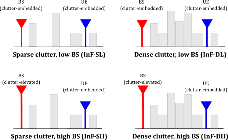
Figure 1: 3GPP Indoor Factory sub-scenarios.

With the rise of Industry 4.0, mobile stations have become a requisite for a smooth and flexible factory operation. In a future factory, for example, one can expect to have workers connected to the factory network, mobile robots being used for remote access and to provide connectivity in emergency cases, automated guided vehicles (AGV) for loading and unloading items, amongst dozens of other possible mobile stations. This mixed and flexible environment creates a challenging scenario for mobility optimization and may require sophisticated techniques. Each factory floor is unique and different from others. Hence, there are no one-size-fits-all mobility parameters, which is why site-specific mobility optimization is needed.

The 3GPP TR 38.901 [26] proposes the Indoor Factory (InF) channel model that focuses on considering factory halls and the presence of “clutter”, e.g.: machinery of different sizes, assembly lines, and storage shelves, of various density and size. Unlike other 3GPP indoor models in which a non-line-of-sight (NLOS) condition is mainly caused by internal walls, people transiting, and office material, in InF, NLOS is defined as a function of the BS and UEs heights and clutter density. Depending on the height, the BS and UE can be considered as clutter embedded or clutter elevated, and depending on the density of clutter, the scenario can be considered as dense or sparse. Finally, there are four possible sub-scenarios to be considered as shown in Fig. 1: Sparse clutter, low BS (InF-SL); Dense clutter, low BS (InF-DL); Sparse clutter, high BS (InF-SH); and Dense clutter, high BS (InF-DH), aside from the line-of-sight case with both UE and BS elevated.

TABLE I: InF sub-scenario specific parameters

	InF-SL	InF-DL	InF-SH	InF-DH
UE height $h_{UE}$ [m]	1.5	1.5	1.5	1.5
BS height $h_{BS}$ [m]	1.5	1.5	8	8
Clutter size $d_{\text{clutter}}$ [m]	10	2	10	2
Clutter density $r$ [%]	20	80	20	80
Clutter height $h_{c}$ [m]	2	6	2	6
Shadowing standard
deviation $\sigma$[dB]	5.7	7.2	5.9	4.0

The LOS probability determines the likelihood of a link to be in LOS or NLOS at a certain distance. The InF LOS probability is given as follows:

$$\Pr\{LOS\}=\exp{\left(-\frac{d_{2D}}{k}\right)},$$ (4)

where

$$k=\left\{\begin{matrix}-\frac{d_{\text{clutter}}}{\ln{\left(1-r\right)}}&\mathrm{for\ InF-SL,InF-DL}\\ -\frac{d_{\text{clutter}}}{\ln{\left(1-r\right)}}.\frac{h_{BS}-h_{UE}}{h_{c}-h_{UE}}&\mathrm{for\ InF-SH,InF-DH}\\ \end{matrix}\right.$$ (5)

and (4) accounts for the blockage caused by machinery through the clutter size $d_{\text{cutter}}$, the clutter density $r$, and UE and BS antennas height $h_{UE}$ and $h_{BS}$, respectively. Note that $k$ increases with the clutter density when the BS antenna is higher than the clutter, whereas the opposite occurs for a BS antenna lower than the clutter [27]. The scenario-specific parameters are summarized in Table I. Details on the LOS and NLOS pathloss models can be found in [26].

III-B System Model

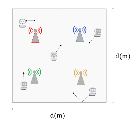
Figure 2: Illustration of the Indoor Factory scenario considered.

For assessing the gains obtained by the proposed MOBO methodology, we consider the $d\times d$ indoor factory scenario depicted in Fig. 2, with $d=40~{}m$. This scenario contains ten mobile UEs randomly dropped in the area and four fixed-position BSs separated by a distance $d/2$. The height of BSs and UEs, as well as the clutter height, density, and size, all depend on the 3GPP-InF sub-scenario considered and are summarized in Table I.

Both UEs and BSs are equipped with one omnidirectional antenna and UEs associate with the BSs providing the highest received signal strength (RSS), which is recomputed each time the UE moves to the next position. As for the mobility model, we assume that UEs move on a straight line with a random departure angle, bouncing back when reaching the scenario’s boundaries. We observe HO failures happening in a window of 250 s, with a time step of 0.5 s and a baseline UE velocity of 5 km/h.

Pathloss and shadowing are modeled following the 3GPP InF standard. In this problem, mobility decisions are based on large-scale fading whereby the effect of small-scale fading is averaged out [28]. The system operates at a carrier frequency of 3.5 GHz and the BS transmission power is set to 30 dBm, with a transmission bandwidth of 100 MHz [26]. The main simulation parameters are listed in Table II.

TABLE II: Simulation parameters

General parameters
Monte Carlo samples	300
Number of UEs	10
Number of BSs	4
Scenario size [m]	40
Channel model	3GPP InF-DH [26]
Noise spectral density [dB/MHz]	-174
Noise figure UEs [dB]	9
Bandwidth [MHz]	100
TX power BSs [dBm]	30
$f_{c}$ [GHz]	3.5
RFL power threshold [dBm]	-90
SINR RLF threshold [dB]	-5
BS height [m]	8
UE height [m]	1.5
UE speed [km/h]	5
HO threshold [dB]	[-5,…,10]
Mobility model	Straight line with random angle
MOBO-specific parameters
Reference point	[200, 200]
Number of full loops	10
Batch size	4 points
Number of batches	25

IV Performance Evaluation

In this section, we present and discuss our simulation results. As mentioned previously, the choice of HO parameters is usually made by the network operator based on expert knowledge. To simulate this approach as a benchmark, we consider an exhaustive search baseline in which HO thresholds from -5 dB to 10 dB are tested on each of the four InF sub-scenarios, and the number of HO failures over 250 seconds is observed. For statistical purposes, each HO threshold configuration is tested in 300 MC simulations. In each MC simulation, UEs are randomly re-dropped and moved with a fixed speed of 5 km/h. The MOBO algorithm is run using the BoTorch framework [29], which is a library for Bayesian Optimization built atop PyTorch. We refer to a full optimization loop as a complete run of MOBO, from initial sample generation to a final recommendation; the each full loop contains $b$ batches of $q$ candidate points to be evaluated in the surrogate model. In this problem, each objective is modeled as an independent GP with a Matérn 5/2 kernel, and the multi-objective problem is optimized using the $q$EHVI acquisition function.

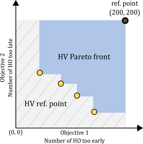
Figure 3: Illustration of hypervolume considering the problem of minimizing both the number of HOs too early and too late and assuming a reference point of (200, 200) as being the maximum number of acceptable HO failures.

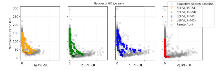
Figure 4: Complete search space with all samples obtained through exhaustive search vs the samples points by MOBO for the four channel models considered.

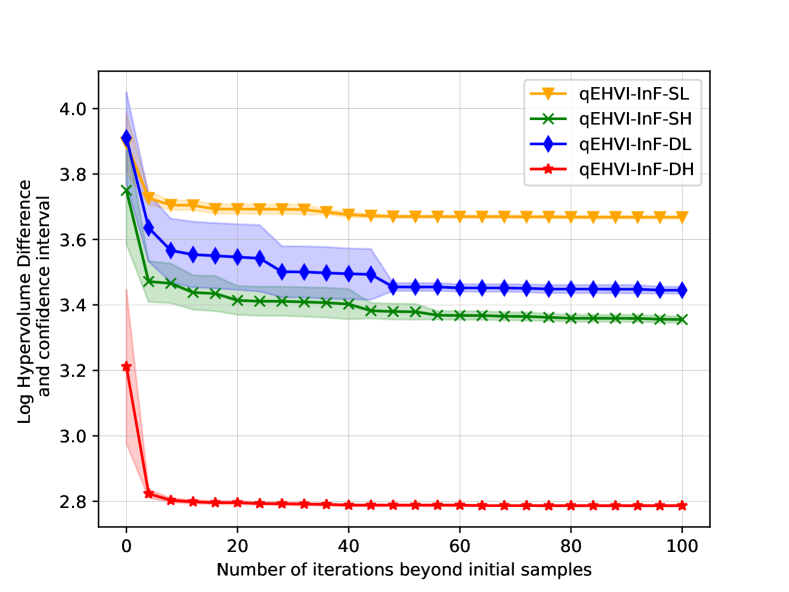
Figure 5: Log HV difference of the solution found by MOBO-$q$EHVI for all of the InF sub-scenarios (markers) and confidence interval (shaded areas).

A solid metric of the convergence and quality of a multi-objective problem’s solution is the hypervolume (HV) [30], i.e., the multi-dimensional volume of the region dominated by a set of solutions and bounded by a specified reference point. The log hypervolume difference is the log difference between the HV covered by the reference point and the HV of the approximated Pareto front obtained through MOBO as follows:

$$\log_{10}\text{HV}_{\text{diff}}=\log_{10}(\text{HV}_{\text{ref. point}}-\text{HV}_{\text{MOBO}}).$$ (6)

In this paper, we consider as a reference point the maximum number of acceptable HO failures, namely 200 HOs too early/late, and define the latter as the bound in the MOBO algorithm. Fig. 3 helps to visualize the HV calculation. Fig. 5 shows the log hypervolume difference for the solutions found by the MOBO algorithm per iteration, averaged over 10 trials. The proposed algorithm reaches convergence in less than 50 iterations for all scenarios tested, determining the Pareto front.

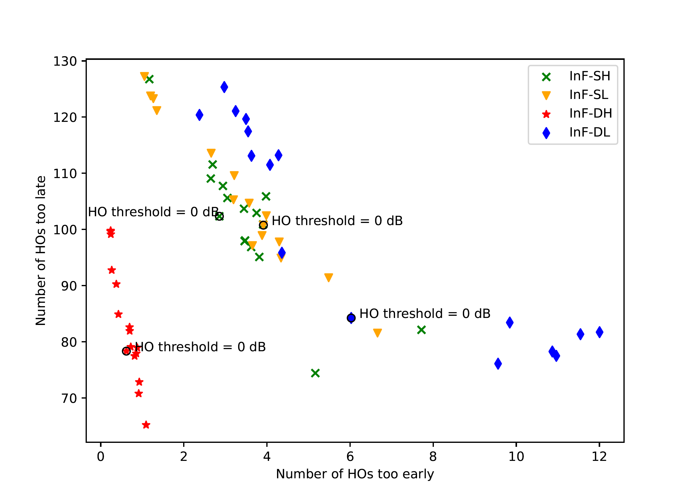
Figure 6: MOBO posterior model mean for all the InF sub-scenarios.

Fig. 4 shows the full search space used by BO and the baseline exhaustive search approach. In this baseline, we observe all possible HO thresholds over 300 MC samples for each value, whereas MOBO runs 10 full optimization loops with $b$ = 25 batches of $q$ = 4 candidate points in each batch. The value of $q$ was chosen for the sake of complexity, as the optimization complexity increases with $q$. We note how MOBO samples points with lower variance, closer to the approximated Pareto front for all the InF sub-scenarios, and can find a sub-optimal solution using fewer samples than the baseline exhaustive search. The latter is able to eventually find solutions closer to zero-failures, but at the cost of requiring more samples and testing undesirable operating points that can dangerously jeopardize the system’s performance. Although there is no guarantee that MOBO will never make a decision that can degrade the network performance, the search space in MOBO is safely restricted, i.e., worst-case limits can be set as parameters before the optimization with an error margin. In this problem, the limit was set to 200 HO failures, but was never reached by MOBO, showing its robustness and safe exploration.

Fig. 6 shows an average over 10 trials of the posterior models learned by the MOBO algorithm for each HO threshold tested. The posterior distribution is used for estimating the posterior value of the black-box function given a data sample, and this distribution is used to decide which point to sample next. Note that the models are only an approximation of the true objective function and the MOBO algorithm focuses on sampling points closer to the approximate Pareto front, therefore the “non-monotonic” behavior in Fig. 6 can be caused by the optimization process’s outliers. It is possible to reach a smoother curve by increasing the number of trials, but we choose to limit the number of trials to showcase that MOBO only needs a few iterations for convergence and can operate even with noisy data samples. The models learned can also be used as a starting point for future optimization adjustments.

V Conclusions

In this paper, we formulated a multi-objective optimization problem for determining the HO threshold that minimizes both the number of HOs too early and too late in various 3GPP indoor factory scenarios. We then used multi-objective Bayesian Optimization to solve the problem and evaluated the performance of the MOBO algorithm against a baseline exhaustive search. Our results showed that, although exhaustive search can reach a solution closer to zero, it does so at the cost of needing more sample points and exploring parameters that can drastically degrade the system’s performance. Instead, MOBO reaches a Pareto optimal solution with fewer samples and guarantees a safer exploration, ensuring sustained QoS.

We also showed that the model learned by MOBO has a high confidence interval even when using noisy data. While GP is usually the favorite choice of surrogate model, the problem at hand deals with discrete counters and its posterior model may be better estimated through a discrete surrogate model. A promising research direction is thus employing discrete models such as Random Forests or Beta-Bernoulli bandits.

In practical scenarios, implementing MOBO with $q$EHVI would entail the parallel evaluation of the multiple candidate points generated. This could be accomplished either (i) evaluating the points in parallel by creating subsets of users to test each of the candidate points, or (ii) testing the points sequentially using the entire network. The latter approach would still yield a performance advantage since $q$EHVI samples multiple candidate points at the same time, thus requiring fewer steps to maximize the acquisition function than a fully sequential optimization approach.

References

- [1] M. Tayyab, X. Gelabert, and R. Jäntti, “A survey on handover management: From LTE to NR,” IEEE Access, vol. 7, pp. 118 907–118 930, 2019.
- [2] M. S. Mollel et al., “A survey of machine learning applications to handover management in 5G and beyond,” IEEE Access, vol. 9, pp. 45 770–45 802, 2021.
- [3] A. Masri et al., “Machine-learning-based predictive handover,” in 2021 IFIP/IEEE International Symposium on Integrated Network Management (IM). IEEE, 2021, pp. 648–652.
- [4] “Evolved Universal Terrestrial Radio Access (E-UTRA) and NR; Study on enhancement for Data Collection for NR and EN-DC (Release 17),” 3GPP TR 37.817, January 2022.
- [5] V. Yajnanarayana, H. Ryden, and L. Hevizi, “5G Handover using Reinforcement Learning,” 2020 IEEE 3rd 5G World Forum, 5GWF 2020 - Conference Proceedings, pp. 349–354, 2020.
- [6] J. Tanveer, A. Haider, R. Ali, and A. Kim, “An Overview of Reinforcement Learning Algorithms for Handover Management in 5G Ultra-Dense Small Cell Networks,” Applied Sciences, vol. 12, no. 1, 2022.
- [7] Ş. Sönmez, I. Shayea, S. A. Khan, and A. Alhammadi, “Handover management for next-generation wireless networks: A brief overview,” IEEE Microwave Theory and Techniques in Wireless Communications, vol. 1, pp. 35–40, 2020.
- [8] M. B. Yassein, S. Aljawarneh, and W. Al-Sarayrah, “Mobility management of internet of things: Protocols, challenges and open issues,” in Proc. International Conference on Engineering & MIS, 2017, pp. 1–8.
- [9] M. U. B. Farooq, M. Manalastas, S. M. A. Zaidi, A. Abu-Dayya, and A. Imran, “Machine learning aided holistic handover optimization for emerging networks,” arXiv preprint arXiv:2202.02851, 2022.
- [10] S. A. Khan et al., “An improved handover decision algorithm for 5G heterogeneous networks,” Proc. IEEE Malaysia International Conference on Communications, pp. 25–30, 2021.
- [11] W. Huang, M. Wu, Z. Yang, K. Sun, H. Zhang, and A. Nallanathan, “Self-Adapting Handover Parameters Optimization for SDN-Enabled UDN,” IEEE Transactions on Wireless Communications, 2022.
- [12] M. R. Palas et al., “Multi-criteria handover mobility management in 5G cellular network,” Computer Communications, vol. 174, pp. 81–91, 2021.
- [13] S. Chang et al., “Individualized optimization of handover parameters in 5G (NR) indoor and outdoor co-frequency scenarios,” Proc. IEEE ICCECE, pp. 59–66, 2021.
- [14] P. C. Lin, L. F. Casanova, and B. K. Fatty, “Data-Driven Handover Optimization in Next Generation Mobile Communication Networks,” Mobile Information Systems, vol. 2016, 2016.
- [15] Y. Ma, X. Chen, and L. Zhang, “Base Station handover Based on User Trajectory Prediction in 5G Networks,” 19th IEEE International Symposium on Parallel and Distributed Processing with Applications, pp. 1476–1482, 2021.
- [16] R. M. Dreifuerst et al., “Optimizing coverage and capacity in cellular networks using machine learning,” in Proc. IEEE ICASSP, 2021, pp. 8138–8142.
- [17] L. Maggi, A. Valcarce, and J. Hoydis, “Bayesian optimization for radio resource management: Open loop power control,” IEEE Journal on Selected Areas in Communications, vol. 39, no. 7, pp. 1858–1871, 2021.
- [18] R. Hassan, A. H. M. Aman, L. A. Latiff et al., “Framework for handover process using visible light communications in 5G,” in Proc. Symposium on Future Telecommunication Technologies, vol. 1, 2019, pp. 1–4.
- [19] Y. Lu et al., “Feasibility of location-aware handover for autonomous vehicles in industrial multi-radio environments,” Sensors, vol. 20, no. 21, p. 6290, 2020.
- [20] D. Li, X. Li, and J. Wan, “A cloud-assisted handover optimization strategy for mobile nodes in industrial wireless networks,” Computer Networks, vol. 128, pp. 133–141, 2017.
- [21] A. S. Gaur, J. Budakoti, C.-H. Lung et al., “Vertical handover decision for mobile iot edge gateway using multi-criteria and fuzzy logic techniques,” Advances in Internet of Things, vol. 10, no. 04, p. 57, 2020.
- [22] S. Santi, F. Lemic, and J. Famaey, “Location-based Discovery and Network Handover Management for Heterogeneous IEEE 802.11 ah IoT Applications,” IEEE Trans. Network and Service Management, 2022.
- [23] B. Shahriari, K. Swersky, Z. Wang, R. P. Adams, and N. De Freitas, “Taking the human out of the loop: A review of bayesian optimization,” Proceedings of the IEEE, vol. 104, no. 1, pp. 148–175, 2015.
- [24] C. E. Rasmussen, “Gaussian processes in machine learning,” in Summer school on machine learning. Springer, 2003, pp. 63–71.
- [25] S. Daulton, M. Balandat, and E. Bakshy, “Differentiable expected hypervolume improvement for parallel multi-objective bayesian optimization,” Advances in Neural Information Processing Systems, vol. 33, pp. 9851–9864, 2020.
- [26] (2019) Study on channel model for frequencies from 0.5 to 100 GHz (Release 16). [Online]. Available: https://www.3gpp.org
- [27] T. Jiang et al., “3GPP standardized 5G channel model for IIoT scenarios: A survey,” IEEE Internet of Things Journal, vol. 8, no. 11, pp. 8799–8815, 2021.
- [28] D. Lopez-Perez, I. Guvenc, and X. Chu, “Mobility management challenges in 3gpp heterogeneous networks,” IEEE Communications Magazine, vol. 50, no. 12, pp. 70–78, 2012.
- [29] M. Balandat et al., “Botorch: a framework for efficient monte-carlo bayesian optimization,” Advances in neural information processing systems, vol. 33, pp. 21 524–21 538, 2020.
- [30] N. Riquelme, C. Von Lücken, and B. Baran, “Performance metrics in multi-objective optimization,” in 2015 Latin American computing conference (CLEI). IEEE, 2015, pp. 1–11.