Nonequilibrium Seebeck effect and thermoelectric efficiency
of Kondo-correlated molecular junctions

Abstract

We theoretically study the nonequilibrium thermoelectric transport properties of a strongly-correlated molecule (or quantum dot) embedded in a tunnel junction. Assuming that the coupling of the molecule to the contacts is asymmetric, we determine the nonlinear current driven by the voltage and temperature gradients by using the perturbation theory. However, the subsystem consisting of the molecule strongly coupled to one of the contacts is solved by using the numerical renormalization group method, which allows for accurate description of Kondo correlations. We study the temperature gradient and voltage dependence of the nonlinear and differential Seebeck coefficients for various initial configurations of the system. In particular, we show that in the Coulomb blockade regime with singly occupied molecule, both thermopowers exhibit sign changes due to the Kondo correlations at nonequilibrium conditions. Moreover, we determine the nonlinear heat current and thermoelectric efficiency, demonstrating that the system can work as a heat engine with considerable efficiency, depending on the transport regime.

I Introduction

Thermoelectric properties of nanoscale systems have become a subject of extensive studies [1, 2, 3, 4]. This is because such structures, due to their reduced dimensions, allow for obtaining thermal response much exceeding that obtained in bulk materials [5]. In this regard, a special role is played by zero-dimensional systems, such as molecules or quantum dots, in which discrete energy spectrum is relevant for efficient energy filtering and obtaining considerable figure of merit. Thermopower of such systems has already been explored theoretically [6, 7, 8, 9, 10, 11], both in the weak and strong coupling regimes, as well as experimentally [12, 13, 14]. A special attention has been paid to strong electron correlation regime, where the Kondo effect can emerge at sufficiently low temperatures [15, 16]. This is due to the fact that the analysis of the temperature dependence of the Seebeck effect can provide additional information about the Kondo correlations in the system [9, 13, 14]. In particular, sign changes of linear thermopower as a function of temperature were shown to indicate the onset of the Kondo correlations in the system [13, 14]. From theoretical side, accurate description of thermoelectric phenomena in the strong correlation regime requires using sophisticated numerical methods, therefore such considerations have been mostly limited to the linear response regime [9, 17, 18, 19, 20, 21], while much less attention has been paid to the far-from-equilibrium regime [22, 11].

The goal of this work is therefore to shed more light on the nonequilibrium thermoelectric characteristics in systems where Kondo correlations are crucial. For that, we consider a molecule (or a quantum dot) asymmetrically attached to external contacts. Such system’s geometry allows us to incorporate strong electron correlation effects in far-from-equilibrium conditions in a very accurate manner. The electronic correlations give rise to the development of the Kondo phenomenon, which arises due to the strong coupling to one of the contacts, whereas the second contact, serves as a weakly coupled probe. In such scenario, we can make use of the numerical renormalization group (NRG) method [23, 24, 25] to solve the strongly-coupled subsystem, while the nonequilibrium current flowing through the whole system, triggered by voltage and/or temperature gradients, is evaluated based on the perturbation theory with respect to the weakly attached electrode. We show that with this method we can determine the thermoelectric effects at large and finite temperature and potential gradient without losing the Kondo correlations. We also note that accurate quantitative calculation of nonequilibrium thermoelectric transport in the case of symmetrically-coupled systems poses a great challenge that could be addressed by recently developed hybrid approach involving time-dependent density matrix renormalization group and NRG [26, 27].

For the considered system here, we first study the voltage dependence of the differential conductance, demonstrating suppression of the zero-bias Kondo peak with increasing the temperature gradient. We then focus on the analysis of nonequilibrium and differential Seebeck effects, analyzing at the beginning the case of finite temperature gradient within linear response in applied voltage. Furthermore, we examine the behavior of the thermopower in the nonlinear voltage and temperature gradient regime, predicting new sign changes associated with Kondo correlations. We also calculate the heat currents and the power generated by the device as well as the corresponding thermoelectric efficiency, revealing regimes of large efficiency depending on the transport regime. Finally, assuming realistic junction parameters, we consider the thermoelectric transport properties including the voltage dependence of the molecule’s orbital level.

The paper is organized as follows. In Sec. II, we discuss the model and method used in the calculations along with the definitions for thermopower in out-of-equilibrium settings. The main results and discussions are presented in Sec. III, which begins with the analysis of the electronic transport under a finite potential bias and temperature gradient. The nonequilibrium thermoelectric coefficients are then studied, first at zero-bias, and then generalized to the finite bias and temperature conditions. We also determine the behavior of the nonequilibrium heat current and the thermoelectric efficiency of the system under various parameter regimes. Finally, the paper is summarized in Sec. IV.

II Theoretical Framework

II.1 Model and Hamiltonian

The considered system consists of a molecule (or a quantum dot) asymmetrically coupled to two metallic leads, as schematically shown in Fig. 1. The molecule is described by an orbital level of energy $\varepsilon_{d}$ and Coulomb correlations denoted by $U$. This orbital level may correspond to the lowest unoccupied orbital level (LUMO level) of the molecule. Transport through the system can be induced and controlled by applying a finite bias voltage $V$ and/or a temperature gradient $\Delta T$ across the leads. We assume that the left contact is grounded and kept at a constant temperature $T$, while the right contact is subject to $V$ and $\Delta T$, see Fig. 1. The temperature $T$ is assumed to be much smaller than the characteristic energy scale of the Kondo effect, i.e. in practical calculations we set $T\to 0$. Moreover, it is assumed that the coupling to the left lead ($\Gamma_{L}$) is much stronger than the coupling to the right electrode ($\Gamma_{R}$). Such an asymmetry is frequently present in various molecular junctions [28, 29, 30, 31, 32], it can be also generated in artificial heterostructures comprising e.g. a quantum dot [33, 34, 35]. Furthermore, it can be also encountered in studies of adatoms with scanning tunneling spectroscopy. Under this assumption, we determine the current flowing through the system using the perturbation theory in $\Gamma_{R}$, while the subsystem consisting of molecule strongly coupled to the left lead is treated exactly with the aid of the numerical renormalization group method [23, 24, 25]. In other words, we include the lowest-order processes between the molecule and the right electrode, while the tunneling processes between the molecule and the left lead are taken into account in an exact manner.

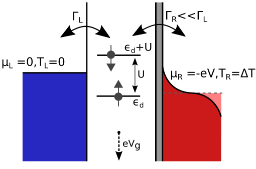
Figure 1: The schematic of the considered system. It consists of a molecule (or a quantum dot) characterized by an orbital level of energy $\varepsilon_{d}$ and Coulombic repulsion $U$. The molecule is strongly coupled to the left lead with coupling strength $\Gamma_{L}$, while the coupling to the right contact $\Gamma_{R}$ is much weaker. $V_{g}$ stands for the gate voltage, which can be used to tune the position of the orbital level. $\mu_{L}$ ($\mu_{R}$) and $T_{L}$ ($T_{R}$) denote the chemical potential and temperature of the left (right) lead, respectively. The left contact is grounded and kept at a constant temperature $T_{L}=0$, while the right contact is subject to voltage bias $V$ and temperature gradient $\Delta T$.

The Hamiltonian of the molecule coupled to the left lead can be expressed as [36]

$$H_{L} = \varepsilon_{d}n+Un_{\uparrow}n_{\downarrow}+\sum_{k\sigma}\varepsilon_{Lk\sigma}c^{\dagger}_{Lk\sigma}c_{Lk\sigma}$$ (1)

$$+\sqrt{\frac{\Gamma_{L}}{\pi\rho_{L}}}\sum_{k\sigma}(d^{\dagger}_{\sigma}c_{Lk\sigma}+c^{\dagger}_{Lk\sigma}d_{\sigma}),$$

where the first two terms model the orbital level with energy $\varepsilon_{d}$ and Coulomb correlations $U$, with $n=n_{\uparrow}+n_{\downarrow}$, $n_{\sigma}=d_{\sigma}^{\dagger}d_{\sigma}$, and $d_{\sigma}^{\dagger}$ ($d_{\sigma}$) being the creation (annihilation) operator for spin-$\sigma$ electrons on the orbital level. The creation (annihilation) operator for an electron of spin $\sigma$, momentum $k$ and energy $\varepsilon_{\alpha k\sigma}$ in the lead $\alpha$ is denoted by $c_{\alpha k\sigma}^{\dagger}$ ($c_{\alpha k\sigma}$). The third term in Eq. (1) describes the left lead in the free quasiparticle approximation, while the last term models the tunneling processes between the molecule and left lead. The density of states of the lead $\alpha$ is described by $\rho_{\alpha}$. Here we use the wide-band approximation under which the couplings are energy independent. On the other hand, the Hamiltonian of the right contact can be written as [37],

$$H_{R}=\sum_{k\sigma}\varepsilon_{Rk\sigma}c^{\dagger}_{Rk\sigma}c_{Rk\sigma}-eV\sum_{k\sigma}c^{\dagger}_{Rk\sigma}c_{Rk\sigma},$$ (2)

where $V$ is the applied bias voltage and $e$ stands for the elementary charge. Then, the tunneling processes between the left and right part of the system can be described by the following tunneling Hamiltonian [37]

$$H_{T}=\sqrt{\frac{\Gamma_{R}}{\pi\rho_{R}}}\sum_{k\sigma}(d^{\dagger}_{\sigma}c_{Rk\sigma}+c^{\dagger}_{Rk\sigma}d_{\sigma}).$$ (3)

Thus, the total Hamiltonian is given by a sum of three terms, the strongly coupled left part, $H_{L}$, the weakly coupled right lead, $H_{R}$, and the term accounting for tunneling between both parts, $H_{T}$, $H=H_{L}+H_{R}+H_{T}$. In what follows, to determined the tremoelectric transport properties, we perform a perturbation expansion in $H_{T}$.

II.2 Nonequilibrium transport coefficients

II.2.1 Electric current

The assumption of the weak coupling $\Gamma_{R}$ to the right subsystem allows us to perform a perturbative expansion in $H_{T}$. In the lowest-order perturbation theory, the electric current $I(V,\Delta T)$ at voltage bias $V$ and temperature gradient $\Delta T$ can be expressed as [33, 35]

$$I(V,\Delta T) = -\frac{2e\Gamma_{R}}{\hbar}\!\int_{-\infty}^{\infty}\!d\omega A_{L}(\omega)\times$$ (4)

$$\left[f_{L}(\omega)-f_{R}(\omega-eV)\right],$$

where $A_{L}(\omega)$ is the local density of states (spectral function) of the left subsystem and $f_{\alpha}(\omega)$ denotes the Fermi-Dirac distribution function of the lead $\alpha$, ${f_{\alpha}(\omega)={[1+\textrm{exp}(\omega/T_{\alpha})]^{-1}}}$, with $T_{L}=0$ and $T_{R}=\Delta T$, cf. Fig. 1, and $k_{B}\equiv 1$. The factor of $2$ in Eq. (11) results from the spin degrees of freedom.

The spectral function $A_{L}(\omega)$ of the left subsystem is calculated by using the numerical renormalization group method [23, 24, 25]. This method is well-suited to account for electron correlations in a very accurate manner, and especially those giving rise to the Kondo effect [16]. The spectral function can be related to the imaginary part of the molecule’s orbital level retarded Green’s function $G^{r}_{\sigma}(\omega)$, $A_{L}(\omega)=\sum_{\sigma}A_{L\sigma}(\omega)$, with $A_{L\sigma}(\omega)=-{\rm Im}G^{r}_{\sigma}(\omega)/\pi$, where $G^{r}_{\sigma}(\omega)$ is the Fourier transform of $G^{r}_{\sigma}(t)=-i\Theta(t)\langle\{d_{\sigma}(t),d_{\sigma}^{\dagger}(0)\}\rangle$. Within the NRG, we first determine the eigenspectrum of $H_{L}$ and then calculate $A_{L}(\omega)$ in the Lehmann representation. In addition, to improve the quality of the spectral data, we also employ the z-averaging approach [38].

II.2.2 Seebeck coefficient

A special emphasis in this paper is put on the nonequilibrium behavior triggered by a large temperature and/or voltage gradient. The Seebeck coefficient (or thermopower) is the thermoelectric property that quantifies the voltage induced by a thermal gradient across a conductor, and is defined as,

$$S=-\left(\frac{V}{\Delta T}\right)_{\!\!I=0},$$ (5)

under the assumption that the current $I$ through the system vanishes, $I=0$.

In the linear response regime, the Seebeck coefficient, $S_{\rm lin}$, can be reliably described by using the Onsager integrals, ${L_{n}=-\frac{1}{h}\int d\omega\;\omega^{n}f^{\prime}(\omega)\mathcal{T}(\omega)}$, involving the transmission coefficient, $\mathcal{T}(\omega)\propto\Gamma_{R}\,A_{L}(\omega)$, where $f^{\prime}(\omega)$ is the derivative of the Fermi function [39]

$$S_{\rm lin}=-\frac{1}{eT}\frac{L_{1}}{L_{0}}.$$ (6)

This basic definition of the Seebeck coefficient can be directly extended to the nonequilibrium case by considering that only the current generated by the thermal gradient must vanish. Assume, for example, that a system with potential bias $V$ exhibits a current $I$ flowing through it. When an additional temperature gradient $\Delta T$ is applied, a new current $I_{\rm tot}=I+I_{\rm th}$ will flow through the system, where $I_{\rm th}$ is the additional current induced by the thermal gradient. One can then define a nonequilibrium (nonlinear) Seebeck coefficient $S_{\rm n}(V,\Delta T)$ as [40, 41, 42, 43, 44, 43, 34, 11]

$$S_{\rm n}(V,\Delta T)=-\left(\frac{\Delta V}{\Delta T}\right)_{\!\!I(V+\Delta V,\Delta T)=I(V,0)},$$ (7)

where $\Delta V$ is the change in potential bias required to suppress the current induced by the thermal gradient $\Delta T$.

Additionally, in the nonlinear response regime, one can also define a differential Seebeck coefficient $S_{\rm d}(V,\Delta T)$ as [45]

$$S_{\rm d}(V,\Delta T)=-\!\left(\frac{dV}{d\Delta T}\!\right)_{\!\!I}\!=-\!\left(\frac{\partial I}{\partial\Delta T}\!\right)_{\!\!V}\bigg{/}\!\!\left(\frac{\partial I}{\partial V}\!\right)_{\!\!\Delta T},$$ (8)

where $\left(\frac{\partial X}{\partial Y}\right)_{\!Z}$ describes the partial derivative of $X$ with respect to $Y$, while keeping $Z$ constant. The differential Seebeck effect is related to the ratio of the thermal response at finite voltage to differential conductance at finite temperature gradient. We note that in the linear response regime with respect to the bias voltage, $S_{\rm d}$ becomes comparable to the linear response Seebeck coefficient given by Eq. (6).

II.2.3 Heat current and thermoelectric efficiency

We are also interested in the behavior of the nonequilibrium heat current and the thermoelectric efficiency $\eta$ [46, 47, 48, 49, 50, 51]. The formula for the heat current can be derived from the first law of thermodynamics, which for subsystem $\alpha=L,R$ reads, $dU_{\alpha}=dW_{\alpha}+dQ_{\alpha}$. Here, $dU_{\alpha}$ is the energy flowing into the subsystem $\alpha$, while $dQ_{\alpha}$ denotes the corresponding heat. The work done to the subsystem $\alpha$ is generally given by, $dW_{\alpha}=\mu_{\alpha}dN_{\alpha}$, where $dN_{\alpha}$ is the corresponding particle number change. The heat current associated with the left and right subsystem can be then defined as [47]

$$I_{L}^{Q}(V,\Delta T) = I^{E}(V,\Delta T)-\mu_{L}I(V,\Delta T)/e,$$ (9)

$$I_{R}^{Q}(V,\Delta T) = I^{E}(V,\Delta T)-\mu_{R}I(V,\Delta T)/e,$$ (10)

where $I^{E}(V,\Delta T)$ denotes the energy current given by

$$I^{E}(V,\Delta T) = -\frac{2\Gamma_{R}}{\hbar}\!\int_{-\infty}^{\infty}\!d\omega\;\omega\;A_{L}(\omega)\times$$ (11)

$$\left[f_{L}(\omega)-f_{R}(\omega-eV)\right].$$

In our setup, $T_{R}>T_{L}$, see Fig. 1, such that the electrons flow from the hot reservoir to the cold one performing the work $\dot{W}(V,\Delta T)$ per unit time. Such power output can be related to the heat currents through

$$P\equiv\dot{W}(V,\Delta T)=I_{R}^{Q}(V,\Delta T)-I_{L}^{Q}(V,\Delta T).$$ (12)

Then, the thermoelectric efficiency of such a heat engine can be defined as the ratio of the power to the heat extracted from the hot reservoir

$$\eta(V,\Delta T)=\frac{\dot{W}(V,\Delta T)}{I_{R}^{Q}(V,\Delta T)}=1-\frac{I_{L}^{Q}(V,\Delta T)}{I_{R}^{Q}(V,\Delta T)}.$$ (13)

III Results and discussion

In this section we present and discuss the numerical results obtained for the differential conductance and Seebeck effect in far-from-equilibrium conditions. For the considered system we assume the Coulomb correlations, $U=0.2$, the coupling to the left lead, $\Gamma_{L}=0.02$, in units of half bandwidth, while the weak coupling to the right lead is assumed to be, $\Gamma_{R}=\Gamma_{L}/10$. In NRG calculations we keep at least $4^{5}$ states in the iterative procedure and perform averaging over $8$ different discretizations [38].

We note that in experimentally relevant scenarios, a voltage drop imposed across the junction would result in a change of the orbital level, depending on capacitive couplings to the contacts and to the gate voltage. However, to get a better understanding of the transport properties, we first assume that the position of the orbital level does not change as the bias voltage is tuned. This would correspond to immediately counterbalancing the voltage drop on the molecule by an appropriate tuning of the gate voltage. Nevertheless, further on, assuming exemplary parameters of the junctions, we also present the results for the case when the orbital level depends on the transport voltage.

III.1 Electronic transport under finite potential and temperature gradient

Figure 2: The differential conductance plotted as a function of the bias voltage $V$ for different values of the temperature gradient $\Delta T$, as indicated. The inset shows the evolution of the zero-bias conductance as a function of $\Delta T$. The parameters are: $U=0.2$, $\Gamma_{L}=0.02$, $\Gamma_{R}=0.002$, $T=0$, in units of band halfwidth, and $\varepsilon_{d}=-0.3\,U$. The Kondo temperature can be estimated from the Haldane’s formula, which for assumed parameters yields $T_{K}/U\approx 8.26\cdot 10^{-3}$. The Kondo energy scale in the applied bias potential, defined as the half-width at half-maximum of the $G(V)$ curve, is found to be $eV_{K}/U\approx 1.45\cdot 10^{-2}$.

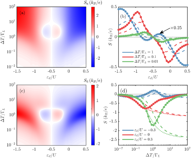
Figure 3: (a) The non-equilibrium Seebeck coefficient $S_{\rm n}$ and (c) the differential Seebeck coefficient $S_{\rm d}$ calculated as a function of the orbital energy $\varepsilon_{d}$ and the temperature gradient $\Delta T$ at potential bias $V\to 0$ for parameters the same as in Fig. 2. Note the logarithmic scale in temperature gradient. (b) shows the horizontal cross-sections of (a) and (c), i.e., the dependence of $S_{\rm n}$ (dashed) and $S_{\rm d}$ (solid) as a function of $\varepsilon_{d}$ for various $\Delta T$, whereas (d) presents the vertical cross-sections of (a) and (c), i.e., the dependence of $S_{\rm n}$ (dashed) and $S_{\rm d}$ (solid) on $\Delta T$ for various $\varepsilon_{d}$. The colored circles show the linear response thermopower $S_{\rm lin}(T=\Delta T)$ and the colored dotted lines in (d) show the rescaled non-equilibrium thermopower $S_{\rm n}(2\,\Delta T)$.

Let us first analyze the behavior of the differential conductance $G\equiv dI(V,\Delta T)/dV$ as a function of the bias voltage calculated for different temperature gradients $\Delta T$. This dependence is presented in Fig. 2. The figure was generated for $\varepsilon_{d}=-0.3\,U$, i.e. in the local moment regime, where the system exhibits the Kondo effect caused by the strong coupling to the left contact. The relevant Kondo temperature for the left subsystem can be estimated from the Haldane’s formula [52], which yields, $T_{K}\approx 8.26\cdot 10^{-3}\,U=8.26\cdot 10^{-2}\,\Gamma_{L}$. Note that because $\Gamma_{R}=\Gamma_{L}/10$, the Kondo temperature associated with the right contact is exponentially suppressed and thus negligible. The presence of Kondo correlations is reflected in a pronounced zero-bias peak visible in the differential conductance, see Fig. 2. Note that because of asymmetric couplings, the maximum of conductance at zero bias is much reduced compared to $2e^{2}/h$. With increasing the bias voltage, the conductance decreases and shows smaller resonances corresponding to $eV\approx\varepsilon_{d}$ and $eV\approx\varepsilon_{d}+U$. When the thermal gradient increases (note that the base system temperature is assumed to be $T=0$), one observes a gradual suppression of the zero-bias anomaly, until the whole bias dependence of $G$ does not show any Kondo correlation effects for $\Delta T\gg T_{K}$. The evolution of the Kondo peak with increasing $\Delta T$ is explicitly presented in the inset of Fig. 2. The conductance drops to a half of its maximum value when $\Delta T\approx 2T_{K}$. This reflects the fact that the actual system temperature, which can be associated with an average of the left and right contact temperatures, is equal to $\Delta T/2$. We also note that for $\Delta T\ll T_{K}$ one can quantify the Kondo resonance by $V_{K}$, which characterizes the Kondo energy scale in the applied bias potential, defined as the half-width at half-maximum of the $G(V)$ curve. For $V_{K}$ we find, $eV_{K}\approx 1.45\cdot 10^{-2}\,U=1.45\cdot 10^{-1}\,\Gamma_{L}$.

III.2 Non-equilibrium thermopower

In this section we focus on the analysis of the behavior of thermopower, both $S_{\rm n}$ and $S_{\rm d}$, cf. Eqs. (7) and (8), under finite temperature and voltage gradients. However, to get a better understanding of thermoelectric transport, we first start with the case of $V\to 0$, while nonequiliibrium settings are imposed only by increasing $\Delta T$. The more general case of having both finite $\Delta T$ and $V$ will be examined afterwards.

III.2.1 Thermopower under finite temperature gradient

The nonequilibrium $(S_{\rm n})$ and differential $(S_{\rm d})$ Seebeck coefficients as a function of temperature gradient $\Delta T$ and orbital level position $\varepsilon_{d}$, for the case when the nonlinear response regime is triggered by a large temperature gradient, are presented in Fig. 3. Before analyzing the behavior of the thermopower in greater detail, let us first briefly discuss different regimes for the energy of the orbital level $\varepsilon_{d}$, and what it implies. The local moment regime, $-1\lesssim\varepsilon_{d}/U\lesssim 0$, denotes the value of orbital energy, in which the singly occupied level is held below the Fermi energy (of the left electrode in our case) and the doubly occupied state is above the Fermi level. This is the regime where the molecule is occupied by an unpaired electron and the system can exhibit the Kondo effect. As can be inferred from the name, the empty/fully occupied regime, $\varepsilon_{d}/U\gtrsim 0$, $\varepsilon_{d}/U\lesssim-1$, refers to the case where the preferred configuration is having the orbital level completely empty or fully occupied. On the other hand, when $\varepsilon_{d}/U\approx-1$ or $\varepsilon_{d}/U\approx 0$, we reach a mixed valence/resonant tunneling regime where the orbital level is in the vicinity of the Fermi level of the electrode (depending on its hybridization $\Gamma_{L}$).

The colormaps for $S_{\rm n}$ and $S_{\rm d}$ as presented in Figs. 3(a) and (c) show a similar behavior but with interesting deviations. We note that for $V\to 0$ both thermopowers are odd functions of $\varepsilon_{d}$ across the particle-hole symmetry point, $\varepsilon_{d}=-U/2$ [see also Fig. 3(b)], and decay to zero when the temperature gradient $\Delta T\rightarrow 0$ [see also Fig. 3(d)]. Moreover, both $S_{\rm n}$ and $S_{\rm d}$ are generally negative (positive) for $\varepsilon_{d}>-U/2$ ($\varepsilon_{d}<-U/2$), indicating a dominant role of the electron (hole) processes. When inside the local moment regime, both $S_{\rm n}$ and $S_{\rm d}$ survive to even lower values of temperature gradient $\Delta T/\Gamma_{L}\approx 10^{-2}$, compared to $\Delta T/\Gamma_{L}\approx-10^{-1}$, as in the case of empty/fully occupied regime. This is due to the presence of Kondo correlations when the orbital level is singly occupied. Additionally, in this transport regime both thermopowers change sign twice as a function of $\Delta T$. The first sign change occurs when $1\lesssim\Delta T/\Gamma_{L}\lesssim 10$, whereas the second one develops when $1/10\lesssim\Delta T/\Gamma_{L}\lesssim 1$, see Figs. 3(a) and (c). The sign changes of thermopower in the linear response can be assigned to the corresponding behavior of the transmission coefficient (in our case the spectral function of the left subsystem) [9, 17]. The Sommerfeld expansion indicates that it is the slope of $\mathcal{T}(\omega)\propto A_{L}(\omega)$ at the Fermi level, which determines the sign of the Seebeck coefficient [9]. Of course, this strictly holds in the low-temperature regime, however, it also allows for shedding some light onto the nonequilibrium behavior where in turn the dependence of $S$ is determined by the whole integral in Eq. (11). Therefore, for the sake of completeness, in Fig. 4 we present the energy dependence of the normalized spectral function of the left subsystem calculated for different values of the orbital level position, as indicated. In the local moment regime, a pronounced Kondo peak can be seen at the Fermi energy accompanied by two Hubbard resonances at $\omega=\varepsilon_{d}$ and $\omega=\varepsilon_{d}+U$. On the other hand, in the mixed valence regime a resonant peak with position around $\omega=0$, renormalized by the coupling strength, develops, which moves to positive energies when raising the orbital level, see the case of $\varepsilon_{d}/U=0.3$ in Fig. 4. Having that in mind, one can qualitatively understand the sign changes in the local moment regime. When lowering the temperature, the first sign change corresponds to change of slope of $A_{L}(\omega)$ around the Hubbard peak, whereas the second sign change has been found to indicate the onset of the Kondo effect. Note, however, that the value of temperature gradient corresponding to the sign change does not correspond to the Kondo temperature of the system but just indicates the emergence of Kondo correlations [9].

The differences between $S_{\rm n}$ and $S_{\rm d}$ become evident for higher values of the temperature gradient $\Delta T$. Specifically, beyond the local moment regime, $S_{\rm n}$ starts to saturate above $\Delta T/\Gamma_{L}\gtrsim 1$, whereas $S_{\rm d}$ reaches maximum around $\Delta T/\Gamma_{L}\approx 1$ and then becomes suppressed with increasing $\Delta T$, decaying to zero for $\Delta T/\Gamma_{L}\gtrsim 10$. This can be explicitly seen in Fig. 3(d), which presents the vertical cross-sections of Figs. 3(a) and (c). The difference in the high temperature behavior of $S_{\rm n}$ and $S_{\rm d}$ highlights the fundamental difference in the definitions of both thermopowers. The differential Seebeck coefficient $S_{\rm d}$ corresponds essentially to a response function and can justifiably show a vanishing response when the temperature gradient gets high enough. On the other hand, the nonequilibrium Seebeck coefficient $S_{\rm n}$ indicates the magnitude of the potential difference developed across the junction with a finite $\Delta T$, which even at high temperature gradient has to remain finite. There is also a noticeable difference in the ’$\Phi$’-like shape visible in Figs. 3(a) and (c), drawn by the points of sign-change for each thermopower, which originates from the differences in the $\Delta T$ behavior of both $S_{\rm n}$ and $S_{\rm d}$ and can be understood from the below discussion of the cross-sections of the colormaps.

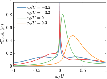
Figure 4: The normalized spectral function $\pi\Gamma_{L}A_{L}(\omega)$ of the left subsystem calculated for various orbital energy $\varepsilon_{d}$, as indicated. The other parameters are the same as in Fig. 2.

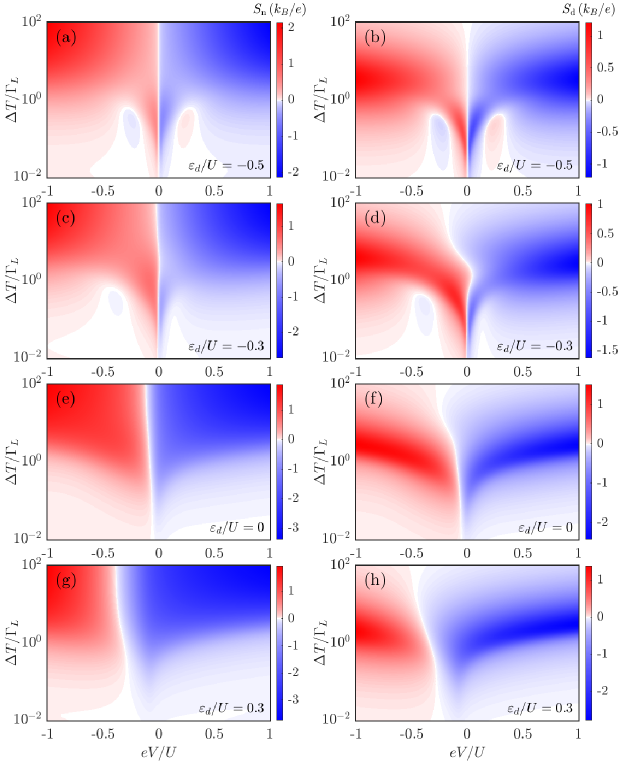
Figure 5: (Left column) The nonequilbrium Seebeck coefficient $S_{\rm n}$ and (right column) the differential Seebeck coefficient $S_{\rm d}$ calculated as a function of the temperature gradient $\Delta T$ and the applied bias voltage $V$. (a) and (b) present the case of the particle-hole symmetry point $\varepsilon_{d}/U=-0.5$, (c) and (d) show the local moment regime with $\varepsilon_{d}/U=-0.3$, (e) and (f) display the resonant tunneling regime $\varepsilon_{d}/U=0$, whereas (g) and (h) present the empty orbital regime with $\varepsilon_{d}/U=0.3$.

Figure 6: The temperature gradient dependence of (left column) the nonequilibrium and (right column) the differential Seebeck coefficients for different values of the bias voltage applied to the system, as indicated. (a) and (b) present the case of $\varepsilon_{d}/U=-0.5$, while (c) and (d) display the case of $\varepsilon_{d}/U=-0.3$, respectively. This figure corresponds to the vertical cross-sections of Figs. 5(a)-(d).

The fact that $S_{\rm n}$ and $S_{\rm d}$ for $V\rightarrow 0$ and $\Delta T\rightarrow 0$ should recover the linear response thermopower $S_{\rm lin}$ justifies the comparison of $S_{\rm n}(\Delta T)$ and $S_{\rm d}(\Delta T)$ to $S_{\rm lin}(T)$. The cross-sections in Figs. 3(b) and (d) compare $S_{\rm n}$ and $S_{\rm d}$ as a function of $\varepsilon_{d}$ and $\Delta T$, respectively, along with the linear response thermopower $S_{\rm lin}$ calculated for the system with global temperature $T=\Delta T$, denoted as colored circles.

We note that the dependence of the differential Seebeck coefficient $S_{\rm d}$ over the temperature gradient $\Delta T$ shows good agreement with the behavior of the linear response Seebeck effect $S_{\rm lin}$ with the global temperature $T$ even at large temperature gradients. This is not surprising due to the fact that for $\mu_{\rm L}=0$ and $T_{\rm L}=0$, Eq. (11) gives a formally similar expression for $S_{\rm lin}(T)$ and $S_{\rm d}(\Delta T)$. It is also interesting to note that, although $S_{\rm n}$ deviates from this behavior at large temperatures, the $S_{\rm n}(\Delta T)$ dependence when rescaled by 2 in $\Delta T$, i.e. $S_{\rm n}(2\Delta T)$ [see the dashed lines in Fig. 3(d)], agrees well with the linear response behavior for low values of $\Delta T$, see Fig. 3(d).

To further understand the behavior of the Seebeck coefficients in Fig. 3, one can separately focus on the three regimes. Since for $V\to 0$ thermopower is an odd function across the particle-hole symmetry point, we pick representative values of $\varepsilon_{d}$ for $\varepsilon_{d}>-U/2$. In the local moment regime, see the case of $\varepsilon_{d}/U=-0.3$ in Fig. 3(d), $S_{\rm n}$ first starts decreasing with raising $\Delta T$ until $\Delta T\approx T_{K}$ and then it increases to reach a sign change occurring around $\Delta T/\Gamma_{L}\approx 1$. Further increase of $\Delta T$ however gives rise to another sign change and the thermopower becomes again positive for large temperature gradients. Such behavior is consistent with the linear-response considerations of Kondo-correlated systems [9, 17]. Here, however, we demonstrate that it extends to nonlinear response regime. The above-described behavior is absent when the orbital level is tuned out of the Kondo regime. For resonant conditions, i.e. $\varepsilon_{d}=0$, $S_{\rm n}$ grows only in a monotonic fashion with increasing $\Delta T$. The same can be observed for the empty orbital case ($\varepsilon_{d}/U=0.3$), but now the value of $S_{\rm n}$ gets enhanced for $\Delta T/\Gamma_{L}\gtrsim 1$, compared to the case of $\varepsilon_{d}=0$.

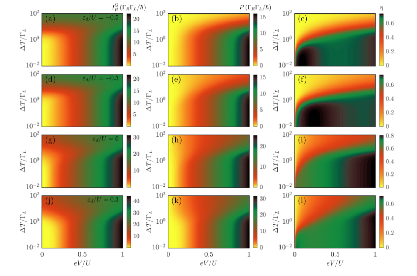
Figure 7: (left column) The heat current $I_{R}^{Q}$, (middle column) the power $P\equiv I_{R}^{Q}-I_{L}^{Q}$, as well as (right column) the thermoelectric efficiency $\eta$ calculated as a function of the applied bias voltage $V$ and the temperature gradient $\Delta T$ for different values of orbital energy $\varepsilon_{d}$. The first row is determined for $\varepsilon_{d}/U=-0.5$, the second one for $\varepsilon_{d}/U=-0.3$, the third row is for $\varepsilon_{d}=0$, while the last one is calculated for $\varepsilon_{d}/U=0.3$. The other parameters are the same as in Fig. 2.

III.2.2 Thermopower for finite temperature gradient and bias voltage

After analyzing the influence of the nonlinear temperature gradient on the Seebeck coefficient at linear potential bias, we will now proceed with the examination of the thermopower in the presence of both finite bias voltage and temperature gradient. Figure 5 presents the nonequilibrium and differential Seebeck coefficients calculated for finite potential and temperature gradients for different values of the orbital level energy, as indicated.

Let us first focus on the case when at low voltages the system is in the local moment regime. This is presented in Figs. 5(a,b) for the particle-hole symmetry point ($\varepsilon_{d}/U=-0.5$), and in Figs. 5(c,d) when detuned out of the symmetry point ($\varepsilon_{d}/U=-0.3$). From the linear response studies, one can expect the thermopower at the particle-hole symmetry point to vanish, since $S$ can be related to the slope of the spectral function $\frac{\partial A_{L}(\omega)}{\partial(\omega)}$ around the Fermi energy of the left lead in our case. In our system, where the potential bias is applied asymmetrically (only on the right lead), we are essentially shifting the system out of the symmetry point with an applied bias potential. This results in a non-zero Seebeck effect for a finite potential bias even in the case of $\varepsilon_{d}=-U/2$, see the first row of Fig. 5. As can be seen, in the nonlinear response regime for $\varepsilon_{d}=-U/2$, both $S_{\rm n}$ and $S_{\rm d}$ become finite and are odd functions of the applied bias voltage. More specifically, we observe positive Seebeck coefficients for negative applied bias voltage and vice versa. When the temperature gradient is of the order of the Kondo temperature, there is a new region of sign change present in the thermopower when the potential bias is between the range $0.2\lesssim|eV/U|\lesssim 0.4$, i.e. the system is in the Coulomb blockade. This sign change, visible in both $S_{\rm n}$ and $S_{\rm d}$ at nonequilibrium settings, is due to the Kondo correlations. The sign changes of the differential Seebeck coefficient $S_{\rm d}(V)$ at low temperature gradient $\Delta T$ can be inferred directly from the slope of the spectral function. From Eq. (2), when $|eV|\gg\Delta T$, the thermal response $\frac{\partial I}{\partial\Delta T}$ does not change considerably, resulting in the sign of $S_{\rm d}$ to be entirely dependent on $G=\frac{\partial I}{\partial V}$, cf. Eq. (8). This mandates the sign of $S_{\rm d}$ to roughly follow the sign of the function $f(eV)=-(\frac{\partial A_{L}(\omega=eV)}{\partial\omega})^{-1}$. When the bias voltage increases further, the Fermi levels of the leads are too far apart to show any effect of Kondo correlations on transport. In other words, the system leaves the Coulomb blockade regime for $|eV/U|\gtrsim 0.5$. For the case of the orbital level detuned out of the p-h symmetry point, we observe that the dependence of thermopower becomes generally asymmetric with respect to the bias reversal. For $\varepsilon_{d}/U=-0.3$, the sign changes corresponding to the Kondo correlations are present only for negative bias voltage, where the regime of sign change moves to slightly more negative bias voltage, $-0.5\lesssim eV/U\lesssim-0.25$. Interestingly, there is a new sign change, seen mostly in the temperature dependence of $S_{\rm d}$ for small positive bias voltages, which develops around $\Delta T/\Gamma_{L}\approx 1$, see Fig. 5(d).

All the features discussed in the case when at low voltages the system is in the local moment regime are nicely exemplified in Fig. 6, which presents the relevant vertical cross-sections of Fig. 5. One can clearly see the development of a finite Seebeck effect with increasing the potential bias in the case of $\varepsilon_{d}/U=-0.5$, where a small sign change for $|eV|/U=0.3$ can be observed. Note also the symmetry with respect to the bias reversal. On the other hand, even larger and generally nonzero for any value of $V$ thermopower develops for $\varepsilon_{d}/U=-0.3$. Here, one can explicitly see the sign changes of both $S_{\rm n}$ and $S_{\rm d}$ in the low bias voltage regime, which then disappear when the bias voltage increases.

The case when at equilibrium the orbital level is outside the local moment regime is presented in Figs. 5(e,f) for $\varepsilon_{d}=0$ and in Figs. 5(g,h) for the empty orbital case $\varepsilon_{d}/U=0.3$. Now, we generally observe only one sign change visible in the Seebeck coefficients $S_{\rm n}$ and $S_{\rm d}$ as a function of the applied bias voltage. Moreover, there is also a sign change as a function of thermal gradient for selected value of $V$. In the case of $\varepsilon_{d}/U=0$, the sign change is close to zero voltage and the offset from $V=0$ can be explained by renormalization of the orbital level by charge fluctuations with the strongly coupled lead, which give rise to a resonance in $A_{L}(\omega)$ slightly shifted with respect to the Fermi energy, cf. Fig. 4. When the potential bias $V$ is positive, both Seebeck coefficients, $S_{\rm n}$ and $S_{\rm d}$, are found to be negative. Moreover, in the regions of negative voltages, the magnitude of voltage required to change the sign of the thermopower increases with raising the temperature gradient. We observe a similar behavior in the case of $\varepsilon_{d}/U=0.3$, but the sign change of the Seebeck effect with respect to the potential bias is offset by the value of $\varepsilon_{d}$ in the negative voltage direction, see the last row of Fig. 5.

III.3 Nonequilibrium heat current and the thermoelectric efficiency

Figure 7 presents the bias voltage and temperature gradient dependence of the heat current $I_{R}^{Q}$ associated with the right subsystem, the power $P$ generated by the device together with the thermoelectric efficiency, cf. Eq. (13), calculated for several values of the dot level position, as indicated. First of all, we note the general tendency to increase the heat current by raising $V$ or $\Delta T$, which is irrespective of the level position $\varepsilon_{d}$. Moreover, for large bias voltages, there is a saturation and a slight decrease of $I_{R}^{Q}$ with increasing $\Delta T$. The same can be observed for the power generated by this device. Up to $eV\sim U/2$, the increase of the temperature gradient gives rise to an enhancement of the power. However, for larger voltages, there is a nonmonotonic dependence of $P$ with respect to $\Delta T$. The efficiency of the system is presented in the right column of 7. One can clearly identify an optimal choice of both $\Delta T$ and $V$, for which $\eta$ becomes maximized. The parameter space with maximum $\eta$ strongly depends on the transport regime. Interestingly, in the local moment regime, see Figs. 7(c) and (f), the maximum efficiency is obtained just around the Kondo regime. On the other hand, out of the Coulomb blockade and Kondo regime, the maximum efficiency occurs for larger voltages $eV/U\gtrsim 0.5$, see the case of $\varepsilon_{d}=0$ and $\varepsilon_{d}/U=0.3$ in Figs. 7(i) and (l). We also note that the Carnot efficiency for our system where $T_{L}\to 0$ is $\eta_{C}=1$. Consequently, we predict that the efficiency of the considered device can reach up to $\eta/\eta_{C}\approx 0.8$, depending on the transport regime.

III.4 Realistic junction

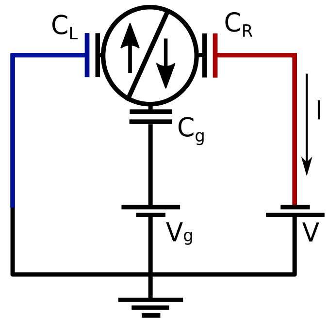
Figure 8: The schematic shows an equivalent electrical circuit diagram for the asymmetrically coupled molecular junction along with the implementation of the bias potential $V$ and the gate potential $V_{g}$. The capacitances associated with the left, right and the gate electrodes are represented as $C_{L}$, $C_{R}$ and $C_{g}$, respectively.

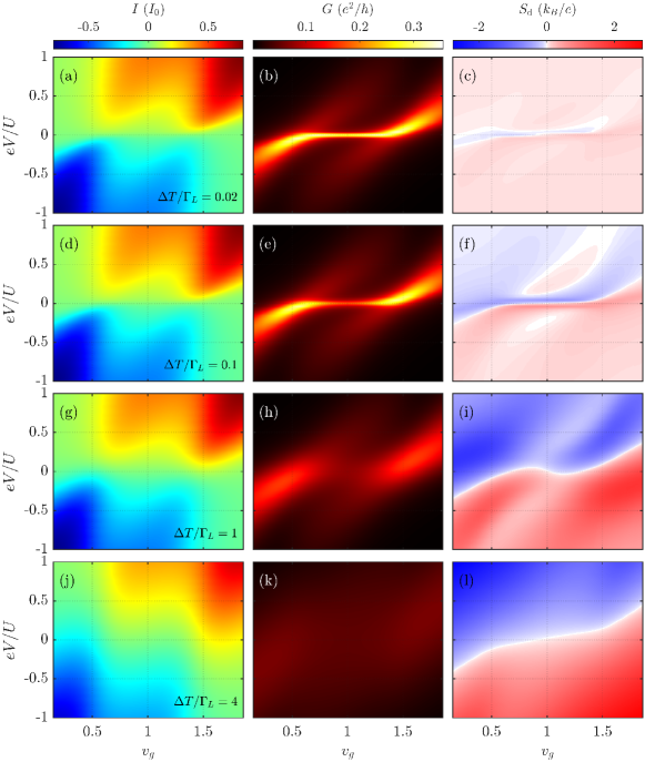
Figure 9: (First column) The current $I$ in units of $I_{0}=2e\Gamma_{R}/\hbar$, (second column) the differential conductance $G$ and (third column) the differential Seebeck coefficient $S_{\rm d}$ calculated as a function of the applied bias voltage $V$ and the effective gate voltage $v_{g}$. For the capacitances we assume $C_{L}/C_{R}=2$ and $C_{g}/C_{R}=0.1$ and the other parameters are the same as in Fig. 2. Each row corresponds to different temperature gradient $\Delta T$, as indicated.

To make the discussion of nonequilibrium thermopower more appealing to experimental realizations, in this section we relax the condition of voltage-independent orbital level and include the voltage drops assuming realistic junction parameters. An electrical circuit diagram of the considered system is shown in Fig. 8. The tunnel junctions are characterized by the capacitances $C_{L}$ and $C_{R}$, and the gate capacitance is denoted by $C_{g}$ with gate voltage $V_{g}$. The formula for the current flowing through such system can be written as

$$I(V,\Delta T) = -\frac{2e\Gamma_{R}}{\hbar}\!\int_{-\infty}^{\infty}\!d\omega A_{L}(\omega,v_{g}-v)\times$$ (14)

$$\left[f_{L}(\omega)-f_{R}(\omega-eV)\right],$$

where $v_{g}=C_{g}V_{g}/e$ and $v=VC_{R}/e$ are the dimensionless gate and bias voltage drops [33]. For the junction capacitances, we assume $C_{L}/C_{R}=2$ and $C_{g}/C_{R}=0.1$, while the charging energy $E_{C}=e^{2}/2C$, with $C=C_{L}+C_{R}+C_{g}$, is equal to $E_{C}=U/2$.

The current, differential conductance and differential Seebeck effect as a function of the bias voltage $V$ and the dimensionless gate voltage $v_{g}$ calculated for different temperature gradients are shown in Fig. 9. At low bias voltages, $v_{g}$ sets the corresponding transport regimes: $v_{g}\lesssim 0.5$ ($v_{g}\gtrsim 1.5$) defines the empty (fully occupied) orbital regime, whereas the local moment regime is realized for $0.5\lesssim v_{g}\lesssim 1.5$. Let us first analyze the case of the lowest temperature gradient, shown in the first row of Fig. 9, which corresponds to the situation when $\Delta T<T_{K}$. In Fig. 9(a) one can see a clear Coulomb diamond structure. On the other hand, the differential conductance exhibits then a pronounced zero-bias Kondo peak in the singly occupied orbital regime, i.e. $0.5\lesssim v_{g}\lesssim 1.5$. Note, that the behavior of the differential conductance is typical for tunnel junctions with asymmetric couplings to the contacts. Alternatively, one could also think of an adatom probed by a scanning tunneling microscope tip, which would correspond to a weakly coupled lead. At low temperatures, the differential thermopower is generally relatively small, however, one can still recognize sign change at low bias voltage regime, see Fig. 9(c).

When the thermal gradient becomes comparable to the Kondo temperature, the thermal response gets enhanced. This is presented in the second row of Fig. 9. Although the current is hardly affected, the differential conductance shows a suppression of the Kondo resonance at zero bias voltage. Moreover, the differential Seebeck coefficient is increased at low bias voltages. In addition, in the Kondo regime one can clearly see a sign change of $S_{\rm d}$ as a function of positive bias voltage.

With increasing the temperature gradient even more, see the case of $\Delta T/\Gamma_{L}=1$ in Fig. 9, the Coulomb diamond structure becomes smeared, and so does the conductance, which now only shows broad resonances due to resonant tunneling processes. The differential thermopower, on the other hand, is now much enlarged and it generally displays two regimes of either negative or positive values. Note, however, that the wavy line along which $S_{\rm d}$ changes sign strongly depends on both $V$ and $v_{g}$, which is due to the voltage dependence of the orbital level. Finally, for larger temperature gradients, $\Delta T/\Gamma_{L}>1$, see the last row of Fig. 9, most of the features are smeared. The differential conductance is suppressed by the thermal fluctuations, whereas the differential Seebeck effect again shows two regimes with different signs, but now separated by a line that monotonously depends on $v_{g}$.

IV Summary

In this paper we have studied the nonequilibrium thermoelectric transport properties of a molecular junction comprising a single-orbital molecule (or a quantum dot) asymmetrically attached to external electrodes. For such setup, we have determined the nonequilibrium electric and heat currents flowing through the system by using the perturbation theory with respect to the weakly coupled contact, while the strongly coupled subsystem was solved by using the numerical renormalization group method. This allowed us to accurately take into account the electronic correlations that result in the development of the Kondo effect between the molecule and strongly coupled lead. In particular, we have determined the temperature gradient and bias voltage dependence of the nonlinear $S_{\rm n}$ and differential $S_{\rm d}$ Seebeck coefficients. First, we have performed the calculations assuming that the orbital level position is independent of the applied bias. Then, assuming realistic junction parameters, we have also considered the case when this condition is relaxed. In particular, we have shown that both $S_{\rm n}$ and $S_{\rm d}$ exhibit sign changes at nonequilibrium conditions, which are due to Kondo correlations. Up to now, such Kondo-related sign changes have been mostly observed in the linear response regime [9]. In addition, we have also determined the nonequilibrium heat currents, the power generated by the device, when it works as a heat engine, and the corresponding thermoelectric efficiency. We have found transport regimes characterized by a considerable efficiency of up to $80\%$ of the Carnot efficiency. We believe that our results shed new light on the thermopower of strongly-correlated molecular junctions in out-of-equilibrium settings and will foster further efforts in the examination of such systems.