Don’t Lie to Me: Avoiding Malicious Explanations with STEALTH

Abstract

STEALTH is a method for using some AI-generated model, without suffering from malicious attacks (i.e. lying) or associated unfairness issues. After recursively bi-clustering the data, STEALTH system asks the AI model a limited number of queries about class labels. STEALTH asks so few queries (1 per data cluster) that malicious algorithms (a) cannot detect its operation, nor (b) know when to lie.

In order to support open science practices, all our scripts and data are on-line at https://github.com/laurensalvarez/STEALTH.

I Introduction

Within the current AI industry, there are many available models– not all of which can be inspected. “Model stores” are cloud-based services that charge a fee to use models hidden away behind a firewall (e.g. AWS market-place [1] and the Wolfram neural net repository[2]). Adams et al. [3] discusses model stores (also known as “machine learning as a service”[4]), and warns that these models are often low quality (e.g. if it comes from a hastily constructed prototype from a GitHub repository, dropped into a container, and then sold as a cloud-based service). Theoretically, software testing can defend us against low-quality models, but in practice, these models do not come with verification results nor detailed specifications– so standard testing methods are unsure what to test.

An alternative to testing is explanation algorithms that offer a high-level summary of a model. Unfortunately, the more we learn about explanations, the better we get at making misleading explanations. As we shall see:     The more a model is queried, the better it can mislead. For example, Slack et al.’s lying algorithm[5] (discussed below) knows how to detect “explanation-oriented” queries, and can then switch to models which, by design, disguise biases, or unfairness, against marginalized groups (e.g. by gender, race, age, or other identifiers).

Slack et al.’s results are particularly troubling. An alarming number of commercially deployed models have discriminatory properties[6, 7]. For example, the (in)famous COMPAS model (described in Table IV) decides the likelihood of a criminal defendant reoffending. The model suffers from alarmingly high false positive rates for Black defendants than White defendants. Noble’s book Algorithms of Oppression offers a long list of other models with discriminatory properties[6]. Clearly, before we can trust models from the cloud, we need ways to assess their bias without being misled by malicious algorithms.

This article reasons as follows. If too many queries are the problem, then perhaps the solution is:                           Ask fewer queries. To test this idea, we built a new algorithm called STEALTH which recursively bi-clusters $N$ examples, down to leaves of size $\sqrt{N}$. A model is then queried with 1 example per leaf. These queries generate “labels”; i.e. decisions about each $\sqrt{N}$ example, and are used to build a surrogate model which can be used for predictions and explanations. The key point here is since STEALTH makes few queries, malicious algorithms can not detect its operation. Hence, they never know when to lie. Also, since we use our surrogate for explanations, those explanations cannot be misled by a malicious model.

However, this assumes the surrogate (learned from very few samples) can mimic the important properties of the original model(learned from more data). To test that, our research questions ask what is gained and lost by reasoning over such a small $\sqrt{N}$ sample of the data:

RQ1: Does our method prevent lying? When querying Slack et al.’s lying algorithm, we found while the original model can lie, lying fails in our surrogates.

RQ2: Does the surrogate model perform as well as the original model? Much to our surprise, in the usual case, STEALTH’s surrogates performed as well as or better than the original (MODEL1), measured in terms of both predictive performance and fairness.

RQ3: How does STEALTH compare against other bias mitigation algorithms? Another reason to use STEALTH is its fairness properties are competitive to those generated via state-of-the-art bias mitigation methods such as Fair-Smote[7], MAAT[8], and FairMASK[9].

II Background (How to Lie)

Figure 1.A shows the Local Interpretable Model-Agnostic Explanations (LIME) algorithm[10] that samples thousands of instances uniformly at random near an example point, then builds a class of linear models from the generated sample data. Using its models, LIME can explain what features influence the classification of a particular instance.

LIME’s explanations look like Figure 1.B. Note that, in the figure, the Age feature is most influential. By running LIME on all the test instances, it is possible to collect the most influential features; i.e. the attributes that are found as being most influential for the test set.

An interesting result seen in the most influential feature set is that often most features are not influential. For example, in our study, we have ten data sets with dozens of attributes, but only a handful are ranked most influential. This indicates the most influential features are a useful way to summarize the differences between explanations generated via different methods. Given the two most influential sets $A,B$ a Jaccard coefficient is computed between (0,1) meaning (zero, total) similarities in the explanations, respectively:

$$\mathit{jaccard}(A,B)=\frac{|A\bigcap B|}{|A\bigcup B|}$$ (1)

To build a lying algorithm, we note that, in Figure 1.C, many of the red dots (showing LIME’s generated samples) are at different locations to the raw data (blue dots). Slack et al.[5] built a classifier to recognize when many of these red dots appear as input to the model. This meant they could distinguish (a) queries-about-explanation from (b) normal-queries seen in day-to-day operation. Hence they could hide any discriminatory properties by offering a lying model to queries-about-explanation and a second model to normal-queries.

To build their liar, Slack et al. trained an out-of-distribution (OOD) model using similar mutations to LIME and used this OOD detector to produce different classifications using the protected attributes. These are special attributes that divide data into two, privileged & unprivileged, groups (e.g. male & female; young & old). Thus, by training a model to recognize OOD data and in-distribution data, it is possible to hide discriminatory classifications against unprivileged groups, and mislead explanations.

Figure 1.A: LIME samples around the boundary to find the delta between blue and red classes. From[10].

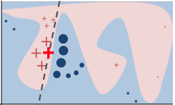
Figure 1.B: Feature importance as assessed by LIME. A positive weight means the feature encourages the classifier to predict the instance as a positive and vice versa for the negative weight. Larger weights indicate greater feature importance.

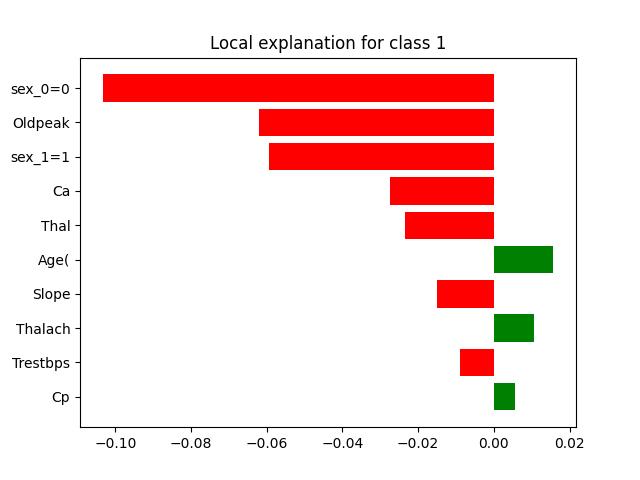
Figure 1.C: Blue/red = original/invented data [5].

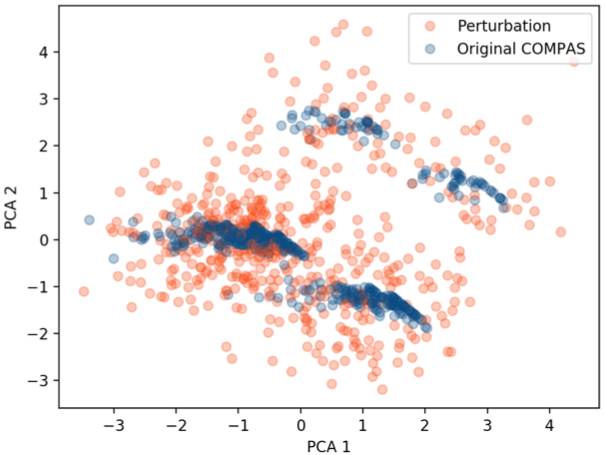
Figure 1: About LIME.

The problems raised by Slack et al.[5] are widely explored– see Table I. In that table, STEALTH’s use of limited domain data as samples is novel. Are such small samples of domain data relevant? We claim, without controversy, that for a model store to profit, consumers must want to use it, and know their own domain data they wish to label. For example, a doctor could have many records of patients and want to query a model to obtain a label of “high risk” or “low risk” of an imminent heart attack. More formally, given a data set with independent attributes $X$ and dependent classes $Y$, our approach assumes access to many $x_{i}$ rather than other researchers who assume no access to $x_{i}$ or $y_{i}$ and instead use randomly generated $x_{i}$ values. The starting point for this research was the realization that often model users do have $x_{i}$ data, but not $y_{i}$ labels. Our goal is to learn $Y=\mathit{MODEL1}(X)$ under the following “STEALTH assumptions”:

• We have domain data for $x_{i}$, but not $y_{i}$

• We can obtain $y_{i}$ values by querying a model MODEL2

• MODEL2 may be malicious

• To avoid being misled, we must limit the number of $y_{i}$ queries

Given the STEALTH assumptions, we first cluster our data on the $x_{i}$ values and then make one $y_{i}$ query per cluster. Using the few $x_{i}$ and associated $y_{i}$ labels, we build a surrogate model. The limited $y_{i}$ queries would add very few red points to Figure 1, because the points are domain data samples and would be identical to the blue dots making our STEALTH approach inherently undetectable.

TABLE I: Related Work

If the problem is that, in Figure 1.C, the red dots are different to the blue then one solution is to make LIME’s perturbations more realistic by adjusting sampling distributions [1], or better neighborhood calculations [2,3,4,5]. Other approaches improve LIME by making it more robust and less vulnerable to attacks [4,5], or creating better detection defenses [6,7] This is a very active area of research see [8-12] where prior work is rapidly assessed, improved, or refuted by subsequent work. We have three comments on that related work. Firstly, some of that work makes restrictive assumptions about the data. For example, Ji et al. [1] rely on parametric assumptions such as the data and model output conforming to a normal distribution. While such assumptions might be true, they cannot be checked in the black-box case. STEALTH, on the other hand, is a non-parametric instance-based approach that makes no assumptions of normality. Secondly, some works assume complexity when that may not be the best engineering decision for all domains. As shown by the results of this paper, methods that require 1000s of random samples (e.g. LIME) and which assume very high dimensional data (e.g. generative adversarial networks [4,5]) are not appropriate in all domains. Thirdly, the above work does not take full advantage of non-generated data. Model store consumers must have a supply of their own domain data they wish to label. We can use that to great effect as discussed in the main text. Related work citations: 1. D. Ji, P. Smyth, and M. Steyvers, “Can i trust my fairness metric? assessing fairness with unlabeled data and bayesian inference,” in NeurIPS’20. 2. D. Vreˇs and M. R. ˇSikonja, “Better sampling in explanation methods can prevent dieselgate-like deception,” arXiv:2101.11702, 2021. 3. Y. Jia, J. Bailey, et al. “Improving the quality of explanations with local embedding perturbations,” in KDD 2019, pp. 875–884. 4. S. Saito, E. Chua, N. Capel, and R. Hu, “Improving lime robustness with smarter locality sampling,” arXiv preprint arXiv:2006.12302, 2020. 5. A. Saini and R. Prasad, “Select wisely and explain: Active learning and probabilistic local post-hoc explainability,” AAAI/ACM Conference on AI, Ethics, and Society, 2022, pp. 599–608. 6. Z. Carmichael and W. J. Scheirer, “Unfooling perturbation-based post hoc explainers,” arXiv preprint arXiv:2205.14772, 2022. 7. J. Schneider, J. Handali, M. Vlachos, and C. Meske, “Deceptive ai explanations: Creation and detection,” arXiv preprint arXiv:2001.07641, 2020 8. Slack, D., Hilgard, A., Lakkaraju, H., & Singh, S., ”Counterfactual explanations can be manipulated,” in NeurIPS ’21 9. Wilking, R., Jakobs, M., & Morik, K., ”Fooling Perturbation-Based Explainability Methods,” In ECML/PKDD ’22. 10. Molnar, C., König, G., Herbinger, J., Freiesleben, T., Dandl, S., Scholbeck, C. A., … & Bischl, B., ”General pitfalls of model-agnostic interpretation methods for machine learning models,”. xxAI - Beyond Explainable AI. 2020. 11. Maratea, A., & Ferone, A., ”Pitfalls of local explainability in complex black-box models,” In WILF. 2021. 12. Covert, I., et al. ”Explaining by Removing: A Unified Framework for Model Explanation,” J. Mach. Learn. Res. 22 (2021): 209-1.

TABLE II: Inside STEALTH: The core of STEALTH is steps 2-5. Step 1,6, and 7 are added for evaluation.

0. Data Preparation The available data is divided 40:40:20 into a Train1:Train2:Test split. The test set is used as a set of hold-out examples in steps 1, 6, and 7. The Train1 set is used to build MODEL1 that we are trying to understand (and which might be managed by a malicious model manager). STEALTH does not use the class attribute labels in Train2 since its mission is to extract these from the limited number of queries to MODEL1 learned from Train1. Hence, for these experiments, all the class labels in Train2 are initially set to null.

1. Baseline generation: Build MODEL1 (also known as the original model) using 40% training data. In terms of our domain modeling, MODEL1 is the model hiding behind a firewall. Using MODEL1 and the 20% hold-out test data, we can collect baseline values for all the metrics of Table III.

2. Clustering: A clustering algorithm recursively bi-cluster Train2 data to leaves of size $\sqrt{N}$. We use Figure 2’s recursive bi-clustering method. Nair et al. report that this method is fast and useful for finding a good spread of examples across data[11].

3. Sampling: After that, we need a leaf sampling algorithm to select $m$ examples per leaf. Here, we selected $m=1$ items at random. While STEALTH works at $m=1$, other algorithms such as MAAT[8] seem to fail for such small data sets, and for some test cases, we cannot validate them with respect to prior work.

4. Labeling: A labeling algorithm must then assign labels to $\sqrt{N}$ selected examples. For that purpose, we query MODEL1.

5. Surrogate Creation: Some model creation algorithm must build a surrogate model. Here again, we used a random forest to build MODEL2 (also known as the surrogate model) using the data associated with the $\sqrt{N}$ labels.

6. Collect Performance Scores: Here, the surrogate MODEL2 is applied to the 20% hold-out test data to generate the Table III performance scores. These values are compared to the baseline values seen in step 1.

7. Collect Explanation Scores: Here, we gather the most influential attributes of (b1) MODEL1 and (b2) MODEL2 using LIME, and compare them using Equation 1.

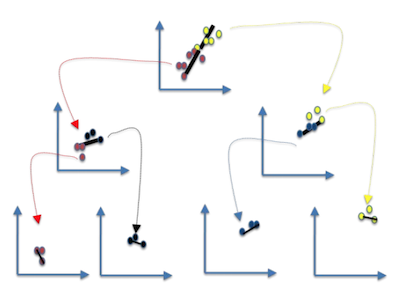
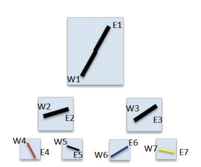
Figure 2: STEALTH partitions $x$ values using the random projections. Nair et al. report that this method is fast and is useful for generating a good spread of examples across a data set [10].

NOTES: This recursive bi-clustering method finds two distant points $E$ (east) and $W$ (west). Using $c=\mathit{dist}(E,W)$ then all other examples have distances $a,b$ to $E,W$, respectively and distance $x=(a^{2}+c^{2}-b^{2})/(2c)$ on a line from $E$ to $W$. By splitting data on median $x$, the examples can be then bi-clustered (and so on, recursively, see Figure 2b).

Figure 2a.

Figure 2b.

TABLE III: Evaluation metrics. In this table, TP, TN, FP, FN are the true/false positive/negative rates seen in binary classification. The definition for True Positive Rates (TPR) is TP$/$(TP $+$ FN) and False Positive Rates (FPR) is FP$/$(FP $+$ TN).

Performance Metric	Fairness Metric
Accuracy = (TP$+$TN)$/$(TP$+$TN$+$FP$+$FN)	Average Odds Difference (AOD): Average of difference in False Positive Rates(FPR) and True Positive Rates(TPR) for unprivileged and privileged groups. $AOD$ $=$ (($FPR_{U}$-$FPR_{P}$) + ($TPR_{U}$-$TPR_{P}$))$/$ 2
False alarm = FP/(FP+TN)	Equal Opportunity Difference (EOD): Difference of True Positive Rates(TPR) for unprivileged and privileged groups. $EOD=TPR_{U}-TPR_{P}$
Recall = TP/(TP+FN)	Statisticl Parity Difference (SPD): Difference between probability of unprivileged group (protected attribute PA = 0) gets favorable prediction ($\hat{Y}=1$) & probability of privileged group (protected attribute PA = 1) gets favorable prediction ($\hat{Y}=1$). $SPD=P[\hat{Y}=1|PA=0]-P[\hat{Y}=1|PA=1]$
Precision = TP$/$(TP$+$FP)	Disparate Impact (DI): Similar to SPD but instead of the difference of probabilities, the ratio is measured. $DI=P[\hat{Y}=1|PA=0]/P[\hat{Y}=1|PA=1]$
F1 Score = 2 $\times$ (Precision $\times$ Recall)$/$(Precision $+$ Recall)

TABLE IV: Description of processed data sets including their domain usage, protected attributes, numerical features post-processing, and non-empty rows. STEALTH number of rows and median run-times in seconds over 20 repeats.

						Our
		Protected	Num	N	$\sqrt{N}$	runtimes
Data set	Domain	Attribute	Features	rows	rows	(secs)
Adult Census [1]	U.S. census information from 1994 to predict personal income	Sex, Race	7	45,522	512	58.89
Bank Marketing [2]	Marketing data of a Portuguese bank to predict term deposit	Age	7	30,488	512	54.54
Default Credit [3]	Customer information in Taiwan to predict default payment	Sex	24	30,000	512	94.98
Compas [4]	Criminal history of defendants to predict re-offending	Sex, Race	4	6,172	256	12.43
MEPS15 [5]	Surveys of household members and their medical providers	Race	41	4,870	128	2.00
Student [6]	Student performance to predict good grades	Sex	24	1,044	64	1.19
German Credit [7]	Personal information to predict good or bad credit	Sex	6	1,000	64	1.19
Diabetes [8]	Diagnostic measurements to predict diabetes	Age	8	768	64	1.14
Heart Health [9]	Patient information from Cleveland DB to predict heart disease	Age	13	297	58	1.11
Communities  [10]	Law enforcement information to predict violent crimes	racePctWhite	122	123	32	1.49

Data set citations:

1. ”Adult data set,” 1994. http://mlr.cs.umass.edu/ml/datasets/Adult

2. “Bank marketing,” 2017. https://www.kaggle.com/c/bank-marketing-uci

3. “Default of credit card clients data set,” 2016. https://archive.ics.uci.edu/ml/datasets/default+of+credit+card+clients

4. “Compas Analysis,” 2015. https://github.com/propublica/compas-analysis

5. “Medical expenditure panel survey,” 2015. https://meps.ahrq.gov/mepsweb/

6. “Student performance data set,” 2014. https://archive.ics.uci.edu/ml/datasets/Student$+$Performance

7. “German credit data set,” 2000. https://archive.ics.uci.edu/ml/datasets/Statlog+German+Credit+Data

8. U. M. Learning, “Pima indians diabetes database,” 2016. https://kaggle.com/uciml/pima-indians-diabetes-database

9. “Heart disease data set,” 2001. https://archive.ics.uci.edu/ml/datasets/Heart+Disease

10. M. Redmond, “Communities and crime unnormalized data set,” 2011. http://www.ics.uci.edu/mlearn/ML-Repository

III Methods

Table II describes the seven steps needed to run and evaluate STEALTH. To answer our research questions, we applied those steps, with and without Slack et al.’s lying algorithm [5]. The surrogate models built were assessed via their (a) LIME explanation properties (using Equation 1); (b) their predictive performance; and (b) their fairness using metrics that are widely applied in the literature (see Table III). Since we are exploring fairness, we also compare STEALTH to state-of-the-art bias reduction algorithms Fair-Smote[7], MAAT[8], and FairMASK[9].

ALGORITHMS: For this work, we tried various learners such as random forests, logistic regression, and a SVM with a radial basis function. It was observed that random forests generated better recalls, and thus, we focus on random forests for this work.

Table II uses several bias reduction methods. Chen et al.’s MAAT system[8] makes conclusions by balancing conclusions between two separate models (a performance model and a fairness. model). Chakraborty et al.’s Fair-SMOTE system[7] adjusts the training data by (a) removing training instances that change conclusions when protected attributes change; and (b) evening out the distributions of the protected attribute values. Chakraborty argues that these adjustments make it harder for any particular protected value to unduly affect the conclusion. Peng et al.’s FairMASK system[9] replaces protected attributes with new values learned from other independent attributes. Peng argues that this removed misleading latent correlations between attributes since the learned values tend to be average values (not outliers).

An important note to make about MAAT, Fair-SMOTE, and FairMASK is that all these methods require the analyst to pre-specify the protected attributes. STEALTH, on the other hand, operates without such knowledge. Despite this, as we will see, STEALTH achieves competitive levels of bias reduction to MAAT, Fair-SMOTE, and FairMASK.

DATA: The case studies in Table IV were selected since they appeared in prior explanation and fairness papers including Slack et al. [5]. In column three of Table IV, each protected attribute is listed.

STATISTICS: Eight of our data sets have one protected attribute while ADULT and COMPAS have two. Hence, we run 12 times, one for each data set and protected attribute. Each run is repeated 20 times, each time dividing the available data into 40% Train1, 40% Train2, and 20% Test. Since each run returns nine scores (one for each of the metrics of Table III), then generates 12*20*9=2160 scores.

For each data set and metric, we compared methods (using STEALTH or MAAT or FairSMOTE or FairMASK) against a baseline (running all data through random forests). Each method earns one more win, tie, or loss if it is statistically better, the same, or worse than the baseline (respectively). For that statistical test, we use a nonparametric test recommended by prior work on bias reduction; a Scott-Knot procedure using Cliffs Delta and a bootstrap test. For notes justifying and explaining those procedures, see[12, 13, 7, 8]. Note that for recall, precision, accuracy, and F1 larger numbers are better while for all other metrics such as false alarms, smaller numbers are better.

IV Results

RQ1: Does our method prevent lying?

Table V compares the explanations from Slack et al.’s lying algorithm and STEALTH’s Slack surrogate models. In Table V, we see that the Slack et al. entries are nearly all zero; i.e. explanations from STEALTH do not overlap with the lying algorithm’s explanations. This means that Slack’s algorithm cannot detect the operation of STEALTH, and so it never knows when to lie.

Generating different explanations, from the liar, could be achieved by selecting lucky random values. Happily, we can show that the explanations from STEALTH correspond to important influences within our models. Table V also shows us that explanations from STEALTH have a large overlap (median=59.5%) with the explanations from the original model, MODEL1.

In summary, to answer RQ1, we say STEALTH can defeat Slack et al.’s lying algorithm. This is not to say that STEALTH defeats all possible liars, and exploring our method in the context of other liars is a clear direction for future work.

For our methods, RQ1 is a positive result while many of the explanation overlaps reported in Table V are less than 100%. That is, between the original model and those made by STEALTH, there are differences measured in terms of which attributes are most influential. Happily, in conjunction with the results of RQ2, it suggests STEALTH’s models are preferable to the original, and arguably we should have more confidence in the most influential attributes, as reported by STEALTH.

TABLE V: RQ1 results: Jaccard coefficient (Equation 1) results comparing LIME’s first top-ranked features of MODEL1 (with the Baseline and the Slack et al. liar algorithm) to STEALTH’s first top-ranked features.

Data set	Slack_Jacc	Base_Jacc
student	0.08	0.25
meps	1	0.42
adult_r	0	0.50
adult_s	0	0.50
compas_s	0	0.57
		0.595 $\Longleftarrow$ median
diabetes	0.20	0.62
compas_r	0.0	0.67
default	0.07	0.68
bank	0.17	0.69
german	0	0.79

TABLE VI: RQ2 results: A method earns one win or tie or loss if it is statistically better, same, or worse(respectively) than the Figure 3 baseline (as assessed via Scott-Knot statistical tests that combine Cliffs Delta and a bootstrap). Note that for recall, precision, accuracy, and F1 larger numbers are better while for all other metrics such as false alarms, smaller numbers are better.

	Performance:				Fairness:
	(accuracy, recall, precision, F1, false alarm)				(AOD, EOD, SPD, DI)
Method	Wins	Loses	Ties	Wins + Ties	Wins	Loses	Ties	Wins + Ties
STEALTH	28	7	25	53 / 60	21	6	21	42 / 48
MAAT	34	17	9	43 / 60	31	7	10	41 / 48
Fair-SMOTE	27	17	16	43 / 60	28	6	14	42 / 48
FairMask	21	23	16	37 / 60	12	25	11	23 / 48

RQ2: Does the surrogate model perform as well as the original model?

It turns out that our method for avoiding liars does not lead to sub-optimal models. Table VI shows how often our method finds improvements over the baseline models. Note that there are many wins recorded in Table VI such as achieving numerous non-small, statistically significant improvements in performance and fairness compared to the baseline.

There are some losses reported in Table VI and to explain, we look at the raw values of the baseline models (shown in Figure 3). It is clear that in the original model, MODEL1, there are some weakly performing data sets. For example, in Figure 3, while ADULT has high accuracy, the baseline also suffers from very high false alarms (over 50%). This is relevant since, when we drill down into the losses of Table VI, we note that many of STEALTH’s losses arise in ADULT. That is to say, these losses seem to be less about drawbacks with STEALTH and rather drawbacks with random forests (for these data sets).

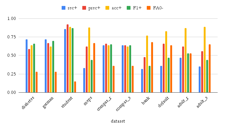
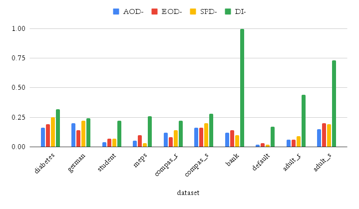
Figure 3.A: RQ2 results: performance reports median results for accuracy, recall, false alarm precision, F1. Figure 3.B: RQ2 results: fairness reports median results for EOD, AOD, SPD, DI

Figure 3: RQ2 Baseline, a non-malicious RF trained with all data, results on Table III metrics.

RQ3: Does the surrogate model enhance fairness? How does it compare to SOTA fairness mitigation methods?

Our summary of Table VI is that STEALTH is competitive with the current state-of-art, and even defeats some of those algorithms (e.g. FairMask). A case might be made that Fair-SMOTE and MAAT perform a little better since they have a few more wins (that said, the wins+ties are the same as STEALTH).

Hence, we see no reason to dismiss STEALTH based on the fairness of the models it creates, and given its superior performance scores, makes us recommend this algorithm.

Another reason to recommend STEALTH is that other bias reduction methods have to be directed to protect specific attributes. STEALTH, on the other hand, offers bias improvements without having to be directed. This is to say STEALTH could protect important attributes even if they were inadvertently overlooked.

V Discussion: Why Does it Work So Well?

By using a few examples, STEALTH runs “under the radar” and is undetected by Slack et al.’s lying algorithm. STEALTH makes very few ($\sqrt{N}$) in-distribution queries, which are undetectable by OOD attacks. Since STEALTH’s queries are undetectable, the liar cannot lie and returns honest results. Why do models built from just $\sqrt{N}$ examples have similar or better performance, and bias reduction properties? Perhaps this is for the same reason that semi-supervised reasoning[14] works so well. One of the relevant semi-supervised learner assumptions is the ”manifold assumption”, i.e. higher dimensional data can be approximated by a smaller set of most important attributes, without much loss of signal [14]. As evidence of our data having a lower dimensional manifold, recall from the above that in all the data sets used here, there were very few most influential attributes. When such smaller manifolds exist, data mining needs to only explore a small sample of the data set (provided the samples are spread across the data set using methods like, for example, Figure 2).

As to STEALTH’s success at reducing bias, we conjecture that STEALTH’s success results from a zealous use of design principles from Peng et al.’s FairMASK [9]. Peng et al. argue that FairMASK reduces bias by replacing minority outlier opinions with values that are better supported by more data. FairMASK does this by synthesizing replacement values for protected attributes from the other independent attributes. STEALTH, on the other hand, does this for all independent attributes since, in effect, its $\sqrt{N}$ examples are reports of average case effects within small data clusters. By averaging the data in this way, we smooth out the features including any outliers that may skew results unfairly.

(Technical aside: other fairness mitigation algorithms e,g, Fair-SMOTE, mitigate for unfairness by “blanding-out” attributes– i.e. by giving their values equal frequency in the training data. Our pre-experimental concern was that STEALTH operations on all attributes would bland-out everything, thus leading to a naive and poorly performing classifier. Yet, we realized it was the opposite of blanding-out. STEALTH builds a training set by clustering down to $\sqrt{N}$ and uses a random point near the centroids of the leaf clusters to build a surrogate. In so doing, STEALTH removes outlier signals and emphasizes the central tendencies within each of these $\sqrt{N}$ samples. Hence, we achieve the fairness results of Table VI by deleting spurious signals without having to explicitly annotate which attributes are protected.)

Based on the above, STEALTH can be called a fairness enhancing algorithm which we recommended over MAAT, Fair-SMOTE, and FairMASK. But also, we argue that there is another result here. An important feature of these results is they suggest a new view on the nature of explanation, discussion, and discrimination. The STEALTH results highlight a connection between “better, more honest explanations” and “reducing biased results” into something that we might call “trusted communication”. Are there other such “trusted communication” methods? Would they perform better than STEALTH? We do not know– but that would be a useful direction for future research.

References

- [1] A. Marketplace, “Machine learning & artificial intelligence,” 2019.
- [2] “Wolfram neural net repository.” [Online]. Available: https://resources.wolframcloud.com/NeuralNetRepository
- [3] M. Xiu, Z. Ming, Jiang, and B. Adams, “An exploratory study on machine learning model stores,” IEEE Software, 2021.
- [4] M. Ribeiro, K. Grolinger, and M. A. Capretz, “Mlaas: Machine learning as a service,” in 2015 IEEE 14th International Conference on Machine Learning and Applications (ICMLA). IEEE, 2015, pp. 896–902.
- [5] D. Slack, S. Hilgard, E. Jia, S. Singh, and H. Lakkaraju, “Fooling LIME and SHAP: Adversarial attacks on post hoc explanation methods,” in 3rd AAAI/ACM Conference on AI, Ethics, and Society, 2020.
- [6] S. U. Noble, Algorithms of Oppression. NYU Press, 2018. [Online]. Available: http://www.jstor.org/stable/j.ctt1pwt9w5.1
- [7] J. Chakraborty, S. Majumder, and T. Menzies, “Bias in machine learning software: why? how? what to do?” in Proceedings of the 29th ACM Joint Meeting on European Software Engineering Conference and Symposium on the Foundations of Software Engineering, 2021, pp. 429–440.
- [8] Z. Chen, J. Zhang, F. Sarro, and M. Harman, “Maat: A novel ensemble approach to addressing fairness and performance bugs for machine learning software,” in The ACM Joint European Software Engineering Conference and Symposium on the Foundations of Software Engineering (ESEC/FSE), 2022.
- [9] K. Peng, J. Chakraborty, and T. Menzies, “xfair: Better fairness via model-based rebalancing of protected attributes,” IEEE Trans SE, accepted, to appear, 2022. [Online]. Available: https://arxiv.org/abs/2110.01109
- [10] M. T. Ribeiro, S. Singh, and C. Guestrin, “”why should i trust you?”: Explaining the predictions of any classifier,” in Proceedings of the 22nd ACM SIGKDD International Conference on Knowledge Discovery and Data Mining, ser. KDD ’16. New York, NY, USA: Association for Computing Machinery, 2016, p. 1135–1144. [Online]. Available: https://doi.org/10.1145/2939672.2939778
- [11] J. Chen, V. Nair, R. Krishna, and T. Menzies, ““sampling” as a baseline optimizer for search-based software engineering,” IEEE Transactions on Software Engineering, vol. 45, no. 6, pp. 597–614, 2018.
- [12] M. R. Hess and J. D. Kromrey, “Robust confidence intervals for effect sizes: A comparative study of cohen’sd and cliff’s delta under non-normality and heterogeneous variances,” in annual meeting of the American Educational Research Association, vol. 1. Citeseer, 2004.
- [13] N. Mittas and L. Angelis, “Ranking and clustering software cost estimation models through a multiple comparisons algorithm,” IEEE Transactions on software engineering, vol. 39, no. 4, pp. 537–551, 2012.
- [14] O. Chapelle, B. Schölkopf, and A. Zien, Eds., Semi-Supervised Learning. The MIT Press, 2006. [Online]. Available: http://dblp.uni-trier.de/db/books/collections/CSZ2006.html