GePA*SE: Generalized Edge-Based Parallel A* for Slow Evaluations

Abstract

Parallel search algorithms have been shown to improve planning speed by harnessing the multithreading capability of modern processors. One such algorithm PA*SE achieves this by parallelizing state expansions, whereas another algorithm ePA*SE achieves this by effectively parallelizing edge evaluations. ePA*SE targets domains in which the action space comprises actions with expensive but similar evaluation times. However, in a number of robotics domains, the action space is heterogenous in the computational effort required to evaluate the cost of an action and its outcome. Motivated by this, we introduce GePA*SE: Generalized Edge-based Parallel A* for Slow Evaluations, which generalizes the key ideas of PA*SE and ePA*SE i.e. parallelization of state expansions and edge evaluations respectively. This extends its applicability to domains that have actions requiring varying computational effort to evaluate them. The open-source code for GePA*SE along with the baselines is available here:[Link anonymized]

Introduction

Graph search algorithms such as A* and its variants are widely used in robotics for planning problems which can be formulated as a shortest path problem on a graph (Kusnur et al. 2021; Mukherjee et al. 2021). Parallelized graph search algorithms have shown to be effective in robotics domains where action evaluation tends to be expensive. PA*SE (Phillips, Likhachev, and Koenig 2014) is an optimal parallel graph search algorithm that strategically parallelizes state expansions to speed up planning, without the need for state re-expansions. However, just like A*, PA*SE evaluates all edges at once for every state expansion in the same thread. In contrast, a parallelized planning algorithm ePA*SE (Edge-based Parallel A* for Slow Evaluations) (Mukherjee, Aine, and Likhachev 2022a) changes the basic unit of search from state expansions to edge expansions. This decouples the evaluation of edges from the expansion of their common parent state, giving the search the flexibility to figure out what edges need to be evaluated to solve the planning problem. In domains with expensive edges, ePA*SE achieves lower planning times and evaluates fewer edges than PA*SE. ePA*SE is efficient in domains where the action space is homogenous in computational effort i.e. all actions have similar evaluation times. In some domains, the action space can comprise a combination of cheap and expensive to evaluate actions. For example, in planning on manipulation lattices, the action space comprises static primitives generated offline, each of which moves a single joint and Adaptive Motion Primitives, which use an optimization-based IK solver to compute a valid goal configuration (based on the workspace goal) and then linearly interpolate from the expanded state to the goal  (Cohen, Chitta, and Likhachev 2014). The latter are generated online and are significantly more expensive to compute than the static primitives. In such domains, it is not efficient to delegate a new thread for every edge.

Motivated by these insights, we introduce GePA*SE which generalizes the key ideas in PA*SE and ePA*SE i.e. state expansions and edge evaluations respectively. We show that GePA*SE outperforms both PA*SE and ePA*SE in domains with heterogenous action spaces by employing a parallelization strategy that handles cheap edges similar to PA*SE and expensive edges similar to ePA*SE. Additionally, it uses a more efficient strategy to carry out edge independence checks for large graphs. While GePA*SE is optimal, its bounded suboptimal variant w-GePA*SE inherits the bounded suboptimality guarantees of wPA*SE and w-ePA*SE and achieves faster planning by employing an inflation factor on the heuristic. We evaluate w-GePA*SE in a 2D grid-world and a 7-DoF manipulation domain and demonstrate that it achieves lower planning times in both.

Related Work

Several approaches parallelize sampling-based planning algorithms in which multiple processes cooperatively build a PRM (Jacobs et al. 2012) or an RRT (Devaurs, Siméon, and Cortés 2011; Ichnowski and Alterovitz 2012; Jacobs et al. 2013) by sampling states in parallel. However, in many planning domains, sampling of states is not trivial. One such class of planning domains is simulator-in-the-loop planning, which uses a physics simulator to generate successors (Liang et al. 2021). Unless the state space is simple such that the sampling distribution can be scripted, there is no principled way to sample meaningful states that can be realized in simulation.

We focus on search-based planning which constructs the graph by recursively applying a set of actions from every state. A* can be trivially parallelized by generating successors in parallel when expanding a state. However, the performance improvement is bounded by the branching factor of the domain. Another approach is to expand states in parallel while allowing re-expansions to account for the fact that states may get expanded before they have the minimal cost (Irani and Shih 1986; Evett et al. 1995; Zhou and Zeng 2015). However, they may encounter an exponential number of re-expansions, especially if they employ a weighted heuristic. PA*SE (Phillips, Likhachev, and Koenig 2014) parallelly expands states at most once, in such a way that does not affect the bounds on the solution quality. ePA*SE (Mukherjee, Aine, and Likhachev 2022a) improves PA*SE by changing the basic unit of the search from state expansions to edge expansions and then parallelizing this search over edges. MPLP (Mukherjee, Aine, and Likhachev 2022b) achieves faster planning by running the search lazily and evaluating edges asynchronously in parallel, but relies on the assumption that a successor can be generated without evaluating the edge. There has also been some work on parallelizing A* on GPUs (Zhou and Zeng 2015; He et al. 2021). These algorithms have a fundamental limitation that stems from the SIMD (single-instruction-multiple-data) execution model of a GPU which limits their applicability to domains with simple actions that share the same code.

Method

Problem Formulation

Let a finite graph $G=(\mathcal{V},\mathcal{E})$ be defined as a set of vertices $\mathcal{V}$ and directed edges $\mathcal{E}$. Each vertex $v\in\mathcal{V}$ represents a state $\mathbf{s}$ in the state space of the domain $\mathcal{S}$. An edge $e\in\mathcal{E}$ connecting two vertices $v_{1}$ and $v_{2}$ in the graph represents an action $\mathbf{a}\in\mathcal{A}$ that takes the agent from corresponding state $\mathbf{s}_{1}$ to $\mathbf{s}_{2}$. The action space is split into subsets of cheap ($\mathcal{A}^{c}$) and expensive actions ($\mathcal{A}^{e}$) s.t. $\mathcal{A}^{c}\cup\mathcal{A}^{e}=\mathcal{A}$ and corresponding cheap ($\mathcal{E}^{c}$) and expensive edges ($\mathcal{E}^{e}$) s.t. $\mathcal{E}^{c}\cup\mathcal{E}^{e}=\mathcal{E}$. An edge $e$ can be represented as a pair $(\mathbf{s},\mathbf{a})$, where $\mathbf{s}$ is the state at which action $\mathbf{a}$ is executed. For an edge $e$, we will refer to the corresponding state and action as $e.\mathbf{s}$ and $e.\mathbf{a}$ respectively. $\mathbf{s}_{0}$ is the start state and $\mathcal{G}$ is the goal region. $c:\mathcal{E}\rightarrow[0,\infty]$ is the cost associated with an edge. $g(\mathbf{s})$ or g-value is the cost of the best path to $\mathbf{s}$ from $\mathbf{s}_{0}$ found by the algorithm so far. $h(\mathbf{s})$ is a consistent and therefore admissible heuristic (Russell 2010). A path $\pi$ is an ordered sequence of edges $e_{i=1}^{N}=(\mathbf{s},\mathbf{a})_{i=1}^{N}$, the cost of which is denoted as $c(\pi)=\sum_{i=1}^{N}c(e_{i})$. The objective is to find a path $\pi$ from $\mathbf{s}_{0}$ to a state in the goal region $\mathcal{G}$ with the optimal cost $c^{*}$. There is a computational budget of $N_{t}$ parallel threads available. There exists a pairwise heuristic function $h(\mathbf{s},\mathbf{s}^{\prime})$ that provides an estimate of the cost between any pair of states. It is forward-backward consistent (Phillips, Likhachev, and Koenig 2014) i.e. $h(\mathbf{s},\mathbf{s}^{\prime\prime})\leq h(\mathbf{s},\mathbf{s}^{\prime})+h(\mathbf{s}^{\prime},\mathbf{s}^{\prime\prime})~{}\forall~{}\mathbf{s},\mathbf{s}^{\prime},\mathbf{s}^{\prime\prime}$ and $h(\mathbf{s},\mathbf{s}^{\prime})\leq c^{*}(\mathbf{s},\mathbf{s}^{\prime})~{}\forall~{}\mathbf{s},\mathbf{s}^{\prime}$.

Algorithm

Similar to ePA*SE, GePA*SE searches over edges instead of states and exploits the notion of edge independence to parallelize this search. There are two key differences. First, GePA*SE handles cheap and expensive-to-evaluate edges differently. Second, it uses a more efficient independence check. In this section, we expand on these differences.

Algorithm 1 w-GePA*SE: Planning Loop

1:$terminate\leftarrow\text{False}$

2:procedure Plan

3:     $\forall\mathbf{s}\in G$, $\mathbf{s}.g\leftarrow\infty$, $n\_successors\_generated(s)=0$

4:     $\mathbf{s}_{0}.g\leftarrow 0$

5:     insert $(\mathbf{s}_{0},\mathbf{a^{d}})$ in OPEN $\triangleright$ Dummy edge from $\mathbf{s}_{0}$

6:     LOCK

7:     while $\textbf{not }terminate$ do

8:         if $\textit{OPEN}=\emptyset\textbf{ and }\textit{BE}=\emptyset$ then

9:              $terminate=\text{True}$

10:              UNLOCK

11:              $\textbf{return}{}~{}\emptyset$          

12:         remove an edge $(\mathbf{s},\mathbf{a})$ from OPEN that has the
          smallest $f((\mathbf{s},\mathbf{a}))$ among all states in OPEN that
          satisfy Equations 1 and 3

13:         if such an edge does not exist then

14:              UNLOCK

15:              wait until OPEN or BE change

16:              LOCK

17:              continue          

18:         if $\mathbf{s}\in\mathcal{G}$ then

19:              $terminate=\text{True}$

20:              UNLOCK

21:              return Backtrack($\mathbf{s}$)          

22:         UNLOCK

23:         while $(\mathbf{s},\mathbf{a})$ has not been assigned a thread do

24:              for $i=1:N_{t}$ do

25:                  if thread $i$ is available then

26:                       if thread $i$ has not been spawned then

27:                           Spawn $\textsc{EdgeExpandThread}(i)$                        

28:                       Assign $(\mathbf{s},\mathbf{a})$ to thread $i$                                          

29:         LOCK      

30:     $terminate=\text{True}$

31:     UNLOCK

Algorithm 2 w-GePA*SE: Edge Expansion

1:procedure ExpandEdgeThread($i$)

2:     while $\textbf{not }terminate$ do

3:         if thread $i$ has been assigned an edge $(\mathbf{s},\mathbf{a})$ then

4:              $\textsc{Expand}\left((\mathbf{s},\mathbf{a})\right)$               

5:procedure Expand($(\mathbf{s},\mathbf{a})$)

6:     if $\mathbf{a}=\mathbf{a^{d}}$ then

7:         insert $\mathbf{s}$ in BE with priority $f(\mathbf{s})$

8:         for $\mathbf{a}^{\prime}\in\mathcal{A}^{e}$ do

9:              $f\left((\mathbf{s}^{\prime},\mathbf{a})\right)=g(\mathbf{s})+wh(\mathbf{s})$

10:              insert $(\mathbf{s},\mathbf{a})$ in OPEN with $f\left((\mathbf{s}^{\prime},\mathbf{a})\right)$          

11:         UNLOCK

12:         for $\mathbf{a}^{\prime}\in\mathcal{A}^{c}$ do

13:              $\textsc{ExpandEdge}\left((\mathbf{s}^{\prime},\mathbf{a})\right)$          

14:         LOCK

15:     else

16:         $\textsc{ExpandEdge}\left((\mathbf{s},\mathbf{a})\right)$      

17:procedure ExpandEdge($(\mathbf{s},\mathbf{a})$)

18:     $\mathbf{s}^{\prime},c\left((\mathbf{s},\mathbf{a})\right)\leftarrow\textsc{GenerateSuccessor}\left((\mathbf{s},\mathbf{a})\right)$

19:     LOCK

20:     if $\mathbf{s}^{\prime}\notin\textit{CLOSED}\cup\textit{BE}$ and

21:            $g(\mathbf{s}^{\prime})>g(\mathbf{s})+c\left((\mathbf{s},\mathbf{a})\right)$ then

22:         $g(\mathbf{s}^{\prime})=g(\mathbf{s})+c\left((\mathbf{s},\mathbf{a})\right)$

23:         $\mathbf{s}^{\prime}.parent=\mathbf{s}$

24:         $f\left((\mathbf{s}^{\prime},\mathbf{a^{d}})\right)=g(\mathbf{s}^{\prime})+wh(\mathbf{s}^{\prime})$

25:         insert/update $(\mathbf{s}^{\prime},\mathbf{a^{d}})$ in OPEN with $f\left((\mathbf{s}^{\prime},\mathbf{a^{d}})\right)$      

26:     $n\_successors\_generated(\mathbf{s})+=1$

27:     if $n\_successors\_generated(\mathbf{s})=|\mathcal{A}|$ then

28:         remove $\mathbf{s}$ from BE and insert in CLOSED      

29:     UNLOCK

In A*, during a state expansion, all its successors are generated and are inserted/repositioned in the open list. In ePA*SE, the open list (OPEN) is a priority queue of edges (not states) that the search has generated but not expanded, where the edge with the smallest key/priority is placed in the front of the queue. The priority of an edge $e=(\mathbf{s},\mathbf{a})$ in OPEN is $f\left((\mathbf{s},\mathbf{a})\right)=g(\mathbf{s})+h(\mathbf{s})$. Expansion of an edge $(\mathbf{s},\mathbf{a})$ involves evaluating the edge to generate the successor $\mathbf{s}^{\prime}$ and adding/updating (but not evaluating) the edges originating from $\mathbf{s}^{\prime}$ into OPEN with the same priority of $g(\mathbf{s}^{\prime})+h(\mathbf{s}^{\prime})$. Henceforth, whenever $g(\mathbf{s}^{\prime})$ changes, the positions of all of the outgoing edges from $\mathbf{s}^{\prime}$ need to be updated in OPEN. To avoid this, ePA*SE replaces all the outgoing edges from $\mathbf{s}^{\prime}$ by a single dummy edge $(\mathbf{s}^{\prime},\mathbf{a^{d}})$, where $\mathbf{a^{d}}$ stands for a dummy action until the dummy edge is expanded. Every time $g(\mathbf{s}^{\prime})$ changes, only the dummy edge has to be repositioned. Unlike what happens when a real edge is expanded, when the dummy edge $(\mathbf{s}^{\prime},\mathbf{a^{d}})$ is expanded, it is replaced by the outgoing real edges from $\mathbf{s}^{\prime}$ in OPEN. The real edges are expanded when they are popped from OPEN by an edge expansion thread. This means that every edge gets delegated to a separate thread for expansion.

In contrast to ePA*SE, in GePA*SE, when the dummy edge $(\mathbf{s},\mathbf{a^{d}})$ from $\mathbf{s}$ is expanded, the cheap edges from $\mathbf{s}$ are expanded immediately (Line 13, Alg 2) i.e. the successors and costs are computed and the dummy edges originating from the successors are inserted into OPEN. However, the expensive edges from $\mathbf{s}$ are not evaluated and are instead inserted into OPEN (Line 10, Alg 2). This means that the thread that expands the dummy edge also expands the cheap edges at the same time. This eliminates the overhead of delegating a thread for each cheap edge, improving the overall efficiency of the algorithm. The expensive edges are instead expanded when they are popped from OPEN and are assigned to an edge evaluation thread. If $\mathcal{A}^{e}=\emptyset$, GePA*SE behaves the same as PA*SE i.e. state expansions are parallelized and each thread evaluates all the outgoing edges from an expanded state sequentially. If $\mathcal{A}^{c}=\emptyset$, GePA*SE behaves the same as ePA*SE i.e. edge evaluations are parallelized and each thread expands a single edge at a time.

In ePA*SE, a single thread runs the main planning loop and pulls out edges from OPEN, and delegates their expansion to an edge expansion thread. To maintain optimality, an edge can only be expanded if it is independent of all edges ahead of it in OPEN and the edges currently being expanded i.e. in set BE (Mukherjee, Aine, and Likhachev 2022a). An edge $e$ is independent of another edge $e^{\prime}$, if the expansion of $e^{\prime}$ cannot possibly reduce $g(e.\mathbf{s})$. Formally, this independence check is expressed by Inequalities 1 and 2. w-ePA*SE is a bounded suboptimal variant of ePA*SE that trades off optimality for faster planning by introducing two inflation factors. $w\geq 1$ inflates the priority of edges in OPEN i.e. $f\left((\mathbf{s},\mathbf{a})\right)=g(\mathbf{s})~{}+~{}wh(\mathbf{s})$. $\epsilon\geq 1$ used in Inequalities 1 and  2 relaxes the independence rule. As long as $\epsilon\geq w$, the solution cost is bounded by $\epsilon\cdot c^{*}$. These inflation factors are similarly used in GePA*SE to get its bounded suboptimal variant w-GePA*SE.

$$\begin{split}g(e.\mathbf{s})-g(e^{\prime}.\mathbf{s})\leq\epsilon h(e^{\prime}.\mathbf{s},e.\mathbf{s})\\ \forall e^{\prime}\in\textit{OPEN}~{}|~{}f\left(e^{\prime}\right)<f\left(e\right)\end{split}$$ (1)

$$\begin{split}g(e.\mathbf{s})-g(\mathbf{s}^{\prime})\leq\epsilon h(\mathbf{s}^{\prime},e.\mathbf{s})~{}\forall\mathbf{s}^{\prime}\in\textit{BE}\end{split}$$ (2)

$$\begin{split}g(e.\mathbf{s})-g(\mathbf{s}^{\prime})\leq\epsilon h(\mathbf{s}^{\prime},e.\mathbf{s})~{}\forall\mathbf{s}^{\prime}\in\textit{BE}~{}|~{}f\left(\mathbf{s}^{\prime}\right)<f\left(e\right)\end{split}$$ (3)

In w-ePA*SE, the source states of the edges under expansion are stored in a set BE. However in large graphs, BE can contain a large number of states, and performing the independence check against the entire set can get expensive. Therefore in w-GePA*SE, BE is a priority queue of states with priority $f(\mathbf{s})=g(\mathbf{s})+wh(\mathbf{s})$. To ensure the independence of an edge from all edges currently being expanded, it is sufficient to perform the independence check against only the states in BE that have a lower priority than the priority of the edge in OPEN (Inequality 3). Independence of an edge $e$ in OPEN from a state $\mathbf{s}^{\prime}$ in BE s.t. $f(e.\mathbf{s})\leq f(\mathbf{s}^{\prime})$ can be shown as follows:

$$\implies g(e.\mathbf{s})+wh(e.\mathbf{s})\leq g(\mathbf{s}^{\prime})+wh(\mathbf{s}^{\prime})$$

$$\implies g(e.\mathbf{s})-g(\mathbf{s}^{\prime})\leq w(h(\mathbf{s}^{\prime})-h(e.\mathbf{s}))$$

$$\implies g(e.\mathbf{s})-g(\mathbf{s}^{\prime})\leq wh(\mathbf{s}^{\prime},e.\mathbf{s})\leq\epsilon h(\mathbf{s}^{\prime},e.\mathbf{s})$$

(forward-backward consistency and $$w\leq\epsilon$$)

Beyond this, the bounded sub-optimality proof of w-GePA*SE is the same as that of w-ePA*SE (Mukherjee, Aine, and Likhachev 2022a) since the only other way in which w-GePA*SE differs from w-ePA*SE is in its parallelization strategy.

	$r^{c}=30$										$r^{c}=300$
2D Grid World	wA*	wPA*SE			w-ePA*SE			w-GePA*SE			w-ePA*SE			w-GePA*SE
Threads ($N_{t}$)	1	5	10	50	5	10	50	5	10	50	5	10	50	5	10	50
Mean Time ($\mathrm{s}$)	0.81	0.41	0.27	0.17	0.18	0.08	0.02	0.13	0.06	0.02	1.65	0.74	0.15	1.13	0.51	0.12
								($\downarrow 28\%$)	($\downarrow 25\%$)	($\downarrow 0\%$)				($\downarrow 32\%$)	($\downarrow 31\%$)	($\downarrow 20\%$)
Edge Evaluations	522	1024	1513	3797	485	500	582	531	560	738	484	494	534	518	529	700
Mean Cost	901	885	902	959	958	980	988	956	959	969	958	978	987	955	955	966

Manipulation ($r^{c}=20$)	wA*			wPA*SE			w-ePA*SE			w-GePA*SE
Threads	5	10	50	5	10	50	5	10	50	5	10	50
Success (%)	83	83	83	92	94	97	91	93	94	92	94	97
Number of Plans	540	510	784	540	510	784	540	510	784	540	510	784
Mean Time ($\mathrm{s}$)	0.38	0.38	0.39	0.23	0.23	0.15	0.29	0.21	0.15	0.2($\downarrow 13\%$)	0.15($\downarrow 29\%$)	0.13($\downarrow 13\%$)
Mean Path Length	24	29	28	20	21	18	24	23	24	23	23	21

Table 1: Evaluation metrics for GePA*SE and the baselines for 2D Grid World (top) and Manipulation (bottom). The percentage reduction in planning time in w-GePA*SE from the best baseline based on mean planning time (underlined) for the same thread budget is indicated with $\downarrow$. wA* only uses a single thread but the statistics differ in Manipulation for different threads because the set of successful problems varies based on $N_{t}$ for the other algorithms.

Evaluation

2D Grid World

We use 5 scaled MovingAI 2D maps (Sturtevant 2012), with state space being 2D grid coordinates (Fig. 1 top). The agent has a square footprint with a side length of 32 units. The action space comprises moving along 8 directions by 25 cell units. To check action feasibility, we collision-check the footprint at interpolated states with a 1 unit discretization. For 4 of the actions, we artificially inflate the feasibility computation to simulate the diversity in action computational effort. On average, the ratio of computation time for the actions in $\mathcal{A}^{e}$ to those in $\mathcal{A}^{c}$ is $r^{c}=30$. For each map, we sample 50 random start-goal pairs and verify that there exists a solution by running wA*. We compare w-GePA*SE against wA*, wPA*SE and w-ePA*SE. All algorithms use Euclidean distance as the heuristic with an inflation factor of 50. We see that for smaller thread budgets, w-GePA*SE achieves $>=25\%$ lower planning times than w-ePA*SE, which is the best baseline (Table 1 top). However, with $N_{t}=50$, w-GePA*SE achieves identical performance to that of w-ePA*SE. This is because in this domain, with a large number of available threads, there is no benefit of being selective about which edges should be expanded in parallel. Instead, parallelizing all edges like w-ePA*SE does is as good. However, with an additional increase in the computational cost of $\mathcal{A}^{e}$ ($r^{c}=300$), w-GePA*SE achieves a $20\%$ reduction in planning times from w-ePA*SE even for $N_{t}=50$.

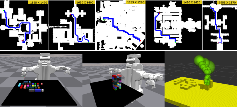
Figure 1: (Top: 2D Grid World) 5 scaled MovingAI maps with the start state shown in green, the goal state shown in red and the computed path shown in blue. (Bottom: Manipulation) The PR2 has to arrange a set of blocks on the table (left) into a given configuration (middle) with a motion planner (right) to compute Place actions.

Manipulation

We also evaluate GePA*SE in a manipulation planning domain for a task of assembling a set of blocks on a table into a given structure by a PR2 (Fig. 1 bottom). We collect a problem set of Place actions for 40 assembly tasks in each of which the blocks are arranged in random order on the table. Place requires a motion planner internally to compute collision-free trajectories for the 7-DoF right arm of the PR2 in a cluttered workspace to place the blocks at their desired pose. $\mathcal{A}^{c}$ comprises 22 static motion primitives that move one joint at a time by 4 or 7 degrees in either direction. $\mathcal{A}^{e}$ comprises a single dynamically generated primitive that attempts to connect the expanded state to a goal configuration ($r^{c}=20$). This primitive involves solving an optimization-based IK problem to find a valid configuration space goal and then collision checking of a linearly interpolated path from the expanded state to the goal state. All primitives have a uniform cost. A backward BFS in the workspace ($x,y,z$) is used to compute the heuristic with an inflation factor of $w=\epsilon=100$. For the problem set generation, we use w-GePA*SE with 6 threads and a large timeout. We then evaluate all the algorithms with different thread budgets on this problem set with a timeout of $2$ $\mathrm{s}$. In the computation of the metrics (Table 1 bottom), we only consider the set of problems that are successfully solved and lead to a path length longer than 2 states for all algorithms. This is needed to not skew the statistics by the cases where the IK-based primitive connects the start state directly to the goal without any meaningful planning effort. We see that w-GePA*SE consistently achieves the lowest mean planning times while maintaining a high success rate across all thread budgets. In this domain, the best baseline based on mean planning time (underlined) varies with the thread budget.

Conclusion

We presented GePA*SE, a generalized formulation of two parallel search algorithms i.e. PA*SE and ePA*SE for domains with action spaces comprising a mix of cheap and expensive to evaluate actions. We showed that by employing different parallelization strategies for edges based on the computation effort required to evaluate them, GePA*SE achieves higher efficiency. We demonstrated this on several planning domains.

References

- Cohen, Chitta, and Likhachev (2014) Cohen, B.; Chitta, S.; and Likhachev, M. 2014. Single-and dual-arm motion planning with heuristic search. The International Journal of Robotics Research, 33(2): 305–320.
- Devaurs, Siméon, and Cortés (2011) Devaurs, D.; Siméon, T.; and Cortés, J. 2011. Parallelizing RRT on distributed-memory architectures. In 2011 IEEE International Conference on Robotics and Automation, 2261–2266.
- Evett et al. (1995) Evett, M.; Hendler, J.; Mahanti, A.; and Nau, D. 1995. PRA*: Massively parallel heuristic search. Journal of Parallel and Distributed Computing, 25(2): 133–143.
- He et al. (2021) He, X.; Yao, Y.; Chen, Z.; Sun, J.; and Chen, H. 2021. Efficient parallel A* search on multi-GPU system. Future Generation Computer Systems, 123: 35–47.
- Ichnowski and Alterovitz (2012) Ichnowski, J.; and Alterovitz, R. 2012. Parallel sampling-based motion planning with superlinear speedup. In IROS, 1206–1212.
- Irani and Shih (1986) Irani, K.; and Shih, Y.-f. 1986. Parallel A* and AO* algorithms- An optimality criterion and performance evaluation. In 1986 International Conference on Parallel Processing, University Park, PA, 274–277.
- Jacobs et al. (2012) Jacobs, S. A.; Manavi, K.; Burgos, J.; Denny, J.; Thomas, S.; and Amato, N. M. 2012. A scalable method for parallelizing sampling-based motion planning algorithms. In 2012 IEEE International Conference on Robotics and Automation, 2529–2536.
- Jacobs et al. (2013) Jacobs, S. A.; Stradford, N.; Rodriguez, C.; Thomas, S.; and Amato, N. M. 2013. A scalable distributed RRT for motion planning. In 2013 IEEE International Conference on Robotics and Automation, 5088–5095.
- Kusnur et al. (2021) Kusnur, T.; Mukherjee, S.; Saxena, D. M.; Fukami, T.; Koyama, T.; Salzman, O.; and Likhachev, M. 2021. A planning framework for persistent, multi-uav coverage with global deconfliction. In Field and Service Robotics, 459–474. Springer.
- Liang et al. (2021) Liang, J.; Sharma, M.; LaGrassa, A.; Vats, S.; Saxena, S.; and Kroemer, O. 2021. Search-Based Task Planning with Learned Skill Effect Models for Lifelong Robotic Manipulation. arXiv preprint arXiv:2109.08771.
- Mukherjee, Aine, and Likhachev (2022a) Mukherjee, S.; Aine, S.; and Likhachev, M. 2022a. ePA*SE: Edge-Based Parallel A* for Slow Evaluations. In International Symposium on Combinatorial Search, volume 15, 136–144. AAAI Press.
- Mukherjee, Aine, and Likhachev (2022b) Mukherjee, S.; Aine, S.; and Likhachev, M. 2022b. MPLP: Massively Parallelized Lazy Planning. IEEE Robotics and Automation Letters, 7(3): 6067–6074.
- Mukherjee et al. (2021) Mukherjee, S.; Paxton, C.; Mousavian, A.; Fishman, A.; Likhachev, M.; and Fox, D. 2021. Reactive long horizon task execution via visual skill and precondition models. In 2021 IEEE/RSJ International Conference on Intelligent Robots and Systems (IROS), 5717–5724. IEEE.
- Phillips, Likhachev, and Koenig (2014) Phillips, M.; Likhachev, M.; and Koenig, S. 2014. PA* SE: Parallel A* for slow expansions. In Twenty-Fourth International Conference on Automated Planning and Scheduling.
- Russell (2010) Russell, S. J. 2010. Artificial intelligence a modern approach. Pearson Education, Inc.
- Sturtevant (2012) Sturtevant, N. 2012. Benchmarks for Grid-Based Pathfinding. Transactions on Computational Intelligence and AI in Games, 4(2): 144 – 148.
- Zhou and Zeng (2015) Zhou, Y.; and Zeng, J. 2015. Massively parallel A* search on a GPU. In Proceedings of the AAAI Conference on Artificial Intelligence.