Prevalence of multistationarity and
absolute concentration robustness in reaction networks

Abstract.

For reaction networks arising in systems biology, the capacity for two or more steady states, that is, multistationarity, is an important property that underlies biochemical switches. Another property receiving much attention recently is absolute concentration robustness (ACR), which means that some species concentration is the same at all positive steady states. In this work, we investigate the prevalence of each property while paying close attention to when the properties occur together. Specifically, we consider a stochastic block framework for generating random networks, and prove edge-probability thresholds at which – with high probability – multistationarity appears and ACR becomes rare. We also show that the small window in which both properties occur only appears in networks with many species. Taken together, our results confirm that, in random reversible networks, ACR and multistationarity together, or even ACR on its own, is highly atypical. Our proofs rely on two prior results, one pertaining to the prevalence of networks with deficiency zero, and the other “lifting” multistationarity from small networks to larger ones.

Keywords: Multistationarity, absolute concentration robustness, random graph, stochastic block model, threshold function, reaction network.

1. Introduction

In biochemical reaction networks, multistationarity is often a desirable phenomenon, as it is associated with biochemical switches, cellular signaling, and decision-making [32]. A network is multistationary when there are two or more compatible positive steady states; “compatible” means that the steady states have the same conserved quantities such as total mass. Which reaction networks are multistationary? This question has a long history, and many results have been established (see the survey [25]).

Another significant property exhibited by some biochemical reaction networks is absolute concentration robustness (ACR), which refers to when a steady-state species concentration is maintained even when initial conditions are changed. The concept of ACR was first popularized by Shinar and Feinberg in 2010 [29] and has since attracted much interest both from the mathematical standpoint [2, 23, 28, 22] and in applications [13, 27].

While each of these two properties has been studied in isolation, their relationship is not well understood. Nonetheless, multistationarity and ACR can be viewed as opposite behaviors, as multiple steady states cannot be in general position if ACR is present. Indeed, known examples of networks having ACR (for instance, those in [29]) typically are non-multistationary.

Accordingly, the driving motivation of this article is to explore the relationship between multistationarity and ACR and to investigate the prevalence of networks with either property. However, it is generally challenging to assess multistationarity and ACR [25, 28]. Therefore, following the approach of Anderson and Nguyen [6, 7], we instead investigate the prevalence of these properties in randomly generated reaction networks. Specifically, we prove asymptotic results on the probability that such a network has either property, as the number of species goes to infinity.

A summary of our results appears in Table 1, which pertains to when reaction networks are randomly generated by a certain stochastic block model in which the expected numbers of reactions of each “type” are roughly of the same magnitude. Here, the type refers to which forms of complexes – $0,X_{i},2X_{i},X_{i}+X_{j}$ – appear in the reaction (notice that we restrict our attention to at-most-bimolecular networks, which encompass most reaction networks arising in biochemistry). We prove edge-probability thresholds for the resulting reaction networks to be nondegenerately multistationary or to preclude ACR (Theorem 4.8), and a restatement of this result in terms of the expected number of edges (that is, reactions) is in Table 1.

Expected number of reactions	Multistationary?	ACR?
Asymptotically greater than $1$, but less than $n^{2/3}$	No	Yes
Asymptotically greater than $n$, but less than $\frac{2}{17}n(\log(n)-c(n))$,	Yes	Yes
for some $c(n)\to\infty$
Greater than $n(\log(n)+c(n))$, for some $c(n)\to\infty$	Yes	No

Table 1. For random reaction networks, with $n$ species, generated by a certain stochastic block model, this table lists ranges for the expected number of reactions, and whether – with high probability – such a network is multistationary or has ACR. For further details, see Theorem 4.8 and Remark 4.11.

We see from Table 1 that the window for having both multistationarity and ACR is relatively small: when the expected number of edges is asymptotically between $n$ and $\frac{2}{17}n\log(n)$. In fact, in this window, which only appears when there are thousands of species (Remark 4.14), the ACR species either appears by itself without interacting with other species (in essence, the network decouples) or it appears as a catalyst (Remark 4.22). We therefore expect that reaction networks with both multistationarity and ACR, in which the ACR species interacts nontrivially with other species, are rare and may require special structures or constructions.

Our proofs rely crucially on two prior results. The first, due to Anderson and Nguyen, pertains to the prevalence of certain networks that are known to preclude multistationarity, namely, networks with deficiency zero (specifically, the result asserts that “sparse” reaction networks are likely to have deficiency zero) [6, 7]. The second result concerns “lifting” multistationarity from small networks to larger ones [8, 10, 24], which we use to show the high probability of multistationarity and the absence of ACR in “dense” reaction networks.

This article is structured as follows: Section 2 introduces reaction networks, multistationarity, and ACR. Section 3 contains our results on the prevalence of multistationarity and ACR in random reaction networks via edge-probability thresholds. In Section 4, we introduce the type-homogeneous stochastic block model, which we use to generate random reaction networks, and compute explicitly the thresholds for multistationarity and ACR. We end with a discussion in Section 5.

2. Background

Here, we recall the basic setup and definitions involving reaction networks (Section 2.1), the dynamical systems they generate (Section 2.2), and absolute concentration robustness (Section 2.3). (A more detailed exposition can be found in [18].) We also discuss how multistationarity and ACR are affected when adding new reactions to an existing network (Section 2.4).

2.1. Reaction networks

A reaction network $G$ is a directed graph in which the vertices are non-negative linear combinations of species $X_{1},X_{2},\ldots,X_{n}$. As is standard in reaction network theory, we refer to each vertex as a complex, and we denote the $i$-th complex by $y_{i}=y_{i1}X_{1}+y_{i2}X_{2}+\dots+y_{in}X_{n}$ or by $y_{i}=(y_{i1},y_{i2},\dots,y_{in})$ (where $y_{ij}\in\mathbb{Z}_{\geq 0}$).

Edges of $G$ represent the possible changes in the abundances of the species, and are referred to as reactions. It is standard to represent a reaction $(y_{i},y^{\prime}_{i})$ by the notation $y_{i}\to y^{\prime}_{i}$. In such a reaction, $y_{i}$ is the reactant complex, and $y^{\prime}_{i}$ is the product complex. A species $X_{k}$ is a catalyst-only species of a reaction $(y_{i},y^{\prime}_{i})$ if the stoichiometric coefficient of $X_{k}$ is the same in the product and reactant (that is, $y_{ik}=y^{\prime}_{ik}$). Finally, a reaction network $G^{\prime}$ is a subnetwork of a network $G$ if the sets of species, complexes, and reactions of $G^{\prime}$ are subsets of the respective sets of $G$.

In examples, it is often convenient to write species as $A,B,C,\dots$ rather than $X_{1},X_{2},X_{3},\dots$. Additionally, we typically depict a reaction network by its set of reactions, in which case the sets of species and complexes are implied.

Example 2.1.

The reaction network $\{A+B\to 2B,~{}B\to A\}$ has 2 species (namely, $A$ and $B$), 4 complexes ($A+B,~{}2B,~{}B,~{}A$), and 2 reactions. ∎

A reaction network is reversible if every edge in the graph is bidirected.

Example 2.2.

The reaction network $\{A\leftrightarrows B+C,~{}0\leftrightarrows A,~{}0\leftrightarrows B,~{}C\leftrightarrows 2C\}$ is reversible. ∎

This article focuses on at-most-bimolecular reaction networks (or, for short, bimolecular), which means that every complex $y_{i}$ of the network satisfies $y_{i1}+y_{i2}+\dots+y_{in}\leq 2$ (where $n$ is the number of species). Equivalently, each complex has the form $0$, $X_{i}$, $X_{i}+X_{j}$, or $2X_{i}$ (where $X_{i}$ and $X_{j}$ are species). The reaction networks in Examples 2.1–2.2 are bimolecular.

2.2. Dynamical system arising from a network

Under the assumption of mass-action kinetics, each reaction network $G$ defines a parametrized family of systems of ordinary differential equations (ODEs), as follows. Let $r$ denote the number of reactions of $G$. We write the $i$-th reaction as $y_{i}\to y_{i}^{\prime}$ and assign a positive rate constant $\kappa_{i}\in\mathbb{R}_{>0}$ to the corresponding reaction.

The mass-action system, denoted by $(G,\kappa)$, where $\kappa=(\kappa_{1},\kappa_{2},\dots,\kappa_{r})$, is the dynamical system arising from the following ODEs:

(1) $$\frac{dx}{dt}~{}=~{}\sum_{i=1}^{r}\kappa_{i}x^{y_{i}}(y_{i}^{\prime}-y_{i})~{}=:~{}f_{\kappa}(x)~{},$$

where $x_{i}(t)$ denotes the concentration of the $i$-th species at time $t$ and $x^{y_{i}}:=\prod_{j=1}^{n}x_{j}^{y_{ij}}$. The right-hand side of the ODEs (1) consists of polynomials $f_{\kappa,i}$, for $i=1,2,\dots,n$ (where $n$ is the number of species). For simplicity, we often write $f_{i}$ instead of $f_{\kappa,i}$.

The stoichiometric subspace of $G$, which we denote by $S$, is the linear subspace of $\mathbb{R}^{n}$ spanned by all reaction vectors $y_{i}^{\prime}-y_{i}$ (for $i=1,2,\dots,r$). When $\text{dim}(S)=n$, we say that $G$ is full dimensional. Observe that the vector field of the mass-action ODEs (1) lies in $S$ (more precisely, the vector of ODE right-hand sides is always in $S$). Hence, a forward-time solution $\{x(t)\mid t\geq 0\}$ of (1), with initial condition $x(0)\in\mathbb{R}_{>0}^{n}$, remains in the following stoichiometric compatibility class [18]:

$$P_{x(0)}~{}:=~{}(x(0)+S)\cap\mathbb{R}_{\geq 0}^{n}~{}.$$

Example 02.1 (continued).

The network $\{A+B\overset{\kappa_{1}}{\rightarrow}2B,~{}B\overset{\kappa_{2}}{\rightarrow}A\}$ generates the following mass-action ODEs (1):

$$\frac{dx_{1}}{dt}~{}=~{}-\kappa_{1}x_{1}x_{2}+\kappa_{2}x_{2}$$

$$\frac{dx_{2}}{dt}~{}=~{}\kappa_{1}x_{1}x_{2}-\kappa_{2}x_{2}.$$

Moreover, it has a one-dimensional stoichiometric subspace (spanned by the vector $(1,0)^{\top}$). ∎

A steady state of a mass-action system is a nonnegative concentration vector $x^{*}\in\mathbb{R}_{\geq 0}^{n}$ at which the right-hand side of the ODEs (1) vanishes: $f_{\kappa}(x^{*})=0$. Our primary interest in this work is in positive steady states $x^{*}\in\mathbb{R}_{>0}^{n}$. Also, a steady state $x^{*}$ is nondegenerate if $\text{Im}(df_{\kappa}(x^{*})|_{S})=S$, where $df_{\kappa}(x^{*})$ is the Jacobian matrix of $f_{\kappa}$ evaluated at $x^{*}$, and $S$ is the stoichiometric subspace.

We consider multistationarity at two levels: systems and networks. A mass-action system $(G,\kappa)$ is multistationary (respectively, nondegenerately multistationary) if there exists some stoichiometric compatibility class having more than one positive steady state (respectively, nondegenerate positive steady state). A reaction network $G$ is multistationary if there exist positive rate constants $\kappa$ such that $(G,\kappa)$ is multistationary. Similarly, a network $G$ can be nondegenerately multistationary.

Example 2.3 (Multistationary system).

Consider the mass-action system generated by:

(2) $$\left\{A\stackrel{{\scriptstyle[}}{{1}}]{1}{\leftrightarrows}B+C,\quad 0\stackrel{{\scriptstyle[}}{{6}}]{1}{\leftrightarrows}A,\quad 0\stackrel{{\scriptstyle[}}{{2}}7]{1}{\leftrightarrows}B,\quad C\stackrel{{\scriptstyle[}}{{8}}]{1}{\leftrightarrows}2C\right\}~{}.$$

It is straightforward to check (or compute) that there are exactly three positive steady states, namely, $(13,20,1),(18,15,2),(21,12,3)$, and all three are nondegenerate. ∎

2.3. Deficiency and absolute concentration robustness

The deficiency of a reaction network $G$ is $\delta=v-\ell-\text{dim}(S)$, where $v$ is the number of vertices (or complexes) of $G$, $\ell$ is the number of connected components of $G$, and $S$ is the stoichiometric subspace. This invariant is central to many classical results pertaining to mass-action systems (1) [3, 4, 5, 17, 20, 21], including a structural criterion for absolute concentration robustness (ACR) [29], the topic we turn to next.

ACR, like multistationarity, is analyzed at the level of systems and also networks.

Definition 2.4 (ACR).

Let $X_{i}$ be a species of a reaction network $G$ with $r$ reactions.

1. For a fixed vector of positive rate constants $\kappa\in\mathbb{R}^{r}_{>0}$, the mass-action system $(G,\kappa)$ has absolute concentration robustness (ACR) in $X_{i}$ if $(G,\kappa)$ has a positive steady state and in every positive steady state $x\in\mathbb{R}_{>0}^{n}$ of the system, the value of $x_{i}$ (the concentration of $X_{i}$) is the same. This value of $x_{i}$ is the ACR-value of $X_{i}$.

2. The reaction network $G$ has unconditional ACR in species $X_{i}$ if the mass-action system $(G,\kappa)$ has ACR in $X_{i}$ for all $\kappa\in\mathbb{R}^{r}_{>0}$.

When $G$ has unconditional ACR in $X_{i}$, the property of ACR in $X_{i}$ holds across all rate constants, but the ACR-value can (and typically does) change with rate constants, as in the next example.

Example 02.1 (continued).

We return to the following network: $\{A+B\xrightarrow{\kappa_{1}}2B,~{}B\xrightarrow{\kappa_{2}}A\}.$ This network is a classical example of a network with ACR [29]. Indeed, at all positive steady states, the concentration of species $A$ is $\kappa_{2}/\kappa_{1}$, and hence the network has unconditional ACR in $A$. ∎

Remark 2.5 (ACR and reversible networks).

In Definition 2.4, ACR requires the existence of a positive steady state. This requirement is not included in some definitions of ACR in the literature. However, in this work, we focus on the reversible networks, which guarantees the existence of positive steady states (this result is due to Deng et al. [14] and Boros [12]). Hence, our results are valid with or without the requirement of positive steady states.

In the literature, reaction networks with ACR are typically not multistationary. Nonetheless, a network can both have ACR (in some species) and be multistationary. A simple example can be constructed by joining two networks, with disjoint species sets, where one network has ACR and the other is multistationary. A less trivial example can be generated by having the ACR species participate as an enzyme – more precisely, as a catalyst-only species – in the multistationary network. We illustrate this in the following example.

Example 2.6 (A network with multistationarity and ACR).

Consider the following network, in which $A$ is a catalyst-only species in the first two reactions:

$$\left\{A\stackrel{{\scriptstyle[}}{{\kappa}}_{1}]{\kappa_{2}}{\leftrightarrows}A+B,\quad 2B\stackrel{{\scriptstyle[}}{{\kappa}}_{3}]{\kappa_{4}}{\leftrightarrows}3B,\quad A\stackrel{{\scriptstyle[}}{{\kappa}}_{5}]{\kappa_{6}}{\leftrightarrows}2A\right\}~{}.$$

This network, which we call $G$, generates the following mass-action ODEs (1):

$$\frac{dx_{1}}{dt}~{}=~{}\kappa_{5}x_{1}-\kappa_{6}x_{1}^{2}$$

$$\frac{dx_{2}}{dt}~{}=~{}\kappa_{1}x_{1}-\kappa_{2}x_{1}x_{2}+\kappa_{3}x_{2}^{2}-\kappa_{4}x_{2}^{3}.$$

One can check directly that $G$ has unconditional ACR in species $A$ with ACR-value $\kappa_{5}/\kappa_{6}$. Moreover, for reaction rates $(\kappa_{1},\kappa_{2},\ldots,\kappa_{6})=(\frac{1}{512},\frac{1}{16},1,1,2,1)$, we obtain exactly $3$ positive steady states, with the following approximate values: $(2,0.050987),$ $(2,0.0890928)$, and $(2,0.85992)$. ∎

It is not straightforward to find non-trivial examples of reaction networks with multistationarity and unconditional ACR where the network cannot be decomposed into individual pieces, each with only one of the two properties. While such networks do exist, this is a topic of study unto its own. We will report on several families of such networks and their operating principles in future work.

In this work, we are interested in asymptotic results (as the size of the network grows) on the prevalence of multistationarity and ACR. An important tool we use for proving thresholds for these properties (or the lack thereof) is the network in the following example.

Example 02.3 (continued).

Consider again the following mass-action system:

$$\left\{A\stackrel{{\scriptstyle[}}{{1}}]{1}{\leftrightarrows}B+C,\quad 0\stackrel{{\scriptstyle[}}{{6}}]{1}{\leftrightarrows}A,\quad 0\stackrel{{\scriptstyle[}}{{2}}7]{1}{\leftrightarrows}B,\quad C\stackrel{{\scriptstyle[}}{{8}}]{1}{\leftrightarrows}2C\right\}~{},$$

which we saw has three positive steady states: $(13,20,1),(18,15,2),(21,12,3)$. By inspection, this system has no ACR (in any species) and hence the network does not have unconditional ACR. ∎

We end this subsection by recalling what is known about multistationarity and ACR for networks with deficiency 0. In the following result, part (1) follows from the deficiency-zero theorem [20] and part (2) is immediate from a recent result of Joshi and Craciun [23, Theorem 6.1].

Lemma 2.7.

If $G$ is a reaction network that has deficiency 0, then:

1. $G$ is not multistationary, and

2. if $G$ contains an inflow or outflow reaction (that is, a reaction of the form $0\to X_{i}$ or $0\leftarrow X_{i}$, for some species $X_{i}$), then $G$ has unconditional ACR (in some species).

2.4. Monotonicity of multistationarity and non-ACR with respect to adding reactions

This subsection pertains to how multistationarity and ACR are affected as we add new reactions to a reaction network. The following proposition essentially follows from recent results on “lifting” multistationarity from smaller networks to larger ones [8, 10, 24].

Lemma 2.8 (Lifting multistationarity or non-ACR).

Let $G$ be a full-dimensional network, and let $G^{\prime}$ be a network obtained by adding to $G$ a reaction that involves no new species (new complexes are allowed).

• If $G$ is nondegenerately multistationary, then so is $G^{\prime}$.

• If there exists a vector of positive rate constants $\kappa^{*}$ such that $(G,\kappa^{*})$ is nondegenerately multistationary and also does not have ACR (in any species), then the network $G^{\prime}$ does not have unconditional ACR in any species.

Proof.

Part $(i)$ follows directly from [24, Theorem 3.1].

For part $(ii)$, suppose that there exists $\kappa^{*}$ such that $(G,\kappa^{*})$ does not have ACR (in any species) and also has nondegenerate, positive steady states $q_{1},q_{2},\dots,q_{m}$, where $m\geq 2$. We denote each steady state by $q_{i}=(q_{i,1},\ldots,q_{i,n})\in\mathbb{R}^{n}_{\geq 0}$ (for $i=1,\ldots,m$), where $n$ is the number of species of $G$.

Let $\epsilon$ denote the rate constant of the reaction added to $G$ to obtain $G^{\prime}$. From the proof of [24, Theorem 3.1], there exists $\epsilon_{0}>0$ such that if $0<\epsilon<\epsilon_{0}$, then $(G^{\prime},(\kappa;\epsilon))$ has nondegenerate, positive steady states $q_{1}(\epsilon),q_{2}(\epsilon),\ldots,q_{m}(\epsilon)$ such that $\lim_{\epsilon\to 0^{+}}q_{i}(\epsilon)=q_{i}$ (for all $i$).

Next, consider some species $X_{\ell}$ (so, $1\leq\ell\leq n$). As $(G,\kappa^{*})$ does not have ACR in $X_{\ell}$, there exist steady states $q_{i}$ and $q_{j}$ at which the corresponding concentrations of $X_{\ell}$ differ (that is, $q_{i,\ell}\neq q_{j,\ell}$). So, as $\lim_{\epsilon\to 0^{+}}q_{i}(\epsilon)=q_{i}$ and $\lim_{\epsilon\to 0^{+}}q_{j}(\epsilon)=q_{j}$, there exists $\epsilon_{\ell}>0$ (with $\epsilon_{\ell}<\epsilon_{0}$) such that if $0<\epsilon<\epsilon_{\ell}$, then $|q_{i,\ell}(\epsilon)-q_{j,\ell}(\epsilon)|>0$ and hence $(G^{\prime},(\kappa^{*};\epsilon))$ does not have ACR in $X_{\ell}$.

Finally, we pick $\epsilon$ such that $0<\epsilon<\min_{\ell}\epsilon_{\ell}$. By construction, the system $(G^{\prime},(\kappa^{*};\epsilon))$ does not have ACR in any species. Hence, $G^{\prime}$ does not have unconditional ACR. ∎

Remark 2.9.

Lemma 2.8 implies that, given full dimensionality, nondegenerate multistationarity is a monotone increasing property (with respect to adding new edges/reactions).

3. Multistationarity and ACR in random reaction networks

In this section, we follow the approach in [6, 7] in which reaction networks are generated using a random-graph framework (Section 3.1). In Section 3.2, we prove the existence of thresholds for the presence or absence of nondegenerate multistationarity and unconditional ACR. These thresholds are with respect to increasing graph density, that is, the fraction of reactions present – among all possible reactions.

In this section, we use the following standard notation. For sequences of numbers $\{a_{n}\}$ and $\{b_{n}\}$, we write $a_{n}\ll b_{n}$ (or $b_{n}\gg a_{n}$) if

$$\lim_{n\to\infty}\frac{a_{n}}{b_{n}}=0~{};$$

and we write $a_{n}\sim b_{n}$ if

$$\lim_{n\to\infty}\frac{a_{n}}{b_{n}}=c~{},$$

for some positive constant $c$. Also, a sequence of events $\{A_{n}\}$ occurs with high probability (w.h.p.) if $\lim_{n\to\infty}\mathbb{P}(A_{n})=1$.

3.1. Random reaction networks

Consider the class of bimolecular reaction networks on $n$ species $X_{1},X_{2},\dots,X_{n}$. The set of all possible complexes is then

(3) $$V_{n}~{}=~{}\{0\}~{}\cup~{}\{X_{i}\mid 1\leq i\leq n\}~{}\cup~{}\{2X_{i}\mid 1\leq i\leq n\}~{}\cup~{}\{X_{i}+X_{j}\mid 1\leq i,j\leq n~{},~{}i\neq j\}.$$

The cardinality of $V_{n}$ is therefore given by

$$|V_{n}|~{}=~{}1+n+n+{n\choose 2}~{}=~{}\frac{n^{2}+3n+2}{2}~{}.$$

Definition 3.1 (Edge probabilities).

Let $n$ be a positive integer.

1. Consider two distinct vertices $u,v\in V_{n}$. An edge probability function for the unordered pair $e=(u,v)$ is a non-decreasing function, $\phi_{e}(p_{n})$, in a single parameter $p_{n}\in[0,1]$.

2. A choice of edge probabilities is a collection of edge probability functions, $\phi_{e}(p_{n})$, one for each unordered pair $e=(u,v)$ of vertices in $V_{n}$.

Definition 3.2 (Random graph $G(V_{n},p_{n})$).

Fix a positive integer $n$, some $p_{n}\in[0,1]$, and a choice of edge probabilities $\{\phi_{e}(p_{n})\}$. We generate random (undirected) graphs, which we denote by $G(V_{n},p_{n})$, as follows:

• the vertex set is $V_{n}$, and

• the probability that there is an edge between two vertices $u,v\in V_{n}$ is given by the corresponding edge probability function (where $e=(u,v)$):

  $$\mathbb{P}(e\text{ is an edge of }G(V_{n},p_{n}))~{}=~{}\phi_{e}(p_{n}).$$

Definition 3.3 (Random network $G_{n}$).

Each random graph $G(V_{n},p_{n})$ (generated by some choice of edge probabilities) defines a random reaction network, which we denote by $G_{n}$, consisting of reversible reactions, as follows:

• The set of species of $G_{n}$ is $\{X_{1},X_{2},\dots,X_{n}\}$.

• The (reversible) reactions of $G_{n}$ correspond to the edges of $G(V_{n},p_{n})$.

Recall from Section 2.1 that $G_{n}$ is full-dimensional if its dimension is $n$.

Remark 3.4.

It is possible that some species of $G_{n}$ appears in no complexes, especially when $G(V_{n},p_{n})$ is sparse (e.g., the network shown later in Figure 1). Such $G_{n}$ are not full-dimensional.

3.2. Thresholds for multistationarity and ACR

In this subsection, we show that for the random reaction networks defined in the prior subsection, there exist thresholds for the presence or absence of nondegenerate multistationarity and unconditional ACR (Theorem 3.7). Subsequently, we discuss the challenges of computing such thresholds, and then describe a strategy for proving upper bounds on the thresholds (see Corollary 3.14).

The following definition is useful in the proof of Theorem 3.7 and also later in Proposition 3.13.

Definition 3.5 ($S^{*}_{n}$).

For $n\in\mathbb{Z}_{\geq 1}$, let $S^{*}_{n}$ denote the set of all full-dimensional bimolecular networks $G$ with exactly $n$ species for which there exists a vector of rate constants $\kappa$ such that $(G,\kappa)$ is nondegenerately multistationary and also does not have ACR in any species.

Remark 3.6 ($S^{*}_{n}$ is nonempty for $n\geq 2$).

The set $S^{*}_{1}$ is empty [26], but for all $n\geq 2$, $S_{n}^{*}$ is nonempty. This is shown for $n\geq 3$ in Proposition 3.13, and $S^{*}_{2}$ contains the following network:

$$\left\{A+B\stackrel{{\scriptstyle[}}{{1}}/4]{1/32}{\leftrightarrows}2A,\quad 2B\stackrel{{\scriptstyle[}}{{1}}/4]{1}{\leftrightarrows}A,\quad\emptyset\stackrel{{\scriptstyle[}}{{1}}]{1}{\leftrightarrows}B\right\}~{}.$$

Indeed, the indicated rate constants generate a system with $3$ nondegenerate positive steady states – with approximate values $(0.419694,1.11107)$, $(2.65005,2.3128)$, and $(216.681,27.5757)$ – and so this system is nondegenerately multistationarity and also does not have ACR.

Theorem 3.7 (Thresholds for full-dimensionality, multistationarity, and non-ACR).

Consider the setup for generating random reaction networks $G_{n}$, described in Section 3.1, for some choice of edge probabilities. Then there exist threshold functions (“thresholds”, for short) $0<r_{0}(n)\leq r_{1}(n)\leq r_{2}(n)$, such that for any $\{p_{n}\}_{n\geq 1}$:

• If $p_{n}\gg r_{0}(n)$, then $G_{n}$ is full-dimensional w.h.p.

• If $p_{n}\gg r_{1}(n)$, then $G_{n}$ is full-dimensional and nondegenerately multistationary w.h.p.

• If $p_{n}\gg r_{2}(n)$, then $G_{n}$ is full-dimensional, is nondegenerately multistationary, and does not have unconditional ACR (in any species) w.h.p.

Proof.

Being a full-dimensional network is a monotone increasing property with respect to adding reactions (with no new species). This fact, combined with a well-known result from the theory of threshold functions [11], proves part (0).

From Remark 2.9, the property (for full-dimensional networks) of being nondegenerately multistationary is monotonically increasing with respect to adding reactions (with no new species). Exploiting again the theory of threshold functions [11], we obtain part (1).

Finally, Lemma 2.8(ii) and the theory of threshold functions together imply that there exists a threshold function $r_{2}(n)$ for $G_{n}$ to contain a subnetwork $H\in S^{*}_{n}$. This implies part (2). ∎

Theorem 3.7 implies that when a random network is sufficiently dense, it is multistationary w.h.p. (after a threshold $r_{1}(n)$) and also lacks unconditional ACR (after a threshold $r_{2}(n)$). However, computing these thresholds is generally difficult, because it is challenging to determine whether a large reaction network is multistationary and whether it precludes ACR. In fact, while there are sufficient conditions for ACR, such as the Shinar-Feinberg criterion [29], there are no easy-to-check necessary conditions for ACR (for general networks) [28, Section 2].

Nevertheless, there is a fruitful strategy for establishing upper bounds on the thresholds $r_{1}(n)$ and $r_{2}(n)$, which we describe in detail in the remainder of this subsection. The underlying idea comes from the fact (stated earlier in Lemma 2.8) that multistationarity can sometimes be lifted from a small subnetwork to the whole network. Therefore, in lieu of determining when multistationarity of the entire network emerges (as edge probabilities increase), we instead investigate when a small multistationary subnetwork emerges. The choice of edge probabilities dictates which such subnetworks emerge first. For the edge probabilities we consider in the next section, we focus on a particular multistationary subnetwork, as follows.

Definition 3.8 (Sets $S_{M,n}$ of multistationary motifs).

For $n\in\mathbb{Z}_{>0}$, let $S_{M,n}$ denote the set of all networks of the following form:

(4) $$\{X_{i}\leftrightarrows X_{j}+X_{k},\quad 0\leftrightarrows X_{i},\quad 0\leftrightarrows X_{j},\quad X_{k}\leftrightarrows 2X_{k}\}~{},$$

where $i,j,k$ are distinct indices with $1\leq i,j,k\leq n$. Each network (4) is a multistationary motif.

Remark 3.9.

Recall from Example 2.3 and Example  2.3 (continued) that each multistationary motif (4) is full-dimensional (3-dimensional) and nondegenerately multistationary, and does not have unconditional ACR (in any species).

Our next aim is to show (in Proposition 3.13 below) how to join a multistationary motif to another network (which we call a “lifting component”) so that the resulting network again is full-dimensional and nondegenerately multistationary, and lacks unconditional ACR.

Definition 3.10 (Sets $S_{L,k}$ of lifting components).

For $k\in\mathbb{Z}_{>0}$, let $S_{L,k}$ be the set of all reversible reaction networks for which the associated graph is a tree on $k$ vertices (that is, complexes), where each of the vertices has the form $X_{i}$ (for $i\in\mathbb{Z}_{>0}$). Every network in $S_{L,k}$ is a lifting component.

Example 3.11.

An example of a network (lifting component) in $S_{L,3}$ is $\{X_{2}\leftrightarrows X_{3}\leftrightarrows X_{4}\}$. ∎

Next, we describe a set of networks obtained by joining a multistationary motif (4), which has dimension $3$, to a lifting component of dimension $n-3$, so that the result is full-dimensional.

Definition 3.12 (Sets $S_{J,n}$ of joined multistationary motifs and lifting components).

For $n\geq 3$, let $S_{J,n}$ be the set of all reaction networks whose reactions can be written as the union of a network $G_{M}\in S_{M,n}$ and a network $G_{L}\in S_{L,n-2}$, such that $G_{M}$ and $G_{L}$ have exactly one species in common.

An example of such a joined network is shown later (see Figure 3 and Example 4.13).

Proposition 3.13 (Properties of $S_{J,n}$).

For $n\geq 3$, the following hold:

1. $S_{J,n}\subseteq S^{*}_{n}$. Consequently, every network $H\in S_{J,n}$ is full-dimensional and nondegenerately multistationary, and does not have unconditional ACR (in any species).

2. If some $H\in S_{J,n}$ is a subnetwork of a network $G$ with $n$ species, then $G$ is full-dimensional and nondegenerately multistationary, and does not have unconditional ACR (in any species).

Proof.

We first prove part (1). Let $H\in S_{J,n}$. By definition, there exist $G_{M}\in S_{M,n}$ and $G_{L}\in S_{L,n-2}$, with exactly one species in common, such that the reactions of $H$ are a union of those in $G_{M}$ and $G_{L}$. Relabel the species of $H$, if needed, so that $G_{M}$ is the following network:

$$\{X_{1}\leftrightarrows X_{2}+X_{3},\quad 0\leftrightarrows X_{1},\quad 0\leftrightarrows X_{2},\quad X_{3}\leftrightarrows 2X_{3}\}~{},$$

and also that the species of $G_{L}$ are $X_{\ell},X_{4},X_{5},\dots,X_{n}$, for some $\ell\in\{1,2,3\}$.

It is straightforward to check that $H$ is full-dimensional (that is, has dimension $n$). Thus, to show that $H\in S_{n}^{*}$, it suffices to show that there exists a vector of rate constants $\kappa$ such that $(H,\kappa)$ is nondegenerately multistationary and does not have ACR in any species. Accordingly, we define $\kappa$ as follows. First, we choose the rate constants for reactions in $G_{M}$ as in (2) in Example 2.3, so that $G_{M}$ has three nondegenerate, positive steady states: $(13,20,1),(18,15,2),(21,12,3)$. Next, fix all rate constants for reactions in $G_{L}$ to be $1$. Using the fact that $G_{L}$ is a spanning tree, a simple computation shows that the positive steady states are $(x_{\ell},x_{4},x_{5},\dots,x_{n})=(c,c,c,\dots,c)$, where $c$ is any positive real number, and these steady states are all nondegenerate.

We consider first the case when the common species is $X_{\ell}=X_{3}$. We claim that, in this case, the following are nondegenerate steady states of $(H,\kappa)$:

(5) $$(13,20,1,1,\dots,1),\quad(18,15,2,2,\dots,2),\quad(21,12,3,3,\dots,3)~{}.$$

To see this, let $\dot{x_{i}}=f_{i}$ for $i=1,2,3$, and $\dot{x_{i}}=g_{i}$ for $i=3,4,\dots,n$, denote the ODEs for $G_{M}$ and $G_{L}$, respectively, with rate constants as defined above. Hence, $(13,20,1),(18,15,2),(21,12,3)$ satisfy $f_{1}=f_{2}=f_{3}=0$, and $(1,1\dots,1),(2,2,\dots,2),(3,3,\dots,3)$ satisfy $g_{3}=g_{4}=\dots=g_{n}=0$. Next, the ODEs of $(H,\kappa)$ are as follows:

$$\dot{x_{i}}~{} =~{}f_{i}\quad\quad\quad{\rm for}~{}i=1,2$$

$$\dot{x_{3}}~{} =~{}f_{3}+g_{3}$$

$$\dot{x_{j}}~{} =~{}g_{j}\quad\quad\quad{\rm for}~{}j=4,\dots,n.$$

Hence, the vectors in (5) indeed are steady states of $(H,\kappa)$.

To show that the steady states (5) are nondegenerate, we must show that the Jacobian matrix of $(H,\kappa)$, when evaluated at each of these steady states, is nonsingular (recall that $H$ is full-dimensional). Since $G_{L}$ has mass conservation among the species $X_{3},X_{4},\dots,X_{n}$, we have $g_{3}+g_{4}+\dots+g_{n}=0$. Adding rows $4,5,\dots,n$ to row $3$ of the Jacobian matrix yields a triangular block matrix $\begin{bmatrix}A&0\\ B&C\end{bmatrix}$, where $A$ is the Jacobian matrix of $G_{M}$ and $C$ is obtained from the Jacobian matrix of $G_{L}$ by setting $x_{3}$ to 0. As both $A$ and $C$ are nonsingular, when evaluated at any of the positive steady states of its corresponding system, we conclude that the Jacobian matrix of $(H,\kappa)$, when evaluated at any of the steady states (5), is nonsingular, as desired.

By inspection of the steady states (5), we see that there is no ACR in any species. As for the remaining cases, when $X_{\ell}$ (the common species of $G_{M}$ and $G_{L}$) is $X_{1}$ or $X_{2}$, the argument is very similar to what is shown above and so the result holds in those cases, too.

Finally, part (2) follows directly from part (1) and Lemma 2.8. ∎

Corollary 3.14 (Bound on threshold $r_{2}$).

Consider the setup for generating random reaction networks $G_{n}$, described in Section 3.1, for some choice of edge probabilities. Let $r_{2}(n)$ be a threshold as defined in Theorem 3.7, and let $r_{2}^{\prime}(n)$ be the threshold for $G_{n}$ to contain, as a subnetwork, some $H\in S_{J,n}$. If $p_{n}\gg r_{2}^{\prime}(n)$, then $G_{n}$ is full-dimensional, is nondegenerately multistationary, and does not have unconditional ACR (in any species) w.h.p. Consequently, $\limsup\frac{r_{2}(n)}{r_{2}^{\prime}(n)}<\infty$.

Proof.

This result follows directly from Proposition 3.13 and Theorem 3.7. ∎

Remark 3.15.

In the next section, we show that for a certain choice of edge probabilities, the thresholds for full-dimensionality, multistationarity, and containing (as a subnetwork) a multistationary motif in $S_{M,n}$ coincide. That is, in this scenario, $r_{0}(n)=r_{1}(n)=r_{1}^{\prime}(n)$, where $r_{1}^{\prime}$ denotes the threshold for $G_{n}$ to contain a multistationary motif. (In fact, in this setting, once we pass the threshold for full-dimensionality, a multistationary motif emerges and furthermore its multistationarity can be lifted; see Theorem 4.8.) Intuitively, the reason a motif in $S_{M,n}$ is among the first small multistationary subnetworks to emerge is that it is fairly “generic”: it contains only a pair of reversible reactions and some flow reactions involving those species. Meanwhile, other small multistationary networks, such as the following (from [24]):

$$\{A\leftrightarrows A+B\leftrightarrows 2A,\quad\quad 0\leftrightarrows A,\quad\quad 0\leftrightarrows B\}~{},$$

may contain specific pathways such as $A\leftrightarrows A+B\leftrightarrows 2A$, where a species (here, $A$) must appear in all three complexes, and therefore such networks are expected to emerge at higher thresholds.

4. Multistationarity and ACR in type-homogeneous stochastic block model

The prior section considered general random graph models without specifying the edge probabilities. In this subsection, we introduce a specific choice of edge probabilities (Section 4.1) and then compute the resulting thresholds from Theorem 3.7 (see Theorem 4.8 in Section 4.2).

4.1. A stochastic block model

One possible choice of edge probabilities comes from the Erdős-Rényi random graph model; here, the edge probabilities are uniform (that is, every edge is equally likely). In this framework, reactions of the form $X_{i}+X_{j}\leftrightarrows X_{h}+X_{k}$ are overwhelmingly the most prominent [7]. However, this situation is unlikely to occur in biochemistry. Indeed, in applications, one expects to see various types of complexes and reactions, such as inflow and outflow reactions $0\leftrightarrows X_{i}$ or association and disassociation reactions $X_{i}+X_{j}\leftrightarrows X_{k}$.

Therefore, we instead consider a model in which reaction types are equally represented. This model is a specific case of the stochastic block models [19] introduced in [6]. To define this model, we need the following partitions of sets of vertices and edges:

Definition 4.1 ($C_{i}$ and $E_{i,j}$).

Let $n\geq 1$. Consider the following partition of the set of vertices $V_{n}$, as in (3), into 3 subsets:

1. $C_{0}=\{0\}$,

2. $C_{1}=\{aX_{i}\mid 1\leq i\leq n\ \text{ and }a\in\{1,2\}\}$,

3. $C_{2}=\{X_{i}+X_{j}\mid 1\leq i,j\leq n{\rm~{}and~{}}i\neq j\}$.

Let $E_{i,j}$ denote the set of (undirected) edges $(u,v)$ with $u\in C_{i}$ and $v\in C_{j}$; in particular:

1. $E_{0,1}=\{0\leftrightarrows aX_{i}\mid 1\leq i\leq n\text{ and }a\in\{1,2\}\}$,

2. $E_{0,2}=\{0\leftrightarrows X_{i}+X_{j}\mid 1\leq i,j\leq n\text{ and }i\neq j\}$,

3. $E_{1,1}=\{aX_{i}\leftrightarrows bX_{j}\mid 1\leq i,j\leq n,~{}a,b\in\{1,2\},\text{ and }(a,i)\neq(b,j)\}$,

4. $E_{1,2}=\{aX_{i}\leftrightarrows X_{j}+X_{k}\mid 1\leq i,j,k\leq n,~{}a\in\{1,2\},\text{ and }j\neq k\}$,

5. $E_{2,2}=\{X_{i}+X_{j}\leftrightarrows X_{k}+X_{h}\mid 1\leq i,j,k,h\leq n\text{ and }i\neq j,k\neq h,\text{ and }(i,j)\neq(k,h)\neq(j,i)\}$.

Two reactions in the same set $E_{i,j}$ have the same type.

Remark 4.2.

The sets $E_{0,1},E_{0,2},E_{1,1},E_{1,2},E_{2,2}$ partition the set of all possible edges of a graph with vertex set $V_{n}$. Also, $|C_{0}|=1$, $|C_{1}|\sim n$, and $|C_{2}|\sim n^{2}$. So, $|E_{i,j}|\sim n^{i+j}$ for $0\leq i\leq j\leq 2$.

In what follows, we denote the minimum of two numbers $a$ and $b$ as follows:

$$a\wedge b~{}:=\mathrm{min}(a,b)~{}.$$

Definition 4.3.

The type-homogeneous stochastic block model generates random graphs $G(V_{n},p_{n})$ with vertex set $V_{n}$ (as described in Definition 3.2) via the following choice of edge probabilities:

(6) $$\textrm{if }e\in E_{i,j},\textrm{ then }\mathbb{P}(e\text{ is an edge of }G(V_{n},p_{n}))~{}=~{}n^{4-i-j}p_{n}\wedge 1~{},$$

for all $0\leq i\leq j\leq 2$.

Remark 4.4.

In Definition 4.3, for vertices $u\in C_{i}$ and $v\in C_{j}$, the edge probability function (as in Definition 3.1) for the edge $e=(u,v)$ is given by $\phi_{e}(p_{n})=n^{4-i-j}p_{n}\wedge 1$. This edge probability function is readily seen to be non-decreasing in $p_{n}$.

Recall from Definition 3.3 that each random graph $G(V_{n},p_{n})$ generates a random reaction network $G_{n}$. The edge probabilities (6) ensure that, in $G_{n}$, the expected numbers of edges of each type are of the same magnitude (namely, $\sim n^{4}p_{n}$), whenever possible.

Example 4.5.

When $p_{n}=\frac{1}{n^{3.5}}$, the expected number of reactions of each type in $G_{n}$ is $\sim\sqrt{n}$. ∎

Example 4.6.

When $p_{n}=\frac{1}{n^{2.9}}$, $G_{n}$ contains all reactions in $E_{0,1}$ (since $n^{4-0-1}p_{n}\wedge 1=1$), and the expected number of reactions for each of the remaining types is $\sim n^{1.1}$. ∎

Remark 4.7.

When $p_{n}\gg\frac{1}{n^{3}}$ (for instance, $p_{n}=\frac{1}{n^{2.9}}$ in Example 4.6), $G_{n}$ contains all reactions in $E_{0,1}$, including all inflows/outflows $0\leftrightarrows X_{i}$, and so $G_{n}$ is full-dimensional.

In the next subsection, we see that the choice of $p_{n}$ in Example 4.5 generates networks $G_{n}$ that are not multistationary w.h.p., while the choice of $p_{n}$ in Example 4.6 generates networks that are multistationary and lack ACR w.h.p. (see Theorem 4.8).

4.2. Thresholds for multistationarity and ACR

For the type-homogeneous stochastic block model, the thresholds for nondegenerate multistationarity and (no) ACR are stated in the following theorem (which is proven later in Section 4.3).

Theorem 4.8 (Type-homogeneous stochastic block model).

Consider the setup for generating random reaction networks $G_{n}$, described in Section 3.1, for the edge probabilities given by (6). Then, for any $\{p_{n}\}_{n\geq 1}$:

1. (Sparse regime) If $\displaystyle\frac{1}{n^{4}}\ll p_{n}\ll\frac{1}{n^{10/3}}$, then w.h.p. $G_{n}$ has deficiency zero, is not multistationary, and has unconditional ACR (in some species).

2. (Dense regime, window of co-existence) If $\displaystyle\frac{1}{n^{3}}\ll p_{n}\leq\frac{\frac{2}{17}\log(n)-c(n)}{n^{3}}$ for some $c(n)\to\infty$, then w.h.p $G_{n}$ is nondegenerately multistationary and has unconditional ACR in some species.

3. (Dense regime) If $\displaystyle p_{n}\geq\frac{\log(n-2)+c(n)}{n^{2}(n-2)}$ for some $c(n)\to\infty$, then w.h.p. $G_{n}$ is nondegenerately multistationary and does not have unconditional ACR (in any species).

Remark 4.9.

When $p_{n}\ll\frac{1}{n^{4}}$, the expected number of reactions in $G_{n}$ is $\ll 1$. Accordingly, we do not consider this interval in Theorem 4.8.

Remark 4.10.

Theorem 4.8 immediately yields the following thresholds $r_{0}(n),r_{1}(n),r_{2}(n)$ (as defined in Theorem 3.7) for networks generated by the type-homogeneous stochastic block model:

$$r_{0}(n)~{}=~{}r_{1}(n)~{}=~{}\frac{1}{n^{3}}\quad{\rm and}\quad r_{2}(n)~{}=~{}\frac{\log(n)}{n^{3}}~{}.$$

Remark 4.11 (Thresholds via number of reactions).

Theorem 4.8 can be rephrased in terms of the expected number of edges (reactions) instead of edge-probability thresholds, as follows. For random reaction networks $G_{n}$ (with $n$ species) generated by the type-homogeneous stochastic block model, the following are implied directly by Theorem 4.8:

1. If the expected number of reactions of each type is $\gg 1$ and $\ll n^{2/3}$, then $G_{n}$ has deficiency zero and thus is not multistationary w.h.p.

2. If the expected number of reactions of each type is $\gg n$ but less than $\frac{2}{17}n(\log(n)-c(n))$ for some $c(n)\to\infty$, then $G_{n}$ is nondegenerately multistationariy and has unconditional ACR in some species w.h.p.

3. If the expected number of reactions of each type is greater than $n(\log(n)+c(n))$ for some $c(n)\to\infty$, then $G_{n}$ is nondegenerately multistationary and does not have unconditional ACR (in any species) w.h.p.

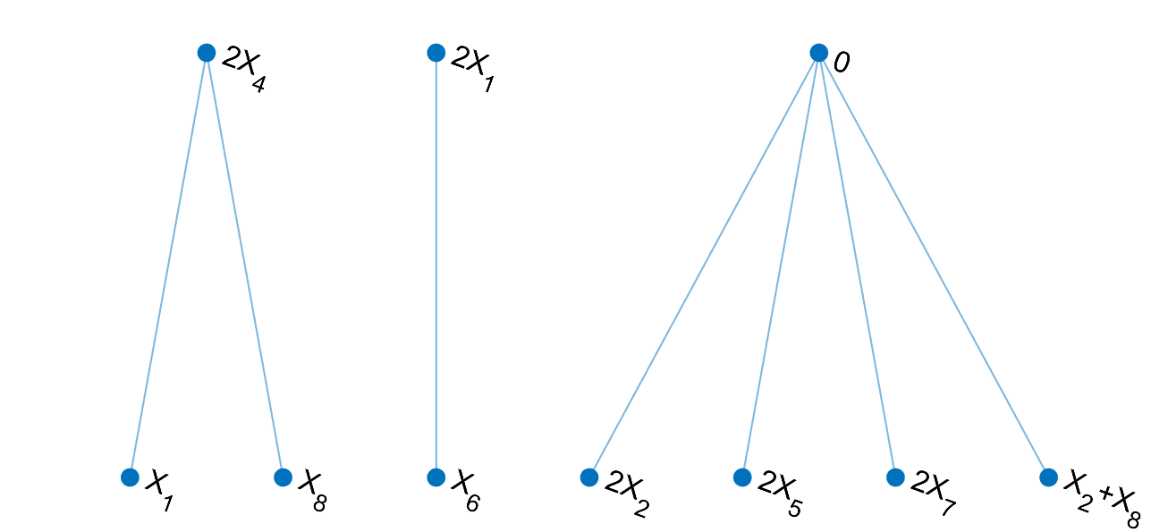
Figure 1. A realization of a random reaction network generated by the type-homogeneous stochastic block model in the sparse regime ($n=8$ species and $p_{n}=\frac{0.5}{n^{3.5}}$). Edges represent reversible reactions.

Example 4.12 (Sparse regime).

Figure 1 shows a realization of a random reaction network $G_{n}$ generated by the type-homogeneous stochastic block model with $n=8$ and $p_{n}=\frac{0.5}{n^{3.5}}$ (which is in the sparse regime). The following properties of $G_{n}$ are as expected from Theorem 4.8: The deficiency is $\delta=10-3-7=0$ and so $G_{n}$ is not multistationary, and it is easy to check that $G_{n}$ has unconditional ACR in all species except $X_{3}$ (which does not appear in any complex). ∎

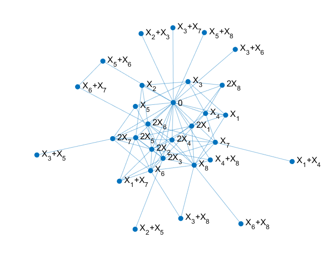
Figure 2. A realization of a random reaction network generated by the type-homogeneous stochastic block model in the dense regime ($n=8$ and $p_{n}=\frac{2.5}{n^{3}}$).

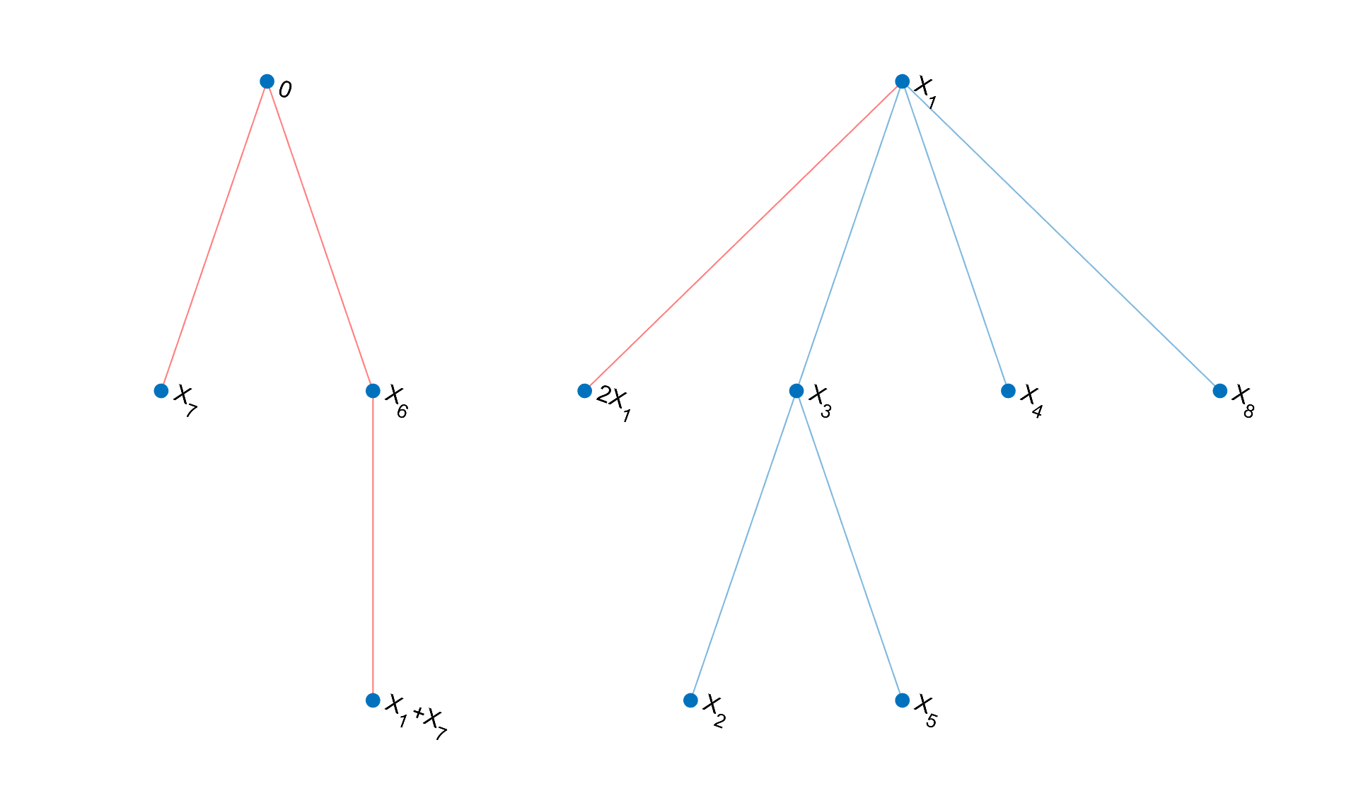
Figure 3. A subnetwork of the network in Figure 2, which is a union of a multistationary motif $M$ (red edges) and a lifting component $L$ (blue edges). Notice that $M$ and $L$ share exactly one species, namely, $X_{1}$.

Example 4.13 (Dense regime).

Figure 2 shows a realization of a random reaction network $G_{n}$ generated by the type-homogeneous stochastic block model with $n=8$ and $p_{n}=\frac{2.5}{n^{3}}$ (which is in the dense regime). Figure 3 depicts a subnetwork of $G_{n}$ that is a union of a multistationary motif and a lifting component with one species in common. We can now use Proposition 3.13 and Lemma 2.8 to assert that this subnetwork is multistationary and lacks ACR, and then “lift” these properties to $G_{n}$. Indeed, this approach underlies our proof of Theorem 4.8 in the dense regime. ∎

Remark 4.14 (Window of co-existence).

If the number of species satisfies $n<e^{17/2}\approx 4914.8$, then the small window between $\frac{1}{n^{3}}$ and $\frac{\frac{2}{17}\log(n)-c(n)}{n^{3}}$, in Theorem 4.8(ii), does not exist. Therefore, in the type-homogeneous stochastic block model, it is unlikely to observe a random network with both multistationarity and ACR, unless it has many species.

4.3. Proof of Theorem 4.8

Theorem 4.8 follows directly from Propositions 4.16 and 4.19–4.21 below. This subsection is devoted to proving these propositions, which requires the following lemma.

Lemma 4.15.

For all $n\geq 1$ and $0\leq x\leq 1$, the following inequality holds:

$$(1-x)^{n}~{}\leq~{}e^{-nx}~{}.$$

Proof.

If $x=1$, the inequality holds. For $0\leq x<1$, the result follows directly from the inequality $\log(1-x)\leq-x$ (which is easy to check) and the fact that the log function is increasing. ∎

4.3.1. Sparse regime

Our result for the sparse regime is Proposition 4.16 below. Its proof uses Lemma 2.7 and recent results on the prevalence of deficiency-zero networks [6] .

Proposition 4.16 (Sparse regime).

Consider random reaction networks $G_{n}$ generated by edge probabilities given by (6). If $\frac{1}{n^{4}}\ll p_{n}\ll\frac{1}{n^{10/3}}$, then, w.h.p. $G_{n}$ has deficiency zero, is not multistationary, and has unconditional ACR (in some species).

Proof.

Assume that $\frac{1}{n^{4}}\ll p_{n}\ll\frac{1}{n^{10/3}}$. It follows from [6, Theorem 5.1 and Example 10] that, w.h.p., the deficiency of $G_{n}$ is 0. Thus, w.h.p., the deficiency-zero theorem (Lemma 2.7(1)) applies and so $G_{n}$ is not multistationary. Additionally, by Lemma 2.7(2), to show that w.h.p. $G_{n}$ has unconditional ACR in some species, it suffices to show that w.h.p. $G_{n}$ contains an edge in $E_{0,1}$. The probability that any given edge in $E_{0,1}$ appears in $G_{n}$ is $n^{4-0-1}p_{n}=n^{3}p_{n}$, and there are $|E_{0,1}|=2n$ such edges, so:

(7) $$\mathbb{P}(G_{n}\text{ contains an edge in }E_{0,1})~{}=~{}1-\big{(}1-n^{3}p_{n})^{2n}~{}\geq~{}1-e^{-2n^{4}p_{n}}~{}.$$

(The inequality in (7) is due to Lemma 4.15.) Finally, using (7) and the assumption $p_{n}\gg\frac{1}{n^{4}}$, we obtain that $\lim_{n\to\infty}\mathbb{P}(G_{n}\text{ contains an edge in }E_{0,1})=1$. This concludes the proof. ∎

4.3.2. Dense regime

The proofs in this subsection make frequent use of the well-known second moment method (for example, see [1]). We summarize this approach in the following lemma.

Lemma 4.17.

Let $\{T_{n}\}$ be a sequence of non-negative random variables. If $\text{Var}(T_{n})\ll(\mathbb{E}T_{n})^{2}$, then $\lim\limits_{n\to\infty}\mathbb{P}(T_{n}>0)=1$.

Proof.

From the second moment method, we have

$$\mathbb{P}(T_{n}>0)~{}\geq~{}1-\frac{\text{Var}(T_{n})}{(\mathbb{E}T_{n})^{2}}.$$

Taking the limit (as $n\to\infty$) completes the proof. ∎

Next, we show that networks generated in the dense regime contain multistationary motifs (4) w.h.p. (see Figures 2 and 3 for an example).

Lemma 4.18.

Consider random reaction networks $G_{n}$ generated by edge probabilities given by (6). If $p_{n}\gg\frac{1}{n^{3}}$, then w.h.p. some multistationary motif in the set $S_{M,n}$ is a subnetwork of $G_{n}$.

Proof.

Assume $p_{n}\gg\frac{1}{n^{3}}$. Then $G_{n}$ contains all inflows/outflows $0\leftrightarrows X_{i}$ (recall Remark 4.7), so it suffices to show that w.h.p. $G_{n}$ contains a subnetwork of the following form, for some $i,j,k$ distinct:

(8) $$\{X_{k}\leftrightarrows 2X_{k},~{}X_{i}\leftrightarrows X_{j}+X_{k}\}~{}.$$

Consider the reactions in (8). First, $X_{k}\leftrightarrows 2X_{k}$ is in $E_{1,1}$, so its edge probability is $n^{2}p_{n}\wedge 1$. Next, for a fixed $k$, with $1\leq k\leq n$, there are $(n-1)(n-2)$ reactions of the form $X_{i}\leftrightarrows X_{j}+X_{k}$ with $i,j,k$ distinct. Each such reaction belongs to $E_{1,2}$ and so its edge probability is $np_{n}\wedge 1$.

We can reduce to considering only three cases: (1) when $p_{n}>\frac{1}{n}$ for all $n$, (2) when $\frac{1}{n^{2}}\leq p_{n}\leq\frac{1}{n}$ for all $n$, and (3) when $p_{n}<\frac{1}{n^{2}}$ for all $n$.

Case 1: $p_{n}>\frac{1}{n}$ for all $n$. In this case, $n^{2}p_{n}\wedge 1=1=np_{n}\wedge 1$. So, for all $n\geq 3$, $G_{n}$ contains a subnetwork of the form (8) (in fact, $G_{n}$ contains all possible such subnetworks).

Case 2: $\frac{1}{n^{2}}\leq p_{n}\leq\frac{1}{n}$ for all $n$. In this case, $n^{2}p_{n}\wedge 1=1$, so $G_{n}$ contains all reactions of the form $X_{k}\leftrightarrows 2X_{k}$. Hence, we need only show that w.h.p. $G_{n}$ contains at least one reaction of the form $X_{i}\leftrightarrows X_{j}+X_{k}$ with $i,j,k$ distinct. The probability of this event, which we call $E_{n}$, is as follows:

$$\mathbb{P}(E_{n})~{}=~{}1-(1-np_{n})^{n(n-1)(n-2)}~{}\geq~{}1-e^{-n^{2}(n-1)(n-2)p_{n}}~{}\to~{}1\quad\mathrm{(as}~{}n\to\infty\mathrm{)},$$

where the inequality is due to Lemma 4.15, and the limit comes from the fact that $p_{n}\geq\frac{1}{n^{2}}$.

Case 3: $p_{n}<\frac{1}{n^{2}}$ for all $n$. In this case, the edge probability for each reaction $X_{k}\leftrightarrows 2X_{k}$ (respectively, $X_{i}\leftrightarrows X_{j}+X_{k}$) is $n^{2}p_{n}$ (respectively, $np_{n}$).

For $1\leq k\leq n$, let $A_{k}$ denote the event that $G_{n}$ contains a subnetwork of the form (8), where $i\neq j$ and $i,j\neq k$. (The notation $A_{k,n}$ would be better for $A_{k}$, but we prefer to avoid excessive subscripts.) It follows that the probability of $A_{k}$ is:

(9) $$\mathbb{P}(A_{k})~{}=~{}n^{2}p_{n}\left(1-(1-np_{n})^{(n-1)(n-2)}\right)~{}.$$

Define the random variable $T_{n}:=\sum_{k=1}^{n}{1}_{A_{k}}$. We wish to show that $\lim_{n\to\infty}\mathbb{P}(T_{n}>0)=1$. By Lemma 4.17, it is enough to prove $\text{Var}(T_{n})\ll(\mathbb{E}T_{n})^{2}$. To this end, we first compute $\mathbb{E}T_{n}$, using (9):

(10) $$\mathbb{E}T_{n}~{}=~{}\sum_{k=1}^{n}\mathbb{P}(A_{k})~{}=~{}n^{3}p_{n}\left(1-(1-np_{n})^{(n-1)(n-2)}\right)~{}.$$

Next, Lemma 4.15 yields the first inequality here:

(11) $$(1-np_{n})^{(n-1)(n-2)}~{}\leq~{}e^{-n(n-1)(n-2)p_{n}}~{}\ll~{}1~{},$$

and the second inequality (limit) comes from the assumption that $p_{n}\gg\frac{1}{n^{3}}$. Hence, using (10), we obtain $\mathbb{E}T_{n}\sim n^{3}p_{n}$.

To compute $\text{Var}(T_{n})$, we consider the event $A_{h}\cap A_{k}$, where $h\neq k$. It is straightforward to check that $A_{h}\cap A_{k}$ occurs if and only if $G_{n}$ contains the reactions $X_{h}\leftrightarrows 2X_{h}$ and $X_{k}\leftrightarrows 2X_{k}$ and also one of the following:

1. a reaction of the form $X_{i}\leftrightarrows X_{h}+X_{k}$ (for some $i\neq h,k$), or

2. a reaction of the form $X_{i}\leftrightarrows X_{j}+X_{k}$ (for some $j\neq k,h$ and $i\neq j,k$) and a reaction of the form $X_{l}\leftrightarrows X_{m}+X_{h}$ (for some $m\neq h,k$ and $l\neq m,h$).

A direct computation now yields the following probability:

$$\mathbb{P}(A_{h}\cap A_{k}) ~{}=~{}(n^{2}p_{n})^{2}(1-(1-np_{n})^{n-2}+(1-np_{n})^{n-2}(1-(1-np_{n})^{(n-2)^{2}})^{2})$$

(12) $$~{}=~{}n^{4}p_{n}^{2}(1-2(1-np_{n})^{(n-1)(n-2)}+(1-np_{n})^{(n-2)(2n-3)})~{}.$$

Now we use equations (9), (10), and (4.3.2) to compute $\text{Var}(T_{n})$, as follows:

$$\text{Var}(T_{n}) ~{}=~{}\mathbb{E}(T_{n}^{2})-(\mathbb{E}T_{n})^{2}$$

$$~{}=~{}\sum_{k=1}^{n}\mathbb{P}(A_{k})+\sum_{h\neq k}\mathbb{P}(A_{h}\cap A_{k})-(\mathbb{E}T_{n})^{2}$$

$$~{}=~{}n^{3}p_{n}\left(1-(1-np_{n})^{(n-1)(n-2)}\right)+(n-1)n^{5}p_{n}^{2}\left(1-2(1-np_{n})^{(n-1)(n-2)}+(1-np_{n})^{(n-2)(2n-3)}\right)$$

(13) $$\quad\quad-n^{6}p_{n}^{2}\left(1-(1-np_{n})^{(n-1)(n-2)}\right)^{2}~{}.$$

We claim that $\text{Var}(T_{n})\ll n^{6}p_{n}^{2}$. Indeed, this follows in a straightforward way from (11) and (4.3.2), the limit $(1-np_{n})^{(n-2)(2n-3)}\ll 1$ (which is closely related to (11)), and the assumption $p_{n}\gg\frac{1}{n^{3}}$. Finally, having shown $\text{Var}(T_{n})\ll n^{6}p_{n}^{2}$ and $\mathbb{E}T_{n}\sim n^{3}p_{n}$, we get, as desired, $\text{Var}(T_{n})\ll(\mathbb{E}T_{n})^{2}$. ∎

Lemma 4.18 allows us to establish the threshold for nondegenerate multistationarity, as follows:

Proposition 4.19 (Multistationarity in dense regime).

Consider random reaction networks $G_{n}$ generated by edge probabilities in (6). If $p_{n}\gg\frac{1}{n^{3}}$, then $G_{n}$ is nondegenerately multistationary w.h.p.

Proof.

Assume $p_{n}\gg\frac{1}{n^{3}}$. By Lemma 4.18, w.h.p., $G_{n}$ contains (as a subnetwork) a multistationary motif $M\in S_{M,n}$ (which is $3$-dimensional and nondegenerately multistationary, as noted in Remark 3.9). Relabeling species, if needed, we may assume that the species of $M$ are $X_{1},X_{2},X_{3}$.

Next, $p_{n}\gg\frac{1}{n^{3}}$ implies that, w.h.p., $G_{n}$ contains all inflow/outflow reactions $0\leftrightarrows X_{i}$ (Remark 4.7), and in particular contains the $(n-3)$-dimensional subnetwork consisting of reactions $0\leftrightarrows X_{i}$, for all $i=4,5,\dots,n$, which we denote by $G^{\prime}$. As $M$ and $G^{\prime}$ have no species in common, the subnetwork of $G$ formed by the union of their reactions, which we denote by $N$, is full-dimensional ($n$-dimensional). It is straightforward to check that $N$ “inherits” nondegenerate multistationarity from $M$. (The proof is similar to that of Proposition 3.13(1).) Thus, by Lemma 2.8, $G_{n}$ is nondegenerately multistationary w.h.p. ∎

Proposition 4.20 (ACR in dense regime).

Consider random reaction networks $G_{n}$ generated by edge probabilities given by (6). If the following inequality holds:

(14) $$\displaystyle p_{n}~{}\geq~{}\frac{\log(n-2)+c(n)}{n^{2}(n-2)}~{},\quad\textrm{ for some }c(n)\to\infty~{},$$

then w.h.p. $G_{n}$ does not have unconditional ACR (in any species).

Proof.

Assume that inequality (14) holds. By Proposition 3.13(2), it suffices to show that, w.h.p., some $H\in S_{J,n}$ (as in Definition 3.12) is a subnetwork of $G_{n}$.

First, consider the case when $p_{n}\geq\frac{1}{n^{2}}$ for all $n$. Then, $p_{n}\gg\frac{1}{n^{3}}$, so by Lemma 4.18, $G_{n}$ contains, as a subnetwork, some multistationary motif $M\in S_{M,n}$. Next, we show that $G_{n}$ also contains all lifting components involving species $\{X_{1},X_{2},\dots,X_{n}\}$. Indeed, reactions of the form $X_{\ell}\leftrightarrows X_{m}$ are in $E_{1,1}$ and hence have edge-probability $n^{4-1-1}p_{n}\wedge 1=1$ (since $p_{n}\geq\frac{1}{n^{2}}$), and so $G_{n}$ contains all such reactions. Thus, as desired, w.h.p., $G_{n}$ contains some $H\in S_{J,n}$ as a subnetwork.

To complete the proof, we need only consider the following case:

(15) $$\displaystyle\frac{\log(n-2)+c(n)}{n^{2}(n-2)}~{}\leq~{}p_{n}~{}<~{}\frac{1}{n^{2}}~{},\quad\textrm{ for some }c(n)\to\infty~{}.$$

Recall from Remark 4.7 that, in this case, $G_{n}$ contains all reactions of the form $0\leftrightarrows X_{\ell}$. Thus, all vertices of the form $X_{\ell}$ appear in $G_{n}$. For positive integers $i\neq j$, let $G_{n}^{i,j}$ denote the subgraph of (the underlying graph of) $G_{n}$, induced by the following set of vertices of $G_{n}$: $\left\{X_{\ell}\mid\ell\in\{1,2,\dots,n\}\smallsetminus\{i,j\}\right\}$. Next, for distinct $i,j,k\in\{1,2,\dots,n\}$, let $A_{k,i,j}$ denotes the event that (i) $G_{n}^{i,j}$ is connected and (ii) $G_{n}$ contains the reactions $X_{k}\leftrightarrows 2X_{k}$ and $X_{i}\leftrightarrows X_{j}+X_{k}$.

We claim that, for $n$ sufficiently large, the event $A_{k,i,j}$ implies that $G_{n}$ contains some $H\in S_{J,n}$ as a subnetwork. To see this, first note that the inequality (15) implies that $p_{n}\gg\frac{1}{n^{3}}$ and so, for $n$ large enough, $G_{n}$ contains all flow reactions $0\leftrightarrows X_{\ell}$ (Remark 4.7). So, condition (ii) guarantees a multistationary motif $M$, for $n$ sufficiently large. Next, condition (i) and the fact that connected graphs have spanning trees yield a “complementary” lifting component $L$. By joining $M$ and $L$, we obtain some $H\in S_{J,n}$ as a subnetwork of $G_{n}$, as claimed.

Let $T_{n}=\sum_{k,i,j}1_{A_{k,i,j}}$ (where the sum is over distinct $i,j,k\in\{1,2,\dots,n\}$). To finish the proof, it suffices to show that $\lim_{n\to\infty}\mathbb{P}(T_{n}>0)=1.$ By Lemma 4.17, we need only show $\text{Var}(T_{n})\ll(\mathbb{E}T_{n})^{2}$.

Again, we start by computing $\mathbb{E}T_{n}$. Each edge of $G_{n}^{i,j}$ belongs to $E_{1,1}$, and so its edge probability (6) is $(n^{2}p_{n}\wedge 1)=n^{2}p_{n}\geq\frac{\log(n-2)+c(n)}{n-2}$ (here we use (15)). It is well known that $\frac{\log n}{n}$ is the edge-probability threshold for connectivity of random graphs with $n$ vertices and uniform edge probabilities [16]. So, for any $i\neq j$ (with $1\leq i,j\leq n$), we have:

(16) $$\lim_{n\to\infty}\mathbb{P}(G_{n}^{i,j}\text{ is connected})~{}=~{}1~{}.$$

We emphasize that the above probability does not depend on the choice of $i,j$. So, for convenience, we denote $d_{n}:=\mathbb{P}(G_{n}^{i,j}\text{ is connected})$. Next, we compute the following probability using (6):

$$\mathbb{P}(A_{k,i,j})~{}=~{}(n^{2}p_{n})(np_{n})d_{n}~{}=~{}n^{3}p_{n}^{2}d_{n}~{},$$

which implies the following:

(17) $$\mathbb{E}T_{n}~{}=~{}\sum_{k,i,j}\mathbb{P}(A_{k,i,j})~{}=~{}n(n-1)(n-2)n^{3}p_{n}^{2}d_{n}~{}=~{}n^{4}(n-1)(n-2)p_{n}^{2}d_{n}~{}.$$

Recall that $d_{n}\sim 1$ (from (16)), so we have $\mathbb{E}T_{n}\sim n^{6}p_{n}^{2}$.

Next, we analyze $\text{Var}(T_{n})$ by first computing $\mathbb{P}(A_{k_{1},i_{1},j_{1}}\cap A_{k_{2},i_{2},j_{2}})$ where $(k_{1},i_{1},j_{1})\neq(k_{2},i_{2},j_{2})$. We have the following cases.

Case 1: $k_{1}=k_{2}$. In this case, we have $(i_{1},j_{1})\neq(i_{2},j_{2})$, and the number of such pairs of events is $\leq n^{5}$. Each pair of events occurs precisely when $G_{n}$ contains the (distinct) reactions $X_{k_{1}}\leftrightarrows 2X_{k_{1}}$, $X_{i_{1}}\leftrightarrows X_{j_{1}}+X_{k_{1}}$, $X_{i_{2}}\leftrightarrows X_{j_{2}}+X_{k_{1}}$, and both $G_{n}^{i_{1},j_{1}}$ and $G_{n}^{i_{2},j_{2}}$ are connected. Thus, for this case, we use (6) to compute:

$$\mathbb{P}(A_{k_{1},i_{1},j_{1}}\cap A_{k_{2},i_{2},j_{2}})~{}\leq~{}n^{2}p_{n}(np_{n})^{2}d_{n}~{}=~{}n^{4}p_{n}^{3}d_{n}.$$

Case 2: $k_{1}\neq k_{2},i_{1}=i_{2},j_{1}=k_{2},j_{2}=k_{1}$. The number of such pairs of events is $n(n-1)(n-2)$. Each pair of events occurs when $G_{n}$ contains the (distinct) reactions $X_{k_{1}}\leftrightarrows 2X_{k_{1}}$, $X_{k_{2}}\leftrightarrows 2X_{k_{2}}$, $X_{i_{1}}\leftrightarrows X_{j_{1}}+X_{k_{1}}$, and both $G_{n}^{i_{1},j_{1}}$ and $G_{n}^{i_{2},j_{2}}$ are connected. Thus for this case

$$\mathbb{P}(A_{k_{1},i_{1},j_{1}}\cap A_{k_{2},i_{2},j_{2}})~{}\leq~{}(n^{2}p_{n})^{2}(np_{n})d_{n}~{}=~{}n^{5}p_{n}^{3}d_{n}.$$

Case 3: $k_{1}\neq k_{2}$ and either $i_{1}=i_{2},(j_{1},j_{2})\neq(k_{2},k_{1})$ or $i_{1}\neq i_{2}$. We claim that the number of such pairs of events is $n(n-1)(n-2)\left((n-1)^{2}(n-2)-1\right)$. Indeed, this number is obtained by taking the total number of pairs in Cases 2 and 3 (i.e., all pairs where $k_{1}\neq k_{2}$) – which is readily seen to be $n(n-1)^{3}(n-2)^{2}$ – and then subtracting the number in Case 2 (and simplifying). Next, each pair of events in Case 3 occurs when $G_{n}$ contains the (distinct) reactions $X_{k_{1}}\leftrightarrows 2X_{k_{1}}$, $X_{k_{2}}\leftrightarrows 2X_{k_{2}}$, $X_{i_{1}}\leftrightarrows X_{j_{1}}+X_{k_{1}}$, $X_{i_{2}}\leftrightarrows X_{j_{2}}+X_{k_{2}}$, and both $G_{n}^{i_{1},j_{1}}$ and $G_{n}^{i_{2},j_{2}}$ are connected. Thus for this case

$$\mathbb{P}(A_{k_{1},i_{1},j_{1}}\cap A_{k_{2},i_{2},j_{2}})~{}\leq~{}(n^{2}p_{n})^{2}(np_{n})^{2}d_{n}~{}=~{}n^{6}p_{n}^{4}d_{n}.$$

Next, we use equation (17) and the analysis in Cases 1–3 to bound $\text{Var}(T_{n})$:

$$\text{Var}(T_{n}) ~{}=~{}\mathbb{E}(T_{n}^{2})-(\mathbb{E}T_{n})^{2}$$

$$~{}=~{}\sum_{k,i,j}\mathbb{P}(A_{k,i,j})~{}+\sum_{(k_{1},i_{1},j_{1})\neq(k_{2},i_{2},j_{2})}\mathbb{P}(A_{k_{1},i_{1},j_{1}}\cap A_{k_{2},i_{2},j_{2}})~{}-~{}(\mathbb{E}T_{n})^{2}$$

$$~{}\leq~{}(n^{3})n^{3}p_{n}^{2}d_{n}+(n^{5})n^{4}p_{n}^{3}d_{n}+(n^{3})n^{5}p_{n}^{3}d_{n}$$

$$\quad\quad+n(n-1)(n-2)\left((n-1)^{2}(n-2)-1\right)n^{6}p_{n}^{4}d_{n}~{}-~{}n^{8}(n-1)^{2}(n-2)^{2}p_{n}^{4}d_{n}^{2}$$

$$~{}\leq~{}n^{6}p_{n}^{2}d_{n}+n^{9}p_{n}^{3}d_{n}+n^{8}p_{n}^{3}d_{n}+n^{8}(n-1)^{2}(n-2)^{2}p_{n}^{4}d_{n}-n^{8}(n-1)^{2}(n-2)^{2}p_{n}^{4}d_{n}^{2}$$

(18) $$~{}\leq~{}(n^{3}p_{n})^{2}d_{n}+(n^{3}p_{n})^{3}d_{n}+n^{8}p_{n}^{3}d_{n}+(n^{3}p_{n})^{4}d_{n}(1-d_{n})~{}.$$

As noted earlier, inequality (15) implies that $p_{n}\gg\frac{1}{n^{3}}$. Hence, certain terms appearing in (4.3.2) have the following asymptotic properties: $(n^{3}p_{n})^{2}\ll(n^{3}p_{n})^{4}$ and $n^{8}p_{n}^{3}\ll(n^{3}p_{n})^{3}\ll(n^{3}p_{n})^{4}$. Recall also that $d_{n}\sim 1$. Thus, from (4.3.2), we have $\text{Var}(T_{n})\ll(n^{3}p_{n})^{4}=n^{12}p_{n}^{4}$. Finally, we showed earlier that $\mathbb{E}T_{n}\sim n^{6}p_{n}^{2}$, so we have $\text{Var}(T_{n})\ll(\mathbb{E}T_{n})^{2}$, which concludes the proof. ∎

Finally, we address the small “window” between the thresholds in Propositions 4.19–4.20. We showed that a random network in this window is nondegenerately multistationary w.h.p, and next we show that it also has ACR w.h.p.

Proposition 4.21 (ACR in window of dense regime).

Consider random reaction networks $G_{n}$ generated by edge probabilities given by (6). If $\{p_{n}\}_{n\geq 1}$ satisfies the following:

(19) $$\displaystyle\frac{1}{n^{3}}~{}\ll~{}p_{n}~{}\leq~{}\frac{\frac{2}{17}\log(n)-c(n)}{n^{3}}\quad\mathrm{for~{}some}~{}c(n)\to\infty~{},$$

then w.h.p $G_{n}$ has unconditional ACR in some species.

Proof.

Assume (19). As $\frac{1}{n^{3}}\ll p_{n}$, the random network $G_{n}$ contains all reactions in $E_{0,1}$, namely, $0\leftrightarrows X_{k}$ and $0\leftrightarrows 2X_{k}$, for all $1\leq k\leq n$ (Remark 4.7). For $1\leq k\leq n$, let $B_{k}=B_{k,n}$ denote the event that, in all other reactions of $G_{n}$, the species $X_{k}$ appears as a catalyst-only species. We claim that the event $B_{k}$ implies that $G_{n}$ has unconditional ACR in $X_{k}$. Indeed, in this event, the mass-action ODE for species $X_{k}$ (for any choice of positive rate constants) has the following form:

$$\frac{dx_{k}}{dt}~{}=~{}c_{2}x_{k}^{2}+c_{1}x_{k}+c_{0}~{},$$

where $c_{0}>0$ and $c_{2}<0$ (and $c_{1}\in\mathbb{R}$). This quadratic polynomial has a unique positive root (by Descartes’ rule). Additionally, $G_{n}$ necessarily admits a positive steady state (Remark 2.5). We conclude that $G_{n}$ has unconditional ACR in $X_{k}$ when $B_{k}$ occurs.

It therefore suffices to show that, for the random variables $T_{n}:=\sum_{k=1}^{n}1_{B_{k}}$, the following limit holds: $\lim_{n\to\infty}\mathbb{P}(T_{n}>0)=1$. Hence, by Lemma 4.17, it is enough to prove $\text{Var}(T_{n})\ll(\mathbb{E}T_{n})^{2}$.

We begin with computing $\mathbb{E}T_{n}$. For fixed $k$, let $\overline{B}_{0,2},\overline{B}_{1,1},\overline{B}_{1,2},\overline{B}_{2,2}$ be the sets of edges (reactions) in $E_{0,2},E_{1,1},E_{1,2},E_{2,2}$, respectively, in which species $X_{k}$ appears as a non-catalyst-only species. So, by construction, $B_{k}$ occurs if and only if $G_{n}$ contains no reaction from the sets $\overline{B}_{i,j}$:

$$\overline{B}_{0,2}~{} =~{}\{0\leftrightarrows X_{k}+X_{j}\mid j\neq k,~{}1\leq j\leq n\}$$

$$\overline{B}_{1,1}~{} =~{}\{aX_{k}\leftrightarrows bX_{j}\mid a,b=1,2,~{}j\neq k,~{}1\leq j\leq n\}~{}\cup~{}\{X_{k}\leftrightarrows 2X_{k}\}$$

$$\overline{B}_{1,2}~{} =~{}\{X_{k}\leftrightarrows X_{j}+X_{\ell}\mid j\neq\ell,~{}j,\ell\neq k,~{}1\leq j,\ell\leq n\}~{}\cup~{}\{2X_{k}\leftrightarrows X_{j}+X_{\ell}\mid j\neq\ell,~{}1\leq j,\ell\leq n\}$$

$$\quad\quad\quad~{}\cup~{}\{aX_{j}\leftrightarrows X_{K}+X_{\ell}\mid j,\ell\neq k,~{}1\leq j,\ell\leq n\}$$

$$\overline{B}_{2,2}~{} =~{}\{X_{k}+X_{i}\leftrightarrows X_{j}+X_{\ell}\mid i,j,\ell\neq k,~{}j\neq\ell,~{}1\leq i,j,\ell\leq n\}~{}.$$

It is then straightforward to compute the cardinalities of the sets $\overline{B}_{i,j}$:

$$|\overline{B}_{0,2}|=n-1,\quad|\overline{B}_{1,1}|=4n-3,\quad|\overline{B}_{1,2}|=(n-1)(3n-3),\quad|\overline{B}_{2,2}|=\frac{(n-1)^{2}(n-2)}{2}.$$

Thus, using the edge probabilities (6) and the hypothesis $p_{n}<\frac{1}{n^{2}}$, we get $\mathbb{P}(B_{k})$ and hence $\mathbb{E}T_{n}$, as follows:

(20) $$\mathbb{P}(B_{k}) ~{}=~{}(1-n^{2}p_{n})^{n-1+4n-3}(1-np_{n})^{(n-1)(3n-3)}(1-p_{n})^{(n-1)^{2}(n-2)/2}$$

$$~{}=~{}(1-n^{2}p_{n})^{5n-4}(1-np_{n})^{(n-1)(3n-3)}(1-p_{n})^{(n-1)^{2}(n-2)/2},$$

(21) $$\mathbb{E}T_{n} ~{}=~{}\sum_{k=1}^{n}\mathbb{P}(B_{k})=n\mathbb{P}(B_{k})=n(1-n^{2}p_{n})^{5n-4}(1-np_{n})^{(n-1)(3n-3)}(1-p_{n})^{(n-1)^{2}(n-2)/2}.$$

We recall the following, which is well known:
Fact: For a sequence $\lambda(n)$ and $q\geq 1$, if $\lambda(n)\ll n$, then $(1-\frac{\lambda(n)}{n^{q}})^{n^{q}}\sim e^{-\lambda(n)}$.

To apply this fact, we use (19) to obtain $n^{3}p_{n}\leq\left(\log(n)-c(n)\right)\ll n$. We can now apply the fact (with $q=1,2,3$) to the following three factors in (21): $(1-n^{2}p_{n})^{5n-4}$, $(1-np_{n})^{(n-1)(3n-3)}$, and $(1-p_{n})^{(n-1)^{2}(n-2)/2}$. One of these analyses is shown below (and the other two are similar):

$$(1-np_{n})^{(n-1)(3n-3)}~{}=~{}\left(\left(1-\frac{n^{3}p_{n}}{n^{2}}\right)^{n^{2}}\right)^{\frac{(n-1)(3n-3)}{n^{2}}}~{}\sim~{}\left(e^{-n^{3}p_{n}}\right)^{\frac{(n-1)(3n-3)}{n^{2}}}~{}=~{}e^{-p_{n}n(n-1)(3n-3)}~{}.$$

The resulting three limits combine to yield the first limit here:

$$\mathbb{E}T_{n}~{}\sim~{}ne^{-p_{n}(n^{2}(5n-4)+n(n-1)(3n-3)+(n-1)^{2}(n-2)/2)}\geq ne^{-\frac{17}{2}n^{3}p_{n}}\geq ne^{-\log(n)+\frac{17}{2}c(n)}=e^{\frac{17}{2}c(n)}\gg 1~{},$$

and the remaining inequalities are direct computations or come from (19).

Next, we compute $\mathbb{P}(B_{k}\cap B_{h})$. To that end, for fixed $k,h$ (with $1\leq k,h\leq n$ and $k\neq h$), let $\overline{A}_{0,2},\overline{A}_{1,1},\overline{A}_{1,2},\overline{A}_{2,2}$ denote the sets of edges in $E_{0,2},E_{1,1},E_{1,2},E_{2,2}$, respectively, in which species $X_{k}$ or $X_{h}$ (or both) appear as a non-catalyst-only species. By construction, $B_{k}\cap B_{h}$ occurs if and only if $G_{n}$ contains no reaction from the sets $\overline{A}_{i,j}$. Also, $\overline{A}_{i,j}$ is the union of two sets of the form $\overline{B}_{i,j}$, one for $k$ and one for $h$. Thus, the cardinalities of $\overline{A}_{i,j}$ are computed (in a straightforward way) using the inclusion-exclusion principle:

$$|\overline{A}_{0,2}|~{} =~{}2|\overline{B}_{0,2}|-1~{},\hskip 44.08473pt|\overline{A}_{1,1}|~{}=~{}2|\overline{B}_{1,1}|-4~{},\quad$$

$$|\overline{A}_{1,2}|~{} =~{}2|\overline{B}_{1,2}|-4(n-2)~{},\quad|\overline{A}_{2,2}|~{}=~{}2|\overline{B}_{2,2}|-(n-2)(3n-7)/2~{}.$$

The “exclusion” terms above yield:

(22) $$\mathbb{P}(B_{k}\cap B_{h}) ~{}=~{}\mathbb{P}(B_{k})^{2}(1-n^{2}p_{n})^{-5}(1-np_{n})^{-4(n-2)}(1-p_{n})^{-(n-2)(3n-7)/2}.$$

Using (22) and other expressions found above, we compute $\text{Var}(T_{n})$:

$$\text{Var}(T_{n}) ~{}=~{}\mathbb{E}(T_{n}^{2})-(\mathbb{E}T_{n})^{2}$$

$$~{}=~{}\sum_{k=1}^{n}\mathbb{P}(B_{k})+\sum_{h\neq k}\mathbb{P}(B_{k}\cap B_{h})-(\mathbb{E}T_{n})^{2}$$

$$~{}=~{}n\mathbb{P}(B_{k})+n(n-1)\mathbb{P}(B_{k})^{2}(1-n^{2}p_{n})^{-5}(1-np_{n})^{-4(n-2)}(1-p_{n})^{-(n-2)(3n-7)/2}-n^{2}\mathbb{P}(B_{k})^{2}$$

$$~{}=~{}n\mathbb{P}(B_{k})-n\mathbb{P}(B_{k})^{2}g(n)+n^{2}\mathbb{P}(B_{k})^{2}(g(n)-1)~{},$$

where $g(n):=(1-n^{2}p_{n})^{-5}(1-np_{n})^{-4(n-2)}(1-p_{n})^{-(n-2)(3n-7)/2}$. We claim that $\lim_{n\to\infty}g(n)=1$. In fact, since $n^{2}p_{n}\ll 1$, we have (for $n$ sufficiently large) the inequalities $1\leq(1-n^{2}p_{n})^{-5}$ and $\log(1-n^{2}p_{n})\geq-2n^{2}p_{n}$, the second of which further implies $(1-n^{2}p_{n})^{-5}\leq e^{10n^{2}p_{n}}$. Applying similar inequalities for the remaining two factors of $g(x)$, we obtain:

(23) $$1~{}\leq~{}g(n)~{}\leq~{}e^{p_{n}\left(10n^{2}+8(n-2)n+(n-2)(3n-7)\right)}\quad\quad\mathrm{for}~{}n~{}\mathrm{sufficently~{}large}.$$

By (19), the exponent appearing in (23) limits to 0, as $n\to\infty$, so indeed $g(n)\to 1$. Hence,

$$\frac{\text{Var}(T_{n})}{(\mathbb{E}T_{n})^{2}} ~{}=~{}\frac{1}{n\mathbb{P}(B_{k})}-\frac{g(n)}{n}+g(n)-1~{}=~{}\frac{1}{\mathbb{E}T_{n}}-\frac{g(n)}{n}+g(n)-1~{}\to~{}0+0+1-1~{}=~{}0~{},$$

as $n\to\infty$, where we also use $\mathbb{E}T_{n}\gg 1$. Thus, $\text{Var}(T_{n})\ll(\mathbb{E}T_{n})^{2}$, which completes the proof. ∎

Remark 4.22 (Decoupling in window of dense regime).

The proof of Proposition 4.21 shows that, if $\frac{1}{n^{3}}\ll p_{n}\leq\frac{\frac{2}{17}\log(n)-c(n)}{n^{3}}$, then w.h.p. a random network $G_{n}$ contains a subnetwork of the form $\{0\leftrightarrows X_{k},~{}0\leftrightarrows 2X_{k}\}$ for some species $X_{k}$ that is a catalyst-only species in all other reactions. This highlights the fact that unconditional ACR arises because $G_{n}$ is a union of two “almost decoupled” subnetworks, one with ACR and the other with multistationarity (by Proposition 4.19) w.h.p.

5. Discussion

We have shown that it is highly atypical for multistationarity and ACR to coexist in certain random reaction networks. In particular, for the type-homogeneous stochastic block model, the window for co-existence is relatively small: It corresponds to when the expected number of edges is approximately between $n$ and $\frac{2}{17}n\log(n)$, where $n$ is the number of species. This window does not even exist unless $n$ is quite large (Remark 4.14). Moreover, when this window exists, the resulting random networks exhibit multistationarity and ACR simply as a result of nearly decoupling into two subnetworks, one with ACR and the other with multistationarity (Remark 4.22).

These results suggest that reaction networks that combine multistationarity and ACR in a nontrivial way require specialized architecture, and the properties do not occur together coincidentally. Of course, real biochemical networks are far from random and exist only when they offer a selective advantage to the organism in its environment. It is a reasonable speculation that combining the two seemingly opposite properties may be favorable. A biochemical network may require robustness in its internal operation while maintaining flexibility as a signal-response mechanism. Said differently, such a network may operate through an essential combination of ACR with multistability.

These ideas raise a natural question: Which special structures, even if statistically rare, can produce ACR and multistability in networks of biochemically reasonable size and complexity? In future work, we will report on such mechanisms and their underlying principles. Interestingly, we find families of biochemical networks with ACR and multistationarity that employ ubiquitous designs such as enzyme-catalyzed reactions, lock-and-key mechanisms for enzyme binding, and redundancy through parallel pathways.

Returning to the current work, we gave asymptotic results on multistationarity when $n$ (the number of species) is large. We are also interested in multistationarity when $n$ is of medium size (say, $n=10$ to $30$). We would like to investigate, by generating random such networks (at various edge-probabilities), what fraction are multistationary. Although checking multistationarity is generally difficult, an approach used here – namely, finding a small multistationary motif (ours had only $3$ species) and then lifting it – can be applied. For performing this task, note that certain classes of small multistationary networks have been established [24, 26, 31], as have various criteria for lifting multistationarity (surveyed in [8]).

Going forward, it would be interesting to discover more small multistationary motifs. Are there more multistationary networks with only $3$ species that are well suited for lifting to larger networks? Establishing such networks might aid in analyzing the prevalence of multistationarity – with or without ACR – in random reaction networks generated by stochastic block models besides the type-homogeneous one we focused on here.

A final promising direction is to study the prevalence and thresholds of other reaction-network properties. In particular, properties that can be lifted from small networks to larger ones – such as periodic orbits [8, 9, 15, 30] – can also be analyzed in our random-network framework. Do periodic orbits co-exist with ACR in random networks? If so, then, as is the case for multistationarity and ACR, the window of co-existence is likely very small.

Acknowledgements

This project began at an AIM workshop on “Limits and control of stochastic reaction networks” held online in July 2021. AS was supported by the NSF (DMS-1752672). BJ was supported by the NSF (DMS-2051498). The authors thank Elisenda Feliu for helpful discussions and David F. Anderson for comments on an earlier draft.

References

• [1] Noga Alon and Joel H Spencer. The probabilistic method. John Wiley & Sons, 2016.
• [2] David F Anderson, Daniele Cappelletti, and Thomas G Kurtz. Finite time distributions of stochastically modeled chemical systems with absolute concentration robustness. SIAM Journal on Applied Dynamical Systems, 16(3):1309–1339, 2017.
• [3] David. F. Anderson and Simon. L. Cotter. Product-form stationary distributions for deficiency zero networks with non-mass action kinetics. Bulletin of Mathematical Biology, 78(12), 2016.
• [4] David F. Anderson, Gheorghe Craciun, and Thomas G. Kurtz. Product-form stationary distributions for deficiency zero chemical reaction networks. Bulletin of Mathematical Biology, 72(8), 2010.
• [5] David F. Anderson and Tung D. Nguyen. Results on stochastic reaction networks with non-mass action kinetics. Mathematical Biosciences and Engineering, 16(4):2118–2140, 2019.
• [6] David F Anderson and Tung D Nguyen. Deficiency zero for random reaction networks under a stochastic block model framework. Journal of Mathematical Chemistry, 59(9):2063–2097, 2021.
• [7] David F. Anderson and Tung D. Nguyen. Prevalence of deficiency zero reaction networks in an Erdos-Renyi framework. Journal of Applied Probability, 59(2):384–398, 2022.
• [8] Murad Banaji. Splitting reactions preserves nondegenerate behaviours in chemical reaction networks. Preprint, arXiv:2201.13105, 2022.
• [9] Murad Banaji and Balázs Boros. The smallest bimolecular mass action reaction networks admitting Andronov-Hopf bifurcation. Preprint, arXiv:2207.04971, 2022.
• [10] Murad Banaji and Casian Pantea. The inheritance of nondegenerate multistationarity in chemical reaction networks. SIAM Journal on Applied Mathematics, 78(2):1105–1130, 2018.
• [11] Béla Bollobás and Andrew Thomason. Threshold functions. Combinatorica, 7:35–38, 1987.
• [12] Balázs Boros. Existence of positive steady states for weakly reversible mass-action systems. SIAM Journal on Mathematical Analysis, 51(1):435–449, 2019.
• [13] Corentin Briat, Ankit Gupta, and Mustafa Khammash. Antithetic integral feedback ensures robust perfect adaptation in noisy biomolecular networks. Cell systems, 2(1):15–26, 2016.
• [14] Jian Deng, Martin Feinberg, Chris Jones, and Adrian Nachman. On the steady states of weakly reversible chemical reaction networks. Preprint, arXiv:1111.2386.
• [15] Radek Erban and Hye-Won Kang. Chemical systems with limit cycles. Preprint, arXiv:2211.05755, 2022.
• [16] Paul Erdős and Alfréd Rényi. On the evolution of random graphs. In Publication of the Mathematical Institute of the Hungarian Academy of Sciences, pages 17–61, 1960.
• [17] Martin Feinberg. Complex balancing in general kinetic systems. Archive for Rational Mechanics and Analysis, 49:187–194, 1972.
• [18] Martin Feinberg. Foundations of chemical reaction network theory. Springer, 2019.
• [19] Paul W Holland, Kathryn Blackmond Laskey, and Samuel Leinhardt. Stochastic blockmodels: First steps. Social networks, 5(2):109–137, 1983.
• [20] Fritz Horn. Necessary and sufficient conditions for complex balancing in chemical kinetics. Archive for Rational Mechanics and Analysis, 49:172–186, 1972.
• [21] Fritz Horn and Roy Jackson. General mass action kinetics. Archive for Rational Mechanics and Analysis, 47:187–194, 1972.
• [22] Badal Joshi and Gheorghe Craciun. Reaction network motifs for static and dynamic absolute concentration robustness. to appear in SIAM Journal on Applied Dynamical Systems.
• [23] Badal Joshi and Gheorghe Craciun. Foundations of static and dynamic absolute concentration robustness. Journal of Mathematical Biology, 85(53), 2022.
• [24] Badal Joshi and Anne Shiu. Atoms of multistationarity in chemical reaction networks. Journal of Mathematical Chemistry, 51:153–178, 2013.
• [25] Badal Joshi and Anne Shiu. A survey of methods for deciding whether a reaction network is multistationary. Math. Model. Nat. Phenom., special issue on “Chemical dynamics”, 10(5):47–67, 2015.
• [26] Badal Joshi and Anne Shiu. Which small reaction networks are multistationary? SIAM Journal on Applied Dynamical Systems, 16(2):802–833, 2017.
• [27] Jinsu Kim and German Enciso. Absolutely robust controllers for chemical reaction networks. Journal of the Royal Society Interface, 17(166):20200031, 2020.
• [28] Nicolette Meshkat, Anne Shiu, and Angelica Torres. Absolute concentration robustness in networks with low-dimensional stoichiometric subspace. Vietnam Journal of Mathematics, 50:623–651, 2022.
• [29] Guy Shinar and Martin Feinberg. Structural sources of robustness in biochemical reaction networks. Science, 327(5971):1389–1391, 2010.
• [30] Xiaoxian Tang and Kaizhang Wang. Hopf bifurcations of reaction networks with zero-one stoichiometric coefficients. Preprint, arXiv:2208.04196, 2022.
• [31] Xiaoxian Tang and Hao Xu. Multistability of small reaction networks. SIAM Journal on Applied Dynamical Systems, 20(2):608–635, 2021.
• [32] John J Tyson, Reka Albert, Albert Goldbeter, Peter Ruoff, and Jill Sible. Biological switches and clocks. J. R. Soc. Interface, 5:S1–S8, 2008.