Off-Policy Evaluation for Action-Dependent Non-Stationary Environments

Abstract

Methods for sequential decision-making are often built upon a foundational assumption that the underlying decision process is stationary. This limits the application of such methods because real-world problems are often subject to changes due to external factors (passive non-stationarity), changes induced by interactions with the system itself (active non-stationarity), or both (hybrid non-stationarity). In this work, we take the first steps towards the fundamental challenge of on-policy and off-policy evaluation amidst structured changes due to active, passive, or hybrid non-stationarity. Towards this goal, we make a higher-order stationarity assumption such that non-stationarity results in changes over time, but the way changes happen is fixed. We propose, OPEN, an algorithm that uses a double application of counterfactual reasoning and a novel importance-weighted instrument-variable regression to obtain both a lower bias and a lower variance estimate of the structure in the changes of a policy’s past performances. Finally, we show promising results on how OPEN can be used to predict future performances for several domains inspired by real-world applications that exhibit non-stationarity.

1 Introduction

Methods for sequential decision making are often built upon a foundational assumption that the underlying decision process is stationary (Sutton and Barto, 2018). While this assumption was a cornerstone when laying the theoretical foundations of the field, and while is often reasonable, it is seldom true in practice and can be unreasonable (Dulac-Arnold et al., 2019). Instead, real-world problems are subject to non-stationarity that can be broadly classified as (a) Passive: where the changes to the system are induced only by external (exogenous) factors, (b) Active: where the changes result due to the agent’s past interactions with the system, and (c) Hybrid: where both passive and active changes can occur together (Khetarpal et al., 2020).

There are many applications that are subject to active, passive, or hybrid non-stationarity, and where the stationarity assumption may be unreasonable. Consider methods for automated healthcare where we would like to use the data collected over past decades to find better treatment policies. In such cases, not only might there have been passive changes due to healthcare infrastructure changing over time, but active changes might also occur because of public health continuously evolving based on the treatments made available in the past, thereby resulting in hybrid non-stationarity. Similar to automated healthcare, other applications like online education, product recommendations, and in fact almost all human-computer interaction systems need to not only account for the continually drifting behavior of the user demographic, but also how the preferences of users may change due to interactions with the system (Theocharous et al., 2020). Even social media platforms need to account for the partisan bias of their users that change due to both external political developments and increased self-validation resulting from previous posts/ads suggested by the recommender system itself (Cinelli et al., 2021; Gillani et al., 2018). Similarly, motors in a robot suffer wear and tear over time not only based on natural corrosion but also on how vigorous past actions were.

However, conventional off-policy evaluation methods (Precup, 2000; Jiang and Li, 2015; Xie et al., 2019) predominantly focus on the stationary setting. These methods assume availability of either (a) resetting assumption to sample multiple sequences of interactions from a stationary environment with a fixed starting state distribution (i.e., episodic setting), or (b) ergodicity assumption such that interactions can be sampled from a steady-state/stationary distribution (i.e., continuing setting). For the problems of our interest, methods based on these assumptions may not be viable. For e.g., in automated healthcare, we have a single long history for the evolution of public health, which is neither in a steady state distribution nor can we reset and go back in time to sample another history of interactions.

As discussed earlier, because of non-stationarity the transition dynamics and reward function in the future can be different from the ones in the past, and these changes might also be dependent on past interactions. In such cases, how do we even address the fundamental challenge of off-policy evaluation, i.e., using data from past interactions to estimate the performance of a new policy in the future? Unfortunately, if the underlying changes are arbitrary, even amidst only passive non-stationarity it may not be possible to provide non-vacuous predictions of a policy’s future performance (Chandak et al., 2020a).

Thankfully, for many real-world applications there might be (unknown) structure in the underlying changes. In such cases, can the effect of the underlying changes on a policy’s performance be inferred, without requiring estimation of the underlying model/process? Prior work has only shown that this is possible in the passive setting. This raises the question that we aim to answer:

How can one provide a unified procedure for (off) policy evaluation amidst active,
passive, or hybrid non-stationarity, when the underlying changes are structured?

Contributions: To the best of our knowledge, our work presents the first steps towards addressing the fundamental challenge of off-policy evaluation amidst structured changes due to active or hybrid non-stationarity. Towards this goal, we make a higher-order stationarity assumption, under which the non-stationarity can result in changes over time, but the way changes happen is fixed. Under this assumption, we propose a model-free method that can infer the effect of the underlying non-stationarity on the past performances and use that to predict the future performances for a given policy. We call the proposed method OPEN: off-policy evaluation for non-stationary domains. On domains inspired by real-world applications, we show that OPEN often provides significantly better results not only in the presence of active and hybrid non-stationarity, but also for the passive setting where it even outperforms previous methods designed to handle only passive non-stationarity.

OPEN primarily relies upon two key insights: (a) For active/hybrid non-stationarity, as the underlying changes may dependend on past interactions, the structure in the changes observed when executing the data collection policy can be different than if one were to execute the evaluation policy. To address this challenge, OPEN makes uses counterfactual reasoning twice and permits reduction of this off-policy evaluation problem to an auto-regression based forecasting problem. (b) Despite reduction to a more familiar auto-regression problem, in this setting naive least-squares based estimates of parameters for auto-regression suffers from high variance and can even be asymptotically biased. Finally, to address this challenge, OPEN uses a novel importance-weighted instrument-variable (auto-)regression technique to obtain asymptotically consistent and lower variance parameter estimates.

2 Related Work

Off-policy evaluation (OPE) is an important aspect of reinforcement learning (Precup, 2000; Thomas et al., 2015; Sutton and Barto, 2018) and various techniques have been developed to construct efficient estimators for OPE (Jiang and Li, 2015; Thomas and Brunskill, 2016; Munos et al., 2016; Harutyunyan et al., 2016; Espeholt et al., 2018; Xie et al., 2019). However, these work focus on the stationary setting. Similarly, there are various methods for tackling non-stationarity in the bandit setting (Moulines, 2008; Besbes et al., 2014; Seznec et al., 2018; Wang et al., 2019a). In contrast, the proposed work focuses on methods for sequential decision making.

Literature on off-policy evaluation amidst non-stationarity for sequential decision making is sparse. Perhaps the most closely related works are by Thomas et al. (2017); Chandak et al. (2020b); Xie et al. (2020a); Poiani et al. (2021); Liotet et al. (2021). While these methods present an important stepping stone, such methods are for passive non-stationarity and, as we discuss using the toy example in Figure 1, may result in undesired outcomes if used as-is in real-world settings that are subject to active or hybrid non-stationarity.

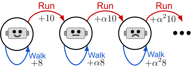
Figure 1: RoboToy domain.

Consider a robot that can perform a task each day either by ‘walking’ or ‘running’. A reward of $8$ is obtained upon completion using ‘walking’, but ‘running’ finishes the task quickly and results in a reward of $10$. However, ‘running’ wears out the motors, thereby increasing the time to finish the task the next day and reduces the returns for both ‘walking’ and ‘running’ by a small factor, $\alpha\in(0,1)$.

Here, methods for tackling passive non-stationarity will track the best policy under the assumption that the changes due to damages are because of external factors and would fail to attribute the cause of damage to the agent’s decisions. Therefore, as on any given day ‘running’ will always be better, every day these methods will prefer ‘running’ over ‘walking’ and thus aggravate the damage. Since the outcome on each day is dependent on decisions made during previous days this leads to active non-stationarity, where ‘walking’ is better in the long run. Finding a better policy first requires a method to evaluate a policy’s (future) performance, which is the focus of this work.

Notice that the above problem can also be viewed as a task with effectively a single lifelong episode. However, as we discuss later in Section 4, approaches such as modeling the problem as a large stationary POMDP or as a continuing average-reward MDP with a single episode may not be viable. Further, non-stationarity can also be observed in multi-agent systems and games due to different agents/players interacting with the system. However, often the goal in these other areas is to search for (Nash) equilibria, which may not even exist under hybrid non-stationarity. Non-stationarity may also result due to artifacts of the learning algorithm even when the problem is stationary. While relevant, these other research areas are distinct from our setting of interest and we discuss them and others in more detail in Appendix B.

3 Non-Stationary Decision Processes

We build upon the formulation used by past work (Xie et al., 2020a; Chandak et al., 2020b) and consider that the agent interacts with a lifelong sequence of partially observable Markov decision processes (POMDPs), $(M_{i})_{i=1}^{\infty}$. However, unlike prior problem formulations, we account for active and hybrid non-stationarity by considering POMDP $M_{i+1}$ to be dependent on both on the POMDP $M_{i}$ and the decisions made by the agent while interacting with $M_{i}$. We provide a control graph for this setup in Figure 2. For simplicity of presentation, we will often ignore the dependency of $M_{i+1}$ on $M_{i-k}$ for $k>0$, although our results can be extended for settings with $k>0$.

Notation: Let $\mathcal{M}$ be a finite set of POMDPs. Each POMDP $M_{i}\in\mathcal{M}$ is a tuple $(\mathcal{O},\mathcal{S},\mathcal{A},\Omega_{i},P_{i},R_{i},\mu_{i})$, where $\mathcal{O}$ is the set of observations, $\mathcal{S}$ is the set of states, and $\mathcal{A}$ is the set of actions, which are the same for all the POMDPs in $\mathcal{M}$. For simplicity of notation, we assume $\mathcal{M},\mathcal{S},\mathcal{O},\mathcal{A}$ are finite sets, although our results can be extended to settings where these sets are infinite or continuous. Let $\Omega_{i}:\mathcal{S}\times\mathcal{O}\rightarrow[0,1]$ be the observation function, $P_{i}:\mathcal{S}\times\mathcal{A}\times\mathcal{S}\rightarrow[0,1]$ be the transition function, $\mu_{i}:\mathcal{S}\rightarrow[0,1]$ be the starting state distribution, and $R_{i}:\mathcal{S}\times\mathcal{A}\rightarrow[-R_{\max},R_{\max}]$ be the reward function with $0\leq R_{\max}<\infty$.

Let $\pi:\mathcal{O}\times\mathcal{A}\rightarrow[0,1]$ be any policy and $\Pi$ be the set of all policies. Let $H_{i}\coloneqq(O_{i}^{t},A_{i}^{t},R_{i}^{t})_{t=1}^{T}$ be a sequence of at most $T$ interactions in $M_{i}$, where $O_{i}^{t},A_{i}^{t},R_{i}^{t}$ are the random variables corresponding to the observation, action, and reward at the step $t$. Let $G_{i}\coloneqq\sum_{t=1}^{T}R_{i}^{t}$ be an observed return and $J_{i}(\pi)\coloneqq\mathbb{E}_{\pi}[G_{i}|M_{i}]$ be the performance of $\pi$ on $M_{i}$. Let $\mathcal{H}$ be the set of possible interaction sequences, and finally let $\mathcal{T}:\mathcal{M}\times\mathcal{H}\times\mathcal{M}\rightarrow[0,1]$ be the transition function that governs the non-stationarity in the POMDPs. That is, $\mathcal{T}(m,h,m^{\prime})=\Pr(M_{i+1}{=}m^{\prime}|M_{i}{=}m,H_{i}{=}h)$.

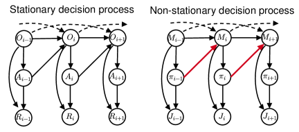
Figure 2: Control Graph for the non-stationary process. See text for symbol definitions.

Figure 2 (Left) depicts the control graph for a stationary POMDP, where each column corresponds to one time step. Here, multiple, independent episodes from the same POMDP can be resampled. (Right) Control graph that we consider for a non-stationary decision process, where each column corresponds to one episode. Here, the agent interacts with a single sequence of related POMDPs $(M_{i})_{i=1}^{n}$. Absence or presence of the red arrows indicates whether the change from $M_{i}$ to $M_{i+1}$ is independent of the decisions in $M_{i}$ (passive non-stationarity) or not (active non-stationarity).

Problem Statement: We look at the fundamental problem of evaluating the performance of a policy $\pi$ in the presence of non-stationarity. Let $(H_{i})_{i=1}^{n}$ be the data collected in the past by interacting using policies $(\beta_{i})_{i=1}^{n}$. Let $D_{n}$ be the dataset consisting of $(H_{i})_{i=1}^{n}$ and the probabilities of the actions taken by $(\beta_{i})_{i=1}^{n}$. Given $D_{n}$, we aim to evaluate the expected future performance of $\pi$ if it is deployed for the next $L$ episodes (each a different POMDP), that is $\mathscr{J}(\pi)\coloneqq\mathbb{E}_{\pi}\left[\sum_{k=n+1}^{n+L}J_{k}(\pi)\middle|(H_{i})_{i=1}^{n}\right].$ We call it the on-policy setting if $\forall i,\beta_{i}=\pi$, and the off-policy setting otherwise. Notice that even in the on-policy setting, naively aggregating observed performances from $(H_{i})_{i=1}^{n}$ may not be indicative of $\mathscr{J}(\pi)$ as $M_{k}$ for $k>n$ may be different than $M\in(M_{i})_{i=1}^{n}$ due to non-stationarity.

4 Understanding Structural Assumptions

A careful reader would have observed that instead of considering interactions with a sequence of POMDPs $(M_{i})_{i=1}^{n}$ that are each dependent on the past POMDPs and decisions, an equivalent setup might have been to consider a ‘chained’ sequence of interactions $(H_{1},H_{2},...,H_{n})$ as a single episode in a ‘mega’ POMDP comprised of all $M\in\mathcal{M}$. Consequently, $\mathscr{J}(\pi)$ would correspond to the expected future return given $(H_{i})_{i=1}^{n}$. Tackling this single long sequence of interactions using the continuing/average-reward setting is not generally viable because methods for these settings rely on an ergodicity assumption (which implies that all states can always be revisited) that may not hold in the presence of non-stationarity. For instance, in the earlier example of automated healthcare, it is not possible to revisit past years.

To address the above challenge, we propose introducing a different structural assumption. Particularly, framing the problem as a sequence of POMDPs allows us to split the single sequence of interactions into multiple (dependent) fragments, with additional structure linking together the fragments. Specifically, we make the following intuitive assumption.

Assumption 1.

ass:fixedf $\forall m\in\mathcal{M}$ such that the performance $J(\pi)$ associated with $m$ is $j$,

$$\forall\pi,\pi^{\prime}\in\Pi^{2},\forall i,\,\Pr(J_{i+1}(\pi)=j_{i+1}|M_{i}=m;\pi^{\prime})=\Pr(J_{i+1}(\pi)=j_{i+1}|J_{i}(\pi)=j;\pi^{\prime}).$$ (1)

ass:fixedf characterizes the probability that $\pi$’s performance will be $j_{i+1}$ in the $i+1^{\text{th}}$ episode when the policy $\pi^{\prime}$ is executed in the $i^{\text{th}}$ episode. To understand ass:fixedf intuitively, consider a ‘meta-transition’ function that characterizes $\Pr(J_{i+1}(\pi)|J_{i}(\pi),\pi^{\prime})$ similar to how the standard transition function in an MDP characterizes $\Pr(S_{t+1}|S_{t},A_{t})$. While the underlying changes actually happen via $\mathcal{T}$, ass:fixedf imposes the following two conditions: (a) A higher-order stationarity condition on the meta-transitions under which non-stationarity can result in changes over time, but the way the changes happen is fixed, and (b) Knowing the past performance(s) of a policy $\pi$ provides sufficient information for the meta-transition function to model how the performance will change upon executing any (possibly different) policy $\pi^{\prime}$. For example, in the earlier toy robot domain, given the current performance there exists an (unknown) oracle that can predict the performance for the next day if the robot decides to ‘run’/‘walk’.

ass:fixedf is beneficial as it implicitly captures the effect of both the underlying passive and active non-stationarity by modeling the conditional distribution of the performance $J_{i+1}(\pi)$ given $J_{i}(\pi)$, when executing any (different) policy $\pi^{\prime}$. At the same time, notice that it generalizes (a) the stationary setting, where $\forall\pi\in\Pi,\,\forall i>0,J_{i+1}(\pi)=J_{i}(\pi)$, and (b) only passive non-stationarity, which is a special case of (1) wherein $\pi^{\prime}$ does not influence the outcome, i.e.,

$$\forall\pi_{a},\pi_{b}\in\Pi^{2},\,\forall i>0,\,\Pr(J_{i+1}(\pi)=J_{i+1}|J_{i}(\pi)=j;{\color[rgb]{1,0,0}\pi_{a}})=\Pr(J_{i+1}(\pi)=J_{i+1}|J_{i}(\pi)=j;{\color[rgb]{1,0,0}\pi_{b}}).$$ (2)

Remark 1.

In some cases, it may be beneficial to relax ass:fixedf such that instead of using $\Pr(J_{i+1}(\pi)|J_{i}(\pi);\pi^{\prime})$ in (1), one considers $\Pr(J_{i+1}(\pi)|(J_{i-k}(\pi))_{k=0}^{p};\pi^{\prime})$. This can be considered similar to the p-Markov MDP where the transitions are characterized using $\Pr(S_{t+1}|(S_{t-i})_{i=0}^{p},A_{t})$. While we consider this general setting for our empirical results, for simplicity, to present the key ideas we will consider (1). We provide a detailed discussion on cases where we expect such an assumption to be (in)valid, and also other potential assumptions in Appendix C. rem:p

5 Model-Free Policy Evaluation

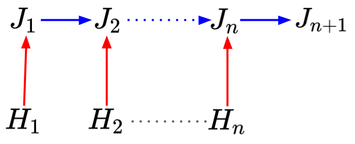
Figure 3: High-level idea.

In this section we discuss how under ass:fixedf, we can perform model-free off-policy evaluation amidst passive, active, or hybrid non-stationarity. The high level idea can be decomposed into the following: (a) Obtain estimates of $(J_{i}(\pi))_{i=1}^{n}$ using $(H_{i})_{i=1}^{n}$ (red arrows in Figure 3), and (b) Use the estimates of $(J_{i}(\pi))_{i=1}^{n}$ to infer the effect of the underlying non-stationarity on the performance, and use that to predict $(J_{i}(\pi))_{i=n+1}^{n+L}$ (blue arrows in Figure 3).

5.1 Counterfactual Reasoning

$(J_{i}(\pi))_{i=1}^{n}$ could have been directly estimated if we had access to $(M_{i})_{i=1}^{n}$. However, how do we estimate $(J_{i}(\pi))_{i=1}^{n}$ when we only have $(H_{i})_{i=1}^{n}$ collected using interactions via possibly different data collecting policies $(\beta_{i})_{i=1}^{n}$?

To estimate $(J_{i}(\pi))_{i=1}^{n}$, we use the collected data $D_{n}$ and aim to answer the following counterfactual question: what would the performance of $\pi$ would have been, if $\pi$ was used to interact with $M_{i}$ instead of $\beta_{i}$? To answer this, we make the following standard support assumption (Thomas et al., 2015; Thomas and Brunskill, 2016; Xie et al., 2019) that says that any action that is likely under $\pi$ is also sufficiently likely under the policy $\beta_{i}$ for all $i$.

Assumption 2.

$\forall o\in\mathcal{O},\forall a\in\mathcal{A}$, and $\forall i\leq n$, $\frac{\pi(o,a)}{\beta_{i}(o,a)}$ is bounded above by a (unknown) constant $c$. ass:support

Under ass:support, an unbiased estimate of $J_{i}(\pi)$ can be obtained using common off-policy evaluation methods like importance sampling (IS) or per-decision importance sampling (PDIS) (Precup, 2000), $\forall i,\widehat{J}_{i}(\pi)\coloneqq\sum_{t=1}^{T}\rho_{i}^{t}R_{i}^{t},\text{ where, }\rho_{i}^{t}\coloneqq\prod_{j=1}^{t}\!\!\frac{\pi(O_{i}^{j},A_{i}^{j})}{\beta_{i}(O_{i}^{j},A_{i}^{j})}.$ This $\widehat{J}_{i}(\pi)$ provides an estimate of $J_{i}(\pi)$ associated with each $M_{i}$ and policy $\pi$, as needed for the red arrows in Figure 3.

5.2 Double Counterfactual Reasoning

Having obtained the estimates for $(J_{i}(\pi))_{i=1}^{n}$, we now aim to estimate how the performance of $\pi$ changes due to the underlying non-stationarity. Recall that under active or hybrid non-stationarity, changes in a policy’s performance due to the underlying non-stationarity is dependent on the past actions. From ass:fixedf, let

$$\forall i>0,\quad F_{\pi}(x,\pi^{\prime},y)\coloneqq\Pr(J_{i+1}(\pi)=y|J_{i}(\pi)=x;\pi^{\prime})$$ (3)

denote how the performance of $\pi$ changes between episodes, if $\pi^{\prime}$ was executed. Here $J_{i+1}(\pi)$ is a random variable because of stochasticity in $H_{i}$ (i.e., how $\pi^{\prime}$ interacts in $M_{i}$), as well as in the meta-transition from POMDP $M_{i}$ to $M_{i+1}$. Similarly, let

$$\forall i>0,\quad f(J_{i}(\pi),\pi^{\prime};\theta_{\pi})\coloneqq\mathbb{E}_{\pi^{\prime}}\left[J_{i+1}(\pi)|J_{i}(\pi)\right]=\sum\nolimits_{y\in\mathbb{R}}F_{\pi}(J_{i}(\pi),\pi^{\prime},y)y$$ (4)

be some (unknown) function parameterized by $\theta_{\pi}\in\Theta$, which denotes the expected performance of $\pi$ in episode $i+1$, if in episode $i$, $\pi$’s performance was $J_{i}(\pi)$ and $\pi^{\prime}$ was executed. Parameters $\theta_{\pi}$ depend on $\pi$ and thus $f$ can model different types of changes to the performance of different policies.

Recall from Figure 3 (blue arrows), if we can estimate $f(\cdot,\pi;\theta_{\pi})$ to infer how $J_{i}(\pi)$ changes due to the underlying non-stationarity when interacting with $\pi$, then we can use it to predict $(J_{i}(\pi))_{i=n+1}^{n+L}$ when $\pi$ is deployed in the future. In the following, we will predominantly focus on estimating $f(\cdot,\pi;\theta_{\pi})$ using past data $D_{n}$. Therefore, for brevity we let $f(\cdot;\theta_{\pi})\coloneqq f(\cdot,\pi;\theta_{\pi})$.

If pairs of $(J_{i}(\pi),J_{i+1}(\pi))$ are available when the transition between $M_{i}$ and $M_{i+1}$ occurs due to execution of $\pi$, then one could auto-regress $J_{i+1}(\pi)$ on $J_{i}(\pi)$ to estimate $f(\cdot;\theta_{\pi})$ and model the changes in the performance of $\pi$. However, the sequence $(\widehat{J}_{i}(\pi))_{i=1}^{n}$ obtained from counterfactual reasoning cannot be used as-is for auto-regression. This is because the changes that occurred between $M_{i}$ and $M_{i+1}$ are associated with the execution of $\beta_{i}$, not $\pi$. For example, recall the toy robot example in Figure 1. If data was collected by mostly ‘running’, then the performance of ‘walking’ would decay as well. Directly auto-regressing on the past performances of ‘walking’ would result in how the performance of ‘walking’ would change when actually executing ‘running’. However, if we want to predict performances of ‘walking’ in the future, what we actually want to estimate is how the performance of ‘walking’ changes if ‘walking’ is actually performed.

To resolve the above issue, we ask another counter-factual question: What would the performance of $\pi$ in $M_{i+1}$ have been had we executed $\pi$, instead of $\beta_{i}$, in $M_{i}$? In the following theorem we show how this question can be answered with a second application of the importance ratio $\rho_{i}\coloneqq\rho_{i}^{T}$.

Theorem 1.

lemma:doubleIS Under ass:fixedf,ass:support, $\forall m\in\mathcal{M}$ such that the performance $J(\pi)$ associated with $m$ is $j$, $\mathbb{E}_{\pi}\left[J_{i+1}(\pi)|J_{i}(\pi)=j\right]=\mathbb{E}_{\beta_{i},\beta_{i+1}}\big{[}\rho_{i}\widehat{J}_{i+1}(\pi)\big{|}M_{i}=m\big{]}$.

See Appendix D.1 for the proof. Intuitively, as $\beta_{i}$ and $\beta_{i+1}$ were used to collect the data in $i$ and $i+1^{\text{th}}$ episodes, respectively, lemma:doubleIS uses $\rho_{i}$ to first correct for the mismatch between $\pi$ and $\beta_{i}$ that influences how $M_{i}$ changes to $M_{i+1}$ due to interactions $H_{i}$. Secondly, $\widehat{J}_{i+1}$ corrects for the mismatch between $\pi$ and $\beta_{i+1}$ for the sequence of interactions $H_{i+1}$ in $M_{i+1}$.

5.3 Importance-Weighted IV-Regression

An important advantage of lemma:doubleIS is that given $J_{i}(\pi)$, $\rho_{i}\widehat{J}_{i+1}(\pi)$ provides an unbiased estimate of $\mathbb{E}_{\pi}\left[J_{i+1}(\pi)|J_{i}(\pi)\right]$, even though $\pi$ may not have been used for data collection. This permits using $Y_{i}\coloneqq\rho_{i}\widehat{J}_{i+1}(\pi)$ as a target for predicting the next performance given $X_{i}\coloneqq J_{i}(\pi)$, i.e., to estimate $f(J_{i}(\pi);\theta_{\pi})$ through regression on $(X_{i},Y_{i})$ pairs.

However, notice that performing regression on the pairs $(X_{i}=J_{i}(\pi),Y_{i}=\rho\widehat{J}_{i+1}(\pi))_{i=1}^{n-1}$ may not be directly possible as we do not have $J_{i}(\pi)$; only unbiased estimates $\widehat{J}_{i}(\pi)$ of $J_{i}(\pi)$. This is problematic because in least-squares regression, while noisy estimates of the target variable $Y_{i}$ are fine, noisy estimates of the input variable $X_{i}$ may result in estimates of $\theta_{\pi}$ that are not even asymptotically consistent even when the underlying $f$ is a linear function of its inputs. To see this clearly, consider the following naive estimator,

$$\hat{\theta}_{\texttt{naive}} \in\operatorname*{argmin}_{\theta\in\Theta}\,\,\sum\nolimits_{i=1}^{n-1}\left(f\left(\widehat{J}_{i}(\pi);\theta\right)-\rho_{i}\widehat{J}_{i+1}(\pi)\right)^{2}.$$ (5)

Because $\widehat{J}_{i}(\pi)$ is an unbiased estimate of $J_{\pi}$, without loss of generality, let $\widehat{J}_{i}(\pi)=J_{i}(\pi)+\eta_{i}$, where $\eta_{i}$ is mean zero noise. Let $\mathbb{N}\coloneqq[\eta_{1},\eta_{2},...,\eta_{n-1}]^{\top}$ and $\mathbb{J}\coloneqq[J_{1}(\pi),J_{2}(\pi),...,J_{n-1}(\pi)]^{\top}$. $\theta_{\texttt{naive}}$ can now be expressed as (see Appendix D.2),

$$\hat{\theta}_{\texttt{naive}}\overset{a.s.}{\longrightarrow}\left(\mathbb{J}^{\top}\mathbb{J}+\mathbb{N}^{\top}\mathbb{N}\right)^{-1}\mathbb{J}^{\top}\mathbb{J}\theta_{\pi}\,\,\cancel{\overset{a.s.}{\longrightarrow}}\,\theta_{\pi}.$$ (6)

Observe that $\mathbb{N}^{\top}\mathbb{N}$ in (6) relates to the variances of the mean zero noise variables $\eta_{i}$. The greater the variances, the more $\hat{\theta}_{\texttt{naive}}$ would be biased towards zero (if $\forall i,\,\eta_{i}=0$, then the true $\theta_{\pi}$ is trivially recovered). Intuitively, when the variance of $\eta_{i}$ is high, noise dominates and the structure in the data gets suppressed even in the large-sample regime. Unfortunately, the importance sampling based estimator $\widehat{J}_{i}(\pi)$ in the sequential decision making setting is infamous for extremely high variance (Thomas et al., 2015). Therefore, $\hat{\theta}_{\texttt{naive}}$ can be extremely biased and will not be able to capture the trend in how performances are changing, even in the limit of infinite data and linear $f$. The problem may be exacerbated when $f$ is non-linear.

5.3.1 Bias Reduction

To mitigate the bias stemming from noise in input variables, we introduce a novel instrument variable (IV) (Pearl et al., 2000) regression method for tackling non-stationarity. Instrument variables $Z$ represent some side-information and were originally used in the causal literature to mitigate any bias resulting due to spurious correlation, caused by unobserved confounders, between the input and the target variables. For mitigating bias in our setting, IVs can intuitively be considered as some side-information to ‘denoise’ the input variable before performing regression. For this IV-regression, an ideal IV is correlated with the input variables (e.g., $\widehat{J}_{i}(\pi)$) but uncorrelated with the noises in the input variable (e.g., $\eta_{i}$).

We propose leveraging statistics based on past performances as an IV for $\widehat{J}_{i}(\pi)$. For instance, using $Z_{i}\coloneqq\widehat{J}_{i-1}(\pi)$ as an IV for $\widehat{J}_{i}(\pi)$. Notice that while correlation between $J_{i-1}(\pi)$ and $J_{i}(\pi)$ can directly imply correlation between $\widehat{J}_{i-1}(\pi)$ and $\widehat{J}_{i}(\pi)$, values of $J_{i-1}(\pi)$ and $J_{i}(\pi)$ are dependent on non-stationarity in the past. Therefore, we make the following assumption, which may easily be satisfied when the consecutive performances do not change arbitrarily.

Assumption 3.

$\forall i,\quad\operatorname{Cov}\big{(}\widehat{J}_{i-1}(\pi),\widehat{J}_{i}(\pi)\big{)}\neq 0$. ass:correlated

However, notice that the noise in $\widehat{J}_{i}(\pi)$ can be dependent on $\widehat{J}_{i-1}(\pi)$. This is because non-stationarity can make $H_{i-1}$ and $H_{i}$ dependent, which are in turn used to estimate $\widehat{J}_{i-1}(\pi)$ and $\widehat{J}_{i}(\pi)$, respectively. Nevertheless, perhaps interestingly, we show that despite not being independent, $\widehat{J}_{i-1}(\pi)$ is uncorrelated with the noise in $\widehat{J}_{i}(\pi)$.

Theorem 2.

Under ass:fixedf,ass:support, $\forall i,\quad\operatorname{Cov}\big{(}\widehat{J}_{i-1}(\pi),\widehat{J}_{i}(\pi)-J_{i}(\pi)\big{)}=0$. thm:cov

See Appendix D.3 for the proof. Finally, as IV regression requires learning an additional function $g\coloneqq\mathbb{R}\rightarrow\mathbb{R}$ parameterized by $\varphi\in\Omega$ (intuitively, think of this as a denoising function), we let $\widehat{J}_{i-1}(\pi)$ be an IV for $\widehat{J}_{i}(\pi)$ and propose the following IV-regression based estimator,

$$\hat{\varphi}_{n} \in\operatorname*{argmin}_{\varphi\in\Omega}\,\,\sum\nolimits_{i=2}^{n}\left(g\left(\widehat{J}_{i-1}(\pi);\varphi\right)-\widehat{J}_{i}(\pi)\right)^{2}$$ (7)

$$\hat{\theta}_{n} \in\operatorname*{argmin}_{\theta\in\Theta}\sum\nolimits_{i=2}^{n-1}\left(f\left(g\left(\widehat{J}_{i-1}(\pi);\hat{\varphi}_{n}\right);\theta\right)-\rho_{i}\widehat{J}_{i+1}(\pi)\right)^{2}\!\!\!.$$ (8)

Theorem 3.

thm:consistent Under ass:fixedf,ass:support,ass:correlated, if $f$ and $g$ are linear functions of their inputs, then $\hat{\theta}_{n}$ is a strongly consistent estimator of $\theta_{\pi}$, i.e., $\hat{\theta}_{n}\overset{\text{a.s.}}{\longrightarrow}\theta_{\pi}$. (See Appendix D.3 for the proof.)

Remark 2.

Other choices of instrument variables $Z_{i}$ (apart from $Z_{i}=\widehat{J}_{i-1}(\pi)$) are also viable. We discuss some alternate choices in Appendix E. These other IVs can be used in (7) and (8) by replacing $\widehat{J}_{i-1}(\pi)$ with the alternative $Z_{i}$.

Remark 3.

As discussed earlier, it may be beneficial to model $J_{i+1}(\pi)$ using $(J_{k}(\pi))_{k=i-p+1}^{i}$ with $p>1$. The proposed estimator can be easily extended by making $f$ dependent on multiple past terms $(X_{k})_{k=i-p+1}^{i}$, where $\forall k,\,X_{k}\coloneqq g((\widehat{J}_{l}(\pi))_{l=k-p}^{k-1};\hat{\phi})$. We discuss this in more detail in Appendix E. The proposed procedure is also related to methods that use lags of the time series as instrument variables (Bellemare et al., 2017; Wilkins, 2018; Wang and Bellemare, 2019). rem:p

Remark 4.

An advantage of the model-free setting is that we only need to consider changes in $J(\pi)$, which is a scalar statistic. For scalar quantities, linear auto-regressive models have been known to be useful in modeling a wide variety of time-series trends. Nonetheless, non-linear functions like RNNs and LSTMs (Hochreiter and Schmidhuber, 1997) may also be leveraged using deep instrument variable methods (Hartford et al., 2017; Bennett et al., 2019; Liu et al., 2020; Xu et al., 2020).

As required for the blue arrows in Figure 3, $f(\cdot;\hat{\theta}_{n})$ can now be used to estimate the expected value $\mathbb{E}_{\pi}\left[J_{i+1}(\pi)|J_{i}(\pi)\right]$ under hybrid non-stationarity. Therefore, using $f(\cdot;\hat{\theta}_{n})$ we can now auto-regressively forecast the future values of $(J_{i}(\pi))_{i=n+1}^{n+L}$ and obtain an estimate for $\mathscr{J}(\pi)$. A complete algorithm for the proposed procedure is provided in Appendix E.1.

5.3.2 Variance Reduction

As discussed earlier, importance sampling results in noisy estimates of $J_{i}(\pi)$. During regression, while high noise in the input variable leads to high bias, high noise in the target variables leads to high variance parameter estimates. Unfortunately, (7) and (8) have target variables containing $\rho_{i}$ (and $\rho_{i+1}$) which depend on the product of importance ratios and can thus result in extremely large values leading to higher variance parameter estimates.

The instrument variable technique helped in mitigating bias. To mitigate variance, we draw inspiration from the reformulation of weighted-importance sampling presented for the stationary setting by Mahmood et al. (2014), and propose the following estimator,

$$\tilde{\varphi}_{n} \in\operatorname*{argmin}_{\varphi\in\Omega}\,\,\sum_{i=2}^{n}\bar{\rho}_{i}\left(g\left(\widehat{J}_{i-1}(\pi);\varphi\right)-G_{i}(\pi)\right)^{2}, \text{where \,\,}\bar{\rho}_{i}\coloneqq\frac{\rho_{i}}{\sum_{j=2}^{n}\rho_{j}}$$ (9)

$$\tilde{\theta}_{n} \in\operatorname*{argmin}_{\theta\in\Theta}\sum_{i=2}^{n-1}\rho_{i}^{\dagger}\left(f\left(g\left(\widehat{J}_{i-1}(\pi);\tilde{\varphi}_{n}\right);\theta\right)-G_{i+1}(\pi)\right)^{2}, \text{where \,\,}\rho_{i}^{\dagger}\coloneqq\frac{\rho_{i}\rho_{i+1}}{\sum_{j=2}^{n-1}\rho_{j}\rho_{j+1}}$$ (10)

where $G_{i}$ is the return observed for $M_{i}$. Intuitively, instead of importance weighting the target, we importance weight the squared error, proportional to how likely that error would be if $\pi$ was used to collect the data. Since dividing by any constant does not affect $\tilde{\varphi}_{n}$ and $\tilde{\theta}_{n}$, the choice of $\bar{\rho}_{i}$ and $\rho_{i}^{\dagger}$ ensures that both $\bar{\rho}_{i}$ and $\rho_{i}^{\dagger}\in[0,1]$, thereby mitigating variance but still providing consistency.

Theorem 4.

thm:wconsistent Under ass:fixedf,ass:support,ass:correlated, if $f$ and $g$ are linear functions of their inputs, then $\tilde{\theta}_{n}$ is a strongly consistent estimator of $\theta_{\pi}$, i.e., $\tilde{\theta}_{n}\overset{\text{a.s.}}{\longrightarrow}\theta_{\pi}$. (See Appendix D.3 for the proof.)

6 Empirical Analysis

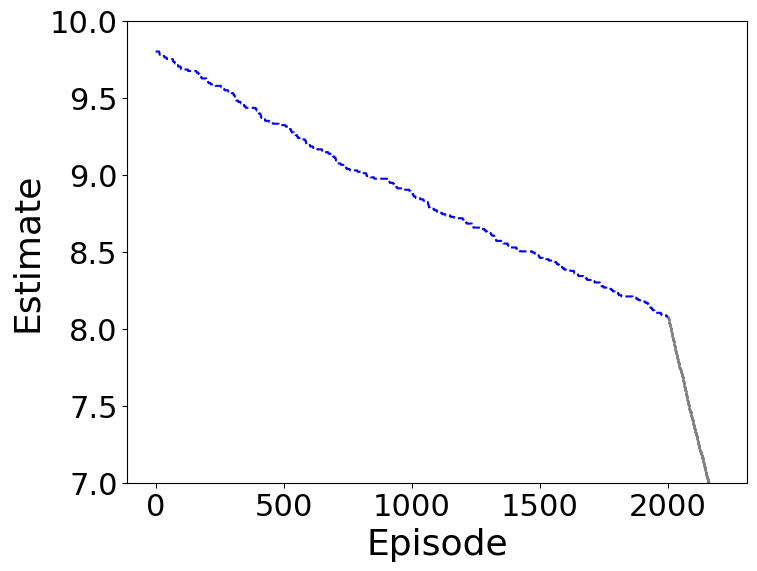
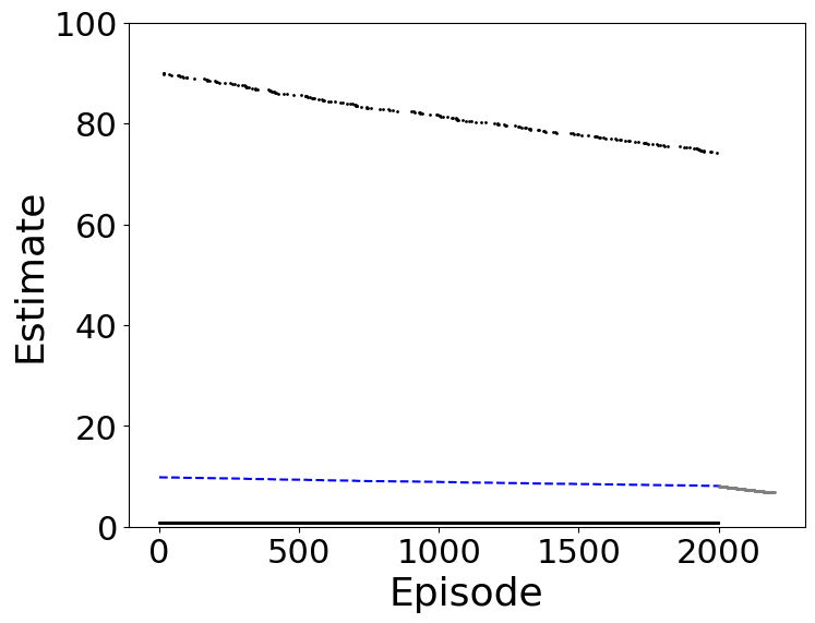
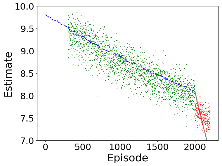
Figure 4: An illustration of the stages in the proposed method for the RoboToy domain of Figure 1. Here, evaluation policy $\pi$ chooses to ‘run’ more often, whereas the data collecting policy $\beta$ chooses to ‘walk’ more often. (Left) This results in a slow decline of performance for $\pi$ initially, followed by a faster decline once $\pi$ is deployed after episode $2000$. The blue and gray curves are unknown to the algorithm. (Middle) OPEN first uses historical data to obtain counterfactual estimates of $J_{i}(\pi)$ for the past episodes. One can see the high-variance in these estimates (notice the change in the y-scale) due to the use of importance sampling. (Right) Intuitively, before naively auto-regressing, OPEN first denoises past performance estimates using the first stage of IV regression (i.e., converts black dots to green dots). It can be observed that OPEN successfully denoises the importance sampling estimates. Using these denoised estimates and a second use of counterfactual reasoning, OPEN performs the second stage of IV regression. It is able to estimate that once $\pi$ is deployed, performances in the future will decrease more rapidly compared to what was observed in the past.

This section presents both qualitative and quantitative empirical evaluations using several environments inspired by real-world applications that exhibit non-stationarity. In the following paragraphs, we first briefly discuss different algorithms being compared and answer three primary questions.

1. OPEN: We call our proposed method OPEN: off-policy evaluation for non-stationary domains with structured passive, active, or hybrid changes. It is based on our bias and variance reduced estimator developed in (9) and (10). Appendix E.1 contains the complete algorithm.

2. Pro-WLS: For the baseline, we use Prognosticator with weighted least-squares (Pro-WLS) (Chandak et al., 2020b). This method is designed to tackle only passive non-stationarity.

3. WIS: A weighted importance sampling based estimator that ignores presence of non-stationarity completely (Precup, 2000).

4. SWIS: Sliding window extension of WIS which instead of considering all the data, only considers data from the recent past.

Q1. (Qualitative Results) What is the impact of the two stages of the OPEN algorithm?

In Figure 4 we present a step by step breakdown of the intermediate stages of a single run of OPEN on the RoboToy domain from Figure 1. It can be observed that OPEN is able to extract the effect of the underlying active non-stationarity on the performances and also detect that the evaluation policy $\pi$ that ‘runs’ more often will cause an active harm, if deployed in the future.

Q2. (Quantitative Results) What is the effect of different types and rates of non-stationarity?

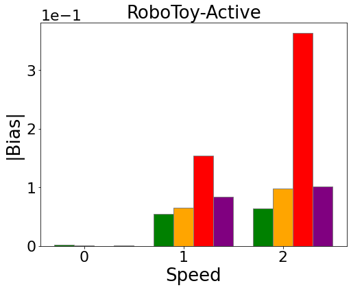
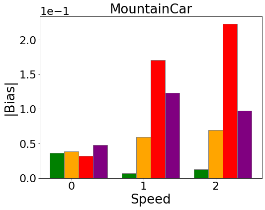
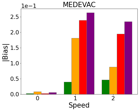
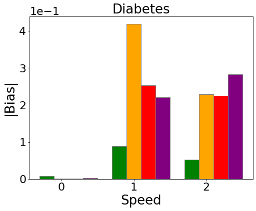
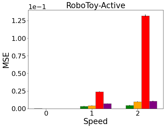
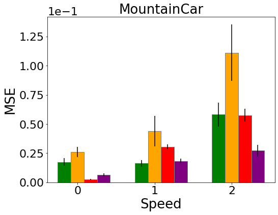
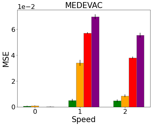
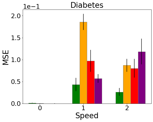
Figure 5: Comparison of different algorithms for predicting the future performance of evaluation policy $\pi$ on domains that exhibit active/hybrid non-stationarity. On the x-axis is the speed which corresponds to the rate of non-stationarity; higher speed indicates faster rate of change and a speed of zero indicates stationary domain. On the y-axes are the absolute bias (Top row) and the mean-squared error (Bottom row) of the predicted performance estimate (lower is better everywhere). For each domain, for each speed, for each algorithm, 30 trials were executed.

Besides the toy robot from Figure 1, we provide empirical results on three other domains inspired by real-world applications that exhibit non-stationarity. Appendix E.3 contains details for each, including how the evaluation policy and the data collecting policy were designed for them.

Non-stationary Mountain Car: In real-world mechanical systems, motors undergo wear and tear over time based on how vigorously they have been used in the past. To simulate similar performance degradation, we adapt the classic (stationary) mountain car domain (Sutton and Barto, 2018). We modify the domain such that after every episode the effective acceleration force is decayed proportional to the average velocity of the car in the current episode. This results in active non-stationarity, where the change in the system is based on the actions taken by the agent in the past.

Type-1 Diabetes Management: Personalised automated healthcare systems for individual patients should account for the physiological and lifestyle changes of the patient over time. To simulate such a scenario we use an open-source implementation (Xie, 2019) of the U.S. Food and Drug Administration (FDA) approved Type-1 Diabetes Mellitus simulator (T1DMS) (Man et al., 2014) for the treatment of Type-1 diabetes, where we induced non-stationarity by oscillating the body parameters (e.g., rate of glucose absorption, insulin sensitivity, etc.) between two known configurations available in the simulator. This induces passive non-stationarity, that is, changes are not dependent on past actions.

MEDEVAC: This domain stands for medical evacuation using air ambulances. This domain was developed by Robbins et al. (2020) for optimally routing air ambulances to provide medical assistance in regions of conflict. Based on real-data, this domain simulates the arrival of different events, from different zones, where each event can have different priority levels. Serving higher priority events yields higher rewards. A good controller decides whether to deploy, and which MEDEVAC to deploy, to serve any event (at the risk of not being able to serve a new high-priority event if all ambulances become occupied). Here, the arrival rates of different events can change based on external incidents during conflict. Similarly, the service completion rate can also change based on how frequently an ambulance is deployed in the past. To simulate such non-stationarity, we oscillate the arrival rate of the incoming high-priority events, which induces passive non-stationarity. Further, to induce wear and tear, we decay the service rate of an ambulance proportional to how frequently the ambulance was used in the past. This induces active non-stationarity. The presence of both active and passive changes makes this domain subject to hybrid non-stationarity.

Figure 5 presents the (absolute) bias and MSE incurred by different algorithms for predicting the future performance of the evaluation policy $\pi$. As expected, the baseline method WIS that ignores the non-stationarity completely fails to capture the change in performances over time. Therefore, while WIS works well for the stationary setting, as the rate of non-stationarity increases, the bias incurred by WIS grows. In comparison, the baseline method Pro-WLS that can only account for passive non-stationarity captures the trend better than WIS, but still performs poorly in comparison to the proposed method OPEN that is explicitly designed to handle active/hybrid non-stationarity. Perhaps interestingly, for the Diabetes domain which only has passive non-stationarity, we observe that OPEN performs better than Pro-WLS. As we discuss later, this can be attributed to the sensitivity of Pro-WLS to its hyper-parameters.

While OPEN incorporated one variance reduction technique, it can be noticed when the rate of non-stationarity is high, variance can sometimes still be high thereby leading to higher MSE. We discuss potential negative impacts of this in Appendix A. Incorporating (partial) knowledge of the underlying model and developing doubly-robust version of OPEN could potentially mitigate variance further. We leave this extension for future work.

Q3. (Ablations Results) How robust are the methods to hyper-parameters?

Due to space constraints, we defer the empirical results and discussion for this to Appendix E.5. Overall, we observe that the proposed method OPEN being an auto-regressive method can extrapolate/forecast better and is thus more robust to hyper-parameters (number of past terms to condition, as discussed in rem:p) than Pro-WLS that uses Fourier bases for regression (where the hyper-parameter is the order of Fourier basis) and is not as good for extrapolation.

7 Conclusion

We took the first steps for addressing the fundamental question of off-policy evaluation under the presence of non-stationarity. Towards this goal we discussed the need for structural assumptions and developed a model-free procedure OPEN and presented ways to mitigate its bias and variance. Empirical results suggests that OPEN can now not only enable practitioners to predict future performances amidst non-stationarity but also identify policies that may be actively causing harm or damage. In the future, OPEN can also be extended to enable control of non-stationary processes.

8 Acknowledgements

Research reported in this paper was sponsored in part by a gift from Adobe, NSF award #2018372. This work was also funded in part by the U.S. Army Combat Capabilities Development Command (DEVCOM) Army Research Laboratory under Cooperative Agreement W911NF-17-2-0196 and Support Agreement No. USMA21050. The views expressed in this paper are those of the authors and do not reflect the official policy or position of the United States Military Academy, the United States Army, the Department of Defense, or the United States Government. The U.S. Government is authorized to reproduce and distribute reprints for Government purposes notwithstanding any copyright notation herein.

Checklist

1. For all authors…

   1. Do the main claims made in the abstract and introduction accurately reflect the paper’s contributions and scope? [Yes]

   2. Did you describe the limitations of your work? [Yes]

   3. Did you discuss any potential negative societal impacts of your work? [Yes]

   4. Have you read the ethics review guidelines and ensured that your paper conforms to them? [Yes]

2. If you are including theoretical results…

   1. Did you state the full set of assumptions of all theoretical results? [Yes]

   2. Did you include complete proofs of all theoretical results? [Yes]

3. If you ran experiments…

   1. Did you include the code, data, and instructions needed to reproduce the main experimental results (either in the supplemental material or as a URL)? [Yes]

   2. Did you specify all the training details (e.g., data splits, hyperparameters, how they were chosen)? [Yes]

   3. Did you report error bars (e.g., with respect to the random seed after running experiments multiple times)? [Yes]

   4. Did you include the total amount of compute and the type of resources used (e.g., type of GPUs, internal cluster, or cloud provider)? [Yes]

4. If you are using existing assets (e.g., code, data, models) or curating/releasing new assets…

   1. If your work uses existing assets, did you cite the creators? [Yes]

   2. Did you mention the license of the assets? [N/A]

   3. Did you include any new assets either in the supplemental material or as a URL? [N/A]

   4. Did you discuss whether and how consent was obtained from people whose data you’re using/curating? [N/A]

   5. Did you discuss whether the data you are using/curating contains personally identifiable information or offensive content? [N/A]

5. If you used crowdsourcing or conducted research with human subjects…

   1. Did you include the full text of instructions given to participants and screenshots, if applicable? [N/A]

   2. Did you describe any potential participant risks, with links to Institutional Review Board (IRB) approvals, if applicable? [N/A]

   3. Did you include the estimated hourly wage paid to participants and the total amount spent on participant compensation? [N/A]

Off-Policy Evaluation for Action-Dependent
Non-Stationary Environments
(Appendix)

.tocmtappendix mtchapternone mtappendixsubsection

Contents

1. 1 Introduction
2. 2 Related Work
3. 3 Non-Stationary Decision Processes
4. 4 Understanding Structural Assumptions
5. 5 Model-Free Policy Evaluation
6. 6 Empirical Analysis
7. 7 Conclusion
8. 8 Acknowledgements
9. A FAQs: Frequently Asked Questions
   1. A.1 How does the stationarity condition for a time-series differ from that in RL?
   2. A.2 Can the POMDP during each episode (Figure 2) itself be non-stationary?
   3. A.3 What if it is known ahead of time that the non-stationarity is passive only?
   4. A.4 How should different non-stationarities be treated in the on-policy setting?
   5. A.5 Can you tell us more about when would ass:fixedf be (in)valid?
   6. A.6 What are the limitations and potential negative impacts of the work?
10. B Extended Related Work
    1. B.1 Off-policy evaluation in stationary domains
    2. B.2 Non-stationarity in stationary domains
    3. B.3 Single Episode Continuing setting
    4. B.4 Non-stationarity in MDPs/Bandits
    5. B.5 Multi-agent Games
    6. B.6 Dynamical Systems and Time-Series Analysis
11. C Discussion on the Structural Assumption
    1. C.1 Latent Variables
12. D Proofs for Theoretical Results
    1. D.1 Double Counterfactual Reasoning
    2. D.2 Asymptotic bias of $\hat{\theta}_{naive}$
    3. D.3 Importance-Weighted IV-Regression
13. E Empirical Details
    1. E.1 Algorithm
    2. E.2 Implementation and Hyper-parameters
    3. E.3 Environments
    4. E.4 Additional Results
       1. E.4.1 Single Run
       2. E.4.2 Summary Plots
    5. E.5 Ablation Study

Appendix A FAQs: Frequently Asked Questions

A.1 How does the stationarity condition for a time-series differ from that in RL?

Conventionally, stationarity is the time-series literature refers to the condition where the distribution (or few moments) of a finite sub-sequence of random-variables in a time-series remains the same as we shift it along the time index axis [Cox and Miller, 2017]. In contrast, the stationarity condition in the RL setting implies that the environment is fixed [Sutton and Barto, 2018]. This makes the performance $J(\pi)$ of any policy $\pi$ to be a constant value throughout. In this work, we use ‘stationarity’ as used in the RL literature.

A.2 Can the POMDP during each episode (Figure 2) itself be non-stationary?

Any source of non-stationarity can be incorporated in the (unobserved) state to induce another stationary POMDP (from which we can obtain a single sequence of interaction). The key step towards tractability is ass:fixedf that enforces additional structure on the performance of any policy across the sequence of (non-)stationary POMDPs.

A.3 What if it is known ahead of time that the non-stationarity is passive only?

In such cases where the underlying changes are independent of the past actions, $\mathbb{E}_{\beta_{1}}[J_{i+1}(\pi)|J_{i}(\pi)]=\mathbb{E}_{\beta_{2}}[J_{i+1}(\pi)|J_{i}(\pi)]$, for any policies $\beta_{1}$ and $\beta_{2}$. Therefore, there is no need for double-counterfactual reasoning to correct for the changes observed in the past. Particularly, in lemma:doubleIS the second use of importance sampling can be avoided as $\mathbb{E}_{\beta_{i},\beta_{i+1}}\left[\rho_{i}\widehat{J}_{i+1}(\pi)\middle|M_{i}(\pi)\right]=\mathbb{E}_{\beta_{i},\beta_{i+1}}\left[\widehat{J}_{i+1}(\pi)\middle|M_{i}(\pi)\right]$ under passive non-stationarity. Rest of the procedure for OPEN can be modified accordingly.

A.4 How should different non-stationarities be treated in the on-policy setting?

Perhaps interestingly, OPEN makes no effective distinction between active and passive non-stationarity in the on-policy setting. Notice that in the on-policy setting, importance ratios $\rho=1$ everywhere, therefore the use of double counterfactual reasoning has no impact. Intuitively, in the on-policy setting, there is no need to dis-entagle the active and passive sources of non-stationarity, as the prediction needs to be made about the same policy that was used during data collection.

A.5 Can you tell us more about when would ass:fixedf be (in)valid?

Yes, we provide a detailed discussion on ass:fixedf in Appendix C.

A.6 What are the limitations and potential negative impacts of the work?

Our work presents the first few steps towards off-policy evaluation in the presence of non-stationarity. Towards this goal, we used ass:fixedf to enforce a higher-order stationarity condition. We have provided extended discussion regarding the same in Appendix C and a practitioner should carefully analyze their problem setup to conclude if the assumption holds (at least approximately).

Further, often off-policy evaluation is used in safety-critical settings, where it is important to provide confidence intervals [Thomas et al., 2015, 2019, Jiang and Huang, 2020]. Because of our use of instrument variables, our estimator may have high-variance. This can be explained by observing the closed form equation in (62) obtained using the IV procedure. Here, $Z$ is the instrument variable and if it is weakly correlated with X (i.e,. $Z^{\top}X$ has a small magnitude) then $(Z^{\top}X)^{-1}$ can be large thereby increasing variance. However, our proposed method OPEN only provides point-estimates and thus using it as-is in safety critical settings would be irresponsible.

If the application does exhibit non-stationarity, a practitioner may have to make a tough choice between prior methods that provide confidence intervals under the stationarity assumption, or the proposed method that may be applicable to their non-stationary setting but does not provide any confidence intervals.

Appendix B Extended Related Work

In this section we discuss several different research directions that are relevant to the topic of this paper. We refer the readers to the work by Padakandla [2020], Khetarpal et al. [2020] for a more exhaustive survey.

B.1 Off-policy evaluation in stationary domains

In the off-policy RL setup, there is a large body of literature that tackles the off-policy estimation problem. One line of work leverages dynamic programming [Puterman, 1990, Sutton and Barto, 2018] to develop off-policy estimators [Boyan, 1999, Sutton et al., 2008, 2009, Mahmood et al., 2014, 2015]. Several recent approaches also build upon a dual perspective for dynamic programming [Puterman, 1990, Wang et al., 2007, Nachum and Dai, 2020] for performing off-policy evaluation [Liu et al., 2018, Xie et al., 2019, Jiang and Huang, 2020, Uehara et al., 2020, Dai et al., 2020, Feng et al., 2021]. These works require fully-observable states. Other direction of work takes Monte-Carlo perspective to perform trajectory based importance sampling and are applicable to stationary setting with partial observability [Precup, 2000, Thomas et al., 2015, Jiang and Li, 2015, Thomas and Brunskill, 2016]. The proposed work builds upon this direction.

Several works have also discussed various techniques for variance reduction [Jiang and Li, 2015, Thomas and Brunskill, 2016, Munos et al., 2016, Harutyunyan et al., 2016, Liu et al., 2018, Espeholt et al., 2018, Nachum et al., 2019, Yang et al., 2020, Yuan et al., 2021]. However, these methods are restricted to stationary domains.

B.2 Non-stationarity in stationary domains

In the face of uncertainty, prior works often opt for exploratory or safe behavior by acting optimistically or pessimistically, respectively. This is often achieved by using the collected data to dynamically modify the observed rewards for any state-action pair by either providing bonuses [Agarwal et al., 2020, Taiga et al., 2021] or penalties [Buckman et al., 2020, Cetin and Celiktutan, 2021]. One could view this as an instance of active non-stationarity. Similarly, in temporal-difference (TD) methods the target for the value function keeps changing and such changes are also dependent on the data collected in the past [Sutton and Barto, 2018]. However, we note that such non-stationarities are only artifacts of the learning algorithm as the underlying domain remains stationary throughout. In contrast, the focus of our work is on settings where the underlying domain is non-stationary.

B.3 Single Episode Continuing setting

As discussed in Section 4, non-stationarity can be alternatively modeled using a single long episode in a stationary POMDP. From this point of view, one may wonder if the average-reward/continuing setting [Sutton and Barto, 2018] could be useful? While there have been off-policy evaluation methods designed to tackle the continuing setting [Liu et al., 2018, Nachum et al., 2019, Yang et al., 2020], they require two important conditions that are no applicable for our setting: (a) They assume access to the true underlying state such that there is no partial-observability, and (b) They assume that the transition tuples are sampled from the stationary state-visitation distribution of a policy. In the non-stationary setting that we consider, we may not have data from any stationary state visitation distribution, and we may not have access to the true underlying states either.

B.4 Non-stationarity in MDPs/Bandits

Several prior methods have considered tackling non-stationarity for reinforcement learning problems. For instance, a Hidden-Mode MDP is a setting that assumes that the environment changes are confined to a few hidden modes, where each mode represents a unique MDP. This provides a tractable way to model a limited number of MDPs [Choi et al., 2000, Basso and Engel, 2009], or perform updates using mode-change detection [Da Silva et al., 2006, Padakandla et al., 2019, Alegre et al., 2021]. Similarly there are methods [Xie et al., 2020a] based on hidden-parameter MDPs [Doshi-Velez and Konidaris, 2016] that consider a more general setup where the hidden variable can be continuous. Alternatively, many methods [Thomas et al., 2017, Jagerman et al., 2019, Chandak et al., 2020b, Zhou et al., 2020, Poiani et al., 2021, Liotet et al., 2021] have considered time-dependent MDPs [Rachelson et al., 2009]. Aspects related to safety and confidence intervals have also been explored [Ammar et al., 2015, Chandak et al., 2020a, 2021]. However, the focus of these methods are on settings with passive non-stationarity, where the past actions do not influence the underlying non-stationarity. Our works extends this direction of research to provide off-policy evaluation amidst active and hybrid non-stationarity as well.

Non-stationary multi-armed bandits (NMAB) capture the setting where the horizon length is one, but the reward distribution changes over time [Moulines, 2008, Besbes et al., 2014, Russac et al., 2019, Vernade et al., 2020]. Many variants of NMAB, like cascading non-stationary bandits [Wang et al., 2019a, Li and de Rijke, 2019] and rotting bandits [Levine et al., 2017, Seznec et al., 2018] have also been considered. In contrast, this work focuses on methods that generalize to the sequential decision making setup where the horizon length can be more than 1.

B.5 Multi-agent Games

Non-stationarity also occurs in multiplayer games [Singh et al., 2000, Bowling, 2005, Conitzer and Sandholm, 2007] where the opponent can change their strategy as a response to the agent’s previous decisions. These types of changes are related to active non-stationarity that we consider in this work. In such games, opponent modeling has been shown to be useful and regret bounds for multi-player games [Zhang and Lesser, 2010, Mealing and Shapiro, 2013, Foster et al., 2016, Foerster et al., 2018]. Further, often these games still assume that the underlying system/environment (excluding other players) is stationary and focus on searching for (Nash) equilibria. Similarly, non-stationarities are also induced in the multi-agent systems where an agent tries to influence other agents [Jaques et al., 2019, Wang et al., 2019b, Xie et al., 2020b, Wang et al., 2021]. However, under general non-stationarity, the underlying system may also change and thus there may not even exist any fixed equilibria. Perhaps a more relevant setting would be that of evolutionary/dynamics games, where the pay-off matrix and specification of the game can change over time [Gemp and Mahadevan, 2017, Hennes et al., 2019]. Such methods, however, do not leverage any underlying structure in how the game is changing nor do they account for settings where the changes might be a consequence of past interactions of the agent. While relevant, these other research areas are distinct from our setting of interest.

B.6 Dynamical Systems and Time-Series Analysis

The proposed method for modeling the evolution of a policy’s performance over time using stochastic estimates of past performances may be reminiscent of state-space methods (e.g., Kalman filtering) for dynamical systems [Hamilton, 1994]. However, in comparison to these methods, we do not need to model noise variables, which could have been challenging in our case as noise is heteroskedastic because of past (off-policy) performance estimates being computed using data from different behavior policies. Further the form of OPEN estimator allows leveraging (accelerated) gradient descent based optimizers to obtain the solution instead of relying on computationally expensive closed-form solutions that are typically needed by state-space models. Due to this, in practice our method can also be used with non-linear functions $f$ (e.g., recurrent neural network based auto-regressive models).

Different applications of time-series analysis have also discussed the use of lags as instruments [Achen, 2000, Reed, 2015, Bellemare et al., 2017, Wilkins, 2018, Wang and Bellemare, 2019]. Our use case differs from these prior works in that we look at the full sequential decision making setup for reinforcement learning, and also consider a novel importance-weighted instrument-variable regression model.

Appendix C Discussion on the Structural Assumption

ass:fixedf states that $\forall m\in\mathcal{M}$ such that the performance $J(\pi)$ associated with $m$ is $j$,

$$\forall i,\,\Pr(J_{i+1}(\pi)=j_{i+1}|M_{i}=m;\pi)=\Pr(J_{i+1}(\pi)=j_{i+1}|J_{i}(\pi)=j;\pi).$$ (11)

As discussed earlier, consider a ‘meta-transition’ function that characterizes $\Pr(J_{i+1}(\pi)|J_{i}(\pi),\pi^{\prime})$ similar to how the standard transition function in an MDP characterizes $\Pr(S_{t+1}|S_{t},A_{t})$. This assumption is imposing the following two conditions: (a) A higher-order stationarity condition on the meta-transitions under which non-stationarity can result in changes over time, but the way the changes happen is fixed, and (b) Knowing the past performance(s) of a policy $\pi$ provides sufficient information for the meta-transition function to model how the performance will change upon executing any (possibly different) policy $\pi^{\prime}$. We provide some examples in Figure 6 to demonstrate few settings to discuss the applicability of this assumption.

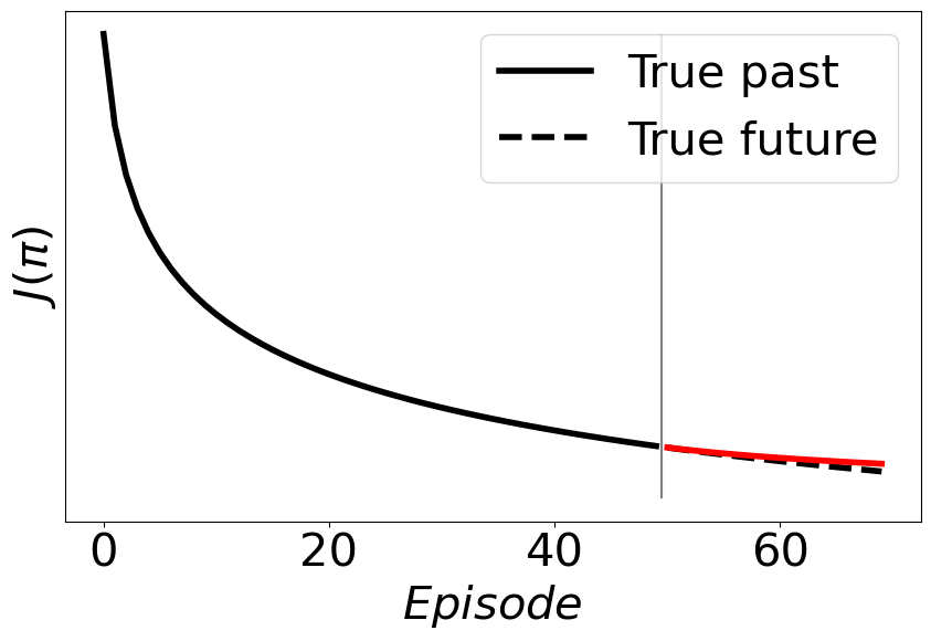
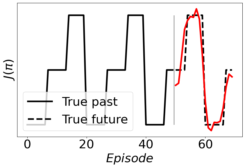
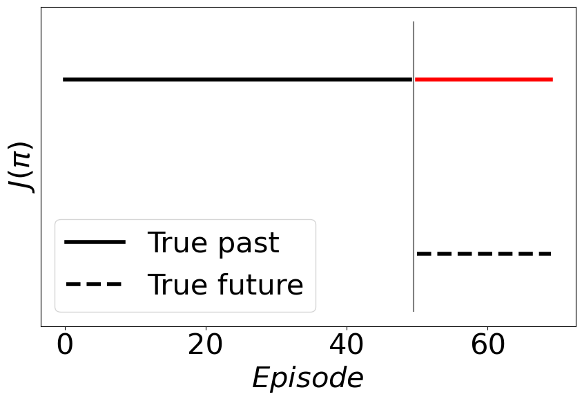
Figure 6: In this figure we plot different kinds of performance trends and discuss the applicability of ass:fixedf for each. The red curve corresponds to the forecast obtained using an auto-regressive model. (Left) In many cases where the performance of a policy is smoothly changing over time (for e.g., drifts in interests of an user that a recommender system needs to account for), looking at the past performances can often provide indication of how the performance would evolve in the future. (Middle) Changes in performances does not necessarily have to be smooth. What ass:fixedf enforces is that the changes have some structure which can be generalized to make predictions about how the performance would change in the future. Here, the performance jumps between different values (for e.g., if there is discontinuous change in the underlying system), but till their is some structure in the changes, it can be leveraged to make predictions about the future performances as well. (Right) While ass:fixedf can be applicable in many setting, there can be settings where this assumption does not hold. For example, if a motor of an industrial system is degrading over time but this degradation has no effect on the observable performance, until the point when the motor breaks down and the performance drops completely. In such cases, just looking at past performances may not be sufficient to infer how performance will change in the future.

C.1 Latent Variables

Instead of enforcing structure on the performances, a possible alternative could have been to enforce structure on how the underlying latent variable (e.g., friction of a motor, interests of a user) are changing over time. While this might be more intuitive for some, just considering structure on this latent variable need not be sufficient. Dealing with latent/hidden variables can particularly challenging in the off-policy setting, as it may often not be possible (unless additional assumptions are enforced) to infer the latent variable using just the observations from past interactions, even in the stationary setting [Tennenholtz et al., 2020, Namkoong et al., 2020, Shi et al., 2021, Bennett et al., 2021].

Further, the end goal is to estimate the performance of a policy in the future. Therefore, even if we could infer the possible latent variables for the future episodes, it would still require additional regularity conditions on the (unknown) function that maps from the latent variable to the performance associated with it for any given policy. Without that it would not be possible to generalize what would the performance be for the inferred latent variables of the future. And as we discuss in Figure 7, these two assumptions on (a) the structure of how the latent variable could change, and (b) the regularity condition on how the latent variable impacts the performance, can often be reduced to a single condition directly on the structure of how the performances are changing.

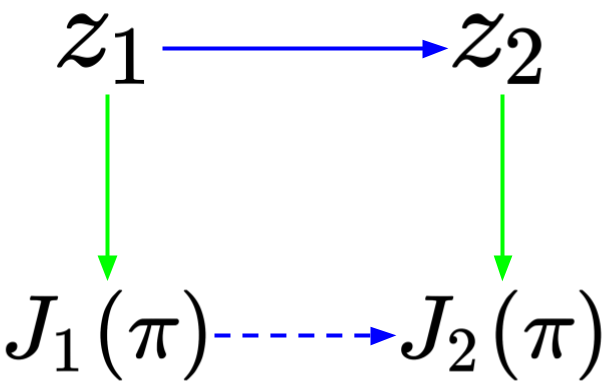
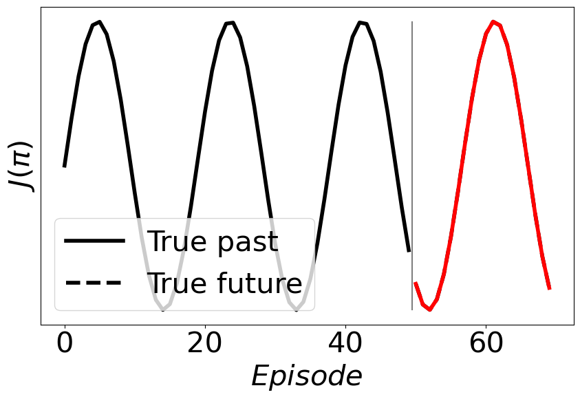
Figure 7: (Left) Considering structured changes in latent variable $z$ (blue arrow) of the POMDP might often be more intuitive. However, as $J(\pi)$ estimation is required ultimately, unless performance of a policy also has some structure (green arrows) given $z$, generalizing across (potentially unseen) $z$’s may not be possible. Structured changes for blue and green arrows consequently results in structured changes in $J(\pi)$ (dashed-blue arrows). For example, if the performance $J(\pi)$ of a policy changes (Lipschitz) smoothly with $z$, then (Lipschitz) smooth changes between $z$ values automatically also imply (Lipschitz) smooth changes between $J(\pi)$ values. (Right) When executing a policy $\pi$, say $z$ changes as $z_{i}=i$, and $J_{i}(\pi)$ changes periodically as $\sin(z_{i})$. Here, even though both $z$ and $J$ change smoothly, changes in $z_{i+1}$ can be modeled using one past term (i.e, $z_{i}$) as given just the current performance value $J_{i}(\pi)$ it is not possible to predict whether the next performance $J_{i+1}(\pi)$ would increase or decrease in the future. However, such a problem can be easily resolved by looking at multiple past performances to infer the trend (for e.g., just using past $2$ terms here suffices to exactly predict the future outcomes(red curve)).

Appendix D Proofs for Theoretical Results

D.1 Double Counterfactual Reasoning

See 1

Proof.

In the following, to make the dependence of trajectories explicit, we will additionally define $\rho(h)$ and $g(h)$ to be the importance ratios and the return associated with a trajectory $h$. Using this notation, it can be observed that,

$$\mathbb{E}_{\pi}\left[J_{i+1}(\pi)|M_{i}\right] =\sum_{h_{i+1}}\Pr(h_{i+1}|M_{i};\pi)g(h_{i+1})$$ (12)

$$\overset{(a)}{=}\sum_{h_{i+1}}\sum_{m_{i+1}}\sum_{h_{i}}\Pr(h_{i+1},m_{i+1},h_{i}|M_{i};\pi)g(h_{i+1})$$ (13)

$$\overset{(b)}{=}\sum_{h_{i}}\Pr(h_{i}|M_{i};\pi)\sum_{m_{i+1}}\Pr(m_{i+1}|h_{i},M_{i};\pi)$$ (14)

$$\quad\quad\sum_{h_{i+1}}\Pr(h_{i+1}|m_{i+1},h_{i},M_{i};\pi)g(h_{i+1})$$ (15)

$$\overset{(c)}{=}\sum_{h_{i}}\Pr(h_{i}|M_{i};\pi)\sum_{m_{i+1}}\Pr(m_{i+1}|h_{i},M_{i})\sum_{h_{i+1}}\Pr(h_{i+1}|m_{i+1};\pi)g(h_{i+1})$$ (16)

$$\overset{(d)}{=}\sum_{h_{i}}\rho(h_{i})\Pr(h_{i}|M_{i};\beta_{k})\sum_{m_{i+1}}\Pr(m_{i+1}|h_{i},M_{i})$$ (17)

$$\quad\quad\sum_{h_{i+1}}\rho(h_{i+1})\Pr(h_{i+1}|m_{i+1};\beta_{i+1})g(h_{i+1})$$ (18)

$$\overset{(e)}{=}\sum_{h_{i}}\sum_{m_{i+1}}\sum_{h_{i+1}}\Pr(h_{i}|M_{i};\beta_{i})\Pr(m_{i+1}|h_{i},M_{i})\Pr(h_{i+1}|m_{i+1};\beta_{i+1})\Big{[}\rho(h_{i})\rho(h_{i+1})g(h_{i+1})\Big{]}$$ (19)

$$=\mathbb{E}_{\beta_{i}\beta_{i+1}}\left[\rho_{i}\rho_{i+1}G_{i+1}|M_{i}\right]$$ (20)

$$=\mathbb{E}_{\beta_{i}\beta_{i+1}}\left[\rho_{i}\widehat{J}_{i+1}(\pi)|M_{i}\right],$$ (21)

where (a) follows from the law of total probability, (b) follows from the chain rule of probability, (c) follows using conditional independence, where $m_{i+1}$ is independent of $\pi$ given $h_{i}$ and $M_{i}$ because of the meta-transition function $\mathcal{T}$, and $h_{i+1}$ i independent of $h_{i}$ and $M_{i}$ given $m_{i+1}$ and $\pi$, (d) follows from the use of importance sampling to switch the sampling distribution under ass:support, and (e) follows from re-arrangement of terms. Finally, $\rho_{i}$ and $\rho_{i+1}$ are the random variables corresponding the importance ratios in episodes $i$ and $i+1$. Random variable $G_{i+1}$ corresponds to the return under $\beta$ in episode $i+1$.

Now notice that

$$\mathbb{E}_{\pi}\left[J_{i+1}(\pi)|M_{i}\right] =\sum_{y\in\mathbb{R}}\Pr(J_{i+1}(\pi)=y|M_{i};\pi)y$$ (22)

$$\overset{(f)}{=}\sum_{y\in\mathbb{R}}\Pr(J_{i+1}(\pi)=y|J_{i}(\pi);\pi)y$$ (23)

$$=\mathbb{E}_{\pi}\left[J_{i+1}(\pi)|J_{i}(\pi)\right],$$ (24)

where $(f)$ follows from ass:fixedf. Finally, combining (21) and (24),

$$\mathbb{E}_{\pi}\left[J_{i+1}(\pi)|J_{i}(\pi)\right]=\mathbb{E}_{\beta_{i},\beta_{i+1}}\left[\rho_{i}\widehat{J}_{i+1}(\pi)\middle|M_{i}\right].$$ (25)

∎

Similarly, under a more generalized ass:fixedf, where $\forall m\in\mathcal{M}$,

$$\forall i>p,\,\Pr(J_{i+1}(\pi)=j_{i+1}|M_{i}=m;\pi^{\prime})=\Pr(J_{i+1}(\pi)=j_{i+1}|(J_{i-k}(\pi)=j_{i-k})_{k=0}^{p};\pi^{\prime}).$$ (26)

then similar steps as earlier can be used to conclude that

$$\mathbb{E}_{\pi}\left[J_{i+1}(\pi)|(J_{i-k}(\pi))_{k=0}^{p}\right] =\mathbb{E}_{\beta_{i}\beta_{i+1}}\left[\rho_{i}\widehat{J}_{i+1}(\pi)|M_{i}\right].$$ (27)

Note that no additional importance correction is needed in (27) compared to (24). The term $\rho_{i}$ only shows up to correct for the transition between $M_{i}$ and $M_{i+1}$ due to the meta-transition function $\mathcal{T}(m,h,m^{\prime})=\Pr(M_{i+1}{=}m^{\prime}|M_{i}{=}m,H_{i}{=}h)$. This independence on the choice of $p$ also holds if $\mathcal{T}$ is non-Markovian in the previous $M_{i}$ values. Although, additional importance correction would be required if $\mathcal{T}$ is dependent on multiple past $H_{i}$ terms.

D.2 Asymptotic bias of $\hat{\theta}_{naive}$

Recall that $\hat{\theta}_{\text{naive}}$ is given by,

$$\hat{\theta}_{\texttt{naive}} \in\operatorname*{argmin}_{\theta\in\Theta}\,\,\sum_{i=1}^{n-1}\left(f\left(\widehat{J}_{i}(\pi);\theta\right)-\rho_{i}\widehat{J}_{i+1}(\pi)\right)^{2}.$$ (28)

Because $\widehat{J}_{i}(\pi)$ is an unbiased estimate of $J_{\pi}$, let $\widehat{J}_{i}(\pi)=J_{i}(\pi)+\eta_{i}$, where $\eta_{i}$ is a mean zero noise. Let $\mathbb{N}\coloneqq[\eta_{1},\eta_{2},...,\eta_{n-1}]^{\top}$ and $\mathbb{J}\coloneqq[J_{1}(\pi),J_{2}(\pi),...,J_{n-1}(\pi)]^{\top}$. When $f$ is a linear function of its inputs, expected value $\mathbb{E}_{\pi}\left[J_{i+1}(\pi)|J_{i}(\pi)\right]=J_{i}\theta_{\pi}$. Also, as $\rho_{i}\hat{J}_{i+1}(\pi)$ is an unbiased estimator for $J_{i}(\pi)\theta_{\pi}$ given $J_{i}(\pi)$, let $\rho_{i}\hat{J}_{i+1}(\pi)=J_{i}(\pi)\theta_{\pi}+\zeta_{i}$, where $\zeta_{i}$ is mean zero noise. Let $\mathbb{N}_{2}\coloneqq[\zeta_{1},\zeta_{2},...,\zeta_{n-1}]^{\top}$ then $\theta_{\texttt{naive}}$ can be expressed as,

$$\hat{\theta}_{\text{naive}} =\left(\left(\mathbb{J}+\mathbb{N}\right)^{\top}\left(\mathbb{J}+\mathbb{N}\right)\right)^{-1}\left(\mathbb{J}+\mathbb{N}\right)^{\top}\left(\mathbb{J}\theta_{\pi}+\mathbb{N}_{2}\right)$$ (29)

$$=\left(\mathbb{J}^{\top}\mathbb{J}+2\mathbb{J}^{\top}\mathbb{N}+\mathbb{N}^{\top}\mathbb{N}\right)^{-1}\left(\mathbb{J}^{\top}\mathbb{J}\theta_{\pi}+\mathbb{N}^{\top}\mathbb{J}\theta_{\pi}+\mathbb{J}^{\top}\mathbb{N}_{2}+\mathbb{N}^{\top}\mathbb{N}_{2}\right)$$ (30)

$$=\left(\frac{1}{n}\left(\mathbb{J}^{\top}\mathbb{J}+2\mathbb{J}^{\top}\mathbb{N}+\mathbb{N}^{\top}\mathbb{N}\right)\right)^{-1}\left(\frac{1}{n}\left(\mathbb{J}^{\top}\mathbb{J}\theta_{\pi}+\mathbb{N}^{\top}\mathbb{J}\theta_{\pi}+\mathbb{J}^{\top}\mathbb{N}_{2}+\mathbb{N}^{\top}\mathbb{N}_{2}\right)\right).$$ (31)

In the limit, using continuous mapping theorem when the inverse in (31) exists,

$$\lim_{n\rightarrow\infty}\hat{\theta}_{\text{naive}} =\left(\lim_{n\rightarrow\infty}\frac{1}{n}\left(\mathbb{J}^{\top}\mathbb{J}+2\mathbb{J}^{\top}\mathbb{N}+\mathbb{N}^{\top}\mathbb{N}\right)\right)^{-1}\left(\lim_{n\rightarrow\infty}\frac{1}{n}\left(\mathbb{J}^{\top}\mathbb{J}\theta_{\pi}+\mathbb{N}^{\top}\mathbb{J}\theta_{\pi}+\mathbb{J}^{\top}\mathbb{N}_{2}+\mathbb{N}^{\top}\mathbb{N}_{2}\right)\right).$$ (32)

Observe that both $\mathbb{N}$ and $\mathbb{N}_{2}$ are mean zero and uncorrelated with each other and also with $\mathbb{J}$. Therefore, the terms corresponding to $\mathbb{J}^{\top}\mathbb{N}$, $\mathbb{J}^{\top}\mathbb{N}_{2}$, and $\mathbb{N}^{\top}\mathbb{N}_{2}$ in (32) will be zero almost surely due to Rajchaman’s strong law of large numbers for uncorrelated random variables [Rajchman, 1932, Chandra, 1991]. However, the term corresponding to $\mathbb{N}^{\top}\mathbb{N}$ will not be zero in the limit, and instead roughly result in (average of the) variances of $\eta_{i}$. Consequently, this results in,

$$\hat{\theta}_{\texttt{naive}}\overset{a.s.}{\longrightarrow}\left(\mathbb{J}^{\top}\mathbb{J}+\mathbb{N}^{\top}\mathbb{N}\right)^{-1}\mathbb{J}^{\top}\mathbb{J}\theta_{\pi}.$$ (33)

D.3 Importance-Weighted IV-Regression

See 2

Proof.

$$\forall i,\,\operatorname{Cov}\left(\widehat{J}_{i}(\pi),\widehat{J}_{i+1}(\pi)-J_{i+1}(\pi)\right) =\underbrace{\mathbb{E}_{\beta}\left[\widehat{J}_{i}(\pi)\left(\widehat{J}_{i+1}(\pi)-J_{i+1}(\pi)\right)\right]}_{\text{(I)}}$$ (34)

$$\quad-\underbrace{\mathbb{E}_{\beta}\left[\widehat{J}_{i}(\pi)\right]\mathbb{E}_{\beta}\left[\widehat{J}_{i+1}(\pi)-J_{i+1}(\pi)\right]}_{\text{(II)}}.$$ (35)

Focusing on term (II),

$$\mathbb{E}_{\beta}\left[\widehat{J}_{i}(\pi)\right]\mathbb{E}_{\beta}\left[\widehat{J}_{i+1}(\pi)-J_{i+1}(\pi)\right] =\mathbb{E}_{\beta}\left[\widehat{J}_{i}(\pi)\right]\left(\mathbb{E}_{\beta}\left[\widehat{J}_{i+1}(\pi)\right]-J_{i+1}(\pi)\right)$$ (36)

$$\overset{(a)}{=}\mathbb{E}_{\beta}\left[\widehat{J}_{i}(\pi)\right]\left(J_{i+1}(\pi)-J_{i+1}(\pi)\right)$$ (37)

$$=0,$$ (38)

where (a) follows from the fact that under ass:support, $\widehat{J}_{i+1}(\pi)$ is an unbiased estimator for $J_{i+1}(\pi)$ [Thomas, 2015]. Focusing on term (I) and using the law of total expectation,

$$\mathbb{E}_{\beta}\left[\widehat{J}_{i}(\pi)\left(\widehat{J}_{i+1}(\pi)-J_{i+1}(\pi)\right)\right] =\mathbb{E}_{\beta}\Big{[}\widehat{J}_{i}(\pi)\underbrace{\mathbb{E}_{\beta}\left[\widehat{J}_{i+1}(\pi)-J_{i+1}(\pi)\middle|\widehat{J}_{i}(\pi)\right]}_{\text{(III)}}\Big{]}.$$ (39)

Expanding term (III) further using the law of total expectation,

$$\mathbb{E}_{\beta}\left[\widehat{J}_{i+1}(\pi)-J_{i+1}(\pi)\middle|\widehat{J}_{i}(\pi)\right] \overset{(b)}{=}\mathbb{E}_{\beta}\left[\mathbb{E}_{\beta}\left[\widehat{J}_{i+1}(\pi)-J_{i+1}(\pi)\middle|M_{i+1},\widehat{J}_{i}(\pi)\right]\middle|\widehat{J}_{i}(\pi)\right]$$ (40)

$$\overset{(c)}{=}\mathbb{E}_{\beta}\left[\mathbb{E}_{\beta}\left[\widehat{J}_{i+1}(\pi)-J_{i+1}(\pi)\middle|M_{i+1}\right]\middle|\widehat{J}_{i}(\pi)\right]$$ (41)

$$\overset{(d)}{=}0,$$ (42)

where in (b) the outer expectation is over the next environment $M_{i+1}$ given that the current performance estimate is $\widehat{J}_{i}(\pi)$ and that $\beta_{i}$ was used for interaction in episode $i$. The inner expectation is over $\widehat{J}_{i+1}(\pi)$, where the trajectory used for estimating $\widehat{J}_{i+1}(\pi)$ is collected using $\beta$ in the environment $M_{i+1}$. Step (c) follows from the fact that conditioned on the environment $M_{i+1}$, interactions in $M_{i+1}$ are independent of quantities observed in the episodes before $i+1$. Finally, step (d) follows from observing that

$$\mathbb{E}_{\beta}\left[\widehat{J}_{i+1}(\pi)-J_{i+1}(\pi)\middle|M_{i+1}\right] =\mathbb{E}_{\beta}\left[\widehat{J}_{i+1}(\pi)\middle|M_{i+1}\right]-J_{i+1}(\pi)$$ (43)

$$\overset{(e)}{=}J_{i+1}(\pi)-J_{i+1}(\pi)$$ (44)

$$=0,$$ (45)

where (e) follows from the fact that under ass:support, $\widehat{J}_{i+1}(\pi)$ is an unbiased estimator of the performance of $\pi$ for the given environment $M_{i+1}$. Therefore both (a) and (b) in (35) are zero, and we conclude the result. ∎

See 3

Proof.

For the linear setting, $\hat{\theta}_{n}$ can be expressed as,

$$\hat{\phi}_{n} \in\operatorname*{argmin}_{\phi\in\Phi}\,\,\sum_{i=2}^{n-1}\left(\widehat{J}_{i-1}(\pi)\phi-\widehat{J}_{i}(\pi)\right)^{2}.$$ (46)

$$\hat{\theta}_{n} \in\operatorname*{argmin}_{\theta\in\Theta}\,\,\sum_{i=2}^{n-1}\left(\bar{J}_{i}(\pi)\theta-\rho_{i}\widehat{J}_{i+1}(\pi)\right)^{2}, \text{where}\quad\bar{J}_{i}\coloneqq\widehat{J}_{i-1}\hat{\phi}_{n}.$$ (47)

Before moving further, we introduce some additional notations. Particularly, we will use matrix based notations such that it provides more insights into how the steps would work out for other choices of instrument variables as well.

$$\bf X_{1} \coloneqq\left[\widehat{J}_{1}(\pi),...,\widehat{J}_{n-2}(\pi)\right]^{\top}, \bf\Lambda_{1} \coloneqq\texttt{diag}([\rho_{1},...,\rho_{n-2}]),$$ (48)

$$\bf X_{2} \coloneqq\left[\widehat{J}_{2}(\pi),...,\widehat{J}_{n-1}(\pi)\right]^{\top}, \bf\Lambda_{2} \coloneqq\texttt{diag}\left(\left[\rho_{2},...,\rho_{n-1}\right]\right),$$ (49)

$$\bf X_{3} \coloneqq\left[\widehat{J}_{3}(\pi),...,\widehat{J}_{n}(\pi)\right]^{\top} \bf\bar{X}_{2} \coloneqq\left[\bar{J}_{2}(\pi),...,\bar{J}_{n-1}(\pi)\right]^{\top},$$ (50)

where the diag corresponds to a diagonal matrix with off-diagonals set to zero.

In the following, we split the proof in two parts: (a) we will first show that

$$\hat{\theta}_{n} =\left(\bf X_{1}^{\top}\bf X_{2}\right)^{-1}\left(\bf X_{1}^{\top}\bf\Lambda_{2}\bf X_{3}\right),$$ (51)

and then (b) using this simplified form for $\hat{\theta}_{n}$ we will show that $\hat{\theta}_{n}\overset{\text{a.s.}}{\longrightarrow}\theta_{\pi}$.

Part (a)

Solving (46) in matrix form,

$$\hat{\phi}_{n} =\left(\bf X_{1}^{\top}\bf X_{1}\right)^{-1}\bf X_{1}^{\top}\bf\bf X_{2}.$$ (52)

Similarly, solving (47) in matrix form,

$$\hat{\theta}_{n} =\left(\bf\bar{X}_{2}^{\top}\bf\bar{X}_{2}\right)^{-1}\bf\bar{X}_{2}^{\top}\bf\Lambda_{2}\bf X_{3}.$$ (53)

Now substituting the value of $\bf\bar{X}_{2}$ in (53),

$$\hat{\theta}_{n} =\left(\left(\underbrace{\bf X_{1}\hat{\phi}_{n}}_{\bf\bar{X}_{2}}\right)^{\top}\left(\underbrace{\bf X_{1}\hat{\phi}_{n}}_{\bf\bar{X}_{2}}\right)\right)^{-1}\left(\underbrace{\bf X_{1}\hat{\phi}_{n}}_{\bf\bar{X}_{2}}\right)^{\top}\bf\Lambda_{2}\bf X_{3}.$$ (54)

Using (52) to substitute the value of $\hat{\phi}_{n}$ in (54),

$$\hat{\theta}_{n} =\left(\left(\bf X_{1}\underbrace{\left(\bf X_{1}^{\top}\bf X_{1}\right)^{-1}\bf X_{1}^{\top}\bf X_{2}}_{\hat{\phi}_{n}}\right)^{\top}\left(\bf X_{1}\underbrace{\left(\bf X_{1}^{\top}\bf X_{1}\right)^{-1}\bf X_{1}^{\top}\bf X_{2}}_{\hat{\phi}_{n}}\right)\right)^{-1}$$ (55)

$$\quad\left(\bf X_{1}\underbrace{\left(\bf X_{1}^{\top}\bf X_{1}\right)^{-1}\bf X_{1}^{\top}\bf X_{2}}_{\hat{\phi}_{n}}\right)^{\top}\bf\Lambda_{2}\bf X_{3}.$$ (56)

Using matrix operations to expand the transposes in (56),

$$\hat{\theta}_{n} =\left(\left(\color[rgb]{1,0,0}\underline{{\color[rgb]{0,0,0}\bf X_{2}^{\top}\bf X_{1}}}\color[rgb]{0,0,0}\left(\color[rgb]{0,0,1}\underline{{\color[rgb]{0,0,0}\bf X_{1}^{\top}\bf X_{1}}}\color[rgb]{0,0,0}\right)^{-1}\color[rgb]{0,1,0}\underline{{\color[rgb]{0,0,0}\bf X_{1}^{\top}}}\color[rgb]{0,0,0}\right)\left(\color[rgb]{0,1,0}\underline{{\color[rgb]{0,0,0}\bf X_{1}}}\color[rgb]{0,0,0}\left(\color[rgb]{.75,0,.25}\underline{{\color[rgb]{0,0,0}\bf X_{1}^{\top}\bf X_{1}}}\color[rgb]{0,0,0}\right)^{-1}\color[rgb]{.75,.5,.25}\underline{{\color[rgb]{0,0,0}\bf X_{1}^{\top}\bf X_{2}}}\color[rgb]{0,0,0}\right)\right)^{-1}$$ (57)

$$\quad\left(\bf X_{2}^{\top}\bf X_{1}\left(\bf X_{1}^{\top}\bf X_{1}\right)^{-1}\bf X_{1}^{\top}\right)\bf\Lambda_{2}\bf X_{3}.$$ (58)

Similarly, using matrix operations to expand inverses in (58) (colored underlines are used to match the terms before expansion in (58) and after expansion in (60)),

$$\hat{\theta}_{n} =\left(\color[rgb]{.75,.5,.25}\underline{{\color[rgb]{0,0,0}\bf X_{1}^{\top}\bf X_{2}}}\color[rgb]{0,0,0}\right)^{-1}\left(\color[rgb]{.75,0,.25}\underline{{\color[rgb]{0,0,0}\bf X_{1}^{\top}\bf X_{1}}}\color[rgb]{0,0,0}\right)\left(\color[rgb]{0,1,0}\underline{{\color[rgb]{0,0,0}\bf X_{1}^{\top}\bf X_{1}}}\color[rgb]{0,0,0}\right)^{-1}\left(\color[rgb]{0,0,1}\underline{{\color[rgb]{0,0,0}\bf X_{1}^{\top}\bf X_{1}}}\color[rgb]{0,0,0}\right)\left(\color[rgb]{1,0,0}\underline{{\color[rgb]{0,0,0}\bf X_{2}^{\top}\bf X_{1}}}\color[rgb]{0,0,0}\right)^{-1}$$ (59)

$$\quad\left(\bf X_{2}^{\top}\bf X_{1}\right)\left(\bf X_{1}^{\top}\bf X_{1}\right)^{-1}\left(\bf X_{1}^{\top}\bf\Lambda_{2}\bf X_{3}\right),$$ (60)

Notice that several terms in (60) cancel each other out, therefore,

$$\hat{\theta}_{n} =\left(\bf X_{1}^{\top}\bf X_{2}\right)^{-1}\left(\bf X_{1}^{\top}\bf\Lambda_{2}\bf X_{3}\right).$$ (61)

As a side remark, we note that if we replace $\bf X_{1}$ in the above steps with an appropriate instrument variable $\bf Z_{1}$, then similar steps will follow and will result in

$$\hat{\theta}_{n} =\left(\bf Z_{1}^{\top}\bf X_{2}\right)^{-1}\left(\bf Z_{1}^{\top}\bf\Lambda_{2}\bf X_{3}\right).$$ (62)

Part (b)

Now when $f(J_{i}(\pi);\theta_{\pi})\coloneqq\mathbb{E}_{\pi}\left[J_{i+1}(\pi)|J_{i}(\pi)\right]$ is a linear function,

$$J_{i+1}(\pi) =J_{i}(\pi)\theta_{\pi}+U_{i+1}(H_{i}),$$ (63)

where $U_{i+1}$ is a bounded mean zero noise (which depends on the interaction $H_{i}$ by $\pi$). Using lemma:doubleIS, let

$$Y_{i+1}\coloneqq\mathbb{E}_{\pi}\left[J_{i+1}(\pi)\middle|J_{i}(\pi)\right]$$

and its unbiased estimate be

$$\widehat{Y}_{i+1}\coloneqq\rho_{i}\widehat{J}_{i+1}(\pi)=\rho_{i}\rho_{i+1}G_{i+1}.$$ (64)

For the regression, since $\widehat{J}_{i}(\pi)$ is an unbiased estimate of the input $J_{i}(\pi)$ and $\widehat{Y}_{i+1}$ is an unbiased estimate of the target $\mathbb{E}_{\pi}\left[J_{i+1}(\pi)\middle|J_{i}(\pi)\right]$, these can be equivalently expressed as,

$$\widehat{J}_{i}(\pi) =J_{i}(\pi)+V_{i}(H_{i}),$$ (65)

$$\widehat{Y}_{i+1} =J_{i+1}(\pi)+W_{i+1}(H_{i},H_{i+1}),$$ (66)

where $V_{i}(H_{i})$ is some bounded mean-zero noise (dependent on the unbiased estimate made using $H_{i}$) and $W_{i+1}(H_{i},H_{i+1})$ is also a bounded mean-zero noise (dependent on the unbiased estimate made using $H_{i}$ and $H_{i+1}$). Before moving further, we define some additional notation,

$$\bf Y_{3} \coloneqq[Y_{3},...,Y_{n}]^{\top} \bf U_{3} \coloneqq[U_{3}(H_{2}),...,U_{n}(H_{n-1})]^{\top},$$ (67)

$$\bf\widehat{Y}_{3} \coloneqq[\widehat{Y}_{3},...,\widehat{Y}_{n}]^{\top} \bf V_{2} \coloneqq[V_{2}(H_{2}),...,V_{n-1}(H_{n-1})]^{\top}.$$ (68)

$$\bf\mathbb{J}_{2} \coloneqq\left[J_{2}(\pi),...,J_{n-1}(\pi)\right]^{\top} \bf W_{3} \coloneqq[W_{3}(H_{2},H_{3}),...,W_{n}(H_{n-1},H_{n})]^{\top}.$$ (69)

Using (64) note that $\bf\widehat{Y}_{3}=\bf\Lambda_{2}\bf X_{3}$, therefore (61) can be expressed as,

$$\hat{\theta}_{n} =\left(\bf X_{1}^{\top}\bf X_{2}\right)^{-1}\left(\bf X_{1}^{\top}\bf\widehat{Y}_{3}\right).$$ (70)

Unrolling value of $\bf\widehat{Y}_{3}$ in (70) using relations from (64) and (66),

$$\hat{\theta}_{n} =\left(\bf X_{1}^{\top}\bf X_{2}\right)^{-1}\left(\bf X_{1}^{\top}\left(\bf Y_{3}+\bf W_{3}\right)\right)$$ (71)

$$=\left(\bf X_{1}^{\top}\bf X_{2}\right)^{-1}\left(\bf X_{1}^{\top}\left(\mathbb{J}_{2}\theta_{\pi}+\bf U_{3}+\bf W_{3}\right)\right)$$ (72)

$$=\left(\bf X_{1}^{\top}\bf X_{2}\right)^{-1}\left(\bf X_{1}^{\top}\left(\left(\bf X_{2}-\bf V_{2}\right)\theta_{\pi}+\bf U_{3}+\bf W_{3}\right)\right).$$ (73)

Expanding (73),

$$\hat{\theta}_{n} =\theta_{\pi}-\left(\bf X_{1}^{\top}\bf X_{2}\right)^{-1}\bf X_{1}^{\top}\bf V_{2}\theta_{\pi}+\left(\bf X_{1}^{\top}\bf X_{2}\right)^{-1}\left(\bf X_{1}^{\top}\left(\bf U_{3}+\bf W_{3}\right)\right).$$ (74)

Evaluating the value of (74) in the limit,

$$\lim_{n\rightarrow\infty}\hat{\theta}_{n}=\theta_{\pi}-\lim_{n\rightarrow\infty}\left(\underbrace{\left(\bf X_{1}^{\top}\bf X_{2}\right)^{-1}\bf X_{1}^{\top}\bf V_{2}\theta_{\pi}}_{(a)}+\underbrace{\left(\bf X_{1}^{\top}\bf X_{2}\right)^{-1}\left(\bf X_{1}^{\top}\left(\bf U_{3}+\bf W_{3}\right)\right)}_{(b)}\right).$$ (75)

It can be now seen from (75) that if in the limit the terms inside the paranthesis are zero, then we would obtain our desired result. Focusing on the term (a) and using the continuous mapping theorem,

$$\lim_{n\rightarrow\infty}\left(\bf X_{1}^{\top}\bf X_{2}\right)^{-1}\bf X_{1}^{\top}\bf V_{2}\theta_{\pi} =\lim_{n\rightarrow\infty}\left(\frac{1}{n}\bf X_{1}^{\top}\bf X_{2}\right)^{-1}\left(\frac{1}{n}\bf X_{1}^{\top}\bf V_{2}\theta_{\pi}\right)$$ (76)

$$=\left(\lim_{n\rightarrow\infty}\frac{1}{n}\bf X_{1}^{\top}\bf X_{2}\right)^{-1}\left(\underbrace{\lim_{n\rightarrow\infty}\frac{1}{n}\bf X_{1}^{\top}\bf V_{2}}_{(c)}\right)\theta_{\pi},$$ (77)

where ass:correlated ensures that $\bf X_{1}$ and $\bf X_{2}$ are correlated and thus their dot product is not zero. Notice that term (c) (77) can be expressed as $\frac{1}{n}\sum_{i=2}^{n-1}X_{i-1}V_{i}$. Further, recall from thm:cov that $V_{i}$ is a mean zero random variable uncorrelated with $X_{i-1}$ for all $i$. Further, $V_{i}$ and $X_{i-1}$ are also bounded for all $i$ as both rewards and importance ratios are bounded (ass:support), and $T$ is finite. Now, for $\alpha_{i}\coloneqq X_{i-1}V_{i}$ observe that $\mathbb{E}\left[\alpha_{i}\right]=\mathbb{E}\left[X_{i-1}\mathbb{E}\left[V_{i}|X_{i-1}\right]\right]=\mathbb{E}\left[X_{i-1}0\right]=0$ and thus $\alpha_{i}$ is a bounded and mean zero random variable $\forall i$. Therefore, as $(c)$ is an average of $\alpha$ variables, it follows from the Rajchaman’s strong law of large numbers for uncorrelated random variables [Rajchman, 1932, Chandra, 1991] that term under $(c)$ is zero almost surely. Thus,

$$\left(\bf X_{1}^{\top}\bf X_{2}\right)^{-1}\bf X_{1}^{\top}\bf V_{2}\theta_{\pi}\overset{\text{a.s.}}{\longrightarrow}0.$$ (78)

Similarly, for term (b) in (75) observe that both $\bf U_{3}$ and $\bf W_{3}$ are zero mean random variables uncorrelated with $\bf X_{1}$. Therefore, term (b) in (75) is also zero in the limit almost surely. It can now be concluded from (75) that

$$\hat{\theta}_{n}\overset{\text{a.s.}}{\longrightarrow}\theta_{\pi}.$$ (79)

∎

See 4

Proof.

For the linear setting, $\tilde{\theta}_{n}$ can be expressed as,

$$\hat{\phi}_{n} \in\operatorname*{argmin}_{\phi\in\Phi}\,\,\sum_{i=2}^{n-1}\rho_{i}\left(\widehat{J}_{i-1}(\pi)\phi-G_{i}(\pi)\right)^{2}.$$ (80)

$$\tilde{\theta}_{n} \in\operatorname*{argmin}_{\theta\in\Theta}\,\,\sum_{i=2}^{n-1}\rho_{i}\rho_{i+1}\left(\bar{J}_{i}(\pi)\theta-G_{i+1}(\pi)\right)^{2}, \text{where}\quad\bar{J}_{i}\coloneqq\widehat{J}_{i-1}\hat{\phi}_{n}.$$ (81)

Notice that as dividing the objective by a positive constant does not change the optima, we drop the denominator terms in

$$\bar{\rho}_{i}\coloneqq\frac{\rho_{i}\rho_{i+1}}{\sum_{j=2}^{n-1}\rho_{j}\rho_{j+1}}$$

for the purpose of the analysis. Before moving further, we introduce some additional notations besides the ones introduced in the proof of thm:consistent,

$$\bf G_{3} \coloneqq\left[G_{3},...,G_{n}\right]^{\top} \bf\bar{\Lambda}_{2} \coloneqq\texttt{diag}\left(\left[\rho_{2}\rho_{3},\rho_{3}\rho_{4}...,\rho_{n-1}\rho_{n}\right]\right),$$ (82)

Solving (80) in matrix form,

$$\hat{\phi}_{n} =\left(\bf X_{1}^{\top}\bf\Lambda_{2}\bf X_{1}\right)^{-1}\bf X_{1}^{\top}\Lambda_{2}\bf G_{2}.$$ (83)

$$=\left(\bf X_{1}^{\top}\bf\Lambda_{2}\bf X_{1}\right)^{-1}\bf X_{1}^{\top}\bf X_{2}.$$ (84)

Similarly, solving (81) in matrix form,

$$\tilde{\theta}_{n} =\left(\bf\bar{X}_{2}^{\top}\bf\bar{\Lambda}_{2}\bf\bar{X}_{2}\right)^{-1}\bf\bar{X}_{2}^{\top}\bf\bar{\Lambda}_{2}\bf G_{3}.$$ (85)

$$\overset{(a)}{=}\left(\bf\bar{X}_{2}^{\top}\bf\bar{\Lambda}_{2}\bf\bar{X}_{2}\right)^{-1}\bf\bar{X}_{2}^{\top}\bf\Lambda_{2}\bf X_{3},$$ (86)

where (a) follows from the fact that $\rho_{i}\rho_{i+1}G_{i+1}=\rho_{i}\widehat{J}_{i+1}(\pi)$. Now substituting the value of $\bf\bar{X}_{2}$ in (86) similar to (54) and (56) in the proof of thm:consistent,

$$\tilde{\theta}_{n} =\left(\left(\color[rgb]{1,0,0}\underline{{\color[rgb]{0,0,0}\bf X_{2}^{\top}\bf X_{1}}}\color[rgb]{0,0,0}\left(\color[rgb]{0,0,1}\underline{{\color[rgb]{0,0,0}\bf X_{1}^{\top}\bf\Lambda_{2}\bf X_{1}}}\color[rgb]{0,0,0}\right)^{-1}\color[rgb]{0,1,0}\underline{{\color[rgb]{0,0,0}\bf X_{1}^{\top}}}\color[rgb]{0,0,0}\right)\color[rgb]{0,1,0}\underline{{\color[rgb]{0,0,0}\bf\bar{\Lambda}_{2}}}\color[rgb]{0,0,0}\left(\color[rgb]{0,1,0}\underline{{\color[rgb]{0,0,0}\bf X_{1}}}\color[rgb]{0,0,0}\left(\color[rgb]{.75,0,.25}\underline{{\color[rgb]{0,0,0}\bf X_{1}^{\top}\bf\Lambda_{2}\bf X_{1}}}\color[rgb]{0,0,0}\right)^{-1}\color[rgb]{.75,.5,.25}\underline{{\color[rgb]{0,0,0}\bf X_{1}^{\top}\bf X_{2}}}\color[rgb]{0,0,0}\right)\right)^{-1}$$ (87)

$$\quad\left(\bf X_{2}^{\top}\bf X_{1}\left(\bf X_{1}^{\top}\bf X_{1}\right)^{-1}\bf X_{1}^{\top}\right)\bf\Lambda_{2}\bf X_{3}.$$ (88)

Similarly, using matrix operations to expand inverses in (88) (colored underlines are used to match the terms before expansion in (88) and after expansion in (90)) and multiplying and dividing by $n$,

$$\tilde{\theta}_{n} =\left(\color[rgb]{.75,.5,.25}\underline{{\color[rgb]{0,0,0}\bf X_{1}^{\top}\bf X_{2}}}\color[rgb]{0,0,0}\right)^{-1}\left(\color[rgb]{.75,0,.25}\underline{{\color[rgb]{0,0,0}\frac{1}{n}\bf X_{1}^{\top}\bf\Lambda_{2}\bf X_{1}}}\color[rgb]{0,0,0}\right)\left(\frac{1}{n}\color[rgb]{0,1,0}\underline{{\color[rgb]{0,0,0}\bf X_{1}^{\top}\bf\bar{\Lambda}_{2}\bf X_{1}}}\color[rgb]{0,0,0}\right)^{-1}\left(\frac{1}{n}\color[rgb]{0,0,1}\underline{{\color[rgb]{0,0,0}\bf X_{1}^{\top}\bf\Lambda_{2}\bf X_{1}}}\color[rgb]{0,0,0}\right)$$ (89)

$$\left(\color[rgb]{1,0,0}\underline{{\color[rgb]{0,0,0}\bf X_{2}^{\top}\bf X_{1}}}\color[rgb]{0,0,0}\right)^{-1}\quad\left(\bf X_{2}^{\top}\bf X_{1}\right)\left(\frac{1}{n}\bf X_{1}^{\top}\bf\Lambda_{2}\bf X_{1}\right)^{-1}\left(\bf X_{1}^{\top}\bf\Lambda_{2}\bf X_{3}\right).$$ (90)

Now focusing on the term underlined in green, in the limit,

$$\lim_{n\rightarrow\infty}\frac{1}{n}\bf X_{1}^{\top}\bf\bar{\Lambda}_{2}\bf X_{1} =\lim_{n\rightarrow\infty}\frac{1}{n}\sum_{i=2}^{n-1}\rho_{i}\rho_{i+1}\widehat{J}_{i-1}(\pi)\widehat{J}_{i-1}(\pi)^{\top}$$ (91)

$$\overset{(a)}{=}\lim_{n\rightarrow\infty}\frac{1}{n}\sum_{i=2}^{n-1}\mathbb{E}_{\beta_{i},\beta_{i+1}}\left[\rho_{i}\rho_{i+1}\right]\widehat{J}_{i-1}(\pi)\widehat{J}_{i-1}(\pi)^{\top}+\frac{1}{n}\sum_{i=2}^{n-1}\varepsilon_{i}\widehat{J}_{i-1}(\pi)\widehat{J}_{i-1}(\pi)^{\top}$$ (92)

$$\overset{(b)}{=}\lim_{n\rightarrow\infty}\frac{1}{n}\sum_{i=2}^{n-1}\widehat{J}_{i-1}(\pi)\widehat{J}_{i-1}(\pi)^{\top}$$ (93)

$$=\lim_{n\rightarrow\infty}\frac{1}{n}\bf X_{1}^{\top}\bf X_{1},$$ (94)

where in (a) we defined random variable $\rho_{i}\rho_{i+1}$ as its expected value $E_{\beta_{i},\beta_{i+1}}\left[\rho_{i}\rho_{i+1}\right]$ plus a mean zero noise $\varepsilon_{i}$. Step (b) follows from first observing that $\rho_{i}$ and $\rho_{i+1}$ are uncorrelated. Therefore $\mathbb{E}_{\beta_{i},\beta_{i+1}}\left[\rho_{i}\rho_{i+1}\right]=\mathbb{E}_{\beta_{i}}\left[\rho_{i}\right]\mathbb{E}_{\beta_{i+1}}\left[\rho_{i+1}\right]=1$ as the expected value of importance ratios is $1$ [Thomas, 2015]. Similarly, $\varepsilon_{i}$ is uncorrelated with $\widehat{J}_{i-1}(\pi)$, i.e., the expected value $\mathbb{E}_{\beta_{i},\beta_{i+1}}\left[\varepsilon_{i}|\widehat{J}_{i-1}(\pi)\right]=\mathbb{E}_{\beta_{i},\beta_{i+1}}\left[\varepsilon_{i}\right]=0$ for any given $J_{i-1}(\pi)$. (Intuitively, this step can be seen analogous to the derivation of PDIS, where the expected value of future IS ratios is always one, irrespective of the past events that it has been conditioned on). Now notice that the random variable $\zeta_{i}\coloneqq\varepsilon_{i}\widehat{J}_{i-1}(\pi)\widehat{J}_{i-1}(\pi)^{\top}$ is bounded and has mean zero for all $i$. Therefore, while $\zeta_{i}$ and $\zeta_{j}$ may be dependent, they are uncorrelated for all $i\neq j$. Using strong law of large number for uncorrelated random variables [Rajchman, 1932, Chandra, 1991] the second term in (a) is zero almost surely.

Similarly, it can be observed that $\frac{1}{n}\bf X_{1}^{\top}\bf\Lambda_{2}\bf X_{1}$ converges to $\frac{1}{n}\bf X_{1}^{\top}\bf X_{1}$. Therefore using (94) in (90), and using the continuous mapping theorem,

$$\tilde{\theta}_{n} \overset{a.s.}{\longrightarrow}\left(\color[rgb]{.75,.5,.25}\underline{{\color[rgb]{0,0,0}\bf X_{1}^{\top}\bf X_{2}}}\color[rgb]{0,0,0}\right)^{-1}\left(\color[rgb]{.75,0,.25}\underline{{\color[rgb]{0,0,0}\frac{1}{n}\bf X_{1}^{\top}\bf X_{1}}}\color[rgb]{0,0,0}\right)\left(\frac{1}{n}\color[rgb]{0,1,0}\underline{{\color[rgb]{0,0,0}\bf X_{1}^{\top}\bf X_{1}}}\color[rgb]{0,0,0}\right)^{-1}\left(\frac{1}{n}\color[rgb]{0,0,1}\underline{{\color[rgb]{0,0,0}\bf X_{1}^{\top}\bf X_{1}}}\color[rgb]{0,0,0}\right)\left(\color[rgb]{1,0,0}\underline{{\color[rgb]{0,0,0}\bf X_{2}^{\top}\bf X_{1}}}\color[rgb]{0,0,0}\right)^{-1}$$ (95)

$$\quad\left(\bf X_{2}^{\top}\bf X_{1}\right)\left(\frac{1}{n}\bf X_{1}^{\top}\bf X_{1}\right)^{-1}\left(\bf X_{1}^{\top}\bf\Lambda_{2}\bf X_{3}\right).$$ (96)

Notice that ass:correlated ensures that $\bf X_{1}$ and $\bf X_{2}$ are correlated and thus their dot product is not zero. Further, several terms in (96) cancel each other out, therefore,

$$\tilde{\theta}_{n} \overset{a.s.}{\longrightarrow}\left(\bf X_{1}^{\top}\bf X_{2}\right)^{-1}\left(\bf X_{1}^{\top}\bf\Lambda_{2}\bf X_{3}\right).$$ (97)

Now proof can be completed similarly to the part (b) of the proof of thm:consistent. ∎

Appendix E Empirical Details

The code for all the algorithms and experiments can be found here https://github.com/yashchandak/activeNS

E.1 Algorithm

In Section 5 we established the key insight for how to forecast the next performance based on a single previous performance, when the true performance trend of a policy can be modeled auto-regressively using a single past term. However, as noted in rem:p and Figure 7 using more terms can provide more flexibility in the the type of trends that can be modeled. Therefore, we leverage statistics based on multiple past terms to form the instrument variable $Z_{i}$.

One immediate choice for $Z_{i}$ is $\widehat{J}_{i}(\pi)$. However, we found that the high variance of IS estimate makes $\widehat{J}_{i}(\pi)$ a weak instrument variable [Pearl et al., 2000], that is not strongly correlated with $J_{i+1}(\pi)$. Better choices of $Z_{i}$ may be the ones that are strongly correlated with $J_{i+1}(\pi)$ but uncorrelated with the noise in the $\widehat{J}_{i+1}(\pi)$ estimate. We found that an alternate choice of $Z_{i}$ composed of the unweighted return $G_{i}$ and a WIS-like estimate for $J_{i}(\pi)$ (where the normalization is done only using the importance ratios from episodes before $i$) to be more useful. Specifically, we let $Z_{i}\coloneqq[G_{i},\widetilde{J}_{i}(\pi)]$, where

$$\widetilde{J}_{i}(\pi)\coloneqq\frac{\rho_{i}G_{i}}{\frac{n}{i}\sum_{k=1}^{i}\rho_{k}}.$$ (98)

It can be observed similar to thm:cov that this $Z_{i}$ is uncorrelated with the noise in $\widehat{J}_{i+1}(\pi)$ as well. Further, the weighted version $\widetilde{J}_{i}(\pi)$ suffers less from variance and we found it to be more strongly correlated with $J_{i+1}(\pi)$. Further, often the performance of the behavior policy is positively/negatively correlated with the performance of the evaluation policy and thus $G_{i}$ tends to be correlated with $J_{i+1}(\pi)$ as well. One could also explore other potential IVs; we leave this for future work.

Now using past $p$ values of $Z_{i}$ to form the complete instrument variable, where $p$ is a hyper-parameter, we use the following importance weighted instrument-variable regression,

$$\tilde{\varphi}_{n} \in\operatorname*{argmin}_{\varphi\in\Omega}\,\,\sum_{i={p+1}}^{n}\bar{\rho}_{i}\left(g\left(\left(Z_{j}(\pi)\right)_{j=i-p}^{i-1};\varphi\right)-G_{i}(\pi)\right)^{2},$$ (99)

$$\tilde{\theta}_{n} \in\operatorname*{argmin}_{\theta\in\Theta}\sum_{i=2p}^{n-1}\rho_{i}^{\dagger}\left(f\left(\left(\bar{J}_{j}(\pi)\right)_{j=i-p+1}^{i};\theta\right)-G_{i+1}(\pi)\right)^{2},$$ (100)

where,

$$\bar{J}_{i}(\pi)= g\left(\left(Z_{j}(\pi)\right)_{j=i-p}^{i-1};\tilde{\varphi}_{n}\right),\quad\forall p<i\leq n,$$ (101)

$$\bar{\rho}_{i}\coloneqq \frac{\rho_{i}}{(\sum_{j=2}^{n}\rho_{j})}\quad$$ (102)

$$\rho_{i}^{\dagger}\coloneqq \frac{\rho_{i}\rho_{i+1}}{(\sum_{j=2}^{n-1}\rho_{j}\rho_{j+1})}.$$ (103)

Once $\tilde{\theta}_{n}$ is obtained, we use it to auto-regressively forecast the future performances. Particularly, we use $(\bar{J}_{k})_{k=n+1}^{n+L}$ as the predicted performances for the next $L$ episodes, where

$$\forall i>n,\,\bar{J}_{i}\coloneqq f\left(\left(\bar{J}_{i-k}(\pi)\right)_{k=1}^{p};\tilde{\theta}_{n}\right).$$ (104)

While our theoretical results were established for the setting where there is only a single regressor ($p=1$), a more generalized theoretical result for $p>1$ may be possible using the concepts of endogenous and exogenous regressors. Particularly, let $[...,X_{i},X_{i+1},X_{i+2},X_{i+3},...]$, be observations from an $AR(2)$ time-series sequence where $X_{i+3}$ depends on $X_{i+1}$ and $X_{i+2}$. Here, using $X_{i+1}$ as the only instrument variable for $X_{i+2}$ is not possible as $X_{i+3}$ is correlated with $X_{i+1}$. However, $Z=X_{i}$ or even $Z=[X_{i},X_{i+1}]$ may form a valid instrument for $X_{i+2}$ as neither the noise in $X_{i+3}$ nor the noise in $X_{i+2}$ is correlated with at least one component of $Z$, i.e., $X_{i}$. For precise instrument relevance conditions and additional discussion, we refer the reader to the works by Abbott [2007], Cameron [2019], Parker [2020]. We leave this theoretical extension for the future work.

E.2 Implementation and Hyper-parameters

For the Pro-WLS baseline, we use the weighted least-squares procedure using the Fourier basis features [Chandak et al., 2020b]. The hyper-parameter for this baseline is the number of Fourier terms $d$ that should be used to estimate the performance trend. We found that setting $d$ to be too high results in extremely high-variance and setting it to a lower value fails to capture the trend in performance. Therefore, based on ablation studies in Figure 10 we set $d=5$ for all the experiments.

WIS estimator uses all the data form the past. In comparison, for sliding windows WIS (SWIS), we set the sliding window length to be $400$ ($20\%$ of the number of episodes in the data) for all the experiments. That is, SWIS use past $400$ episodes to estimate the future performance.

For OPEN, the hyper-parameter corresponds to the number of terms to condition on during auto-regression. Similar to SWIS, we set $p=400$ ($20\%$ of the number of episodes in the data) for all the experiments. That is the AR estimator uses past $400$ episodes to predict the performance in the next episode. For the two stage regression, we observed that choice of learning rate, and avoiding over-fitting (using early-stopping) to be important as well.

For each environment, we collect data consisting of $2000$ episodes of interaction using the behavior policy, and predict the expected future returns if executing the evaluation policy for the next $200$ episodes. The behavior policy and the evaluation policy for each domain are described in Section E.3.

Since the future outcomes are stochastic, to evaluate the true expected future performance in (3), we create digital-clones of the environment after data has been collected using the behavior policy. Using these clones, we compute the average of $30$ possible futures when executing the evaluation policy. This estimate of the expected future returns are then used as the ground truth for comparison with the predictions made by the algorithms.

For Figure 5, $|\text{bias}|$ was computed using the absolute value of the difference between (a) the predicted future performance averaged across 30 trials and (b) the ground truth future performance. That is, for an estimator $\hat{J}$ of $J$, the bias is $|J-E[\hat{J}]|$. Because of this, $30$ trials only gives us a point estimate for bias. (Notice that using the absolute value of the difference between (a) the predicted future performance for each trial and (b) the true future performance’, averaged across $30$ trials, will provide an estimate of $E[|J-\hat{J}|]$, which would not capture the bias but will be more like the variance (using L1/absolute distance instead of L2)).

E.3 Environments

We provide empirical results on four non-stationary environments: a toy robot environment, non-stationary mountain car, diabetes treatment, and MEDEVAC domain for routing air ambulances. Details for each of these environments are provided in this section. For all of the above environments, we regulate the ‘speed’ of non-stationarity to characterize an algorithms’ ability to adapt. Higher speed corresponds to a faster rate of non-stationarity; A speed of zero indicates that the environment is stationary.

RoboToy:

This domain corresponds to the toy robot scenario depicted in Figure 1. Here, a robot can accomplish a task using either by ‘running’ or ‘walking’. Robot finishes a task faster when ‘running’ than ‘walking’ and thus the reward received at the end of ’running’ is higher. However, ‘running’ causes more wear and tear on the robot, thereby degrading the performance of both ‘running’ or ‘walking’ in the future. Since the past interactions influence the non-stationarity, this is an instance of active non-stationarity.

To perform more ablations on our algorithms, we also simulated a RoboToy-Passive domain, where there is no active non-stationarity as above. Instead, the reward obtained at the end of executing the options ‘walking’ or ‘running’ fluctuate across episodes. Therefore, the changes to the underlying system are independent of the actions taken by the agent in the past.

For both the active and passive version of this domain, we collect data using a behavior policy that chooses ‘walking’ more frequently, and the evaluation policy is designed such that it chooses ‘running’ more frequently.

Non-stationary Mountain Car:

In real-world mechanical systems, motors undergo wear and tear over time based on how vigorously they have been used in the past. To simulate similar performance degradation, we adapt the classic (stationary) mountain car domain [Moore, 1990]. We modify the domain such that at every episode the effective acceleration force is decayed proportional to the average velocity of the car in the previous episode. This results in active non-stationarity as the change in the system is based on the actions taken by the agent in the past. Similar to the works by [Thomas, 2015, Jiang and Li, 2015], we make use of macro-actions to repeat an action 10 times, which helps in reducing the effective horizon length of each episode. The maximum number of step per episode using these macros is 30.

For our experiments, using an actor-critic algorithm [Sutton and Barto, 2018] we find a near-optimal policy $\pi$ on the stationary version of the mountain car domain, which we use as the evaluation policy. Let $\pi^{\texttt{rand}}$ be a random policy with uniform distribution over the actions. Then we define the behavior policy $\beta(o,a)\coloneqq 0.5\pi(o,a)+0.5\pi^{\texttt{rand}}(o,a)$ for all states and actions.

Type-1 Diabetes Management:

Automated healthcare systems that aim to personalise for individual patients should account for the physiological changes of the patient over time. To simulate such a scenario we use an open-source implementation [Xie, 2019] of the U.S. Food and Drug Administration (FDA) approved Type-1 Diabetes Mellitus simulator (T1DMS) [Man et al., 2014] for the treatment of Type-1 diabetes, where we induced non-stationarity by oscillating the body parameters (e.g., rate of glucose absorption, insulin sensitivity, etc.) between two known configurations available in the simulator. This induces passive non-stationarity, that is, changes are not dependent on past actions.

Each step of an episode corresponds to a minute ($1440$ timesteps–one for each minute in a day) in an in-silico patient’s body and state transitions are governed by a continuous time non-linear ordinary differential equation (ODE) [Man et al., 2014]. This makes the problem particularly challenging as it is unclear how the performance trends of policies vary in this domain when the physiological parameters of the patient are changed. Notice that as the parameters that are being oscillated are inputs to a non-linear ODE system, the exact trend of performance for any policy is unknown. This more closely reflects a real-world setting where ass:fixedf might not hold, as every policy’s performance trend in real-world problems cannot be expected to follow any specific trend exactly–one can only hope to obtain a coarse approximation of the trend.

For our experiments, using an actor-critic algorithm [Sutton and Barto, 2018] we find a near-optimal policy $\pi$ on the stationary version of this domain, which we use as the evaluation policy. The policy learns the CR and CF parameters of a basal-bolus controller. Let $\pi^{\texttt{rand}}$ be a random policy with uniform distribution over actions. Then we define the behavior policy $\beta(o,a)\coloneqq 0.5\pi(o,a)+0.5\pi^{\texttt{rand}}(o,a)$ for all states and actions.

MEDEVAC:

This domain stands for medical evacuation using air ambulances. This domain was developed by Robbins et al. [2020] for optimally routing air ambulances to provide medical assistance in regions of conflict. This domain divides the region of conflict into $34$ mutually exclusive zones, and has $4$ air ambulances to serve all zones when an event occurs. Based on real-data, this domain simulates the arrival of different events, from different zones, where each event can have $3$ different priority levels. Serving higher priority events yields higher rewards. If an ambulance is assigned to an event, it will finish the assignment in a time dependent on the distance between the base of the ambulance and the zone of the corresponding event. While engaged in an assignment, that ambulance is no longer available to serve other events. A good controller decides whether to deploy, and which MEDEVAC to deploy, to serve any event (at the risk of not being able to serve a new high-priority event if all ambulances become occupied).

The original implementation of the domain assumes that the arrival rates of the events and the time taken by an ambulance to complete an event follow a Poisson process with a fixed rate. However, in reality, the arrival rates of different events can change based on external incidents during conflict. Similarly, the completion rate can also change based on how frequently an ambulance is deployed. To simulate such non-stationarity, we oscillate the arrival rate of the incoming high-priority events, which induces passive non-stationarity. Further, to induce wear and tear, we slowly decay the rate at which an ambulance can finish an assignment. This decay is proportional to how frequently the ambulance was used in the past. This induces active non-stationarity. The presence of both active and passive changes makes this domain subject to hybrid non-stationarity.

Similar to other domains, we used an actor-critic algorithm [Sutton and Barto, 2018] we find a near-optimal policy $\pi$ on the stationary version of this domain, which we use as the evaluation policy. Let $\pi^{\texttt{rand}}$ be a random policy with uniform distribution over the actions. Then we define the behavior policy $\beta(o,a)\coloneqq 0.5\pi(o,a)+0.5\pi^{\texttt{rand}}(o,a)$ for all states and actions.

E.4 Additional Results

While the primary focus of this chapter was to develop methods to handle active/hybrid non-stationarity, we observed that the proposed method OPEN also provides benefits over the earlier algorithm Pro-WLS even when it is known that there is only passive non-stationarity in the environment.

E.4.1 Single Run

Similar to Figure 4, in Figure 8 we present a step by step breakdown of the intermediate stages of a single run of OPEN on the RoboToy-Passive domain. Here the trend in how the performance of the evaluation policy was changing in the past remains the same in the future. When only passive non-stationarity is present, the double counter-factual correction performed by OPEN is superfluous. However, it can be observed that OPEN can still correctly identify the trend and provide useful predictions of $\pi$’s future performance.

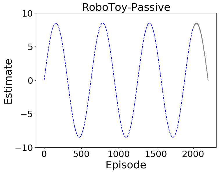
The blue curve corresponds to the performances $J_{i}(\pi)$ for the past episodes. As there is no active non-stationarity, the choice of actions executed does not impact the underlying non-stationarity. Therefore, $J_{i}(\pi)$ follows the same trend in future as it did in the past. The blue and gray curves are unknown to the algorithm.

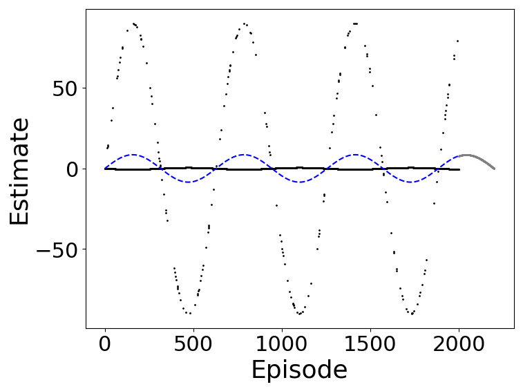
OPEN first uses historical data to obtain counterfactual estimates of $J_{i}(\pi)$ for the past episodes. One can see the high-variance in these estimates (notice the change in the y-scale) due to the use of importance sampling.

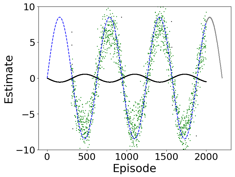
Before naively auto-regressing, OPEN first aims to denoise the past performance estimates using the first stage of instrument variable regression. Since $p=300$, the first $300$ terms were not denoised. It can be observed that OPEN successfully denoises the importance sampling estimates.

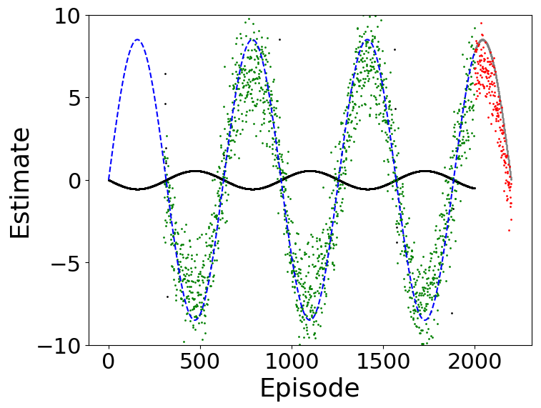
Using the denoised estimates of past performances, with the second use of counterfactual reasoning, OPEN performs the second stage of regression to forecast the future performance when $\pi$ will be deployed. In the passive setting, use of double-counterfactual is superfluous but OPEN is still able to correctly predict the future performance.

Figure 8: An illustrative step by step breakdown of the stages in the proposed algorithm OPEN for the RoboToy-Passive domain.

E.4.2 Summary Plots

In Figure 9 we provide bias and MSE analysis of different algorithms on the domains that exhibit passive non-stationarity. Except for the stationary setting, where WIS has the best performance overall, we observe that for all other settings in the plot, OPEN performs better than both Pro-WLS and WIS consistently.

One thing that particularly stands out in these plots is the poor performance of Pro-WLS, despite being designed for the passive setting. We observed that because of the choice of parametric regression using the Fourier basis, Pro-WLS tends to suffer from high bias when the number of Fourier terms is not sufficient to model the underlying trend. Also, if the number of Fourier terms is increased naively, then they overfit the data and extrapolate poorly, thereby resulting in high-variance. In contrast, our method is based on an auto-regressive based time-series forecast that is more robust to the model choice (we kept the number of lag terms for auto-regression as $p=300$ for OPEN for all our experiments).

To obtain all the results for Figure 5 and Figure 9, in total 30 different seeds were used for each speed of each domain for each algorithm to get the standard error. The authors had shared access to a computing cluster, consisting of 50 compute nodes with 28 cores each, which was used to run all the experiments.

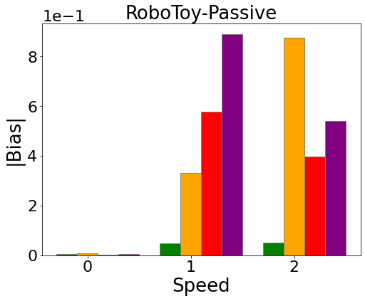
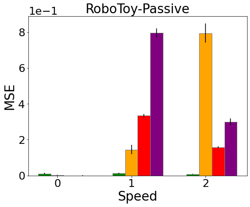
Figure 9: Comparison of different algorithms for predicting the future performance of evaluation policy $\pi$ on domains that exhibit passive non-stationarity. On the x-axis is the speed, which corresponds to the rate of non-stationarity; higher speed indicates a faster rate of change and a speed of zero indicates a stationary domain. (TOP) On the y-axis is the absolute bias in the performance estimate. (Bottom) On the y-axis is the mean squared error (MSE) in the performance estimate. Lower is better for all of these plots. For each domain, for each speed, for each algorithm, 30 trials were executed. Discussion of these plots can be found in Section E.4.

E.5 Ablation Study

In this section we study the sensitivity to hyper-parameters for the proposed method OPEN and the baseline method Pro-WLS [Chandak et al., 2020b]. The hyper-parameter for OPEN corresponds to the number of past terms to condition on for auto-regression, as discussed in rem:p. The hyper-parameter for Pro-WLS corresponds to the order of Fourier bases required for parametric regression. In Figure 10 we present the results for how the performance of the methods vary for different choices of hyper-parameters.

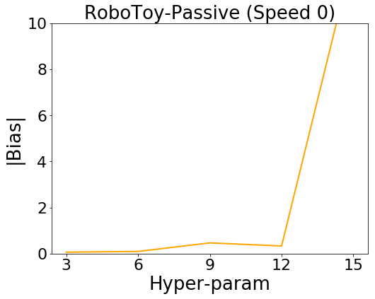
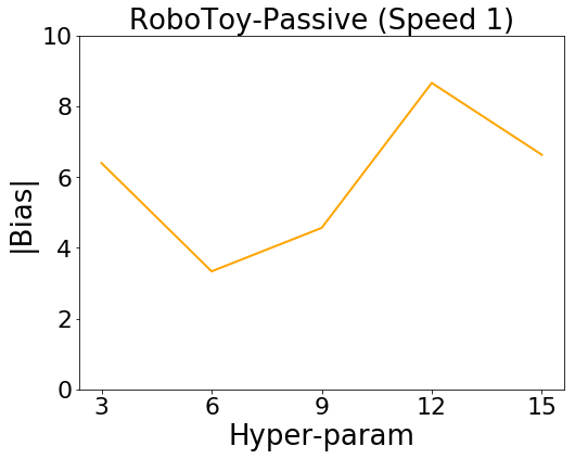
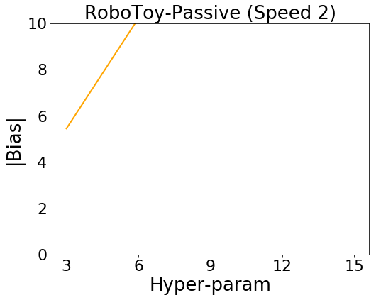
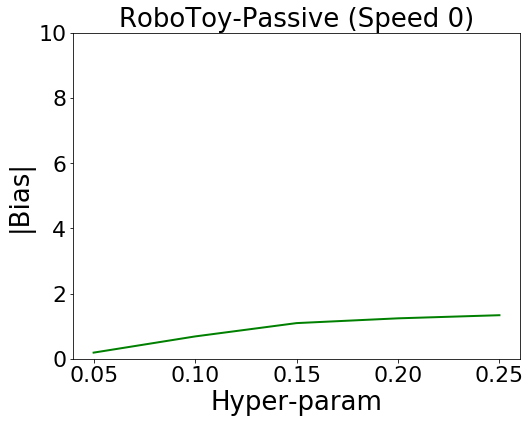
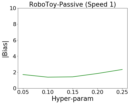
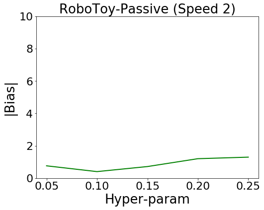
Figure 10: (Top) Absolute bias in prediction of Pro-WLS for different choices of its hyper-parameter. (Bottom) Absolute bias in prediction of OPEN for different choices of its hyper-parameter. For all the plots, lower value is better. Overall, we observe that OPEN being an auto-regressive method can extrapolate/forecast better and is thus more robust to hyper-parameters than Pro-WLS that uses Fourier bases for regression and is not as good for extrapolation.

References

- Abbott (2007) M. Abbott. Instrumental variables (iv) estimation: An introduction, 2007. http://qed.econ.queensu.ca/pub/faculty/abbott/econ481/481note09_f07.pdf.
- Achen (2000) C. H. Achen. Why lagged dependent variables can suppress the explanatory power of other independent variables. In annual meeting of the political methodology section of the American political science association, UCLA, volume 20, pages 7–2000, 2000.
- Agarwal et al. (2020) A. Agarwal, M. Henaff, S. Kakade, and W. Sun. Pc-pg: Policy cover directed exploration for provable policy gradient learning. Advances in Neural Information Processing Systems, 33:13399–13412, 2020.
- Alegre et al. (2021) L. N. Alegre, A. L. Bazzan, and B. C. da Silva. Minimum-delay adaptation in non-stationary reinforcement learning via online high-confidence change-point detection. arXiv preprint arXiv:2105.09452, 2021.
- Ammar et al. (2015) H. B. Ammar, R. Tutunov, and E. Eaton. Safe policy search for lifelong reinforcement learning with sublinear regret. In International Conference on Machine Learning, pages 2361–2369. PMLR, 2015.
- Basso and Engel (2009) E. W. Basso and P. M. Engel. Reinforcement learning in non-stationary continuous time and space scenarios. In Artificial Intelligence National Meeting, volume 7, pages 1–8. Citeseer, 2009.
- Bellemare et al. (2017) M. F. Bellemare, T. Masaki, and T. B. Pepinsky. Lagged explanatory variables and the estimation of causal effect. The Journal of Politics, 79(3):949–963, 2017.
- Bennett et al. (2019) A. Bennett, N. Kallus, and T. Schnabel. Deep generalized method of moments for instrumental variable analysis. arXiv preprint arXiv:1905.12495, 2019.
- Bennett et al. (2021) A. Bennett, N. Kallus, L. Li, and A. Mousavi. Off-policy evaluation in infinite-horizon reinforcement learning with latent confounders. In International Conference on Artificial Intelligence and Statistics, pages 1999–2007. PMLR, 2021.
- Besbes et al. (2014) O. Besbes, Y. Gur, and A. Zeevi. Stochastic multi-armed-bandit problem with non-stationary rewards. In Advances in Neural Information Processing Systems, pages 199–207, 2014.
- Bowling (2005) M. Bowling. Convergence and no-regret in multiagent learning. In Advances in Neural Information Processing Systems, pages 209–216, 2005.
- Boyan (1999) J. A. Boyan. Least-squares temporal difference learning. In ICML, pages 49–56, 1999.
- Buckman et al. (2020) J. Buckman, C. Gelada, and M. G. Bellemare. The importance of pessimism in fixed-dataset policy optimization. arXiv preprint arXiv:2009.06799, 2020.
- Cameron (2019) A. C. Cameron. Instrument variables, 2019. http://cameron.econ.ucdavis.edu/e240a/ch04iv.pdf.
- Cetin and Celiktutan (2021) E. Cetin and O. Celiktutan. Learning pessimism for robust and efficient off-policy reinforcement learning. arXiv preprint arXiv:2110.03375, 2021.
- Chandak et al. (2020a) Y. Chandak, S. M. Jordan, G. Theocharous, M. White, and P. S. Thomas. Towards safe policy improvement for non-stationary mdps. Neural Information Processing Systems, 2020a.
- Chandak et al. (2020b) Y. Chandak, G. Theocharous, S. Shankar, S. Mahadevan, M. White, and P. S. Thomas. Optimizing for the future in non-stationary mdps. International Conference on Machine Learning, 2020b.
- Chandak et al. (2021) Y. Chandak, S. Niekum, B. da Silva, E. Learned-Miller, E. Brunskill, and P. S. Thomas. Universal off-policy evaluation. Advances in Neural Information Processing Systems, 34, 2021.
- Chandra (1991) T. K. Chandra. Extensions of rajchman’s strong law of large numbers. Sankhyā: The Indian Journal of Statistics, Series A, pages 118–121, 1991.
- Choi et al. (2000) S. P. Choi, D.-Y. Yeung, and N. L. Zhang. An environment model for nonstationary reinforcement learning. In Advances in Neural Information Processing Systems, pages 987–993, 2000.
- Cinelli et al. (2021) M. Cinelli, G. D. F. Morales, A. Galeazzi, W. Quattrociocchi, and M. Starnini. The echo chamber effect on social media. Proceedings of the National Academy of Sciences, 118(9), 2021.
- Conitzer and Sandholm (2007) V. Conitzer and T. Sandholm. Awesome: A general multiagent learning algorithm that converges in self-play and learns a best response against stationary opponents. Machine Learning, 67(1-2):23–43, 2007.
- Cox and Miller (2017) D. R. Cox and H. D. Miller. The theory of stochastic processes. Routledge, 2017.
- Da Silva et al. (2006) B. C. Da Silva, E. W. Basso, A. L. Bazzan, and P. M. Engel. Dealing with non-stationary environments using context detection. In Proceedings of the 23rd international conference on Machine learning, pages 217–224, 2006.
- Dai et al. (2020) B. Dai, O. Nachum, Y. Chow, L. Li, C. Szepesvári, and D. Schuurmans. Coindice: Off-policy confidence interval estimation. arXiv preprint arXiv:2010.11652, 2020.
- Doshi-Velez and Konidaris (2016) F. Doshi-Velez and G. Konidaris. Hidden parameter markov decision processes: A semiparametric regression approach for discovering latent task parametrizations. In IJCAI: proceedings of the conference, volume 2016, page 1432. NIH Public Access, 2016.
- Dulac-Arnold et al. (2019) G. Dulac-Arnold, D. Mankowitz, and T. Hester. Challenges of real-world reinforcement learning. arXiv preprint arXiv:1904.12901, 2019.
- Espeholt et al. (2018) L. Espeholt, H. Soyer, R. Munos, K. Simonyan, V. Mnih, T. Ward, Y. Doron, V. Firoiu, T. Harley, I. Dunning, et al. Impala: Scalable distributed deep-rl with importance weighted actor-learner architectures. In International conference on machine learning, pages 1407–1416. PMLR, 2018.
- Feng et al. (2021) Y. Feng, Z. Tang, na zhang, and qiang liu. Non-asymptotic confidence intervals of off-policy evaluation: Primal and dual bounds. In International Conference on Learning Representations, 2021. URL https://openreview.net/forum?id=dKg5D1Z1Lm.
- Foerster et al. (2018) J. Foerster, R. Y. Chen, M. Al-Shedivat, S. Whiteson, P. Abbeel, and I. Mordatch. Learning with opponent-learning awareness. In Proceedings of the 17th International Conference on Autonomous Agents and MultiAgent Systems, pages 122–130. International Foundation for Autonomous Agents and Multiagent Systems, 2018.
- Foster et al. (2016) D. J. Foster, Z. Li, T. Lykouris, K. Sridharan, and E. Tardos. Learning in games: Robustness of fast convergence. In Advances in Neural Information Processing Systems, pages 4734–4742, 2016.
- Gemp and Mahadevan (2017) I. Gemp and S. Mahadevan. Online monotone games. arXiv preprint arXiv:1710.07328, 2017.
- Gillani et al. (2018) N. Gillani, A. Yuan, M. Saveski, S. Vosoughi, and D. Roy. Me, my echo chamber, and i: introspection on social media polarization. In Proceedings of the 2018 World Wide Web Conference, pages 823–831, 2018.
- Hamilton (1994) J. D. Hamilton. State-space models. Handbook of econometrics, 4:3039–3080, 1994.
- Hartford et al. (2017) J. Hartford, G. Lewis, K. Leyton-Brown, and M. Taddy. Deep iv: A flexible approach for counterfactual prediction. In International Conference on Machine Learning, pages 1414–1423. PMLR, 2017.
- Harutyunyan et al. (2016) A. Harutyunyan, M. G. Bellemare, T. Stepleton, and R. Munos. Q ( ) with off-policy corrections. In International Conference on Algorithmic Learning Theory, pages 305–320. Springer, 2016.
- Hennes et al. (2019) D. Hennes, D. Morrill, S. Omidshafiei, R. Munos, J. Perolat, M. Lanctot, A. Gruslys, J.-B. Lespiau, P. Parmas, E. Duenez-Guzman, et al. Neural replicator dynamics. arXiv preprint arXiv:1906.00190, 2019.
- Hochreiter and Schmidhuber (1997) S. Hochreiter and J. Schmidhuber. Long short-term memory. Neural computation, 9(8):1735–1780, 1997.
- Jagerman et al. (2019) R. Jagerman, I. Markov, and M. de Rijke. When people change their mind: Off-policy evaluation in non-stationary recommendation environments. In Proceedings of the Twelfth ACM International Conference on Web Search and Data Mining, Melbourne, VIC, Australia, February 11-15, 2019, 2019.
- Jaques et al. (2019) N. Jaques, A. Lazaridou, E. Hughes, C. Gulcehre, P. Ortega, D. Strouse, J. Z. Leibo, and N. De Freitas. Social influence as intrinsic motivation for multi-agent deep reinforcement learning. In International Conference on Machine Learning, pages 3040–3049. PMLR, 2019.
- Jiang and Huang (2020) N. Jiang and J. Huang. Minimax confidence interval for off-policy evaluation and policy optimization. arXiv preprint arXiv:2002.02081, 2020.
- Jiang and Li (2015) N. Jiang and L. Li. Doubly robust off-policy value evaluation for reinforcement learning. arXiv preprint arXiv:1511.03722, 2015.
- Khetarpal et al. (2020) K. Khetarpal, M. Riemer, I. Rish, and D. Precup. Towards continual reinforcement learning: A review and perspectives. arXiv preprint arXiv:2012.13490, 2020.
- Levine et al. (2017) N. Levine, K. Crammer, and S. Mannor. Rotting bandits. In Advances in Neural Information Processing Systems, pages 3074–3083, 2017.
- Li and de Rijke (2019) C. Li and M. de Rijke. Cascading non-stationary bandits: Online learning to rank in the non-stationary cascade model. arXiv preprint arXiv:1905.12370, 2019.
- Liotet et al. (2021) P. Liotet, F. Vidaich, A. M. Metelli, and M. Restelli. Lifelong hyper-policy optimization with multiple importance sampling regularization. arXiv preprint arXiv:2112.06625, 2021.
- Liu et al. (2018) Q. Liu, L. Li, Z. Tang, and D. Zhou. Breaking the curse of horizon: Infinite-horizon off-policy estimation. In Advances in Neural Information Processing Systems, pages 5356–5366, 2018.
- Liu et al. (2020) R. Liu, Z. Shang, and G. Cheng. On deep instrumental variables estimate. arXiv preprint arXiv:2004.14954, 2020.
- Mahmood et al. (2014) A. R. Mahmood, H. Van Hasselt, and R. S. Sutton. Weighted importance sampling for off-policy learning with linear function approximation. In NIPS, pages 3014–3022, 2014.
- Mahmood et al. (2015) A. R. Mahmood, H. Yu, M. White, and R. S. Sutton. Emphatic temporal-difference learning. arXiv preprint arXiv:1507.01569, 2015.
- Man et al. (2014) C. D. Man, F. Micheletto, D. Lv, M. Breton, B. Kovatchev, and C. Cobelli. The UVA/PADOVA type 1 diabetes simulator: New features. Journal of Diabetes Science and Technology, 8(1):26–34, 2014.
- Mealing and Shapiro (2013) R. Mealing and J. L. Shapiro. Opponent modelling by sequence prediction and lookahead in two-player games. In International Conference on Artificial Intelligence and Soft Computing, pages 385–396. Springer, 2013.
- Moore (1990) A. W. Moore. Efficient memory-based learning for robot control. 1990.
- Moulines (2008) E. Moulines. On upper-confidence bound policies for non-stationary bandit problems. arXiv preprint arXiv:0805.3415, 2008.
- Munos et al. (2016) R. Munos, T. Stepleton, A. Harutyunyan, and M. Bellemare. Safe and efficient off-policy reinforcement learning. Advances in neural information processing systems, 29, 2016.
- Nachum and Dai (2020) O. Nachum and B. Dai. Reinforcement learning via fenchel-rockafellar duality. arXiv preprint arXiv:2001.01866, 2020.
- Nachum et al. (2019) O. Nachum, Y. Chow, B. Dai, and L. Li. Dualdice: Behavior-agnostic estimation of discounted stationary distribution corrections. Advances in Neural Information Processing Systems, 32, 2019.
- Namkoong et al. (2020) H. Namkoong, R. Keramati, S. Yadlowsky, and E. Brunskill. Off-policy policy evaluation for sequential decisions under unobserved confounding. Advances in Neural Information Processing Systems, 33:18819–18831, 2020.
- Padakandla (2020) S. Padakandla. A survey of reinforcement learning algorithms for dynamically varying environments. arXiv preprint arXiv:2005.10619, 2020.
- Padakandla et al. (2019) S. Padakandla, P. K. J., and S. Bhatnagar. Reinforcement learning in non-stationary environments. CoRR, abs/1905.03970, 2019.
- Parker (2020) J. A. Parker. Endogenous regressors and instrumental variables, 2020. https://www.reed.edu/economics/parker/312/notes/Notes11.pdf.
- Pearl et al. (2000) J. Pearl et al. Models, reasoning and inference. Cambridge, UK: CambridgeUniversityPress, 19, 2000.
- Poiani et al. (2021) R. Poiani, A. Tirinzoni, and M. Restelli. Meta-reinforcement learning by tracking task non-stationarity. arXiv preprint arXiv:2105.08834, 2021.
- Precup (2000) D. Precup. Eligibility traces for off-policy policy evaluation. Computer Science Department Faculty Publication Series, page 80, 2000.
- Puterman (1990) M. L. Puterman. Markov decision processes. Handbooks in operations research and management science, 2:331–434, 1990.
- Rachelson et al. (2009) E. Rachelson, P. Fabiani, and F. Garcia. Timdppoly: An improved method for solving time-dependent mdps. In 2009 21st IEEE International Conference on Tools with Artificial Intelligence, pages 796–799. IEEE, 2009.
- Rajchman (1932) A. Rajchman. Zaostrzone prawo wielkich liczb. Mathesis Polska, 6:145–161, 1932.
- Reed (2015) W. R. Reed. On the practice of lagging variables to avoid simultaneity. Oxford Bulletin of Economics and Statistics, 77(6):897–905, 2015.
- Robbins et al. (2020) M. J. Robbins, P. R. Jenkins, N. D. Bastian, and B. J. Lunday. Approximate dynamic programming for the aeromedical evacuation dispatching problem: Value function approximation utilizing multiple level aggregation. Omega, 91:102020, 2020.
- Russac et al. (2019) Y. Russac, C. Vernade, and O. Cappé. Weighted linear bandits for non-stationary environments. Advances in Neural Information Processing Systems, 32, 2019.
- Seznec et al. (2018) J. Seznec, A. Locatelli, A. Carpentier, A. Lazaric, and M. Valko. Rotting bandits are no harder than stochastic ones. arXiv preprint arXiv:1811.11043, 2018.
- Shi et al. (2021) C. Shi, M. Uehara, and N. Jiang. A minimax learning approach to off-policy evaluation in partially observable markov decision processes. arXiv preprint arXiv:2111.06784, 2021.
- Singh et al. (2000) S. Singh, M. Kearns, and Y. Mansour. Nash convergence of gradient dynamics in general-sum games. In Proceedings of the Sixteenth conference on Uncertainty in artificial intelligence, pages 541–548. Morgan Kaufmann Publishers Inc., 2000.
- Sutton and Barto (2018) R. S. Sutton and A. G. Barto. Reinforcement learning: An introduction. MIT Press, Cambridge, MA, 2 edition, 2018.
- Sutton et al. (2008) R. S. Sutton, H. Maei, and C. Szepesvári. A convergent temporal-difference algorithm for off-policy learning with linear function approximation. Advances in neural information processing systems, 21, 2008.
- Sutton et al. (2009) R. S. Sutton, H. R. Maei, D. Precup, S. Bhatnagar, D. Silver, C. Szepesvári, and E. Wiewiora. Fast gradient-descent methods for temporal-difference learning with linear function approximation. In Proceedings of the 26th annual international conference on machine learning, pages 993–1000, 2009.
- Taiga et al. (2021) A. A. Taiga, W. Fedus, M. C. Machado, A. Courville, and M. G. Bellemare. On bonus-based exploration methods in the arcade learning environment. arXiv preprint arXiv:2109.11052, 2021.
- Tennenholtz et al. (2020) G. Tennenholtz, U. Shalit, and S. Mannor. Off-policy evaluation in partially observable environments. In Proceedings of the AAAI Conference on Artificial Intelligence, volume 34, pages 10276–10283, 2020.
- Theocharous et al. (2020) G. Theocharous, Y. Chandak, P. S. Thomas, and F. de Nijs. Reinforcement learning for strategic recommendations. arXiv preprint arXiv:2009.07346, 2020.
- Thomas and Brunskill (2016) P. Thomas and E. Brunskill. Data-efficient off-policy policy evaluation for reinforcement learning. In International Conference on Machine Learning, pages 2139–2148, 2016.
- Thomas et al. (2015) P. Thomas, G. Theocharous, and M. Ghavamzadeh. High-confidence off-policy evaluation. In Proceedings of the AAAI Conference on Artificial Intelligence, volume 29, 2015.
- Thomas (2015) P. S. Thomas. Safe reinforcement learning. PhD thesis, University of Massachusetts Libraries, 2015.
- Thomas et al. (2017) P. S. Thomas, G. Theocharous, M. Ghavamzadeh, I. Durugkar, and E. Brunskill. Predictive off-policy policy evaluation for nonstationary decision problems, with applications to digital marketing. In AAAI, pages 4740–4745, 2017.
- Thomas et al. (2019) P. S. Thomas, B. C. da Silva, A. G. Barto, S. Giguere, Y. Brun, and E. Brunskill. Preventing undesirable behavior of intelligent machines. Science, 366(6468):999–1004, 2019.
- Uehara et al. (2020) M. Uehara, J. Huang, and N. Jiang. Minimax weight and q-function learning for off-policy evaluation. In International Conference on Machine Learning, pages 9659–9668. PMLR, 2020.
- Vernade et al. (2020) C. Vernade, A. Gyorgy, and T. Mann. Non-stationary delayed bandits with intermediate observations. In International Conference on Machine Learning, pages 9722–9732. PMLR, 2020.
- Wang et al. (2019a) L. Wang, H. Zhou, B. Li, L. R. Varshney, and Z. Zhao. Be aware of non-stationarity: Nearly optimal algorithms for piecewise-stationary cascading bandits. arXiv preprint arXiv:1909.05886, 2019a.
- Wang et al. (2007) T. Wang, M. Bowling, and D. Schuurmans. Dual representations for dynamic programming and reinforcement learning. In 2007 IEEE International Symposium on Approximate Dynamic Programming and Reinforcement Learning, pages 44–51. IEEE, 2007.
- Wang et al. (2019b) T. Wang, J. Wang, Y. Wu, and C. Zhang. Influence-based multi-agent exploration. arXiv preprint arXiv:1910.05512, 2019b.
- Wang et al. (2021) W. Z. Wang, A. Shih, A. Xie, and D. Sadigh. Influencing towards stable multi-agent interactions. arXiv preprint arXiv:2110.08229, 2021.
- Wang and Bellemare (2019) Y. Wang and M. F. Bellemare. Lagged variables as instruments, 2019.
- Wilkins (2018) A. S. Wilkins. To lag or not to lag?: Re-evaluating the use of lagged dependent variables in regression analysis. Political Science Research and Methods, 6(2):393–411, 2018.
- Xie et al. (2020a) A. Xie, J. Harrison, and C. Finn. Deep reinforcement learning amidst lifelong non-stationarity. arXiv preprint arXiv:2006.10701, 2020a.
- Xie et al. (2020b) A. Xie, D. P. Losey, R. Tolsma, C. Finn, and D. Sadigh. Learning latent representations to influence multi-agent interaction. arXiv preprint arXiv:2011.06619, 2020b.
- Xie (2019) J. Xie. Simglucose v0.2.1 (2018), 2019. URL https://github.com/jxx123/simglucose.
- Xie et al. (2019) T. Xie, Y. Ma, and Y.-X. Wang. Towards optimal off-policy evaluation for reinforcement learning with marginalized importance sampling. arXiv preprint arXiv:1906.03393, 2019.
- Xu et al. (2020) L. Xu, Y. Chen, S. Srinivasan, N. de Freitas, A. Doucet, and A. Gretton. Learning deep features in instrumental variable regression. arXiv preprint arXiv:2010.07154, 2020.
- Yang et al. (2020) M. Yang, O. Nachum, B. Dai, L. Li, and D. Schuurmans. Off-policy evaluation via the regularized lagrangian. Advances in Neural Information Processing Systems, 33:6551–6561, 2020.
- Yuan et al. (2021) C. Yuan, Y. Chandak, S. Giguere, P. S. Thomas, and S. Niekum. Sope: Spectrum of off-policy estimators. Advances in Neural Information Processing Systems, 34:18958–18969, 2021.
- Zhang and Lesser (2010) C. Zhang and V. Lesser. Multi-agent learning with policy prediction. In Twenty-fourth AAAI conference on artificial intelligence, 2010.
- Zhou et al. (2020) H. Zhou, J. Chen, L. R. Varshney, and A. Jagmohan. Nonstationary reinforcement learning with linear function approximation. arXiv preprint arXiv:2010.04244, 2020.