Probing gamma-ray bursts observed at very high energies through their afterglow

Abstract

A growing number of gamma-ray burst (GRB) afterglows is observed at very-high energies (VHE, $\gtrsim 100$ GeV). Yet, our understanding of the mechanism powering the VHE emission remains baffling. We make use of multi-wavelength observations of the afterglow of GRB 180720B, GRB 190114C, and GRB 221009A to investigate whether the bursts exhibiting VHE emission share common features. We assume the standard afterglow model and microphysical parameters consistent with a synchrotron self-Compton (SSC) scenario for the VHE radiation. By requiring that the blastwave should be transparent to $\gamma$–$\gamma$ pair production at the time of observation of the VHE photons and relying on typical prompt emission efficiencies and data in the radio, optical and X-ray bands, we infer for those bursts that the initial energy of the blastwave is $\tilde{E}_{k,\rm{iso}}\gtrsim\mathcal{O}(10^{54})$ erg and the circumburst density is $n_{0}\lesssim\mathcal{O}(10^{-1})$ cm^-3 for a constant circumburst profile [or $A_{\star}\lesssim\mathcal{O}(10^{-1})$ cm^-1 for a wind scenario]. Our findings thus suggest that these VHE bursts might be hosted in low-density environments, if the SSC radiation is responsible for the VHE emission. While these trends are based on a small number of bursts, the Cherenkov Telescope Array has the potential to provide crucial insight in this context by detecting a larger sample of VHE GRBs. In addition, due to the very poor statistics, the non-observation of high-energy neutrinos cannot constrain the properties of these bursts efficiently, unless additional VHE GRBs should be detected at distances closer than $15$ Mpc when IceCube-Gen2 radio will be operational.

1 Introduction

Gamma-ray bursts (GRBs) are among the most powerful explosions in our Universe (Klebesadel et al., 1973; Kumar & Zhang, 2014; Piran, 2004). They exhibit a non-thermal spectrum with typical peak energies in the keV–MeV range (Poolakkil et al., 2021; von Kienlin et al., 2020; Ford et al., 1995). We focus on long-duration GRBs, which release an isotropic energy in gamma-rays of about $10^{49}$–$10^{55}$ ergs within a few $\mathcal{O}(10)$ s (Kumar & Zhang, 2014; Atteia et al., 2017). The pulse of gamma-rays released during the prompt phase is followed by a delayed, long-lasting emission: the afterglow. Being detected from the radio to the X-ray bands, the afterglow makes GRBs electromagnetically accessible across all wavebands (e.g., Meszaros & Rees, 1997).

Afterglow detections at high energy (HE, $\gtrsim 1$ GeV) have been reported for more than a decade, e.g. by the Large Area Telescope (LAT) onboard of the Fermi satellite (Ajello et al., 2019). In the past few years, such observations have been complemented by the detection of very high energy (VHE, $\gtrsim 100$ GeV) emission from an increasing number of GRBs, with photons with $\mathcal{O}(\rm{TeV})$ energy being detected several hours after the burst trigger (Abdalla et al., 2019, 2021; Acciari et al., 2019b, a; Suda et al., 2021; Fukami et al., 2021). Among these puzzling bursts, the recently discovered GRB 221009A represents an extraordinary event, being located close-by ($z\simeq 0.15$), very bright in gamma-rays ($\tilde{E}_{\gamma,\rm{iso}}\gtrsim 3\times 10^{54}$ ergs) , and detected with photons up to $\mathcal{O}(10)$ TeV by the Large High Altitude Air Shower Observatory (LHAASO) (Huang et al., 2022).

The VHE emission associated with the GRB afterglow was theoretically predicted (Meszaros et al., 1994; Dermer et al., 2000; Meszaros, 2002; Piran, 2004; Kumar & Zhang, 2014), and then observed thanks to ground-based Cherenkov telescopes, such as the High Energy Stereoscopic System (H.E.S.S.) and the Major Atmospheric Gamma Imaging Cherenkov (MAGIC). The detection rate of GRB photons with energies $\gtrsim\mathcal{O}(\rm{TeV})$ is expected to further improve with LHAASO (Huang et al., 2022) and the upcoming Cherenkov Telescope Array (CTA) (Knödlseder, 2020); hence, it is timely to investigate under which conditions VHE emission should be expected.

Up to HE, the multi-wavelength emission of the GRB afterglow is broadly considered to be generated by the synchrotron radiation produced by the electrons accelerated at the external shock as the latter expands in the circumburst medium (CBM) (Meszaros & Rees, 1997; Waxman, 1997b, a; Katz & Piran, 1997; Sari et al., 1998). Yet, this standard afterglow picture cannot accommodate the production of TeV photons, unless electrons are accelerated above the synchrotron cut-off energy—see, e.g., Abdalla et al. (2021).

A possibility proposed to explain the VHE emission is the synchrotron self-Compton (SSC) scenario, according to which synchrotron photons inverse-Compton scatter the electrons that produced them (Ghisellini & Celotti, 1999; Chiang & Dermer, 1999; Dermer, 2002; Sari & Esin, 2001; Nakar et al., 2009; Liu et al., 2013; Derishev & Piran, 2021; Fraija et al., 2019b; Asano et al., 2020; Khangulyan et al., 2023). Alternatively, the acceleration of baryons together with electrons at the external shock can be considered. In this case, the mechanism responsible for the VHE emission may be proton synchrotron radiation or the decay of secondaries produced in photo-pion and photo-pair processes (e.g., Bottcher & Dermer, 1998; Asano et al., 2009; Razzaque et al., 2010; Gagliardini et al., 2022; Isravel et al., 2022). Photohadronic processes have also been invoked for modeling the VHE emission (e.g., Sahu & López Fortín, 2020; Sahu et al., 2022).

While the number of GRBs detected in the VHE regime in the afterglow increases, our understanding of the physics underlying these bursts remains superficial. Do GRBs with VHE emission share common properties? Can we use VHE observations to infer properties of the CBM? In this paper, we intend to infer the characteristic features of GRBs exhibiting VHE emission and explore whether these bursts occur in environments with similar properties, possibly different from the ones expected from typical Wolf-Rayet stars observed in our Galaxy (e.g. Schulze et al., 2011; Crowther, 2007).

This paper is organized as follows. Section 2 presents an outline of the properties of the bursts detected in the VHE regime. In Sec. 3, we review the afterglow model, the blaswave dynamics and the related synchrotron radiation. We present constraints on the GRB energetics and the initial Lorentz factor in Sec. 4, while constraints on the non-observation of neutrinos from these bursts are presented in Sec. 5. A discussion on our findings is reported in Sec. 6, before concluding in Sec. 7. The modeling of the photon energy distribution is summarized in Appendix A, while the physics of hadronic interactions is outlined in Appendix B. Appendix C provides additional insight on the properties of the CBM for our VHE GRB sample in comparison with GRBs without VHE emission.

2 Sample of gamma-ray bursts observed at very high energies

The GRBs detected with VHE emission can be broadly grouped in two classes based on the isotropic energy emitted in gamma-rays during the prompt phase: GRBs with intermediate to low isotropic energy [$\tilde{E}_{\mathrm{\gamma,\rm{iso}}}\lesssim 10^{50}$ erg, i.e. GRB 201015A (Suda et al., 2021) and GRB 190829A (Abdalla et al., 2021)] and energetic events with isotropic energy larger than typically observed ($\tilde{E}_{\mathrm{\gamma,\rm{iso}}}\gtrsim 10^{53}$ erg). We limit our analysis to the latter group.

The class of bursts detected in the VHE regime and with large $\tilde{E}_{\gamma,\rm{iso}}$ is populated by:

• GRB 180720B detected with $\tilde{E}_{\gamma,\rm{iso}}\simeq 6\times 10^{53}$ erg (Frederiks et al., 2018). The H.E.S.S. Collaboration reported the observation of photons with energy between $0.11$ TeV and $0.44$ TeV at about $\sim 10$ hours after the trigger (Abdalla et al., 2019).

• GRB 190114C, whose isotropic energy is estimated to be $\tilde{E}_{\gamma,\rm{iso}}\simeq 2.5\times 10^{53}$ (Hamburg et al., 2019). MAGIC observed $0.3$–$1$ TeV photons (Acciari et al., 2019b, a) from this burst, starting approximately one minute after its trigger. From Fig. 3 of Acciari et al. (2019a), we infer that a large number of photons of energy up to $1$ TeV is still observed at late times, around $520$ s, when the emission can be associated with the afterglow.

• GRB 221009A observed with isotropic energy $\tilde{E}_{\gamma,\rm{iso}}\gtrsim 3\times 10^{54}$ erg (de Ugarte Postigo et al., 2022; Frederiks et al., 2022; Kann & Agui Fernandez, 2022). This is an interesting burst with photons with energy up to $18$ TeV reported by LHAASO within $2000$ s post GBM trigger (Huang et al., 2022; Xia et al., 2022). The distribution in energy and time of the VHE photons is not yet available,while upper limits on the VHE flux at very late times have been published by H.E.S.S. (Aharonian et al., 2023). On the contrary, the photon with energy $\simeq 0.4$ TeV detected $0.4$ days after the trigger of the burst by Fermi-LAT can be safely associated with the afterglow emission (Xia et al., 2022).

Note that VHE emission has been observed from GRB 201216C as well, whose prompt isotropic energy is $\tilde{E}_{\gamma,\rm{iso}}\simeq 4.7\times 10^{53}$ erg (Frederiks et al., 2020). Since the published data is sparse to date (Fukami et al., 2021), we do not consider this GRB in our analysis. The properties of the sample of GRBs that we consider throughout this paper are summarized in Table 1.

Table 1: Properties of the sample of VHE GRBs considered in this work. For each GRB we list the redshift ($z$), the inferred emitted isotropic energy of the prompt phase in the source frame ($\tilde{E}_{\mathrm{\gamma,{iso}}}$), the duration of the prompt emission ($T_{90}$), the time of detection of the VHE photon ($T_{\gamma,\rm{VHE}}$), the electron spectral index ($k_{e}$) and the CBM type (wind or ISM). The following references are quoted in the table: [1] Roberts & Meegan (2018), [2] Frederiks et al. (2018), [3] Abdalla et al. (2019), [4] Acciari et al. (2019b), [5] Acciari et al. (2019a), [6] Gropp et al. (2019), [7] Acciari et al. (2019b), [8] Misra et al. (2019), [9] Huang et al. (2022), [10] Xia et al. (2022), [11] Lesage et al. (2022), [12] Belkin et al. (2022).

Event	Redshift	$\tilde{E}_{\mathrm{\gamma,iso}}$ [erg]	$T_{90}$ [s]	$T_{\rm{VHE}}$ [days]	$k_{e}$	CBM	References
GRB 180720B	0.653	$6\times 10^{53}$	$49$	$0.5$	$2.4$	ISM	[1, 2, 3]
GRB 190114C	0.4245	$2.5\times 10^{53}$	$25$	$6\times 10^{-3}$	$2.2$–$2.45$	ISM	[4, 5, 6, 7, 8]
GRB 221009A	0.151	$3\times 10^{54}$	$300$	$0.3$	$2.5$	Wind	[9, 10, 11, 12]

3 Afterglow model

In this section, we review the dynamics of the GRB blastwave as it propagates in the CBM. We also introduce the synchrotron spectrum invoked to model the standard afterglow emission.

3.1 Blastwave dynamics

Throughout the prompt phase, the Lorentz factor of GRB outflows is $\Gamma\gg 100$ (Gehrels et al., 2009). During the afterglow, $\Gamma^{-1}\lesssim\theta_{j}$, being $\theta_{j}$ the jet half-opening angle. Therefore, it is safe to model the afterglow radiation through isotropic equivalent quantities (Kumar & Zhang, 2014). We introduce the kinetic isotropic energy of the blastwave, $\tilde{E}_{k,\rm{iso}}=\tilde{E}_{\rm{iso}}-\tilde{E}_{\gamma,\rm{iso}}$, corresponding to the energy left in the outflow after the isotropic energy $\tilde{E}_{\gamma,\rm{iso}}$ has been released in gamma-rays during the prompt emission.

In the standard picture, the onset of the afterglow coincides with the beginning of the blastwave deceleration, occurring as the mass swept-up from the CBM becomes comparable to the initial mass of the outflow (e.g., Zhang, 2018, and references therein). The CBM is assumed to have particle density profiles scaling as $n\propto R^{-k}$, where $R$ is the distance from the central engine. Two asymptotic scenarios are usually considered in the literature (Schulze et al., 2011): $k=0$, corresponding to a constant density interstellar medium (hereafter named ISM), and $k=2$, corresponding to a wind-like CBM (hereafter dubbed wind).

As the blastwave expands, it interacts with the cold CBM. Two shocks form: the forward shock, which propagates in the cold CBM, and the reverse shock, propagating in the relativistic jet, in mass coordinates. We focus on the self-similar phase, starting when the reverse shock has crossed the ejecta and the electromagnetic emission is mainly due to the forward shock. In this phase, the blastwave dynamics is well described by the Blandford-McKee (BM) solution (Blandford & McKee, 1976).

The deceleration time of the blastwave depends on the particle density profile of the CBM. Assuming that the outflow is launched with initial Lorentz factor $\Gamma_{0}$ in the ISM scenario (Blandford & McKee, 1976; Zhang, 2018):

$$T_{\rm{dec,ISM}}=\left[\frac{3\tilde{E}_{k,\rm{iso}}(1+z)^{3}}{64\pi n_{0}m_{p}c^{5}\Gamma_{0}^{8}}\right]^{1/3}\ ,$$ (1)

where $n=n_{0}$ is the ISM density, $z$ is the redshift of the source, $c$ is the speed of light, and $m_{p}$ is the proton mass. As for the wind scenario, the number density of the CBM is parametrized as $n=AR^{-2}$. Here, $A=\dot{M}_{w}/(4\pi v_{w}m_{p})=3.02\times 10^{35}A_{\star}$ cm^-1, where $A_{\star}=\dot{M}_{-5}/v_{8}$ is given for the typical mass loss rate $\dot{M}_{-5}=\dot{M}/(10^{-5}M_{\odot}\;\rm{yr}^{-1})$ and wind velocity $v_{8}=v_{w}/(10^{8}\;\rm{cm}\;\;\rm{s}^{-1})$ of Wolf-Rayet stars (Chevalier & Li, 1999; Razzaque, 2013). According to this (Chevalier & Li, 2000):

$$T_{\rm{dec,wind}}=\frac{\tilde{E}_{k,\rm{iso}}(1+z)}{16\pi Am_{p}c^{3}\Gamma_{0}^{4}}\ .$$ (2)

After the deceleration starts, the Lorentz factor of the blastwave decreases with time (Blandford & McKee, 1976; Sari et al., 1998; Chevalier & Li, 2000):

$$\Gamma_{\rm{ISM}}=\Gamma_{0}\left(\frac{T_{\rm{dec,ISM}}}{4t}\right)^{3/8}\ ,$$ (3)

$$\Gamma_{\rm{wind}}=\Gamma_{0}\left(\frac{T_{\rm{dec,wind}}}{4t}\right)^{1/4}\ ,$$ (4)

for the ISM and wind scenarios, respectively.

Finally, the radius of the blastwave evolves as (Razzaque, 2013):

$$R=\frac{\zeta\Gamma^{2}tc}{(1+z)}\ ,$$ (5)

where $\Gamma$ decreases with time according to Eqs. 3 or 4, and we recall that the time $t$ is measured in the observer frame. The parameter $\zeta$ depends on the hydrodynamics of the blastwave. It is usually assumed to be constant, but its value is very uncertain (e.g., Sari et al., 1998; Waxman, 1997c; Dai & Lu, 1998; Derishev & Piran, 2021; Razzaque, 2013); throughout this work, we adopt $\zeta=8$ (Razzaque, 2013).

We assume the uniform shell approximation of the BM solution. This is a fair assumption, since we are not interested in the hydrodynamics of the blastwave. Furthermore, the particle density of the BM shell quickly drops outside the region of width $\propto R/\Gamma^{2}$ behind the forward shock. Hence, particle emission from outside this region is negligible.

3.2 Synchrotron spectrum

As the fireball expands in the cold CBM, the forward shock at its interface converts the kinetic energy of the blastwave into internal energy, whose density is given by (Blandford & McKee, 1976)

$$u^{\prime}=4m_{p}c^{2}n\Gamma\left(\Gamma-1\right)\ ,$$ (6)

where $n=n_{0}$ for the ISM scenario and $n=AR^{-2}$ in the wind scenario. Equation 6 directly follows from the shock-jump conditions at the forward shock.

A fraction $\varepsilon_{B}$ of the internal energy density in Eq. 6 is stored in the magnetic field, whose comoving strength is

$$B^{\prime}=\sqrt{32\pi m_{p}c^{2}n\varepsilon_{B}\Gamma(\Gamma-1)}\ .$$ (7)

The forward shock driven by the ejecta into the CBM is collisionless, meaning that it is mediated by collective plasma instabilities rather than collisions (Levinson & Nakar, 2020). Hence, it can accelerate particles through the Fermi mechanism (Waxman, 1995; Vietri, 1995; Waxman, 2000). In particular, we assume that electrons are accelerated to a power-law distribution $N(\gamma_{e})\propto\gamma_{e}^{-k_{e}}$, where $k_{e}$ is the electron spectral index. The resulting non-thermal population of accelerated electrons is assumed to carry a fraction $\varepsilon_{e}$ of the energy density (Eq. 6).

Three characteristic Lorentz factors define the distribution of shock-accelerated electrons: the minimum ($\gamma^{\prime}_{e,\rm{min}}$), the cooling ($\gamma^{\prime}_{e,\rm{cool}}$), and the maximum ($\gamma^{\prime}_{e,\max}$) ones. These are given by (Piran, 2004; Chevalier & Li, 2000; Panaitescu & Kumar, 2000):

$$\gamma^{\prime}_{e,\rm{min}} = \frac{\epsilon_{e}}{\xi_{e}}\frac{m_{p}}{m_{e}}{\frac{(k_{e}-2)}{(k_{e}-1)}(\Gamma-1)}\ ,$$ (8)

$$\gamma^{\prime}_{e,\rm{cool}} = \frac{6\pi m_{e}c}{\sigma_{T}B^{\prime 2}}\frac{(1+z)}{t\Gamma}\ ,$$ (9)

$$\gamma^{\prime}_{e,\rm{max}} = \biggl{(}\frac{6\pi e}{\sigma_{T}B^{\prime}\varphi}\biggr{)}^{1/2}\ ,$$ (10)

where $\sigma_{T}$ is the Thompson cross section, $\xi_{e}$ is the fraction of accelerated electrons, $e=\sqrt{\alpha\hbar c}$ is the electron charge, with $\alpha=1/137$ being the fine-structure constant, and $\hbar$ the reduced Planck constant. Finally, $\varphi$ is the number of gyroradii required to accelerate particles (Gao et al., 2012). The maximum Lorentz factor $\gamma^{\prime}_{e,\max}$ is obtained by equating the electron cooling time $t^{\prime}_{e,\rm{cool}}=6\pi m_{e}c/(\sigma_{T}\gamma^{\prime}_{e}B^{\prime 2})$ and the acceleration time $t^{\prime}_{\rm{acc}}=2\pi\gamma^{\prime}_{e}m_{e}c^{2}\varphi/(ecB^{\prime})$.

The synchrotron break frequencies in Eqs. 8–10 should take into account SSC losses of electrons, usually modeled through a correction factor depending on the Comptonization parameter $Y$ (for more details, see e.g. Sari & Esin, 2001). For all considered GRBs, observations show that the flux normalizations in the X-ray and VHE bands are comparable, hinting that synchrotron and SSC processes equally contribute to the cooling of electrons at the time of VHE emission. Since the $Y$ parameter decreases with time (Sari & Esin, 2001), and our analysis mainly considers epochs $t>T_{\rm{VHE}}$, we can safely neglect SSC corrections in Eqs. 8-10; see Sec. 4.1.

The characteristic Lorentz factors of electrons introduce three energy breaks in the observed spectrum of synchrotron photons, namely $E_{\gamma,\min}$, $E_{\gamma,\rm{cool}}$ and $E_{\gamma,\rm{max}}$, defined as (Sari et al., 1998):

$$E_{\gamma}\equiv h\nu_{\gamma}=\frac{3}{2}\frac{B^{\prime}}{B_{Q}}m_{e}c^{2}\gamma^{\prime\ 2}_{e}\frac{\Gamma}{(1+z)}\ ,$$ (11)

where $B_{Q}=4.41\times 10^{13}$ G.

The synchrotron self-absorption (SSA) Lorentz factor should be included for a complete treatment of synchrotron radiation. The corresponding break frequency is expected in the radio band (Zhang, 2018). However, detailed knowledge on the thermal electron distribution and on the structure of the emitting shell is needed to account for the SSA process (Warren et al., 2018). We neglect this characteristic Lorentz factor and corresponding break frequency and discuss how this choice affects our findings in Sec. 4.2.

Electrons can be in two distinct radiative regimes: the “fast cooling regime” (if $\nu_{\gamma,\rm{min}}>\nu_{\gamma,\rm{cool}}$) or the “slow cooling regime” (for $\nu_{\gamma,\rm{min}}<\nu_{\gamma,\rm{cool}}$). In the former case, all the electrons efficiently cool down via synchrotron to the cooling Lorentz factor $\gamma_{e,\rm{cool}}$. In the latter case, synchrotron cooling is inefficient and it takes place for electrons with $\gamma_{e}>\gamma_{e,\rm{cool}}$ only.

In the fast cooling regime, the synchrotron photon energy density [in units of GeV^-1 cm^-3] is (Sari et al., 1998):

$$n^{\prime\rm{sync}}_{\gamma}(E^{\prime}_{\gamma})=A^{\prime}_{\gamma}\left\{\begin{array}[]{@{}l@{}}\left(\frac{E^{\prime}_{\gamma}}{E^{\prime}_{\gamma,\rm{cool}}}\right)^{-\frac{2}{3}}\;\;\;\;\;\;\;\;\;\;\;\;\;\;\;\;\;E^{\prime}_{\gamma}<E^{\prime}_{\gamma,\rm{cool}}\\ \left(\frac{E^{\prime}_{\gamma}}{E^{\prime}_{\gamma,\rm{cool}}}\right)^{-\frac{3}{2}}\;\;\;\;\;\;\;\;\;\;\;\;\;\;\;\;\;E^{\prime}_{\gamma,\rm{cool}}\leq E^{\prime}_{\gamma}\leq E^{\prime}_{\gamma,\rm{min}}\\ \left(\frac{E^{\prime}_{\gamma,\rm{min}}}{E^{\prime}_{\gamma,\rm{cool}}}\right)^{-\frac{3}{2}}\left(\frac{E^{\prime}_{\gamma}}{E^{\prime}_{\gamma,\rm{min}}}\right)^{-\frac{k_{e}+2}{2}}E^{\prime}_{\gamma,\rm{min}}<E^{\prime}_{\gamma}\leq E^{\prime}_{\gamma,\rm{max}}\end{array}\right.\ .$$ (12)

On the other hand, in the slow cooling regime, the synchrotron photon energy density is:

$$n^{\prime\rm{sync}}_{\gamma}(E^{\prime}_{\gamma})=A^{\prime}_{\gamma}\left\{\begin{array}[]{@{}l@{}}\left(\frac{E^{\prime}_{\gamma}}{E^{\prime}_{\gamma,\min}}\right)^{-\frac{2}{3}}\;\;\;\;\;\;\;\;\;\;\;\;\;\;\;\;\;\;\;\;\;\;\;E^{\prime}_{\gamma}<E^{\prime}_{\gamma,\min}\\ \left(\frac{E^{\prime}_{\gamma}}{E^{\prime}_{\gamma,\min}}\right)^{-\frac{(k_{e}+1)}{2}}\;\;\;\;\;\;\;\;\;\;\;\;\;\;\;\;E^{\prime}_{\gamma,\min}\leq E^{\prime}_{\gamma}\leq E^{\prime}_{\gamma,\rm{cool}}\\ \left(\frac{E^{\prime}_{\gamma,\rm{cool}}}{E^{\prime}_{\gamma,\rm{min}}}\right)^{-\frac{k_{e}+1}{2}}\left(\frac{E^{\prime}_{\gamma}}{E^{\prime}_{\gamma,\rm{cool}}}\right)^{-\frac{k_{e}+2}{2}}E^{\prime}_{\gamma,\rm{cool}}<E^{\prime}_{\gamma}\leq E^{\prime}_{\gamma,\rm{max}}\end{array}\right.\ .$$ (13)

The normalization constant is given by (Sari et al., 1998; Dermer, 2002)

$$A^{\prime}_{\gamma}=\frac{L^{\prime}_{\gamma,\rm{max}}}{4\pi R^{2}c\;\min(E^{\prime}_{\gamma,\min},{E^{\prime}_{\gamma,\rm{cool}}})}\ ,$$ (14)

where $L^{\prime}_{\gamma,\rm{max}}=N_{e}P^{\prime}_{\max}(\gamma^{\prime}_{e})/E^{\prime}_{\gamma}$ is the comoving specific luminosity [in units of s^-1]. The total number of radiating electrons in the blastwave is $N_{e}=4\pi n_{0}\xi_{e}R^{3}/3$ in the ISM scenario, while it is given by $N_{e}=4\pi A\xi_{e}R$ in the wind scenario. Finally, the synchrotron power radiated by the electrons with Lorentz factor $\gamma^{\prime}_{e}=\min(\gamma^{\prime}_{e,\min},\gamma^{\prime}_{e,\rm{cool}})$ is $P^{\prime}_{\max}(\gamma^{\prime}_{e})=c\sigma_{T}B^{\prime\ 2}\gamma^{\prime\ 2}_{e}/{(6\pi)}$.

Given the photon energy density in Eqs. 12 and 13, the photon synchrotron spectrum observed at Earth is [in units of GeV cm^-2 s^-1 Hz^-1]:

$$\Phi^{\rm{sync}}_{\nu_{\gamma}}(E_{\gamma};z)=\frac{(1+z)^{2}}{4\pi d_{L}(z)^{2}}n^{\prime\ \rm{sync}}_{\gamma}\left(\frac{E_{\gamma}(1+z)}{\Gamma}\right)\frac{1}{\nu_{\gamma}}\frac{V^{\prime}_{\gamma}(1+z)}{t\Gamma}\ ,$$ (15)

where $V^{\prime}_{\gamma}=4\pi R^{3}/8\Gamma$ is the comoving emitting volume of the blastwave and $d_{L}(z)$ is the luminosity distance of the source at redshift $z$. We assume a flat $\Lambda$CDM cosmology with $H_{0}=67.4$ km s^-1 Mpc^-1, $\Omega_{M}=0.315$, and $\Omega_{\Lambda}=0.685$ (Zyla et al., 2020). The modeling of the (V)HE spectrum complementing the synchrotron one is described in Appendix A.

4 Constraints on the energetics and initial Lorentz factor

Table 2: Multi-wavelength fluxes used in our analysis for the bursts listed in Table 1. For each GRB, we list the considered observation time ($T_{\rm{obs}}$), as well as the correspondent radio flux ($F_{\nu,\rm{rad}}^{\rm{obs}}$), optical flux ($F_{\nu,\rm{opt}}^{\rm{obs}}$), and X-ray flux ($F_{\nu,\rm{X}}^{\rm{obs}}$); each at its corresponding frequency or bands, as specified in parenthesis. The following references are quoted in the table: [1] Sfaradi et al. (2018), [2] Fraija et al. (2019c), [3] Swift Burst Analyser (2022), [4] Misra et al. (2019), [5] Ren et al. (2022), [6] Farah et al. (2022); see also references therein for the extrapolated fluxes.

Burst	Tobs [days]	$F_{\nu,\rm{rad}}^{\rm{obs}}$ [Jy]	$F_{\nu,\rm{opt}}^{\rm{obs}}$ [Jy]	$F_{\nu,\rm{X}}^{\rm{obs}}$ [Jy]	References
GRB 180720B	$2$	$10^{-3}\;(15.5$ GHz)	$4\times 10^{-5}\;(R$-band)	$1.24\times 10^{-7}\;(10$ keV)	[1, 2, 3]
GRB 190114C	$1.424$	$1.930\times 10^{-3}\;(5.5$ GHz)	$3.9\times 10^{-5}\;(R-$band)	$5.98\times 10^{-8}\;(10$ keV)	[3, 4]
GRB 221009A	$2.3$	$9\times 10^{-3}\;(6$ GHz)	$2.016\times 10^{-3}\;(R-$ band)	$2.19\times 10^{-6}\;(10$ keV)	[3, 5, 6]

In this section, we present constraints on the blastwave energy and the surrounding CBM properties by exploiting the observed radio, optical and X-ray fluxes, and the opacity to $\gamma$–$\gamma$ pair production. By combining the observation of VHE photons with the duration of the prompt emission, we also infer upper and lower limits on the initial Lorentz factor $\Gamma_{0}$. We stress that we rely on the standard afterglow model outlined in Sec. 3. Hence, our constraints hold within this framework only.

Among the GRBs listed in Table 1, we select GRB 221009A and GRB 190114C to carry out our analysis. These GRBs are the closest ones and we consider them as representative of our sample in terms of energetics, see Sec. 2 and Table 1. Furthermore, they are good examples of the main models invoked to explain the VHE emission: SSC for GRB 221009A (Ren et al., 2022) and proton synchrotron for GRB 190114C (Isravel et al., 2022). The parameters listed in Table 1 are fixed in our analysis, while we consider $\tilde{E}_{k,\rm{iso}}$, $n$, $\varepsilon_{e}$, and $\varepsilon_{B}$ as free parameters in the model.

4.1 Multi-wavelength observations

As discussed in Sec. 3, the dynamics of the blastwave is independent of the initial Lorentz factor $\Gamma_{0}$, and it is completely determined by the isotropic kinetic energy $\tilde{E}_{k,\rm{iso}}$ and the CBM density $n$. Hence, by requiring that Eq. 15 matches the fluxes observed across different wavebands, we can constrain the allowed $\tilde{E}_{k,\rm{iso}}$ and $n$.

For GRB 221009A and GRB 190114C, the radio, optical and X-ray fluxes are extracted at the observation time $T_{\rm{obs}}$ where the data in the three wavebands are available. $T_{\rm{obs}}$ considered for each burst and the corresponding observed fluxes are listed in Table 2. Multi-wavelength light-curves and tables of data are provided in Misra et al. (2019) for GRB 190114C and in Ren et al. (2022) for GRB 221009A; see also references therein for observations with different instruments. The X-ray fluxes are obtained from the Swift Burst Analyser (2022).

We assume that the evolution of the emitting blast-wave is adiabatic, and that the micro-physical parameters of the emission are constant with time. Note that a different choice of $T_{\rm{obs}}$ would lead to the same order of magnitude estimation that we present here for $\tilde{E}_{k,\rm{iso}}$ and $n$. For convenience, we carry our analysis out at $T_{\rm{obs}}$ when radio, optical and X-ray data are simultaneously available for each GRB; see Table 2.

The left panels of Fig. 1 display the pairs of $(\tilde{E}_{k,\rm{iso}},n)$ for which Eq. 15 reproduces the fluxes observed in the radio, optical and X-ray bands, respectively, for GRB 190114C (top and middle panels) and GRB 221009A (bottom panel).

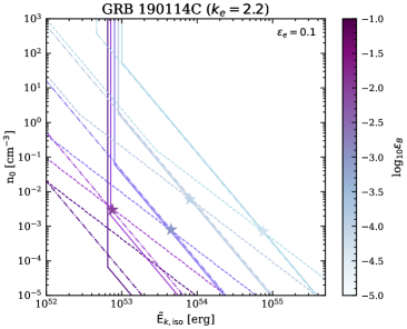
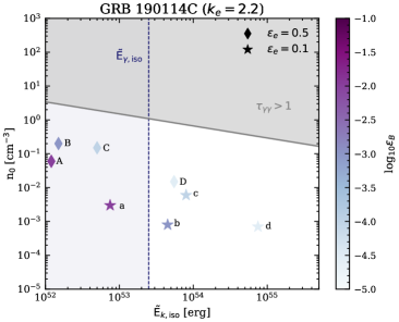
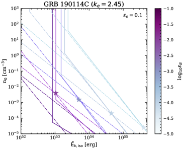
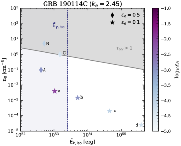
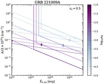
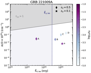
Figure 1: Isotropic kinetic energy $\tilde{E}_{k,\rm{iso}}$ and density $n_{0}\;[A/(3\times 10^{35})]$ compatible with the radio, optical and X-ray fluxes for GRB 190114C (top and middle panels) and GRB 221009A (bottom panels). Left panels: $(\tilde{E}_{k,\rm{iso}},n)$ pairs for which the computed synchrotron flux (Eq. 15) matches the observed one in the radio (dashed lines), optical (dotted-dashed lines) and X-ray (continuous lines), as listed in Table 2. For each burst, the line colors are defined by the value of $\varepsilon_{B}\in[10^{-5},10^{-1}]$ (see colorbar). For GRB 190114C, we fix $\varepsilon_{e}=0.1$ and $k_{e}=2.2$ in the top panels, while $k_{e}=2.45$ in the middle panels. For GRB 221009A, $\varepsilon_{e}=0.5$ and $k_{e}=2.6$; see main text for details. The intersection among the lines for each value of $\varepsilon_{B}$ is marked by a star ($\varepsilon_{e}=0.1$) or a diamond ($\varepsilon_{e}=0.5$). Results are shown for the value of $\varepsilon_{e}$ which guarantees solutions for $\varepsilon_{B}$ in the considered range. Right panels: Same as the left panels, but highlighting the pairs of $(\tilde{E}_{k,\rm{iso}},n)$ that simultaneously match radio, optical and X-ray data both for $\varepsilon_{e}=0.1$ (stars) and $\varepsilon_{e}=0.5$ (diamonds). The shadowed gray region is excluded from the transparency argument, i.e. $\tau_{\gamma\gamma}>1$ at $T_{\rm{VHE}}$ (Table 1). The dashed blue line marks the value of $\tilde{E}_{\gamma,\rm{iso}}$ for both bursts. Combining the transparency argument, the typical prompt emission efficiencies, and multi-wavelengths data, the preferred region of the parameter space for GRB 190114C [GRB 221009A] is the one with $2.5\times 10^{53}\lesssim\tilde{E}_{k,\rm{iso}}\lesssim 10^{55}$ erg [$3\times 10^{54}\lesssim\tilde{E}_{k,\rm{iso}}\lesssim 5\times 10^{55}$ erg] and $6\times 10^{-4}\lesssim n_{0}\lesssim 2\times 10^{-2}$ cm^-3 [$7\times 10^{-3}\lesssim A/(3\times 10^{35})\lesssim 10^{-1}$ cm^-1]. Note that the upper limit set for the kinetic energy is implied by the requirement that $\varepsilon_{B}$ cannot be too small in collisionless shocks. The letters mark the selected $(\tilde{E}_{k,\rm{iso}},n)$ pairs for which the corresponding initial Lorentz factor $\Gamma_{0}$ is reported in Table 3.

For GRB 190114C we calculate the theoretical synchrotron flux for two values of the electron spectral index: $k_{e}=2.2$ (top panels), which is obtained by inspecting the spectral energy distribution (Isravel et al., 2022), and $k_{e}=2.45$ (middle panels), which instead reproduces the slope of the lightcurve (Misra et al., 2019). For GRB 221009A, we only consider $k_{e}=2.6$ (Ren et al., 2022); see Table 1. In all cases, we fix $\xi_{e}=1$ throughout our analysis. The line colors in the left panels of Fig. 1 correspond to different values of $\varepsilon_{B}$, which we vary in the range $10^{-5}$–$10^{-1}$. For each $\varepsilon_{B}$ we select a value of $\varepsilon_{e}$ that allows for solutions, namely $\varepsilon_{e}=0.1$ (stars) and $\varepsilon_{e}=0.5$ (diamonds) for GRB 190114C and GRB 221009A, respectively. The intersection among the three lines in each of the left panels of Fig. 1, marked by a star (diamond), corresponds to the values of $\tilde{E}_{k,\rm{iso}}$ and $n$ which simultaneously reproduce the observed flux across the three wavebands for given pairs of ($\varepsilon_{e}$, $\varepsilon_{B}$).

The choice $\xi_{e}=1$ naturally excludes the proton synchrotron process for the modeling of the VHE emission, whereas it is consistent with the SSC scenario. The latter also requires $\varepsilon_{e}\gtrsim\varepsilon_{B}$, with typical parameters being $\varepsilon_{e}\simeq\mathcal{O}(10^{-1})$ and $\varepsilon_{B}\lesssim\mathcal{O}(10^{-2})$ (e.g., Sari & Esin, 2001); the relation between $\varepsilon_{e}$ and $\varepsilon_{B}$ is inverted in the proton synchroton scenario, that is to say $\varepsilon_{e}\ll\varepsilon_{B}$ (e.g. Razzaque et al., 2010; Isravel et al., 2022). Our assumptions are thus consistent with the SSC interpretation of the VHE emission. We discuss how this may affect our results in the following; see Sec. 4.2 and Sec. 6.

Note that we neglect any uncertainty on the observed fluxes and the microphysical parameters for simplicity, and the lines in the left panels of Fig. 1 are obtained by considering nominal values for the involved quantities. Furthermore, we rely on two approximations. First, we do not consider the exact hydrodynamics of the blastwave and adopt the uniform BM shell dynamics, as outlined in Sec. 3. Second, our results are sensitive to the constant $\zeta$ appearing in the definition of the blastwave radius, i.e. Eq. 5. However, we expect the error introduced by these two approximations to be below a factor of $2$. Hence, the results in Fig. 1, although approximated, provide good insights into the features of our VHE GRB sample, if the standard afterglow model is adopted to explain multi-wavelength data.

4.2 Blastwave opacity to $\gamma$–$\gamma$ pair production

The synchrotron model, outlined in Sec. 3 and adopted in Sec. 4.1, cannot explain the VHE radiation observed during the afterglow, if the energy cutoff of relativistic electrons is taken into account (Abdalla et al., 2021). Nevertheless, the energy cutoff cannot be neglected, and it is not clear under which conditions electrons can be accelerated up to PeV energies within the blastwave.

To model the VHE emission, SSC has been invoked (Ghisellini & Celotti, 1999; Chiang & Dermer, 1999; Dermer et al., 2000; Sari & Esin, 2001; Nakar et al., 2009; Liu et al., 2013; Asano et al., 2020; Derishev & Piran, 2021; Fraija et al., 2019b) or mechanisms involving either proton-synchrotron radiation or the decay of secondaries produced in photo-pion and photo-pair processes (e.g., Bottcher & Dermer, 1998; Asano et al., 2009; Razzaque et al., 2010; Gagliardini et al., 2022; Isravel et al., 2022). Both these scenarios assume that the photons observed with $\sim$ TeV energy are produced in the same decelerating fireball as the synchrotron ones (Blandford & McKee, 1976; Sari et al., 1998; Pe’er & Waxman, 2005). Hence, in order to allow for VHE photons to escape the production region (e.g., Baring & Harding, 1997; Lithwick & Sari, 2001), the blastwave should be transparent to $\gamma$–$\gamma$ pair production for $\mathcal{O}(\rm{TeV})$ photons for $t\gtrsim T_{\rm{VHE}}$, $T_{\rm{VHE}}$ being the detection time of the VHE photon (e.g., Baring & Harding, 1997; Lithwick & Sari, 2001).

The blastwave opacity to $\gamma$–$\gamma$ annihilation is parameterized through the $\gamma$–$\gamma$ optical depth:

$$\tau_{\gamma}(E^{\prime}_{\gamma,{\rm{VHE}}})\simeq 0.1\sigma_{T}E^{\prime}_{\star}n^{\prime\rm{sync}}_{\gamma}(E^{\prime}_{\star})\frac{R}{\Gamma}\lesssim 1\;,$$ (16)

where $E^{\prime}_{\star}=(2m_{e}c^{2})^{2}/E^{\prime}_{\gamma,{\rm{VHE}}}$, $E^{\prime}_{\gamma,{\rm{VHE}}}$ is the energy of the detected VHE photon, $R/\Gamma$ is the compactness of the blastwave, and $n^{\prime\rm{sync}}_{\gamma}$ is the energy density of synchrotron photons (see Eqs. 12 and 13) . Note that Eq. 16 evaluates the blastwave opacity at the peak of the $\gamma$–$\gamma$ annihilation cross section (see e.g. Hascoët et al., 2012).

As mentioned in Sec. 4.1, the dynamics of the blastwave only depends on its isotropic kinetic energy $\tilde{E}_{k,\rm{iso}}$ and on the CBM density. Therefore, Eq. 16 further constrains the $(\tilde{E}_{k,\rm{iso}},n)$ pairs allowing VHE photons to escape from the blastwave, independently on the model adopted for explaining the VHE emission.

The right panels of Fig. 1 show the region of the parameter space that does not fulfill Eq. 16 at $T_{\rm{VHE}}$ and for the observed $E_{\gamma,\rm{VHE}}$, both different for each burst (see Table 1). In addition, a summary of the constraints obtained by combining the radio, optical and X-ray observations discussed in Sec. 4.1 is also displayed. We stress that we do not aim to fit the multi-wavelength data and we do not include VHE fluxes in Fig. 1. Rather, we only require that the VHE photon escapes the blastwave at $T_{\rm{VHE}}$, according to Eq. 16; this argument is different than the one adopted in Sec. 4.1. As already discussed in Sec. 4.1, the choice $T_{\rm{obs}}=T_{\rm{VHE}}$ would not change the results in Fig. 1. Since the radio data are not available at $T_{\rm{VHE}}$ for all the bursts, we list the observed time when radio, optical and X-ray data are simultaneously available in Table 2.

In Fig. 1, we show results for $\varepsilon_{e}=0.1$ and $0.5$, while we verified that smaller values of $\varepsilon_{e}$ do not allow to reproduce simultaneously the radio, optical and X-ray fluxes for any value of $\varepsilon_{B}$. This might depend on the fact that we neglect the SSA frequency, which would introduce an additional break in the photon distribution and shift the radio flux to larger values (Warren et al., 2018). However, the considered bursts are expected to be in the weak-absorption regime at $T_{\rm{obs}}$ considered in our analysis, cf. Table 2 (Fraija et al., 2019a, c), while to date no information is available for GRB 221009A. Hence, neglecting the SSA process in the synchrotron spectrum may be a valid approximation.

Our results depend on $\xi_{e}=1$. Smaller values of this parameter could allow $\varepsilon_{e}<0.1$ and would lead to larger values of $n_{0}$ or $A/(3\times 10^{35})$, typically inferred when the proton synchrotron model is adopted to explain the VHE emission, see e.g. Eichler & Waxman (2005); Isravel et al. (2022). Therefore, the results in Fig. 1 are consistent within the SSC scenario, but no longer hold in the proton synchrotron one, as previously discussed in Sec. 4.1. Given the large number of degeneracies in the afterglow model, we limit our discussion to the case with $\xi_{e}=1$ and leave a detailed investigation of the dependence of our findings on this assumption to future work.

The transparency argument is particularly powerful for GRB 190114C when the spectral index $k_{e}=2.45$ is adopted. In this case, some pairs $(\tilde{E}_{k,\rm{iso}},n_{0})$ which reproduce the flux across different wavebands are excluded by the requirement that the VHE photons do not undergo $\gamma$–$\gamma$ pair-production at $t\lesssim T_{\rm{VHE}}$.

The allowed parameter space can be further constrained by considering the radiative efficiency of the prompt phase. Despite the latter being a topic of debate and potentially varying depending on the event, we here adopt a typical efficiency of $\simeq 10\%$ (e.g. Beniamini et al., 2016). Since $\tilde{E}_{\gamma,\rm{iso}}\sim 2.5\times 10^{53}$ erg [$\tilde{E}_{\gamma,\rm{iso}}\gtrsim 3\times 10^{54}$ erg] for GRB 190114C [GRB 221009A], we expect the region of the parameter space with $2.5\times 10^{53}\lesssim\tilde{E}_{k,\rm{iso}}\lesssim 10^{55}$ erg [$3\times 10^{54}\lesssim\tilde{E}_{k,\rm{iso}}\lesssim 5\times 10^{55}$ erg] and $6\times 10^{-4}\lesssim n_{0}\lesssim 2\times 10^{-2}$ cm^-3 [$7\times 10^{-3}\lesssim A/(3\times 10^{35})\lesssim 10^{-1}$ cm^-1] to be preferred, as indicated by the dashed blue line in the right panels of Fig. 1.

The inclusion of SSA in our treatment could shift the densities to larger values. However, as already mentioned, GRB 190114C may be in the weak-absorption regime at the considered time (Fraija et al., 2019a, c). Our CBM densities for GRB 190114C are much smaller than the ones inferred in Isravel et al. (2022), which finds $n_{0}\simeq\mathcal{O}(10$–$100)$ cm^-3. This is due to our assumption $\xi_{e}=1$, whereas $\xi_{e}\simeq\mathcal{O}(10^{-2})$ is required in Isravel et al. (2022) in the context of the proton synchrotron model for the VHE emission.

As for GRB 221009A, our results are consistent with the ones of Ren et al. (2022), which obtains $A_{\star}=1.2\times 10^{-2}$ for $\tilde{E}_{k,\rm{iso}}=6.8\times 10^{54}$ erg, $\varepsilon_{e}=0.2$ and $\varepsilon_{B}=2\times 10^{-3}$. On the contrary, for GRB 190114C, we obtain $n_{0}\lesssim 2\times 10^{-2}$ cm^-3, which is a factor $\mathcal{O}(10)$ smaller than $n_{0}=0.3$ cm^-3 obtained in Wang et al. (2019). This discrepancy may be due to the fact that Wang et al. (2019) does not take into account data in the radio band. As it can be seen in the left-middle panel of Fig. 1, when only the optical and X-ray fluxes are used, we recover $n_{0}\simeq\mathcal{O}(10^{-1})$ cm^-3, if we assume $\tilde{E}_{k,\rm{iso}}=6\times 10^{53}$ erg, $\varepsilon_{e}=0.1$ and $\varepsilon_{B}=10^{-4}$, i.e. for parameters compatible with the ones adopted in Wang et al. (2019). Thus, more solutions are possible if the radio data are not included in the analysis since the optical and X-ray data are degenerate for a large part of the $(\tilde{E}_{k,\rm{iso}},n_{0})$ space.

For GRB 180720B, the compactness argument is not constraining. In fact, a signal in the energy range $E_{\gamma,\rm{VHE}}=0.11$–$0.44$ TeV has been reported for this GRB at the time considered in Table 1. At such late times, we expect the blastwave to be already transparent to $\gamma$–$\gamma$ pair production. Hence, we do not show plots for this burst. Nevertheless, exploiting the multi-wavelength data, our approach enables us to break the degeneracies involved in the standard afterglow model and to obtain $6\times 10^{53}\lesssim\tilde{E}_{k,\rm{iso}}\lesssim 10^{55}$ erg and $4\times 10^{-5}\lesssim n_{0}\lesssim 10^{-1}$ cm^-3. For this burst, our parameters are similar to those inferred in Wang et al. (2019), namely $\tilde{E}_{k,\rm{iso}}=10^{54}$ erg and $n_{0}=0.1$ cm^-3.

Additional inputs on $\tilde{E}_{\gamma,\rm{iso}}$ may further restrict the allowed parameter space shown in Fig. 1, when typical prompt efficiencies are taken into account (Beniamini et al., 2016). Our results hold if the multi-wavelength radiation observed from this class of bursts is modelled within the standard afterglow framework outlined in Sec. 3. More complex jet geometries (Sato et al., 2022), time-varying microphysical parameters (Filgas et al., 2011; Misra et al., 2019), the assumption of two-zone models (Khangulyan et al., 2023) or other more complex models (e.g., Laskar et al., 2023) would affect our conclusions. Intriguingly, a low-density wind environment is inferred for GRB 221009A in Laskar et al. (2023), even though they suggest that the standard assumptions of the afterglow theory may be violated by this burst.

4.3 Initial Lorentz factor

As discussed in Sec. 3, the afterglow dynamics is independent of the initial value of the blastwave Lorentz factor ($\Gamma_{0}$), if the shell is in the self-similar regime (Blandford & McKee, 1976; Sari et al., 1998). Therefore, the afterglow onset (i.e., the deceleration time $T_{\rm{dec}}$) can be used to infer $\Gamma_{0}$. Assuming that the VHE photon detected at $T_{\rm{VHE}}$ is associated with the afterglow, the blastwave should start to decelerate at $T_{\rm{dec}}\lesssim T_{\rm{VHE}}$. From Eqs. 1 and 2, this translates in a lower limit (LL) for $\Gamma_{0}$:

$$\Gamma_{0,\rm{ISM}}^{\rm{LL}} = \left[\frac{3\tilde{E}_{k,\rm{iso}}(1+z)^{3}}{64\pi n_{0}m_{p}c^{5}T_{\rm{VHE}}^{3}}\right]^{1/8}\ ,$$ (17)

$$\Gamma_{0,\rm{wind}}^{\rm{LL}} = \left[\frac{\tilde{E}_{k,\rm{iso}}(1+z)}{16\pi Am_{p}c^{3}T_{\rm{VHE}}}\right]^{1/4}\ ,$$ (18)

for the ISM and wind scenarios, respectively.

Even though there is no significant correlation between the onset of the afterglow $T_{\rm{dec}}$ and the duration of the prompt emission $T_{\rm{90}}$ (Ghirlanda et al., 2018), the assumption of a thin shell—for which the reverse shock is at most mildly relativistic—implies $T_{\rm{dec}}\gtrsim T_{90}$. Within this approximation, most of the energy of the ejecta has been transferred to the blastwave at the onset of deceleration (Hascoët et al., 2014). This condition provides us with upper limits (UL) on $\Gamma_{0}$:

$$\Gamma_{0,\rm{ISM}}^{\rm{UL}} = \left[\frac{3\tilde{E}_{k,\rm{iso}}(1+z)^{3}}{64\pi n_{0}m_{p}c^{5}T_{90}^{3}}\right]^{1/8}\ ,$$ (19)

$$\Gamma_{0,\rm{wind}}^{\rm{UL}} = \left[\frac{\tilde{E}_{k,\rm{iso}}(1+z)}{16\pi Am_{p}c^{3}T_{90}}\right]^{1/4}\ ,$$ (20)

for the ISM and wind scenarios, respectively.

For fixed isotropic kinetic energy and CBM density, $\Gamma_{0,\rm{ISM(wind)}}^{\rm{LL}}$ can be obtained by rescaling $\Gamma_{0,\rm{ISM}(wind)}^{\rm{UL}}$ by $\left(T_{90}/T_{\rm{VHE}}\right)^{3/8}$, if the burst propagates in a constant density medium, or by $\left(T_{90}/T_{\rm{VHE}}\right)^{1/4}$ in the wind scenario. For each point marked in the right panels of Fig. 1 through a letter, the range of allowed values of $\Gamma_{0,{\rm{ISM(wind)}}}$ is listed in Table 3.

Table 3: Upper and lower limits on $\Gamma_{0,\rm{ISM(wind)}}$ obtained for the points of the parameter space selected through the criteria illustrated in the right panels of Fig. 1 and marked by a letter therein.

Burst	Symbol	$\Gamma_{0,\rm{ISM(wind)}}^{\rm{LL}}$	$\Gamma_{0,\rm{ISM(wind)}}^{\rm{UL}}$
GRB 190114C ($k_{e}=2.2$)	a	312	961
	b	180	555
	c	216	665
	d	146	450
	A	153	472
	B	85	262
	C	71	218
	D	80	246
GRB 190114C ($k_{e}=2.45$)	a	575	1797
	b	337	1054
	c	199	622
	d	145	454
	A	76	237
	B	55	170
	C	50	156
GRB 221009A	a	173	313
	A	50	160
	B	47	154
	C	55	180
	D	27	90

Our limits complement the estimates obtained from the prompt emission for GRB 221009A (Murase et al., 2022; Liu et al., 2022; Ai & Gao, 2023). Furthermore, they are in agreement with Li et al. (2023), which obtains $\Gamma_{0}=719\pm 59$ for GRB 190114C. Note that the lower limits $\Gamma_{0,\rm{wind}}^{\rm{LL}}$ for GRB 221009A are quite small and hence not constraining, due to the large $T_{\rm{VHE}}$ (see Table 1). The results in Table 3 and Fig. 1 hint that a very energetic blastwave propagating in a low density medium implies large $\Gamma_{0}$. This could be justified by considering that weaker winds extract less angular momentum from the GRB progenitors. In this scenario, the core collapse may be driven by faster rotation, which favors the formation of highly collimated jets, compatible with the large $\Gamma_{0}$ and isotropic energies in low-density CBMs (Hascoët et al., 2014). Similar conclusions on the high collimation of GRB 221009A have been reached also in Laskar et al. (2023).

5 Constraints from the non-observation of high-energy neutrinos

Provided that protons are co-accelerated at the forward shock, the GRB afterglow is expected to emit neutrinos with PeV–EeV energy (Waxman, 1997b; Dermer, 2002; Li et al., 2002; Razzaque, 2013; Murase, 2007; Guarini et al., 2022). Neutrinos are predominantly produced through photo-hadronic ($p\gamma$) interactions of the protons accelerated at the external shock and photons produced as the blastwave decelerates, as summarized in Appendix B.

The IceCube Neutrino Observatory detects neutrinos in the TeV–PeV range (Abbasi et al., 2021b, 2022a). Nevertheless, so far no neutrino detection has been reported in connection to electromagnetic observations of GRBs (Aartsen et al., 2017), with upper limits set on the prompt (Abbasi et al., 2021a) and the afterglow emission (Lucarelli et al., 2022; Abbasi et al., 2022b). Yet, upcoming neutrino facilities, such as IceCube-Gen2 and its radio extension (Abbasi et al., 2021b), the Radio Neutrino Observatory (Aguilar et al., 2021), the Giant Radio Array for Neutrino Detection (GRAND200k) (Álvarez-Muñiz et al., 2020), as well as the spacecraft Probe of Extreme Multi-Messenger Astrophysics (POEMMA) (Venters et al., 2020) are expected to improve the detection prospects of afterglow neutrinos.

The non-observation of neutrinos from GRB 221009A (IceCube Collaboration, 2022) allows to constrain the GRB properties as well as the mechanism powering the prompt emission (Murase et al., 2022; Liu et al., 2022; Ai & Gao, 2023; Rudolph et al., 2023). We intend to investigate whether complementary constraints can be obtained through the current non-detection of neutrinos from the afterglow of VHE GRBs. To this purpose, we model the neutrino signal expected from the afterglow of GRB 190114C, since multi-wavelength interpretations invoking both SSC and proton synchrotron have been proposed (Wang et al., 2019; Isravel et al., 2022). We focus on the SSC model, since the results outlined in Sec. 4.2 are consistent with this interpretation, and briefly discuss the proton synchrotron case. We expect the correspondent neutrino signal to be representative for all other GRBs in our sample (Table 1). However, more detections in the VHE band would allow to make more accurate predictions.

The time-integrated neutrino signal from $p\gamma$ interactions is calculated following Sec. 4 of Guarini et al. (2022), using as input the total photon distribution (defined in Eq. 21) and the proton distribution (Eq. 25). The parameters adopted for computing the neutrino signal within the SSC model are summarized in Table 4 , corresponding to Wang et al. (2019) .

Table 4: Assumed model parameters for GRB 190114C resulting from the multi-wavelength modeling of the photon distribution outlined in Wang et al. (2019).

Parameter	SSC fit
$\tilde{E}_{k,\rm{iso}}$ [erg]	$6\times 10^{53}$
$n_{0}$ [cm-3]	$0.3$
$\Gamma_{0}$	$300$
$\xi_{e}$	1
$\xi_{p}$	1
$\varepsilon_{e}$	$0.07$
$\varepsilon_{B}$	$4\times 10^{-5}$
$\varepsilon_{p}$	$0.8$
$\varphi$	10
$k_{e}$	$2.5$
$k_{p}$	$2.2$
$\delta$	$-26^{\circ}$

For protons we fix $\xi_{p}=1$—in order to obtain an optimistic estimation of the resulting neutrino flux— and $\varepsilon_{p}=1-\varepsilon_{e}-\varepsilon_{B}$ and $k_{p}=2.2$ (Sironi et al., 2013). As a consequence, the neutrino flux computed in the SSC scenario represents an upper limit to the actual flux for the considered $\tilde{E}_{k,\rm{iso}}$, since no constraints can be derived on the fraction of energy going into accelerated protons nor on the fraction of accelerated protons.

The left panel of Fig. 2 shows the time-integrated muon neutrino flux, $\Phi_{\nu_{\mu}}$, from the afterglow GRB 190114C for the SSC model. For comparison, we also show the sensitivity of IceCube to a source located at the declination $\delta\simeq-23^{\circ}$ (Abbasi et al., 2021b; Aartsen et al., 2020). In order to investigate future detection prospects, we plot the most optimistic sensitivity of IceCube-Gen2 radio for a source at $\delta=0^{\circ}$ (Abbasi et al., 2021b), the one of RNO-G for a source at $\delta=77^{\circ}$ (Aguilar et al., 2021), as well as the sensitivity of GRAND200k for a source at $\left|\delta\right|=45^{\circ}$ (Álvarez-Muñiz et al., 2020) and the full-range time-integrated sensitivity of POEMMA (Venters et al., 2020).

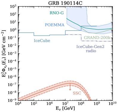
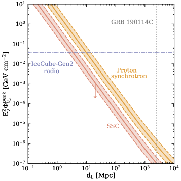
Figure 2: Time-integrated muon neutrino flux expected from the afterglow of GRB 190114C. Left panel: Time-integrated muon neutrino flux for the SSC model (pink shadowed area). This flux represents an upper limit for the real one (for the here considered $\tilde{E}_{k,\rm{iso}}$), as denoted by the pink arrow. The error in the flux prediction is assumed to be a factor $\Delta\Phi_{\nu_{\mu}}/\Phi_{\nu_{\mu}}=\pm 2$, due to the uncertainties in the analytical prescription of the photon flux; see main text. For comparison, the sensitivity of IceCube for a source located at the declination $\delta=-23^{\circ}$ (Abbasi et al., 2021b; Aartsen et al., 2020) is shown as well as the most optimistic ones of IceCube-Gen2 radio for a source at $\delta=0^{\circ}$ (Abbasi et al., 2021b), RNO-G for $\delta=77^{\circ}$ (Aguilar et al., 2021), GRAND200k for a source at $\left|\delta\right|=45^{\circ}$ (Álvarez-Muñiz et al., 2020), and the full-range time-integrated sensitivity of POEMMA (Venters et al., 2020). The neutrino signal lies well below the sensitivity curves of current and upcoming VHE neutrino telescopes. Even though this result depends on the assumed parameters, we expect these conclusions to hold for different sets of parameters within current uncertainties. Right panel: Peak of the time-integrated muon neutrino flux (plotted in the left panel) as a function of the luminosity distance for a bursts with the same properties of GRB 190114C, except for its distance. The arrow for the SSC model is the same as the left panel. For comparison, we show the same result for the proton synchrotron model (yellow shadowed area), by relying on the parameters inferred in Isravel et al. (2022). We also plot the sensitivity of IceCube-Gen2 radio for the optmistic case of a source located at $\delta=0^{\circ}$ (Abbasi et al., 2021b). Note that since the peak of the time-integrated neutrino flux occurs for $E_{\nu}\simeq 10^{7}$–$10^{8}$ GeV for all the redshifts, we approximate the sensitivity of IceCube-Gen2 radio to be constant. In particular, we take the minimum value of the sensitivity to get the most optimistic prediction. For comparison, the dotted grey line indicates GRB 190114C. The peak of the time-integrated neutrino flux becomes comparable to the sensitivity of IceCube-Gen2 radio for $d_{L}\lesssim 5$ Mpc ($d_{L}\lesssim 15$ Mpc) for the SSC model parameters (proton synchrotron). As expected, at each distance the neutrino signal in the case of the proton synchrotron model is larger than the SSC one, since the former naturally requires larger values of $n_{0}$ and $\tilde{E}_{k,\mathrm{iso}}$.

We consider an error band $\Delta\Phi_{\nu_{\mu}}/\Phi_{\nu_{\mu}}=\pm 2$, according to the uncertainties intrinsic to the analytical model, as discussed in Sec. 4.2. The main uncertainties come from the choice of parameters listed in Table 4. Nevertheless, the neutrino signal lies well below the sensitivity curves also for optimistic values of $\varepsilon_{e}$ and $\varepsilon_{B}$—see also Guarini et al. (2022). These findings imply that the non-detection of neutrinos from the afterglow of GRBs with VHE emission is expected and does not allow to further constrain the properties of the bursts. Conversely, detection of VHE neutrinos in coincidence with VHE GRB afterglows would be challenging to explain in the context of the standard afterglow model.

The right panel of Fig. 2 shows the peak of the time-integrated neutrino flux (plotted in the left panel) as a function of the luminosity distance, assuming a burst with properties identical to the ones of GRB 190114C. For comparison, we also show the peak of the time-integrated neutrino flux when the proton synchrotron model is assumed. We rely on the parameters inferred in Isravel et al. (2022). We warn the reader that they are not comparable with the ones obtained in Sec. 4.1 due to our assumption $\xi_{e}=1$ and the requirement $\xi_{e}\ll 1$ for a proton synchrotron model. Hence, the main goal of the right panel of Fig. 2 is to assess whether the neutrino detection perspectives from VHE bursts depend on the selected model for the VHE emission. Since the proton synchrotron model naturally requires larger values of $n_{0}$ and $\tilde{E}_{k,\rm{iso}}$, the resulting neutrino flux is larger than in the SSC scenario.

Comparing the peak of the neutrino flux to the sensitivity of IceCube-Gen2 radio (Abbasi et al., 2021b), which is expected to be the most competitive facility (see left panel), we obtain that the peak of the neutrino flux becomes comparable to the sensitivity of IceCube-Gen2 radio for $d_{L}\lesssim 5$ Mpc ($d_{L}\lesssim 15$ Mpc) for the SSC model parameters (proton synchrotron). Such distances are too small, considering the distribution of long GRBs as a function of the redshift (Jakobsson et al., 2012). Therefore, we conclude that the detection of neutrinos from GRB afterglows displaying VHE emission is not a promising tool to infer GRB properties within a multi-messenger framework. Our conclusions are consistent with the ones of Isravel et al. (2022) for GRB 190114C, which finds that the photo-hadronic interaction rate accounts for inefficient energy extraction.

6 Discussion

Table 5: Summary of the model parameter constraints derived in this work from the afterglow of GRB 180720B, GRB 190114C and GRB 221009A (see also Fig. 1). The range preferred for the kinetic isotropic energy ($\tilde{E}_{k,\rm{iso}}$), the CBM density ($n_{0}\;[A/(3\times 10^{35})]$), and the initial Lorentz factor ($\Gamma_{0,\rm{ISM(wind)}}$) is reported.

GRB	$\tilde{E}_{k,\rm{iso}}$ [erg]	$n_{0}$ or $A/(3\times 10^{35})$	$\Gamma_{0,\rm{ISM}(wind)}$
GRB 180720B	$6\times 10^{53}$–$10^{55}$	$4\times 10^{-5}$–$10^{-1}$ cm-3	$80-1276$
GRB 190114C	$2.5\times 10^{53}$–$10^{55}$	$3\times 10^{-5}$–$2\times 10^{-2}$ cm-3	$50$–$1797$
GRB 221009A	$3\times 10^{54}$–$5\times 10^{55}$	$7\times 10^{-3}$–$10^{-1}$ cm-1	$\lesssim 313$

Our constraints on the VHE GRB properties are summarized in Table 5 for our benchmark bursts, GRB 180720B, GRB 190114C and GRB 221009A (see also Fig. 1). While our sample is small, such findings raise questions on the nature of the progenitors and the sites hosting VHE bursts, if microphysical parameters compatible with the SSC scenario are assumed.

The initial Lorentz factor of our VHE bursts falls within the average expected for GRBs, see Sec. 4.3 and e.g. Secs. 5 and 6 of Ghirlanda et al. (2018). With the caveat that we have observed VHE emission for a few bursts only, our results seem to suggest that these VHE GRBs exhibit isotropic kinetic energy towards the higher tail of the distribution expected for GRBs, see e.g. Fig. 19 of Poolakkil et al. (2021). This result might be biased by the sensitivity of existing telescopes, as well as the viewing angle. In the future, CTA may detect fainter bursts in the VHE regime, providing better insight on the population features and the fraction of GRBs with VHE emission.

As discussed in Sec. 4, VHE GRBs might preferentially occur in a low-density CBM–independently on the microphysics of the shock, the compactness argument requires that $n_{0}\lesssim 1$ cm^-3 and $A/(3\times 10^{35})\lesssim 1$ cm^-1. If microphysical parameters typical of SSC radiation are adopted (e.g., Fraija et al., 2022), even more stringent constraints are obtained. Intriguingly, we reach similar conclusions following the method outlined in Gompertz et al. (2018) that relies on the simplifying assumption that all the bursts can be modelled with the same set of microphysical parameters and have a prompt emission efficiency $\simeq 50\%$. Following Gompertz et al. (2018), we find that the VHE GRBs cluster in the low-density region of the parameter space [$n_{0}(A/(3\times 10^{35}))\lesssim 10^{-1}$ cm^-3 (cm^-1)]. On the contrary, the bursts not displaying VHE emission analyzed in Gompertz et al. (2018) are uniformly distributed in the $(\tilde{E}_{k,\rm{iso}},n)$ space; we refer the interested reader to Appendix C for additional details.

A CBM with low density is usually favored by the synchrotron closure relations (e.g. Gao et al., 2013a), that are found not to be fullfilled for all bursts; hence our findings might be affected by the simplifications intrinsic to these relations. Yet, these results are in agreement with the expectation that low-density environments favor a transparent blastwave in the afterglow. Furthermore, larger densities may reprocess the VHE photons and emit electromagnetic radiation in other wavelengths. In addition, low density CBMs have been associated to long GRBs (e.g. Panaitescu & Kumar, 2002; Gompertz et al., 2018). For example, a wind with $A_{\star}\simeq 4\times 10^{-3}$ has been inferred for GRB 130427A (Panaitescu et al., 2013), as a result of a multi-wavelength fit of the GRB lightcurve. Panaitescu et al. (2013) suggests that the weak wind could be a consequence of the GRB progenitor being hosted in a superbubble (Mirabal et al., 2002; Scalo & Wheeler, 2001). Similarly, Hascoët et al. (2014) finds that the winds of some GRB progenitors are weaker than the ones observed for Wolf-Rayet stars in our Galaxy ($A_{\star}\simeq 1$). This might be linked to the low metallicity of the progenitors (Vink et al., 2001) and their host galaxies (e.g. Perley et al., 2013), which is anyway still under debate (e.g. Perley et al., 2016). Low CBM densities may also be caused by reduced mass-loss rate at the time of the stellar collapse (Hascoët et al., 2014). Recently, Dereli-Bégué et al. (2022) studied bursts with a plateau phase in their afterglow. In order to explain this feature, a small wind density consistent with our findings and a small outflow Lorentz factor are required, the latter implying a lack of VHE (and even HE) emission for those bursts, which Dereli-Bégué et al. (2022) argues is the case.

Our results hold within the assumption that the multi-wavelength radiation is generated by the decelerating blastwave, whose dynamics is outlined in Sec. 3. Such conclusions may substantially change if more complex jet geometries (Sato et al., 2022), time-varying microphysical parameters (Filgas et al., 2011) or two-zone models (Khangulyan et al., 2023) should be invoked, as in the case of GRB 190114C (Misra et al., 2019). Furthermore, low-density CBMs are obtained for $\xi_{e}=1$, whereas smaller fractions of accelerated electrons naturally lead to larger densities (e.g. Isravel et al., 2022). Thus, if a dense CBM should be inferred, e.g. via the SSA frequency in the radio band, it may hint towards a proton synchrotron model. In this sense, determining the CBM density can provide constraints on the mechanism powering the VHE emission. Our results are based on the SSC scenarios, rather than proton synchrotron ones. Since the value of $\xi_{e}$ is largely uncertain, an analysis of the dependence of our conclusions on this parameter is left to future work. Additional input on these parameters may also come from numerical simulations of particle acceleration at the external shock.

Future observations of GRBs in the VHE regime with CTA (Knödlseder, 2020) will be crucial to pinpoint the mechanism powering the VHE emission during the afterglow. However, CTA might have better detection prospects for large CBM surrounding these bursts, as suggested in Mondal et al. (2022). The latter assumes a SSC origin of the VHE emission, although neglecting the cutoff introduced by $\gamma$–$\gamma$ pair production. The SSC efficiency largely depends on the Compton parameter, which is maximized for large blastwave energies and CBM densities. As a consequence, Mondal et al. (2022) obtains CBM densities larger than the ones we infer, since the transparency argument alone is sufficient to limit $n_{0}\lesssim 1$ cm^-3 [$A/(3\times 10^{35})\lesssim 1$ cm^-1]. We stress that the relation used for the opacity argument (Eq. 16) is approximate; therefore, detailed modeling of the energy cutoff and fit to the spectral energy distributions are required to draw robust conclusions from a larger burst sample. Yet, we do not expect the constraint $n<1$ cm^-1 to change drastically.

7 Conclusions

While the number of GRBs detected in the VHE regime during the afterglow will increase in the near future with the advent of CTA, our understanding of the mechanism powering the VHE emission is very preliminary. The standard synchrotron model, which well explains the afterglow data from the radio to the X-ray bands, cannot account for the emission of $\mathcal{O}$(TeV) photons detected at late times.

In this paper, we focus on GRB 180720B, GRB 190114C and GRB 221009A, with the goal to infer the properties of the blastwave and the burst environment. By requiring that the plasma in the blastwave shell is transparent to $\gamma$–$\gamma$ pair production at the time of the observation of the VHE photons, we obtain that the CBM density should be $n_{0}\lesssim 1$ cm³ [$A/(3\times 10^{35})$ cm^-1]. A tentative interpretation of the radio, optical and X-ray data hints towards even lower CBM densities, with $n_{0}\lesssim\mathcal{O}(10^{-1})$ cm^-3 [$A/(3\times 10^{35})\lesssim\mathcal{O}(10^{-1})$ cm^-1], if the microphysical parameters of the shock are taken to be consistent with SSC mechanism. Furthermore, we obtain constraints on the initial Lorentz factor of the blastwave by requiring that the deceleration of the fireball starts before the observation of VHE photons and after the GRB prompt emission, finding $10^{2}\lesssim\Gamma_{0}\lesssim 10^{3}$. While the initial Lorenz factors are within average in the context of long GRBs, we find that (assuming a typical prompt-phase efficiency of $10\%$) the kinetic blastwave energy is large, $\tilde{E}_{k,\rm{iso}}\gtrsim\times\mathcal{O}(10^{54})$ erg (see also Table 5). Albeit such large energies could be due to an observational bias towards detection efficiency. Whether these conclusions are generally valid for VHE GRBs will be confirmed by future CTA observations.

Finally, we investigate the neutrino signal expected from the afterglow of VHE GRBs, focusing on GRB 190114C as representative burst. The non-observation of high-energy neutrinos from VHE GRBs is consistent with our theoretical predictions. The detection prospects for high-energy neutrinos from VHE GRBs with upcoming neutrino telescopes are equally poor, except for bursts closer than $15$ Mpc. This suggests that neutrinos from the GRB afterglow may not be promising messengers to unveil the properties of the VHE emitting bursts.

Our findings hint at arising trends characterizing the properties of VHE GRBs, if the afterglow of these bursts can be modelled within the standard scenario. Additional data on bursts exhibiting VHE emission will shed light on the engine powering such transients and provide valuable insight on the characteristics of their host environments.

Data Availability

Data can be shared upon reasonable request to the authors.

Appendix A Photon energy distribution

The total distribution of target photons is

$$n^{\prime\rm{tot}}_{\gamma}(E^{\prime}_{\gamma})=n^{\prime\rm{sync}}_{\gamma}(E^{\prime}_{\gamma})+n^{\prime\rm{VHE}}_{\gamma}(E^{\prime}_{\gamma})\ ,$$ (21)

where $n^{\prime\rm{sync}}_{\gamma}$ is the synchrotron component defined in Eqs. 12 (including SSC corrections, see Sari & Esin (2001)) and 13 and $n^{\prime\rm{VHE}}_{\gamma}$ is the VHE part of the photon energy distribution.

We model the VHE component of the photon spectrum both with SSC radiatio. The SSC component is obtained by following the prescription in Gao et al. (2013b). We include the Klein-Nishina regime by introducing a cut-off in the photon spectrum at the Klein-Nishina energy (Wang et al., 2019). The latter, can be expressed as Wang et al. (2019):.

$$E_{\rm{KN}}=\left\{\begin{array}[]{@{}l@{}}0.3\;\rm{TeV}\;6\frac{k_{e}-2}{k_{e}-1}\varepsilon_{e,-1}E_{54}^{1/4}n^{-1/4}_{-1}t_{2}^{-3/4}\;\;\;\gamma_{\rm{min}}>\gamma_{\rm{cool}}\\ 0.1\;\rm{TeV}\frac{1}{1+Y}\varepsilon_{B,-2}^{-1}E_{54}^{-1/4}n_{-1}^{-3/4}t_{10\;\rm{hr}}^{-1/4}\;\;\;\;\gamma_{\rm{min}}<\gamma_{\rm{cool}}\;,\end{array}\right.$$ (22)

where $Y$ is the Compton parameter (Sari & Esin, 2001), $\gamma_{\min}$ is given by Eq. 8, while $\gamma_{\rm{cool}}$ is given by dividing Eq. 9 by $1+Y$ (Sari & Esin, 2001). We are using the notation $X_{y}=X/10^{y}$. Therefore, the cutoff $E_{\rm{KN}}$ varies over time and is usually larger at the onset of the afterglow. This is a good approximation, since the VHE photons predominantly interact with low-energy protons, and the neutrinos produced in these interactions do not affect substantially the high-energy neutrino signal.

Appendix B Hadronic interactions

Because of the relatively small baryon density, $pp$ interactions are subleading during the afterglow and only efficient in the innermost regions of the outflow (Razzaque et al., 2003; Metzger et al., 2011; Heinze et al., 2020). Hence, the main channels for neutrino production are

$$p+\gamma \rightarrow \Delta\rightarrow n+\pi^{+},p+\pi^{0}$$ (23)

$$p+\gamma \rightarrow K^{+}+\Lambda/\Sigma\ .$$ (24)

Neutral pions decay into gamma-rays $\pi^{0}\longrightarrow 2\gamma$, while neutrinos are produced through the charged pion decay $\pi^{+}\longrightarrow\nu_{\mu}+\mu^{+}$ followed by $\mu^{+}\longrightarrow\bar{\nu}_{\mu}+\nu_{e}+e^{+}$, and through $n\rightarrow p+e^{-}+\bar{\nu}_{e}$. Antineutrinos are also produced in the corresponding antiparticle channels; however, in this work, we do not distinguish between particle and antiparticles.

B.1 Proton energy distribution

Protons are assumed to be accelerated together with electrons at the forward shock driven by the blastwave in the cold CBM. Their comoving energy distribution is assumed to be [in units of GeV^-1 cm^-3]

$$n^{\prime}_{p}(E^{\prime}_{p})=A^{\prime}_{p}E^{{}^{\prime}-k_{p}}_{p}\exp\biggl{[}-\biggl{(}\frac{E^{\prime}_{p}}{E^{\prime}_{p,\rm{max}}}\biggr{)}^{\alpha_{p}}\biggr{]}\Theta(E^{\prime}_{p}-E^{\prime}_{p,\rm{min}})\ ,$$ (25)

where $\Theta$ is the Heaviside function, $E^{\prime}_{p,\min}=\Gamma m_{p}c^{2}$ (Dermer, 2002; Murase, 2007; Razzaque, 2013) is the minimum energy of accelerated protons and $E^{\prime}_{\max}$ is the maximum energy at which protons can be accelerated. The latter is fixed by equating the acceleration time scale of protons with their total cooling time, which takes into account all the energy loss mechanisms for accelerated protons. We refer the interested reader to Sec. 4 of Guarini et al. (2022) for a detailed discussion.

Finally, $A^{\prime}_{p}=\varepsilon_{p}\xi_{p}u^{\prime}[\int_{E^{\prime}_{p,\min}}^{E^{\prime}_{p,\rm{max}}}dE^{\prime}_{p}E^{\prime}_{p}n^{\prime}_{p}(E^{\prime}_{p})]^{-1}$ is the normalization constant. Here, $u^{\prime}$ is the blastwave energy density defined in Eq. 6, $\varepsilon_{p}\lesssim 1-\varepsilon_{e}-\varepsilon_{B}$ is the fraction of this energy which is stored into accelerated protons and $\xi_{p}$ is the fraction of accelerated protons.

The proton spectral index $k_{p}$ depends on the model invoked for particle acceleration. It is expected to be $k_{p}\simeq 2$ (Matthews et al., 2020) in the non-relativistic shock diffusive acceleration theory, while $k_{p}\simeq 2.2$ is expected from Monte-Carlo simulations of ultra-relativistic shocks (Sironi et al., 2013). The constant $\alpha_{p}=2$ mimics the exponential cutoff in the photon energy distribution (Hümmer et al., 2010).

Appendix C Additional constraints on the properties of the circumburst medium

Both the range of $\tilde{E}_{k,\rm{iso}}$ allowed by the arguments in Sec. 4.2 and the CBM density could span several orders of magnitude. A priori, it is not obvious whether our sample of VHE bursts (despite being based on a small number of bursts) shares common properties in terms of CMB densities with other GRBs without observed VHE emission.

Gompertz et al. (2018) performed a scan of the parameter space allowed for the blastwave isotropic energy and the CBM density for a selected set of GRBs not detected in the VHE regime. We stress that, in this appendix, we assume that our sample of VHE GRBs (Table 1) can be modelled by relying on the same assumptions as in Gompertz et al. (2018) for the microphysical parameters. We also include GRB 130427A observed at $z=0.34$, with $\tilde{E}_{\gamma,\rm{iso}}\simeq 8\times 10^{53}$ erg (Golenetskii et al., 2013; Zhu et al., 2014). Even though this burst has not been detected in the TeV range, it has been observed by Fermi-LAT during the afterglow phase, with photons up to $\mathcal{O}(10)$ GeV about $9$ hours after the trigger (Zhu et al., 2014). Being among the most investigated events of this class, we consider GRB 130427A as representative of the HE sample observed by Fermi-LAT (Ajello et al., 2019).

In light of the existing uncertainties on the microphysical parameters and in order to enable a comparison with the standard bursts of Gompertz et al. (2018) and the VHE ones considered in this work, we relax the values of the microphysical parameters considered in the main text and in Fig. 1. Our goal is to assess whether particular properties are preferred by GRBs emitting VHE photons with respect to standard GRBs.

Once the CBM type is fixed (ISM or wind), following Gompertz et al. (2018), we focus at $11$ hours (as measured on Earth) after the trigger of the burst. At this time, two scenarios are possible: either $\nu_{R}<\nu_{\gamma,\rm{cool}}<\nu_{X}$ or $\nu_{X}<\nu_{\gamma,\rm{cool}}$, where $\nu_{R}$ and $\nu_{X}$ are the observed effective frequencies in the optical $R$ and X-ray bands, respectively. In the former case, we can infer the properties of the blastwave responsible for the afterglow emission (Sari et al., 1998; Pe’er & Waxman, 2005; Gompertz et al., 2018):

$$\frac{\Phi^{\rm{obs}}_{R}}{\Phi^{\rm{obs}}_{{X}}}=\left(\frac{\nu_{R}}{\nu_{X}}\right)^{-k_{e}/2}\nu_{R}^{1/2}\nu_{\gamma,\rm{cool}}^{-1/2}\ ,$$ (26)

where $\Phi^{\rm{obs}}_{R}$ and $\Phi^{\rm{obs}}_{X}$ are the fluxes observed at $11$ hours in the $R$ and X-ray bands, respectively [both in units erg cm^-2 s^-1]. By replacing $\nu_{\gamma,\rm{cool}}$ in Eq. 26 with Eq. 11, we obtain a relation between $\tilde{E}_{k,\rm{iso}}$ and $n_{0}$ or $A/(3\times 10^{35})$.

If $\nu_{X}<\nu_{\gamma,\rm{cool}}$, the blastwave parameters can be inferred from the flux observed in the $R$ band. Plugging $\Phi^{\rm{obs}}_{\nu,R}$ in the left hand side of Eq. 15 and evaluating the right hand side of Eq. 15 at $\nu_{\gamma}\equiv\nu_{R}$ provides us with a relation between $\tilde{E}_{k,\rm{iso}}$ and $n_{0}\;[A/(3\times 10^{35})]$ (Sari et al., 1998; Pe’er & Waxman, 2005); see also Eqs. $6$–$7$ in Gompertz et al. (2018).

The flux in the $R$ band is obtained by converting the AB magnitude through the following relation (Fukugita et al., 1996):

$$m_{\rm{AB}}=-2.5\log_{10}\left(\frac{\Phi^{\rm{obs}}_{\nu,R}}{3631}\right)\ ,$$ (27)

where $\Phi^{\rm{obs}}_{\nu,R}$ is the observed flux [in units of Jy]. The AB magnitudes are extracted from the GCN circular archive (2022). The flux at $11$ hours is extrapolated by evolving $\Phi^{\rm{obs}}_{\nu,R}\propto t^{-\alpha_{O}}$, with $\alpha_{O}$ being the temporal spectral index in the optical band reported in Table 6. Note that these values do not include the intrinsic host galaxy extinction; hence, the value of $\Phi^{\rm{obs}}_{\nu,R}$ that we use is a lower limit of the real flux. We warn the reader that the value of $\alpha_{O}$ obtained for GRB 190114C from the standard closure relations and reported in Table 6 does not reproduce the optical lightcurve and the spectral energy distribution simultaneously and satisfactorily. This hints that the standard afterglow model may not be adequate to model this GRB. Time-varying microphysical parameters might be more appropriate for this burst (Misra et al., 2019); in this case our results would no longer hold.

Table 6: Temporal optical index $\alpha_{O}$ obtained for the three considered VHE bursts and GRB 130427A, with relative References.

Burst	$\alpha_{O}$	References
GRB 180720B	1.2	Fraija et al. (2019c)
GRB 190114C	0.76	Fraija et al. (2019a)
GRB 221009A	0.52	Belkin et al. (2022)
GRB 130427A	1.36	(Panaitescu et al., 2013)

We fix the electron spectral index ($k_{e}$) as indicated in Table 1. In particular, for GRB 190114C we fix the value $k_{e}=2.2$, while we checked that the results are not very sensitive to the variation of $k_{e}$. Furthermore, we assume that the isotropic energy left in the blastwave after the prompt emission is $\tilde{E}_{k,\rm{iso}}\equiv\tilde{E}_{\gamma,\rm{iso}}$ (Gompertz et al., 2018). This implies a prompt efficiency of $\approx 50\%$, which might be optimistic (Beniamini et al., 2016) and should be rather interpreted as a lower limit on $\tilde{E}_{k,\rm{iso}}$.

In both the aforementioned regimes, the microphysical parameters $\varepsilon_{e}$ and $\varepsilon_{B}$ should be fixed. Gompertz et al. (2018) assumes $\varepsilon_{e}=0.1$ and $\varepsilon_{B}=10^{-1}$–$10^{-4}$ for all GRBs in their sample, and they conclude that $\varepsilon_{B}\simeq 10^{-4}$ is preferred to avoid unphysical values of the CBM density. The parameters $\varepsilon_{e}=0.1$ and $\varepsilon_{B}=10^{-5}$–$10^{-4}$ are also consistent with the typical values required for modelling the VHE emission through the SSC mechanism (e.g. Fraija et al., 2022). We first rely on the same choice of the microphysical parameters of Gompertz et al. (2018) to favor a direct comparison between the properties of the VHE bursts and the standard ones and, to this purpose, we use $\varepsilon_{e}=0.1$ and $\varepsilon_{B}=10^{-2}$–$10^{-4}$. Then, we assume $\varepsilon_{B}=10^{-5}$, while keeping $\varepsilon_{e}=0.1$, since this value is allowed in the context of the SSC model. This procedure allows us to obtain upper and lower limits for the CBM densities for the two underlying mechanisms.

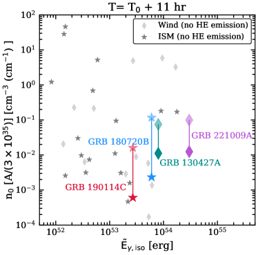
Figure 3: VHE GRBs in Table 1 (each distinguished by a different color) in the plane spanned by the isotropic gamma-ray energy $\tilde{E}_{\gamma,\rm{iso}}$ and CBM density [$n_{0}\;\rm{or}\;A/(3\times 10^{35})$]. Following Gompertz et al. (2018), we fix $\tilde{E}_{k,\rm{iso}}=\tilde{E}_{\gamma,\rm{iso}}$, $\varepsilon_{e}=0.1$ and $\varepsilon_{B}=10^{-4}$–$10^{-5}$ for the lower (opaque markers) and upper limits (shadowed markers), respectively. The stars denote bursts occurring in an ISM, while the diamonds correspond to bursts occurring in a wind-like CBM. The gray stars and diamonds correspond to the bursts analyzed in Gompertz et al. (2018) occurring in an ISM and a wind-like CBM, respectively, for $\varepsilon_{e}=10^{-1}$ and $\varepsilon_{B}=10^{-4}$. The VHE GRBs in our sample favor low density CBM, for $\varepsilon_{B}$ compatible with the SSC model; see main text for details.

Figure 3 summarizes our findings for $\varepsilon_{B}=10^{-5}$–$10^{-4}$. We include GRB 130427A in the plot, as representative of the GRBs detected in the HE regime during the afterglow; see Sec. 2. The results obtained by adopting $\varepsilon_{B}=10^{-4}$ can be directly compared to the ones of Gompertz et al. (2018), as shown in Fig. 3 (gray markers). Intriguingly, the bursts detected in the VHE regime cluster in the region of the parameter space corresponding to large isotropic energy emitted in gamma-rays and relatively small CBM densities [$10^{-3}\lesssim n_{0}\lesssim 10^{-1}$ and $10^{-5}\lesssim A/(3\times 10^{35})\lesssim 10^{-1}$], consistently with our findings displayed in Fig. 1.

The case with $\varepsilon_{B}=10^{-5}$ cannot be compared with the results in Gompertz et al. (2018) directly. Nevertheless, we consider it as representative of the SSC model (Fraija et al., 2022): since $n_{0}\propto\varepsilon_{B}^{-(k_{e}+1)/2}\;[A\propto\varepsilon_{B}^{-(k_{e}+1)/4}]$, we expect the density to increase as $\varepsilon_{B}$ decreases, while keeping fixed $\tilde{E}_{k,\rm{iso}}$. It is worth noticing that decreasing $\varepsilon_{e}$ implies an increase in the CBM density, because $n_{0}\propto\varepsilon_{e}^{(1-k_{e})/2}\;[A\propto\varepsilon_{e}^{(1-k_{e})}]$, for the ISM [wind] scenario. For example, for $\varepsilon_{e}=10^{-2}$ and $\varepsilon_{B}=10^{-2}$, one obtains results similar to the lower limits in Fig. 1. On the contrary, assuming $\varepsilon_{e}=10^{-2}$ and $\varepsilon_{B}=10^{-4}$, shifts the points in Fig. 3 to larger densities, i.e. $n_{0}[A/(3\times 10^{35})]\gtrsim 1$. Nevertheless, the multi-wavelength fits in the literature suggest $\varepsilon_{e}\simeq 0.1$. Hence, the densities obtained in Fig. 3 might be preferred.

We stress that the results in Fig. 3 cannot be directly compared to the ones in Fig. 1, since in the former we fix $\tilde{E}_{k,\rm{iso}}=\tilde{E}_{\gamma,\rm{iso}}$, while in the latter $\tilde{E}_{k,\rm{iso}}$ is a free parameter. In Fig. 1 the scaling of the CBM density with $\varepsilon_{e}$ and $\varepsilon_{B}$ is not trivial, since the isotropic kinetic energy is also changing with the other model parameters.

Note that, $10^{-3}\lesssim\varepsilon_{B}\lesssim 10^{-1}$ (with $\varepsilon_{e}=10^{-1}$) leads to $10^{-8}\lesssim n\;[A/(3\times 10^{35})]\lesssim 10^{-6}$, which is too low to be realistic (Gompertz et al., 2018). This result might be biased by theoretical limitations of the closure relations and by the assumption $\xi_{e}=1$. While the arguments in Sec. 4 are not constraining for GRB 180720B, we conclude from Fig. 3 that low densities might be preferred for VHE bursts for typical microphysical parameters consistent with a SSC scenario, as also found in Wang et al. (2019).

References

- Aartsen et al. (2017) Aartsen M. G., et al., 2017, Astrophys. J., 843, 112
- Aartsen et al. (2020) Aartsen M. G., et al., 2020, Astrophys. J. Lett., 898, L10
- Abbasi et al. (2021a) Abbasi R., et al., 2021a, arXiv e-prints, p. arXiv:2101.09836
- Abbasi et al. (2021b) Abbasi R., et al., 2021b, PoS, ICRC2021, 1183
- Abbasi et al. (2022a) Abbasi R., et al., 2022a, Eur. Phys. J. C, 82, 1031
- Abbasi et al. (2022b) Abbasi R., et al., 2022b, Astrophys. J., 939, 116
- Abdalla et al. (2019) Abdalla H., et al., 2019, Nature, 575, 464
- Abdalla et al. (2021) Abdalla H., et al., 2021, Science, 372, 1081
- Acciari et al. (2019a) Acciari V. A., et al., 2019a, Nature, 575, 455
- Acciari et al. (2019b) Acciari V. A., et al., 2019b, Nature, 575, 459
- Aguilar et al. (2021) Aguilar J. A., et al., 2021, JINST, 16, P03025
- Aharonian et al. (2023) Aharonian F., et al., 2023, arXiv e-prints
- Ai & Gao (2023) Ai S., Gao H., 2023, Astrophys. J., 944, 115
- Ajello et al. (2019) Ajello M., et al., 2019, Astrophys. J., 878, 52
- Álvarez-Muñiz et al. (2020) Álvarez-Muñiz J., et al., 2020, Sci. China Phys. Mech. Astron., 63, 219501
- Asano et al. (2009) Asano K., Inoue S., Meszaros P., 2009, Astrophys. J., 699, 953
- Asano et al. (2020) Asano K., Murase K., Toma K., 2020, Astrophys. J., 905, 105
- Atteia et al. (2017) Atteia J. L., et al., 2017, Astrophys. J., 837, 119
- Baring & Harding (1997) Baring M. G., Harding A. K., 1997, Astrophys. J., 491, 663
- Belkin et al. (2022) Belkin S., Pozanenko A., Klunko E., Pankov N., GRB IKI FuN 2022, GRB Coordinates Network, 32645, 1
- Beniamini et al. (2016) Beniamini P., Nava L., Piran T., 2016, Mon. Not. Roy. Astron. Soc., 461, 51
- Blandford & McKee (1976) Blandford R. D., McKee C. F., 1976, Physics of Fluids, 19, 1130
- Bottcher & Dermer (1998) Bottcher M., Dermer C. D., 1998, Astrophys. J. Lett., 499, L131
- Chevalier & Li (1999) Chevalier R. A., Li Z. Y., 1999, Astrophys. J. Lett., 520, L29
- Chevalier & Li (2000) Chevalier R. A., Li Z.-Y., 2000, Astrophys. J., 536, 195
- Chiang & Dermer (1999) Chiang J., Dermer C. D., 1999, Astrophys. J., 512, 699
- Crowther (2007) Crowther P. A., 2007, Ann. Rev. Astron. Astrophys., 45, 177
- Dai & Lu (1998) Dai Z. G., Lu T., 1998, Mon. Not. Roy. Astron. Soc., 298, 87
- Dereli-Bégué et al. (2022) Dereli-Bégué H., Pe’er A., Ryde F., Oates S. R., Zhang B., Dainotti M. G., 2022, Nature Commun., 13, 5611
- Derishev & Piran (2021) Derishev E., Piran T., 2021, Astrophys. J., 923, 135
- Dermer (2002) Dermer C. D., 2002, Astrophys. J., 574, 65
- Dermer et al. (2000) Dermer C. D., Chiang J., Mitman K. E., 2000, Astrophys. J., 537, 785
- Eichler & Waxman (2005) Eichler D., Waxman E., 2005, Astrophys. J., 627, 861
- Farah et al. (2022) Farah W., Bright J., Pollak A., Siemion A., DeBoer D., Fender R., Rhodes L., Heywood I., 2022, GRB Coordinates Network, 32655, 1
- Filgas et al. (2011) Filgas R., et al., 2011, Astron. Astrophys., 535, A57
- Ford et al. (1995) Ford L. A., et al., 1995, Astrophys. J., 439, 307
- Fraija et al. (2019a) Fraija N., Dichiara S., Caligula do E. S. Pedreira A. C., Galvan-Gamez A., Becerra R. L., Barniol Duran R., Zhang B. B., 2019a, Astrophys. J. Lett., 879, L26
- Fraija et al. (2019b) Fraija N., Duran R. B., Dichiara S., Beniamini P., 2019b, Astrophys. J., 883, 162
- Fraija et al. (2019c) Fraija N., et al., 2019c, Astrophys. J., 885, 29
- Fraija et al. (2022) Fraija N., Dainotti M. G., Ugale S., Jyoti D., Warren D. C., 2022, Astrophys. J., 934, 188
- Frederiks et al. (2018) Frederiks D., et al., 2018, GRB Coordinates Network, 23011, 1
- Frederiks et al. (2020) Frederiks D., et al., 2020, GRB Coordinates Network, 29084, 1
- Frederiks et al. (2022) Frederiks D., Lysenko A., Ridnaia A., Svinkin D., Tsvetkova A., Ulanov M., Cline T., Konus-Wind Team 2022, GRB Coordinates Network, 32668, 1
- Fukami et al. (2021) Fukami S., et al., 2021, PoS, ICRC2021, 788
- Fukugita et al. (1996) Fukugita M., Ichikawa T., Gunn J. E., Doi M., Shimasaku K., Schneider D. P., 1996, Astron. J., 111, 1748
- GCN circular archive (2022) GCN circular archive 2022, The Gamma-Ray Coordinates Network, https://gcn.gsfc.nasa.gov/gcn/gcn3_archive.html
- Gagliardini et al. (2022) Gagliardini S., Celli S., Guetta D., Zegarelli A., Capone A., Campion S., Di Palma I., 2022, arXiv e-prints, p. arXiv:2209.01940
- Gao et al. (2012) Gao S., Asano K., Mészáros P., 2012, JCAP, 2012, 058
- Gao et al. (2013a) Gao H., Lei W.-H., Zou Y.-C., Wu X.-F., Zhang B., 2013a, New Astron. Rev., 57, 141
- Gao et al. (2013b) Gao H., Lei W.-H., Wu X.-F., Zhang B., 2013b, Mon. Not. Roy. Astron. Soc., 435, 2520
- Gehrels et al. (2009) Gehrels N., Ramirez-Ruiz E., Fox D. B., 2009, Ann. Rev. Astron. Astrophys., 47, 567
- Ghirlanda et al. (2018) Ghirlanda G., et al., 2018, Astron. Astrophys., 609, A112
- Ghisellini & Celotti (1999) Ghisellini G., Celotti A., 1999, Astrophys. J. Lett., 511, L93
- Golenetskii et al. (2013) Golenetskii S., et al., 2013, GRB Coordinates Network, 14487, 1
- Gompertz et al. (2018) Gompertz B. P., Fruchter A. S., Pe’er A., 2018, Astrophys. J., 866, 162
- Gropp et al. (2019) Gropp J. D., et al., 2019, GRB Coordinates Network, 23688, 1
- Guarini et al. (2022) Guarini E., Tamborra I., Bégué D., Pitik T., Greiner J., 2022, JCAP, 06, 034
- Hamburg et al. (2019) Hamburg R., Veres P., Meegan C., Burns E., Connaughton V., Goldstein A., Kocevski D., Roberts O. J., 2019, GRB Coordinates Network, 23707, 1
- Hascoët et al. (2012) Hascoët R., Daigne F., Mochkovitch R., Vennin V., 2012, Mon. Not. Roy. Astron. Soc., 421, 525
- Hascoët et al. (2014) Hascoët R., Beloborodov A. M., Daigne F., Mochkovitch R., 2014, Astrophys. J., 782, 5
- Heinze et al. (2020) Heinze J., Biehl D., Fedynitch A., Boncioli D., Rudolph A., Winter W., 2020, Mon. Not. Roy. Astron. Soc., 498, 5990
- Huang et al. (2022) Huang Y., Hu S., Chen S., Zha M., Liu C., Yao Z., Cao Z., Experiment T. L., 2022, GRB Coordinates Network, 32677, 1
- Hümmer et al. (2010) Hümmer S., Ruger M., Spanier F., Winter W., 2010, Astrophys. J., 721, 630
- IceCube Collaboration (2022) IceCube Collaboration 2022, GRB Coordinates Network, 32665, 1
- Isravel et al. (2022) Isravel H., Pe’er A., Bégué D., 2022, arXiv e-prints, p. arXiv:2210.02363
- Jakobsson et al. (2012) Jakobsson P., et al., 2012, Astrophys. J., 752, 62
- Kann & Agui Fernandez (2022) Kann D. A., Agui Fernandez J. F., 2022, GRB Coordinates Network, 32762, 1
- Katz & Piran (1997) Katz J. I., Piran T., 1997, Astrophys. J., 490, 772
- Khangulyan et al. (2023) Khangulyan D., Taylor A. M., Aharonian F., 2023, arXiv e-prints, p. arXiv:2301.08578
- Klebesadel et al. (1973) Klebesadel R. W., Strong I. B., Olson R. A., 1973, Astrophys. J. Lett., 182, L85
- Knödlseder (2020) Knödlseder J., 2020, arXiv e-prints, p. arXiv:2004.09213
- Kumar & Zhang (2014) Kumar P., Zhang B., 2014, Phys. Rept., 561, 1
- Laskar et al. (2023) Laskar T., et al., 2023, Astrophys. J. Lett., 946, L23
- Lesage et al. (2022) Lesage S., Veres P., Roberts O. J., Burns E., Bissaldi E., Fermi GBM Team 2022, GRB Coordinates Network, 32642, 1
- Levinson & Nakar (2020) Levinson A., Nakar E., 2020, Phys. Rept., 866, 1
- Li et al. (2002) Li Z., Dai Z. G., Lu T., 2002, Astron. Astrophys., 396, 303
- Li et al. (2023) Li L., et al., 2023, Astrophys. J. Lett., 944, L57
- Lithwick & Sari (2001) Lithwick Y., Sari R., 2001, Astrophys. J., 555, 540
- Liu et al. (2013) Liu R.-Y., Wang X.-Y., Wu X.-F., 2013, Astrophys. J. Lett., 773, L20
- Liu et al. (2022) Liu R.-Y., Zhang H.-M., Wang X.-Y., 2022, arXiv e-prints, p. arXiv:2211.14200
- Lucarelli et al. (2022) Lucarelli F., Oganesyan G., Montaruli T., Branchesi M., Mei A., Ronchini S., Brighenti F., Banerjee B., 2022, arXiv e-prints, p. arXiv:2208.13792
- Matthews et al. (2020) Matthews J., Bell A., Blundell K., 2020, New Astron. Rev., 89, 101543
- Meszaros (2002) Meszaros P., 2002, Ann. Rev. Astron. Astrophys., 40, 137
- Meszaros & Rees (1997) Meszaros P., Rees M. J., 1997, Astrophys. J., 476, 232
- Meszaros et al. (1994) Meszaros P., Rees M. J., Papathanassiou H., 1994, Astrophys. J., 432, 181
- Metzger et al. (2011) Metzger B. D., Giannios D., Horiuchi S., 2011, Mon. Not. Roy. Astron. Soc., 415, 2495
- Mirabal et al. (2002) Mirabal N., et al., 2002, Astrophys. J., 578, 818
- Misra et al. (2019) Misra K., et al., 2019, Mon. Not. Roy. Aastron. Soc., 504, 5685
- Mondal et al. (2022) Mondal T., Pramanick S., Resmi L., Bose D., 2022, arXiv e-prints, p. arXiv:2212.07874
- Murase (2007) Murase K., 2007, Phys. Rev. D, 76, 123001
- Murase et al. (2022) Murase K., Mukhopadhyay M., Kheirandish A., Kimura S. S., Fang K., 2022, Astrophys. J. Lett., 941, L10
- Nakar et al. (2009) Nakar E., Ando S., Sari R., 2009, Astrophys. J., 703, 675
- Panaitescu & Kumar (2000) Panaitescu A., Kumar P., 2000, Astrophys. J., 543, 66
- Panaitescu & Kumar (2002) Panaitescu A., Kumar P., 2002, Astrophys. J., 571, 779
- Panaitescu et al. (2013) Panaitescu A., Vestrand W. T., Wozniak P., 2013, Mon. Not. Roy. Astron. Soc., 436, 3106
- Pe’er & Waxman (2005) Pe’er A., Waxman E., 2005, Astrophys. J., 633, 1018
- Perley et al. (2013) Perley D. A., et al., 2013, Astrophys. J., 778, 128
- Perley et al. (2016) Perley D. A., et al., 2016, Astrophys. J., 817, 8
- Piran (2004) Piran T., 2004, Rev. Mod. Phys., 76, 1143
- Poolakkil et al. (2021) Poolakkil S., et al., 2021, Astrophys. J., 913, 60
- Razzaque (2013) Razzaque S., 2013, Phys. Rev. D, 88, 103003
- Razzaque et al. (2003) Razzaque S., Meszaros P., Waxman E., 2003, Phys. Rev. D, 68, 083001
- Razzaque et al. (2010) Razzaque S., Dermer C. D., Finke J. D., 2010, Open Astron. J., 3, 150
- Ren et al. (2022) Ren J., Wang Y., Zhang L.-L., 2022, arXiv e-prints, p. arXiv:2210.10673
- Roberts & Meegan (2018) Roberts O. J., Meegan C., 2018, GRB Coordinates Network, 22981, 1
- Rudolph et al. (2023) Rudolph A., Petropoulou M., Winter W., Bošnjak Ž., 2023, Astrophys. J. Lett., 944, L34
- Sahu & López Fortín (2020) Sahu S., López Fortín C. E., 2020, Astrophys. J. Lett., 895, L41
- Sahu et al. (2022) Sahu S., Polanco I. A. V., Rajpoot S., 2022, Astrophys. J., 929, 70
- Sari & Esin (2001) Sari R., Esin A. A., 2001, Astrophys. J., 548, 787
- Sari et al. (1998) Sari R., Piran T., Narayan R., 1998, Astrophys. J. Lett., 497, L17
- Sato et al. (2022) Sato Y., Murase K., Ohira Y., Yamazaki R., 2022, arXiv e-prints
- Scalo & Wheeler (2001) Scalo J., Wheeler J. C., 2001, Astrophys. J., 562, 664
- Schulze et al. (2011) Schulze S., et al., 2011, in McEnery J. E., Racusin J. L., Gehrels N., eds, American Institute of Physics Conference Series Vol. 1358, Gamma Ray Bursts 2010. pp 165–168, doi:10.1063/1.3621763
- Sfaradi et al. (2018) Sfaradi I., Bright J., Horesh A., Fender R., Motta S., Titterington D., Perrott Y., 2018, GRB Coordinates Network, 23037, 1
- Sironi et al. (2013) Sironi L., Spitkovsky A., Arons J., 2013, Astrophys. J., 771, 54
- Suda et al. (2021) Suda Y., et al., 2021, PoS, ICRC2021, 797
- Venters et al. (2020) Venters T. M., Reno M. H., Krizmanic J. F., Anchordoqui L. A., Guépin C., Olinto A. V., 2020, Phys. Rev. D, 102, 123013
- Vietri (1995) Vietri M., 1995, Astrophys. J., 453, 883
- Vink et al. (2001) Vink J. S., de Koter A., Lamers H. J. G. L. M., 2001, Astron. Astrophys., 369, 574
- Wang et al. (2019) Wang X.-Y., Liu R.-Y., Zhang H.-M., Xi S.-Q., Zhang B., 2019, Astrophys. J., 884, 117
- Warren et al. (2018) Warren D. C., Barkov M. V., Ito H., Nagataki S., Laskar T., 2018, Mon. Not. Roy. Astron. Soc., 480, 4060
- Waxman (1995) Waxman E., 1995, Phys. Rev. Lett., 75, 386
- Waxman (1997a) Waxman E., 1997a, Astrophys. J. Lett., 485, L5
- Waxman (1997b) Waxman E., 1997b, Astrophys. J. Lett., 489, L33
- Waxman (1997c) Waxman E., 1997c, Astrophys. J. Lett., 491, L19
- Waxman (2000) Waxman E., 2000, Phys. Scripta T, 85, 117
- Xia et al. (2022) Xia Z.-Q., Wang Y., Yuan Q., Fan Y.-Z., 2022, GRB Coordinates Network, 32748, 1
- Zhang (2018) Zhang B., 2018, The Physics of Gamma-Ray Bursts. Cambridge University Press, doi:10.1017/9781139226530
- Zhu et al. (2014) Zhu S., Chiang J., Dermer C., Omodei N., Vianello G., Xiong S., Fermi-LAT t., 2014, Science, 343, 42
- Zyla et al. (2020) Zyla P. A., et al., 2020, PTEP, 2020, 083C01
- de Ugarte Postigo et al. (2022) de Ugarte Postigo A., et al., 2022, GRB Coordinates Network, 32648, 1
- Swift Burst Analyser (2022) Swift Burst Analyser 2022, BAT-XRT-UVOT light curves, https://www.swift.ac.uk/burst_analyser/
- von Kienlin et al. (2020) von Kienlin A., et al., 2020, Astrophys. J., 893, 46