Probing the pulsar explanation of the Galactic-Center GeV excess using continuous gravitational-wave searches

Abstract

Over ten years ago, Fermi observed an excess of GeV gamma rays from the Galactic Center whose origin is still under debate. One explanation for this excess involves annihilating dark matter; another requires an unresolved population of millisecond pulsars concentrated at the Galactic Center. In this work, we use the results from LIGO/Virgo’s most recent all-sky search for quasi-monochromatic, persistent gravitational-wave signals from isolated neutron stars, which is estimated to be about 20-50% of the population, to determine whether unresolved millisecond pulsars could actually explain this excess. First, we choose a luminosity function that determines the number of millisecond pulsars required to explain the observed excess. Then, we consider two models for deformations on millisecond pulsars to determine their ellipticity distributions, which are directly related to their gravitational-wave radiation. Lastly, based on null results from the O3 Frequency-Hough all-sky search for continuous gravitational waves, we find that a large set of the parameter space in the pulsar luminosity function can be excluded. We also evaluate how these exclusion regions may change with respect to various model choices. Our results are the first of their kind and represent a bridge between gamma-ray astrophysics, gravitational-wave astronomy, and dark-matter physics.

I Introduction

A tantalizing excess of GeV gamma rays was observed by Fermi over 10 years ago coming from the Galactic Center, and yet its origin has remained elusive. While early studies suggested that the almost spherically symmetric Galactic-Center excess spatial morphology was well-fit by dark-matter models Goodenough and Hooper (2009); Hooper and Goodenough (2011); Hooper and Linden (2011); Gordon and Macias (2013); Daylan et al. (2016); Calore et al. (2015a); Abazajian et al. (2014), and that recent cosmic-ray burst events in our galaxy could also explain this excess Petrović et al. (2014); Carlson and Profumo (2014); Cholis et al. (2015a), an astrophysical explanation of unresolved millisecond pulsars also appears consistent with the observed excess Abazajian (2011); Calore et al. (2015b); Yuan and Zhang (2014); Petrović et al. (2015); Ye and Fragione (2022). The debate between these two explanations is intense: some studies claim that the spatial morphology of the Galactic-Center excess matches better with the mass distribution of the galactic bulge Macias et al. (2018); Bartels et al. (2018); Macias et al. (2019); Pohl et al. (2022), while other studies indicate a preference for a spherically symmetric distribution Di Mauro (2021); Cholis et al. (2022). There have also been potential detections of gamma rays from point sources in the inner Galaxy Lee et al. (2015, 2016); Buschmann et al. (2020), but it was shown recently that systematic biases favoring individual sources may exist in these works Leane and Slatyer (2019, 2020a, 2020b). Furthermore, predictions for the fraction of the Galactic-Center excess explained by millisecond pulsars range from a few percent Hooper et al. (2013); Hooper and Linden (2016) to 100% Ploeg et al. (2020), depending on the luminosity function chosen.

The general theme behind these studies is to devise a luminosity function to fit the observed Galactic-Center excess, based on minimal assumptions Bartels et al. (2018); List et al. (2021) or astrophysics, e.g. assuming luminosity functions identical to those from known millisecond pulsars in globular clusters Hooper and Linden (2016), asserting that accretion-induced collapse is responsible for creating a millisecond pulsar population Gautam et al. (2022), or allowing emissions from low-mass X-ray binaries to compose the Galactic-Center excess Cholis et al. (2015b); Haggard et al. (2017). However, since these choices are required to generate the same observed excess, only some studies of X-rays Berteaud et al. (2021), TeV gamma-rays Macias et al. (2021) and radio observations Calore et al. (2016) have allowed to actually exclude luminosity functions.

Another approach is thus needed to test the viability of the millisecond pulsar hypothesis. In this paper, we show that all-sky searches for continuous waves, i.e. quasi-monochromatic, persistent signals from isolated, asymmetrically rotating neutron stars concentrated around the Galactic Center, can constrain the millisecond pulsar hypothesis for a chosen luminosity function and provide a complementary probe of the Galactic-Center excess.

Gravitational waves could be emitted by neutron stars with deformations on their surfaces, which would then cause a “spin-down”, a decrease in the rotational frequency of the star over time, of $\mathcal{O}(<10^{-9})$ Hz/s. The size of this deformation is a priori unknown and could vary amongst neutron stars Woan et al. (2018); however, contrary to Fermi, advanced LIGO Aasi et al. (2015), Virgo Acernese et al. (2014) and KAGRA Aso et al. (2013) do not rely on electromagnetic emissions, meaning they could potentially detect gravitational waves from sources Fermi may not see.

In fact, the strength of a superposition of signals from a stochastic gravitational-wave background of isolated millisecond pulsars in the Galactic Center was calculated in Calore et al. (2019), assuming a fixed ellipticity and moment of inertia for the population. However, the authors did not systematically try to exclude the luminosity function, nor test robustness of their calculations against different modeling assumptions for the millisecond pulsar population. Furthermore, a stochastic gravitational-wave background was actually searched for in the Galactic Center recently Agarwal et al. (2022), resulting in constraints on the ellipticity of millisecond pulsars there; however, this search was conducted independently of any knowledge of the GeV excess. In contrast, here we consider millisecond pulsars emitting individually-detectable signals, directly link gravitational-wave searches and the observed luminosity of the GeV excess, and put data-driven constraints, while testing the robustness of our modeling choices.

To address the Galactic-Center excess problem using gravitational waves, we will use results from one of the most recent all-sky searches of the latest LIGO/Virgo/KAGRA data, O3, that targeted isolated neutron stars with gravitational-wave frequencies between [10, 2048] Hz and spin-downs between $[-10^{-9},+10^{-8}$] Hz/s Abbott et al. (2022a) with the Frequency-Hough method Astone et al. (2014). We will specifically consider the portion of the sky that contains the Galactic Center. Additionally, we choose to use upper limits from searches for isolated neutron stars because these searches can reach the Galactic Center ($\sim$ 8 kpc), which cannot yet be reached by all-sky searches for neutron stars in binary systems, thus our results only constrain isolated millisecond pulsars that could comprise $\sim 20\%$ of the population Jiang et al. (2020), and some binary systems with particular orbital parameters– see App. D.

II Millisecond pulsars

II.1 Gravitational-wave emission

Gravitational waves from an isolated neutron star could be emitted due to a deviation from axial symmetry, which can be written in terms of a dimensionless equatorial ellipticity $\epsilon$, defined in terms of the star’s principal moments of inertia Maggiore (2008) $\epsilon\equiv{|I_{\rm xx}-I_{\rm yy}|}/{I_{\rm zz}}$. The value of $I_{\rm zz}$ is at $\mathcal{O}(10^{38}-10^{39})$ kg$\cdot$m², depending on the unknown neutron star equation of state Steiner et al. (2015); Breu and Rezzolla (2016). In this study, we choose three representative values $(10^{38},5\times 10^{38},10^{39})$kg m². The gravitational-wave amplitude $h_{0}$ is directly proportional to the ellipticity Maggiore (2008):

$$h_{0}=\frac{16\pi^{2}G}{c^{4}}\frac{I_{\rm zz}\epsilon f_{\rm rot}^{2}}{d},$$ (1)

where $d$ is the star’s distance from the Earth, $f_{\rm rot}$ is the star’s rotational frequency.

We plot a distribution of gravitational-wave frequencies given by the Australian Telescope National Facility (ATNF) catalog Manchester et al. (2005) in App. A. In this study, we adopt the strategy in De Lillo et al. (2022) and assume this distribution of frequencies is representative of the unknown rotational frequencies of millisecond pulsars.

It is also useful to introduce the spin-down limit ellipticity $\epsilon^{\rm sd}$. This is the maximum allowed ellipticity of a neutron star, assuming that all of the rotational energy lost by a millisecond pulsar is converted into gravitational waves Abbott et al. (2021b):

$$\epsilon^{\rm sd}=\sqrt{\frac{5c^{5}}{2G}}\frac{1}{16\pi^{2}}\sqrt{\frac{|\dot{f}_{\rm rot}|}{I_{\rm zz}f_{\rm rot}^{5}}}.$$ (2)

In the following study, we consider two models to determine the ellipticity distribution of millisecond pulsars. The first is to model the deformation as being caused by a strong internal magnetic field misaligned with the star’s rotational axis Lander et al. (2012); Mastrano and Melatos (2012); Lander (2014). The second is to require that the gravitational-wave radiation of millisecond pulsars is a fixed fraction of the total energy loss Ushomirsky et al. (2000); Horowitz and Kadau (2009).

II.2 Deformation caused by magnetic field

Neutron stars cannot remain spherical in the presence of a strong internal magnetic field, $B_{\rm int}$ Maggiore (2018); Chandrasekhar and Fermi (1953). If this field does not align with the rotational axis, it could sustain a deformation on the surface. Specifically, assuming a superconducting core, the ellipticity is related to $B_{\rm int}$ as Abbott et al. (2020), $\epsilon\approx 10^{-8}\left(\frac{B_{\rm int}}{10^{12}\,\rm Gs}\right)$.

The internal magnetic field of a pulsar is not directly observable. We have to derive its value using the pulsar’s measured external magnetic field, $B_{\rm ext}$. In this study, we consider a range of ratios when calculating the probability of gravitational-wave detection based on O3 search results, but we take a benchmark value as $B_{\rm int}=150B_{\rm ext}$, motivated by Ciolfi and Rezzolla (2013); Haskell et al. (2015), when applying our results to exclude portions of the luminosity function parameter space (see Sec. III and Sec. IV). We also assume millisecond pulsars near the Galactic Center follow the same $B_{\rm ext}$ distribution given in the ATNF catalog Manchester et al. (2005). However, the internal magnetic field could even be $10^{4}$ times larger than the external one Vigelius and Melatos (2009); Priymak et al. (2011).

In App. A, we show the probability distribution of ellipticity, assuming an external magnetic field distribution reported in the ATNF catalog.

II.3 Fixed fraction of gravitational-wave energy loss

Rather than relying on specific models to estimate the ellipticity distribution, we also employ ellipticities that are inferred from the ATNF catalog at $\sim 5\%$ or $\sim 10\%$ of the spin-down limit. Such a choice is motivated by recent constraints on the gravitational-wave equatorial ellipticities of millisecond pulsars, in which the spin-down limit has been slightly surpassed for some known millisecond pulsars Abbott et al. (2020). We note that our assumed values are smaller with respect to the constraints on millisecond pulsars in Abbott et al. (2020) This probability density distribution is given in App. A.

II.4 Luminosity function for galactic-center GeV emission

The luminosity function is directly related to the number of millisecond pulsars needed to explain the observed GeV excess, and is one of the dominant contributions to astrophysical uncertainties. In this paper, we use two well accepted benchmarks. The first is a luminosity function following a log-normal distribution  Hooper and Linden (2016):

$$\frac{dN}{dL}\propto\frac{dP(L)}{dL}=\frac{\log_{10}e}{\sigma_{L}\sqrt{2\pi}L}\exp{\left(-\frac{{\log_{10}^{2}(L/L_{0})}}{2\sigma_{L}^{2}}\right)},$$ (3)

where $L$ is the luminosity, and $L_{0}$ and $\sigma_{L}$ are two free parameters. Details on the ranges of these parameters are given in App. B.

The second benchmark has a general power-law dependence on energy cut ($E_{\rm cut}$), magnetic field ($B$) and the spin-down power ($\dot{E}$) Ploeg et al. (2020):

$$L\frac{dP(L)}{dL}=\eta E_{\rm cut}^{a_{\gamma}}B^{b_{\gamma}}\dot{E}^{d_{\gamma}}.$$ (4)

More detailed discussion of this luminosity function can be found in App. B.

We note that our results can easily be generalized to different luminosity functions, since the result from the gravitational-wave search simply translates to a constraint on the total number of millisecond pulsars detectable via gravitational waves, i.e. $N_{\rm GW}$. For a different choice of the pulsar luminosity function, one simply needs to compare $N_{\rm GW}$ with the number of pulsars needed to explain the GeV excess to obtain a constraint on the luminosity function parameters.

Following the discussion in Dinsmore and Slatyer (2022), we first calculate the total luminosity contributed by millisecond pulsars in the Galactic Center:

$$L_{\text{GCE}}=N_{\text{MSP}}\int_{L_{\text{min}}}^{\infty}LP(L)dL.$$ (5)

Here $N_{\text{MSP}}$ is an overall normalization parameter, characterizing the number of millisecond pulsars, and $L_{\rm min}$ is the minimum detectable luminosity by Fermi. For $L_{\rm GCE}\approx 10^{37}$ erg/s (see App. B for how we obtain this number), we compute $N_{\rm MSP}$ for various choices of $L_{0}$ and $\sigma_{L}$, which will influence the number of detectable gravitational-wave sources in O3.

III Method

A search for quasi-monochromatic gravitational-wave signals originating from anywhere in the sky was performed using data from the third observing run of advanced LIGO/Virgo/KAGRA Abbott et al. (2022a). One algorithm, the Frequency-Hough Astone et al. (2014), tracks linear frequency evolution over time by mapping points in the time-frequency plane of the detector to lines in the frequency/frequency derivative plane of the source Astone et al. (2014); Piccinni et al. (2019). Though all outliers were vetoed, competitive upper limits were set on the degree of deformation that neutron stars could have – see App. C.

In this study, we apply the results obtained in the Frequency-Hough all-sky search to calculate the number of detectable millisecond pulsars at the Galactic Center. We note that this search and the one that specifically targets a single sky pixel that completely covers the Galactic Center Abbott et al. (2022b) are complementary to each other, and we will comment on the future optimization later. The Galactic-Center search can obtain a better sensitivity than the all-sky one, since it only looks at one pixel, significantly reducing the computational cost of the search, and can therefore use longer Fourier Transforms to look for quasi-monochromatic signals. Here, however, we would like to consider a larger spatial extent than that covered in the Galactic-Center search, i.e. greater than 150 pc from the Galactic Center, which is why we use the all-sky search results. We therefore apply a correction factor to “specialize” the all-sky search results to the Galactic Center, as described in App. C.

In our study, we assume particular ellipticity distributions described in Sec. II.2 and II.3. Furthermore, we apply the rotation frequency distribution measured in the ATNF catalog Manchester et al. (2005) to determine the gravitational-wave frequency from these millisecond pulsars, as shown in App. A. We provide details on the conversion from the direct output of the gravitational-wave search, $h_{0}$, to the ellipticity $\epsilon$ in App. C.

Let us calculate the probability for a millisecond pulsar to be detectable through gravitational-wave measurements, $P_{\rm GW}$. The gravitational-wave search leads to upper limits of the ellipticity as a function of the frequency, i.e. $\epsilon_{\rm UL}(f)$, at a given confidence level (here, 95%). These limits mean that if there is one millisecond pulsar whose rotation frequency is $f_{\rm rot}$ and ellipticity is larger than $\epsilon_{\rm UL}(f)$, it should have been detected by the search. As an illustration, we present the results for the Frequency-Hough all-sky search in App. C. From these upper limits in App. C, we first calculate the probability that a neutron star has an ellipticity above the minimum detectable one for a given frequency. This is obtained by integrating the ellipticity distribution, given in Fig. 4 or 5, over the value above $\epsilon_{\rm UL}(f)$. We then integrate this quantity over the frequency distribution given in Fig. 3. This gives

$$P_{\rm GW} = \int_{\log_{10}f_{\rm min}}^{\log_{10}f_{\rm max}}d\log_{10}fP(\log_{10}f)$$ (6)

$$\times \int_{\log_{10}\epsilon{{}_{\rm UL}}}^{0}d\log_{10}\epsilon P(\log_{10}\epsilon)$$

where $P(\log_{10}f)$ and $P(\log_{10}\epsilon)$ are the probability density functions for gravitational wave frequency and ellipticity, respectively, and $f$ has units of Hz. Also, we take $f_{\rm min}=120$ Hz and $f_{\rm max}=2000$ Hz, which is in the range of frequencies analyzed in the all-sky search Abbott et al. (2022b) with a cutoff at $f_{\rm rot}=60$ Hz to ensure we are targeting millisecond pulsars. The distributions over ellipticity and frequency are normalized to one and assumed to be independent.

At last, the number of millisecond pulsars detectable with gravitational waves $N_{\rm GW}$ can be easily determined as $N_{\rm GW}=P_{\rm GW}N_{\rm MSP}$, where $N_{\rm MSP}$ is obtained in Sec. II.4. If a set of luminosity function parameters $L_{0}$ and $\sigma_{L}$ leads to $N_{\rm GW}\geq 1$, it indicates that the Frequency-Hough all-sky search should have observed at least one millisecond pulsar in the population if those $L_{0}$ and $\sigma_{L}$ did explain the GeV excess. Consequently, such a set should be excluded.

IV Results

$P_{\rm GW}$ is fixed by the frequency and ellipticity distributions that we choose, as well as the upper limits on ellipticity from the Frequency-Hough all-sky search. It is therefore independent of the luminosity function model considered to explain the GeV excess. Thus, we first present our results in terms of $P_{\rm GW}$ which can be directly applied to probe the parameter space of any luminosity function. Here, we provide, in the left- and right- hand side of Fig. 1, $P_{\rm GW}$ as a function of the ratio of internal and external magnetic fields, and of the percentage of rotational energy responsible for gravitational-wave emission, respectively, for different choices of the moment of inertia.

In the left panel of Fig. 1, we see a smooth increase in $P_{\rm GW}$ as the internal magnetic field strength grows, which corresponds to the peak in the first ellipticity PDF in App. A, shifting more and more to the right and thus allowing more support for higher ellipticites. There is little difference beyond $B_{\rm int}/B_{\rm ext}=10^{3}$ because at this value, the small “bump” in this PDF (at $10^{-8}$) already contributes to $P_{\rm GW}$, and the upper limits themselves are not sensitive enough to reach the peak ellipticity in the PDF. Our results are very sensitive to the tail of the distribution of the ellipticity PDF, since the upper limits tend to only comprise the two small bumps at $10^{-8}$ or $10^{-6}$. Furthermore, at $B_{\rm int}/B_{\rm ext}=10^{4}$, only a factor of $\sim 6$ separates the black and red curves, because even with the order of magnitude improvement in the upper limits when allowing $I_{\rm zz}=10^{39}$ kg$\cdot$m² versus $I_{\rm zz}=10^{38}$ kg$\cdot$m², the highest peak in the ellipticity PDF still does not contribute to $P_{\rm GW}$.

In the right panel of Fig. 1, when all rotational energy goes into gravitational waves, the moment of inertia does not play any role in determining $P_{\rm GW}$. An order of magnitude increase in the moment of inertia only increases the possible ellipticity by a factor of $\sqrt{10}\sim 3$, which does not alter much the second ellipticity PDF given in App. A. Furthermore, allowing less and less rotational energy to be converted into gravitational waves has a sizable effect, since the ellipticity PDF in Fig. 5 scales linearly with this fraction. Again, due to the sensitivity of $P_{\rm GW}$ to the tail of the ellipticity PDF, $I_{\rm zz}$ matters more for lower fractions than for higher ones.

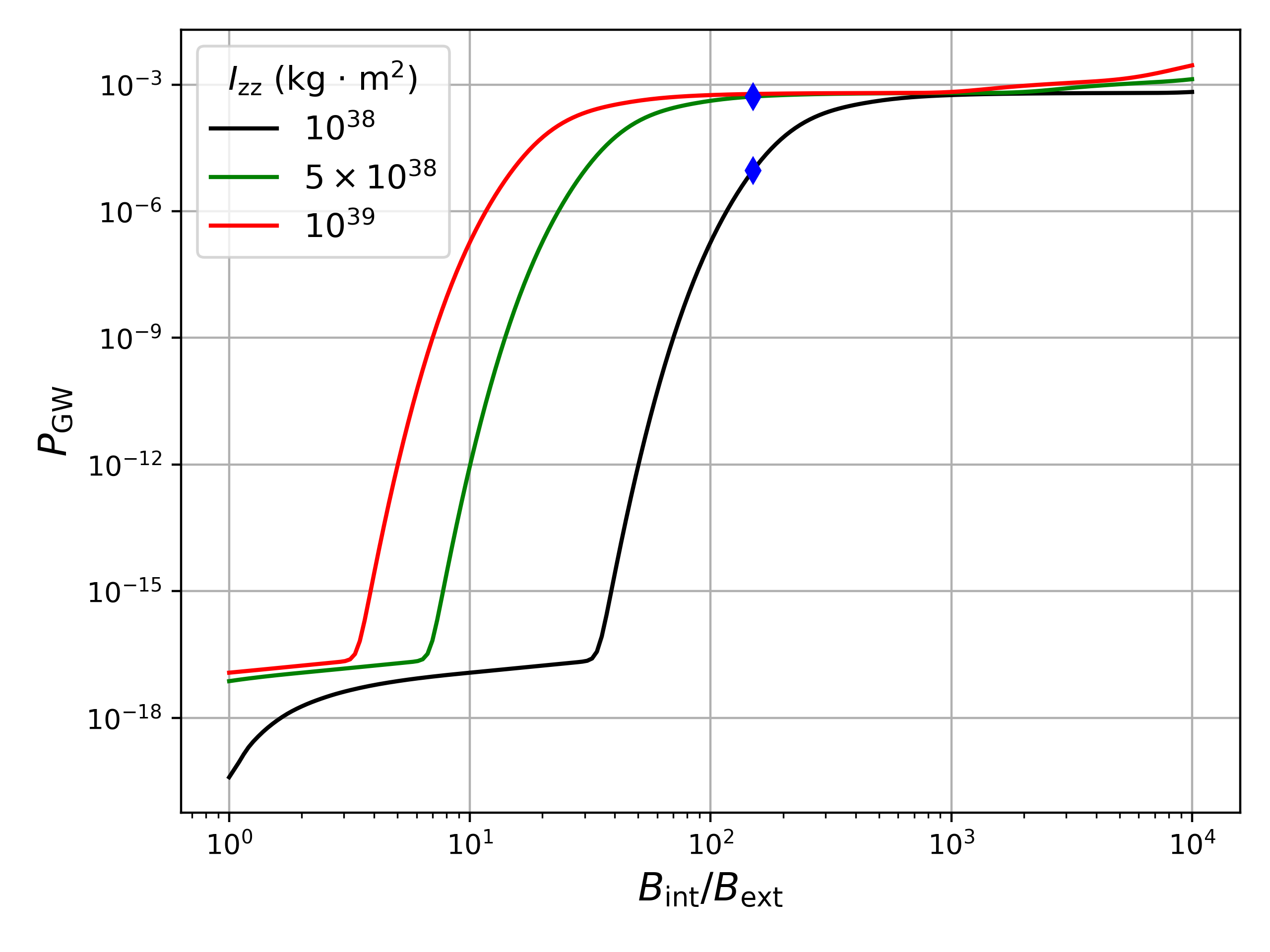
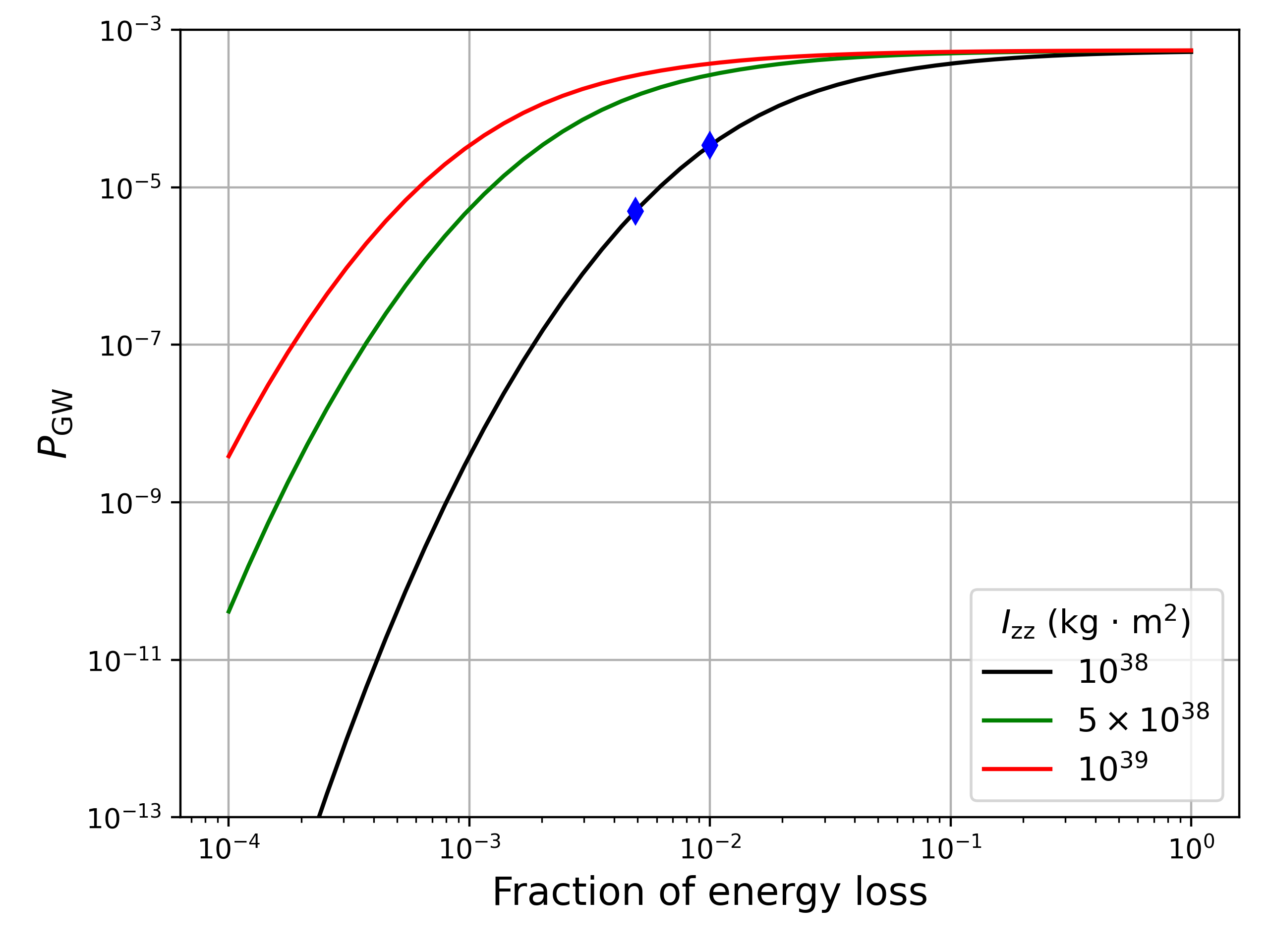
Figure 1: Probability to detect a gravitational-wave signal obtained through Eq. (6), as a function of the internal/external magnetic field ratio (left), and the fraction of rotational energy that we allow to be emitted as gravitational waves (right). The blue diamonds denote the benchmarks that we used to perform concrete analyses with the chosen pulsar luminosity function, see Fig. 2, 9 and 10. $d=8$ kpc.

As an example of what one can do with specific values of $P_{\rm GW}$, we present our results in terms of exclusion regions in the parameter space of a pulsar luminosity function that explains the GeV excess given in Eq. (3) and Eq. (4), in the left- and right-hand panels of Fig. 2, respectively. Here, we consider as a benchmark the “fixed fraction of gravitational-wave energy loss” model, in which 1% of the star’s rotational energy is converted into gravitational waves, given by a blue diamond in Fig. 1. If a pair of luminosity function parameters (e.g. $L_{0}$,$\sigma_{L}$ in Eq. (3), left panel, and $\eta_{\rm med},d_{\gamma}$ in Eq. 4, right panel) results in to too many millisecond pulsars in the Galactic Center, such that at least one of them would have been detected in the O3 Frequency-Hough all-sky search, we can rule out that point in the luminosity function parameter space. The benchmarks of a chosen set of parameters are labeled as blue diamonds in this figure, and are more explored in the App. E, along with exclusion regions showing the permutations of $a_{\gamma},b_{\gamma},$ and $d_{\gamma}$.

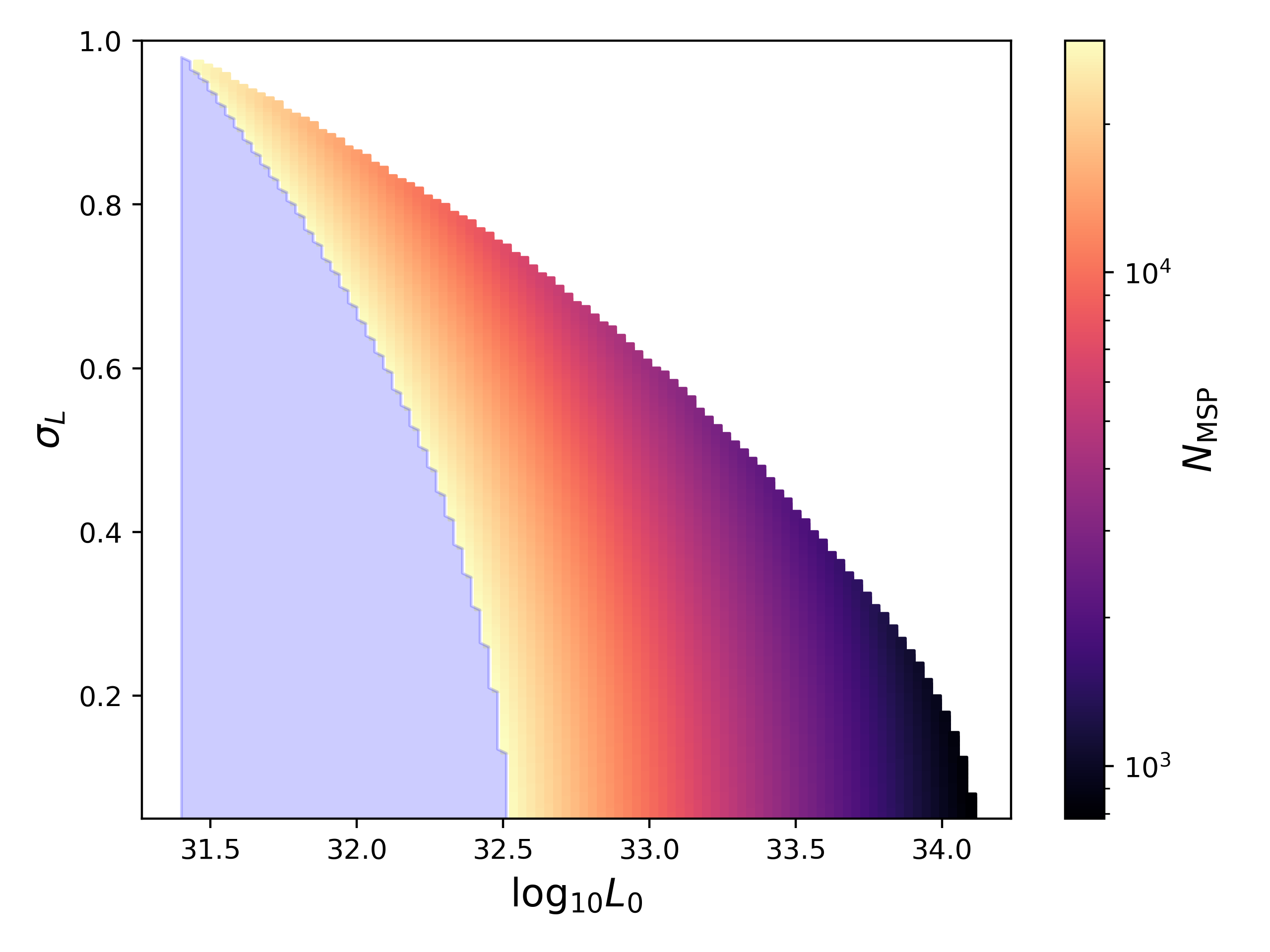
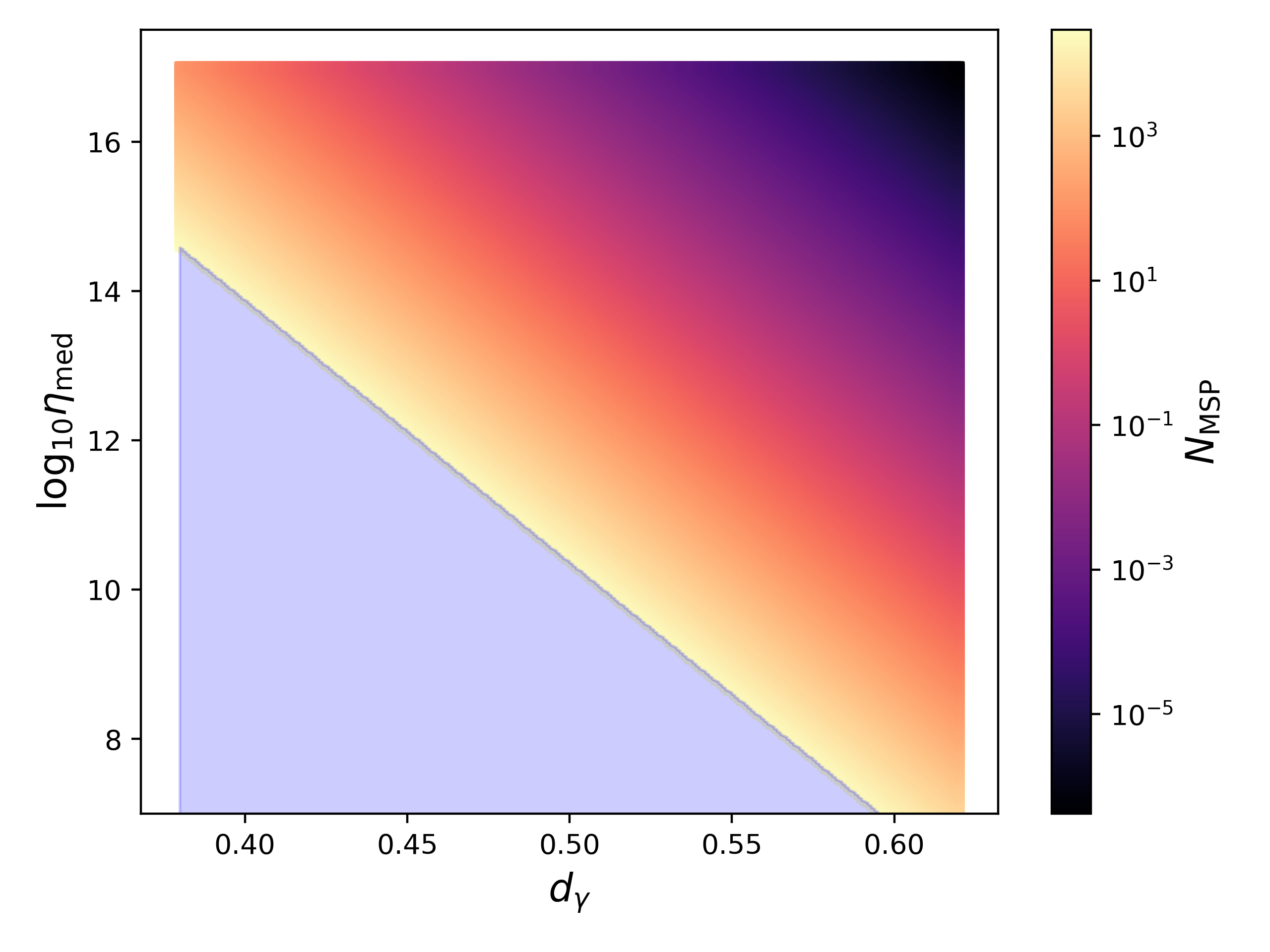
Figure 2: Exclusion regions (light blue) based on the upper limits of the O3 Freuquency-Hough all-sky search for the log-normal (left) and power-law (right) luminosity functions, employing a probability density function for the ellipticity that assumes 1% of the rotational energy loss of the star goes into gravitational waves. We take $d=8$ kpc and $I_{\rm zz}=10^{38}$kg$\cdot$m² in this analysis. The upper-right white region on the left-hand plot has been excluded by Fermi.

V Conclusions

In this work, we have, for the first time, presented gravitational-wave constraints on the millisecond pulsar hypothesis to explain the observed GeV excess by Fermi using LIGO/Virgo/KAGRA data. We used upper limits from the most recent Frequency-Hough all-sky search to calculate the number of detectable millisecond pulsars for various luminosity function parameters, integrating over physically-motivated distributions of rotational frequency and ellipticity. We considered two models for neutron-star deformation, one in which an internal magnetic field sustained the deformation, and another in which we were agnostic to the mechanism of deformation and instead assumed a fixed fraction of rotational energy loss via gravitational waves. For these two models, we computed the probability of detecting a gravitational-wave signal in a search of O3 data, and then excluded portions of the luminosity function parameter space for both models on the basis of null observations for particular parameter choices.

Our exclusion regions depend on (1) the ellipticity distributions we calculate, which themselves are functions of the external magnetic field or the fraction of the rotational energy we assume goes into gravitational waves, (2) the gravitational-wave frequency distribution we use, and (3) the moment of inertia. Furthermore, our results are valid for isolated neutron stars, which comprise about half of all known pulsars (the other half are in binary systems). We show, however, in App. D, that our results would apply to millisecond pulsars in binary systems with certain orbital parameters, given in Fig. 8.

In the future, all-sky gravitational-wave searches will be able to dig deeper into the noise at all frequencies, thus our constraints could be greatly improved. A factor of $5-10$ improvement in the upper limits, expected in third-generation detectors Punturo et al. (2010); Reitze et al. (2019), would allow us to almost completely exclude this luminosity function under the assumptions presented in this work. Furthermore, we plan to devise a template-based method to search for the GeV excess in the Galactic Center by weighting sky pixels by the expected spatial distribution of millisecond pulsars in each one. This approach should improve the sensitivity to millisecond pulsars, and would allow us to incorporate other aspects of millisecond pulsar astrophysics into our work, such as frequency/ellipticity distributions as a function of location. Our future work would also require using finer-resolution sky pixels to explore the inner parsec regions of the Galactic Center, which would add to the computational cost of such gravitational-wave searches and thus needs to be studied.

We also plan to combine the constraints inferred by Fermi and gravitational-wave detectors to probe more portions of the luminosity function parameter space. Furthermore, we could employ correlated frequency/ellipticity probability density functions, e.g. Haskell et al. (2022), that should be more representative of the underlying physics of gravitational-wave emission from millisecond pulsars. Our work therefore represents a major connection between neutron stars, gravitational waves, dark matter, and the Galactic-Center excess.

Appendix A Frequency and Ellipticity distributions

Here we present the frequency and ellipticity distributions derived from the ATNF catalog. The frequency distribution for millisecond pulsars is given in Fig. 3, with a required minimum value of $f_{\rm rot}=60$ Hz. The ellipicity distributions for each deformation model considered – magnetic strain and fixed fraction – are given in Figs. 4 and 5, respectively. These distributions are used as inputs, along with the upper limits from an O3 all-sky search, to determine the number of detectable millisecond pulsars in O3. If we were to use a different frequency distribution as given in Ploeg et al. (2020), we do not expect the exclusion regions to change much, since the integration over the frequency distribution given in Eq. 6 always results in a constant that varies by $\mathcal{O}(1)$. When using the distribution in Fig. 3, we obtain $\int_{\log_{10}f_{\rm min}}^{\log_{10}f_{\rm max}}d\log_{10}fP(\log_{10}f)\sim 0.8$ and for that given in Ploeg et al. (2020), $\sim 1$.

In the magnetic case, we note that larger $B_{\rm int}$ would correspond to bigger ellipticities, which would improve the exclusion regions presented in this work, so even though Fig. 4 quotes a value of $B_{\rm int}=150B_{\rm ext}$, this is a relatively conservative choice with respect to the range of possible ratios (at most $10^{4}$).

For a self-consistency check, gravitational waves would only comprise approximately $\mathcal{O}(0.1\%)$ of the rotational energy of the star, which is calculated using the known $\dot{f}_{\rm rot}$ parameters from the ATNF catalog and comparing that to the gravitational-wave induced spin-down.

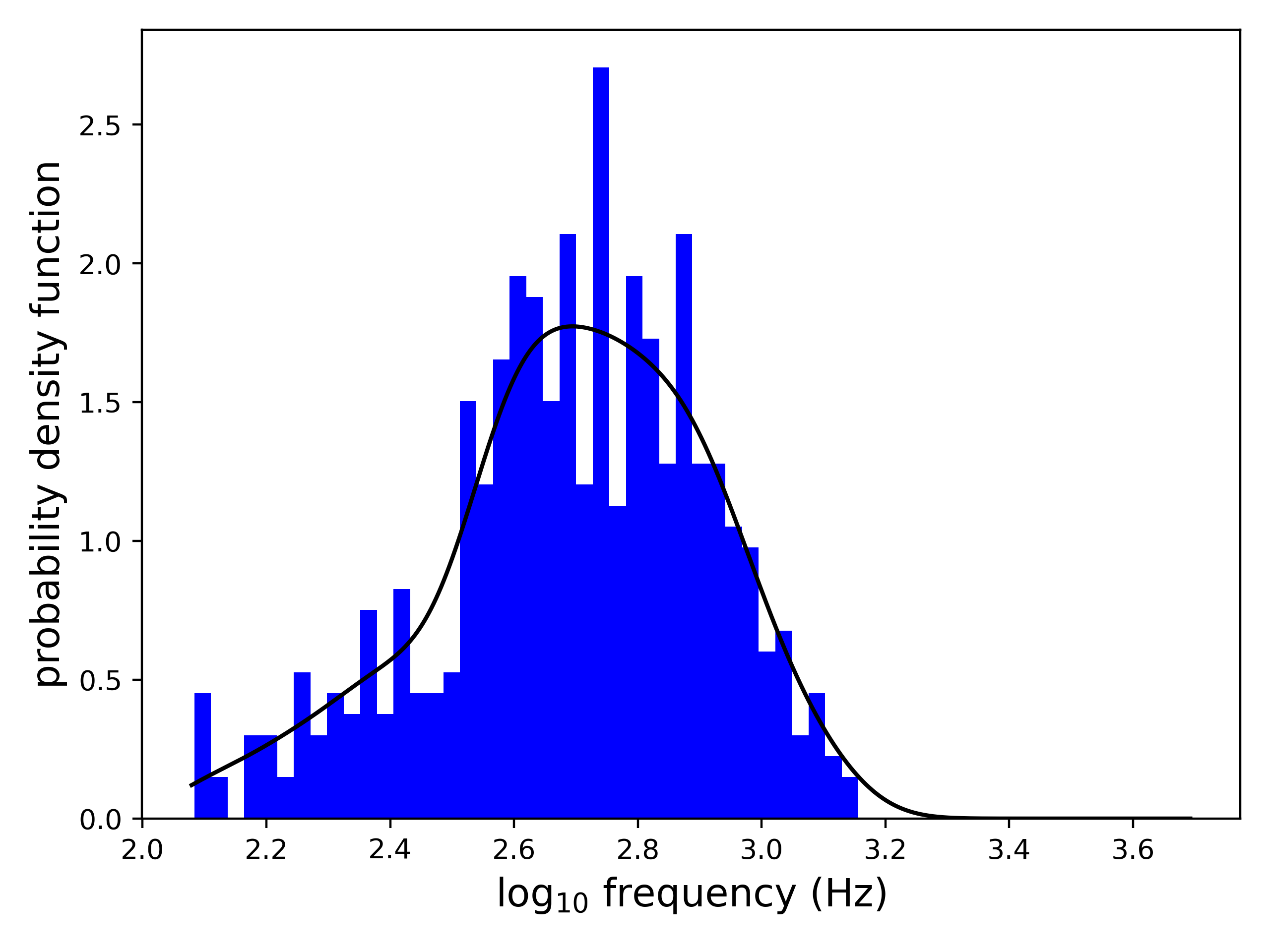
Figure 3: Gravitational-wave frequency probability density function, with a minimum frequency cutoff at $f_{\rm rot}=60$ Hz, ($f_{\rm GW}=120$ Hz) derived from the ATNF catalog Manchester et al. (2005). The black line is a Kernel density estimator fit to the histogram Botev (2023).

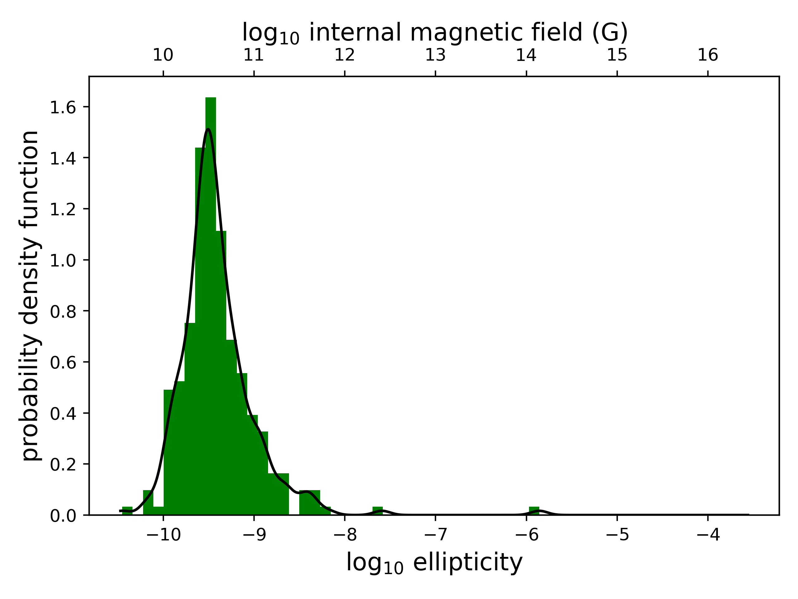
Figure 4: Here we show the ellipticity probability distribution, assuming the deformation of a millisecond pulsar caused by an internal magnetic field. We take the probability distribution of the external magnetic field to be the same as that in the ATNF catalog Manchester et al. (2005), and we use the relation $B_{\rm int}=150B_{\rm ext}$. The black line is a Kernel density estimator fit to the histogram Botev (2023). For reference, the best ellipticity upper limits on some known millisecond pulsars, e.g. J0437–4715, J0711–6830 and J0737–3039A, are $8.3\times 10^{-9},7.2\times 10^{-9}$, and $1.0\times 10^{-6}$ Abbott et al. (2020).

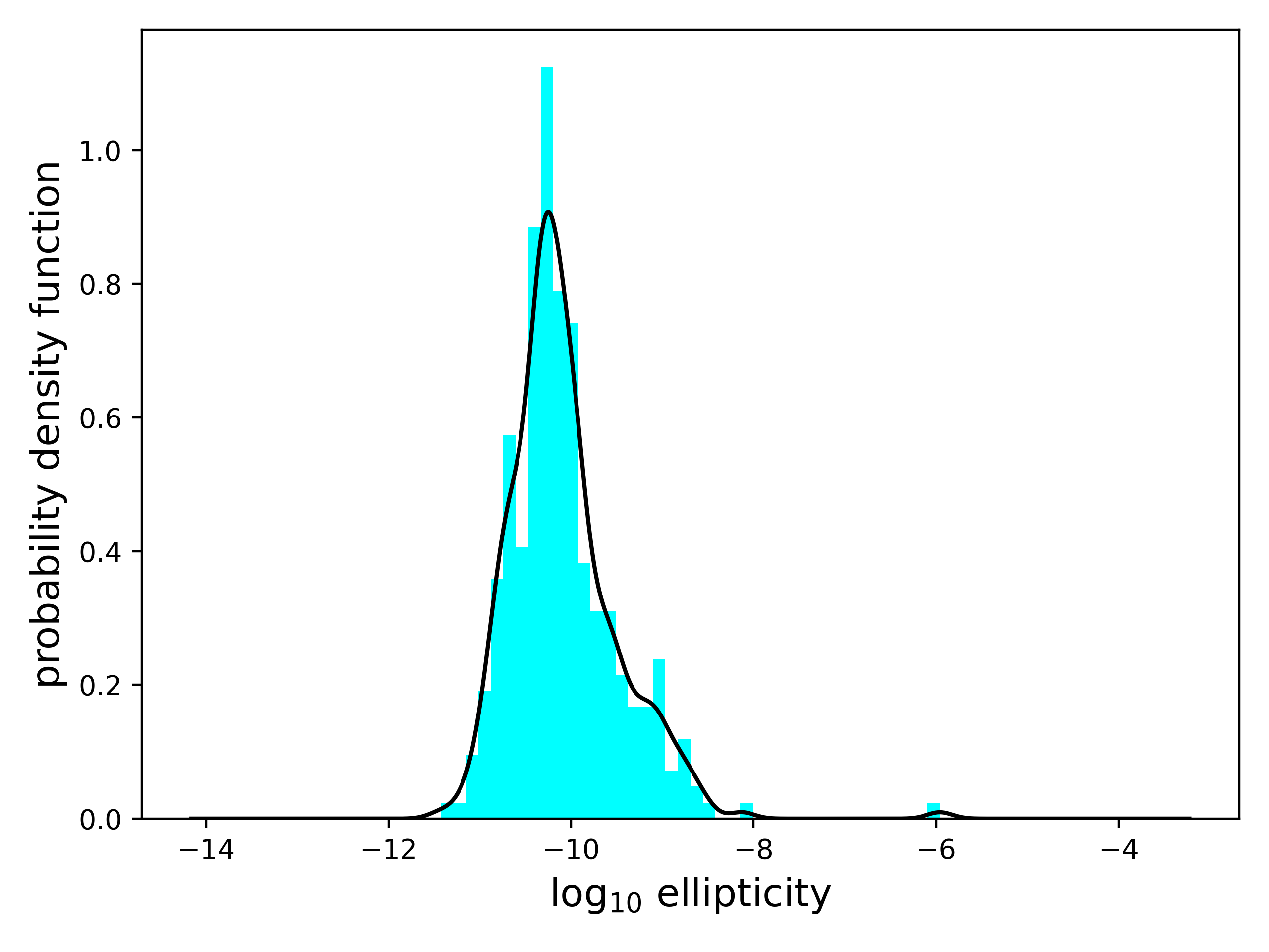
Figure 5: Ellipticity probability density function obtained when assuming that gravitational-wave emission accounts for 1% of the star’s rotational energy loss. $I_{\rm zz}=10^{38}$ kg$\cdot$m². The black line is a Kernel density estimator fit to the histogram Botev (2023).

Appendix B Luminosity Function details

We give more details here about the luminosity functions. The first benchmark luminosity function in Eq. (3) is relatively straightforward. There are two free parameters $L_{0}$ and $\sigma_{L}$. As a comparison with the results in Dinsmore and Slatyer (2022), we further require the following two criteria to be satisfied. First, given the number of millisecond pulsars needed to explain the GeV excess, one should not have too many of them that are above the sensitivity threshold for Fermi 4FGL-DR2. Here we require this to be fewer than 20% of all the 4FGL-DR2 sources, i.e. the number of detectable millisecond pulsars is smaller than 53. Second, we require that the flux of the gamma ray excess at the Galactic Center is not reduced significantly by masking the Fermi 4FGL-DR2 point sources Di Mauro (2021). This demonstrates that the GeV excess should not be dominantly coming from these identified point sources.Thus we require the ratio of the flux emitted by the resolved point sources to be smaller than 20% of the total flux from the Galactic Center.

The second benchmark in Eq. (4) is more general, but it is also quite involved, so let us provide some details. Here $E_{\rm cut}$, $\eta$ and $B$ are assumed to follow the log-normal distribution. The energy emission rate, $\dot{E}$, can be written as $\dot{E}=4\pi^{2}I_{zz}\dot{P}/P^{3}$, where $P$ is the period of a millisecond pulsar. After averaging on the angle between the rotation and magnetic field axes$,\dot{P}$ can further be written as $\dot{P}=5\pi^{2}R_{\rm MSP}^{6}B^{2}/(3c^{3}I_{zz}P)$. The median of $E_{\rm cut}$ is related to $\dot{E}$ as

$$\log_{10}\left(\frac{E_{\rm cut,med}}{{\rm MeV}}\right)=a_{E_{\rm cut}}\log_{10}\left(\frac{\dot{E}}{10^{34.5}\rm erg\ \rm s^{-1}}\right)+b_{E_{\rm cut}}.$$

In Ploeg et al. (2020), all undetermined parameters are obtained by fitting to the GeV excess, see their Table 4 for more details. In our study, we choose their Model A1. Except for $\eta_{\rm med}$ and the power indices {$a_{\gamma}$, $b_{\gamma}$, $d_{\gamma}$}, we take the central values for the rest of the parameters in the luminosity function. We present our results in each pairs of $\eta_{\rm med}$ v.s. one power index, while fixing the other two as their central values.

Following the discussion in Dinsmore and Slatyer (2022), and assuming the luminosity function of millisecond pulsars in the Galactic Center does not have any spatial dependence, the conversion from the total luminosity to the total gamma-ray flux is

$$\frac{F_{\text{GCE}}}{L_{\text{GCE}}} =\frac{1}{4\pi}\left[\int_{\Omega}d\Omega\int_{0}^{\infty}ds\rho_{\text{GCE}}(r)\right]\times$$ (7)

$$\ \ \left[\int_{\Omega}d\Omega\int_{0}^{\infty}s^{2}ds\rho_{\text{GCE}}(r)\right]^{-1}$$

$$=$1.11\text{\times}{10}^{-46}\text{\,}{\mathrm{cm}}^{-2}$.$$ (8)

Here, $s$ and $r$ are the distances from the Earth and Galactic Center to the point of integration, respectively, and $\rho_{\rm GCE}$ is the number density distribution of the millisecond pulsars. We take $\rho_{\rm GCE}$ to be the generalized NFW profile, which is determined by fitting the GeV gamma-ray excess in the Galactic Center,

$$\sqrt{\rho_{\text{GCE}}(r)}\propto(r/r_{s})^{-\gamma}(1+r/r_{s})^{-3+\gamma}.$$ (9)

We choose $\gamma=1.2$ and $r_{s}=20$ kpc Di Mauro (2021); Calore et al. (2015b); Gordon and Macias (2013). We note that this conversion factor is not very sensitive to the millisecond pulsar spatial distribution: it remains almost the same even if all millisecond pulsars are concentrated at the Galactic Center.

The value for the total flux of the Galactic-Center excess can be obtained from Fermi’s measurement. However, the details during the data analysis, such as the fitting procedure and background modeling etc, may lead to a difference of $\mathcal{O}(1)$. A detailed comparison can be found in Dinsmore and Slatyer (2022). In this study, we make a generic choice and set $F=10^{-9}$ erg/cm²/s. Using Eq. (8), we get $L_{\text{GCE}}\approx 10^{37}$ erg/s. Consequently, by integrating over the function, we obtain values of $N_{\rm MSP}$ as a function of various model parameters. This gives us the required number of millisecond pulsars in order to explain the GeV excess observed at the Galactic Center. Later, $N_{\rm MSP}$ will be tested based on the results from the Frequency-Hough all-sky search for continuous waves in O3, see Sec. III.

Appendix C Upper limits from Frequency-Hough all-sky search and the conversion factor to a directed search

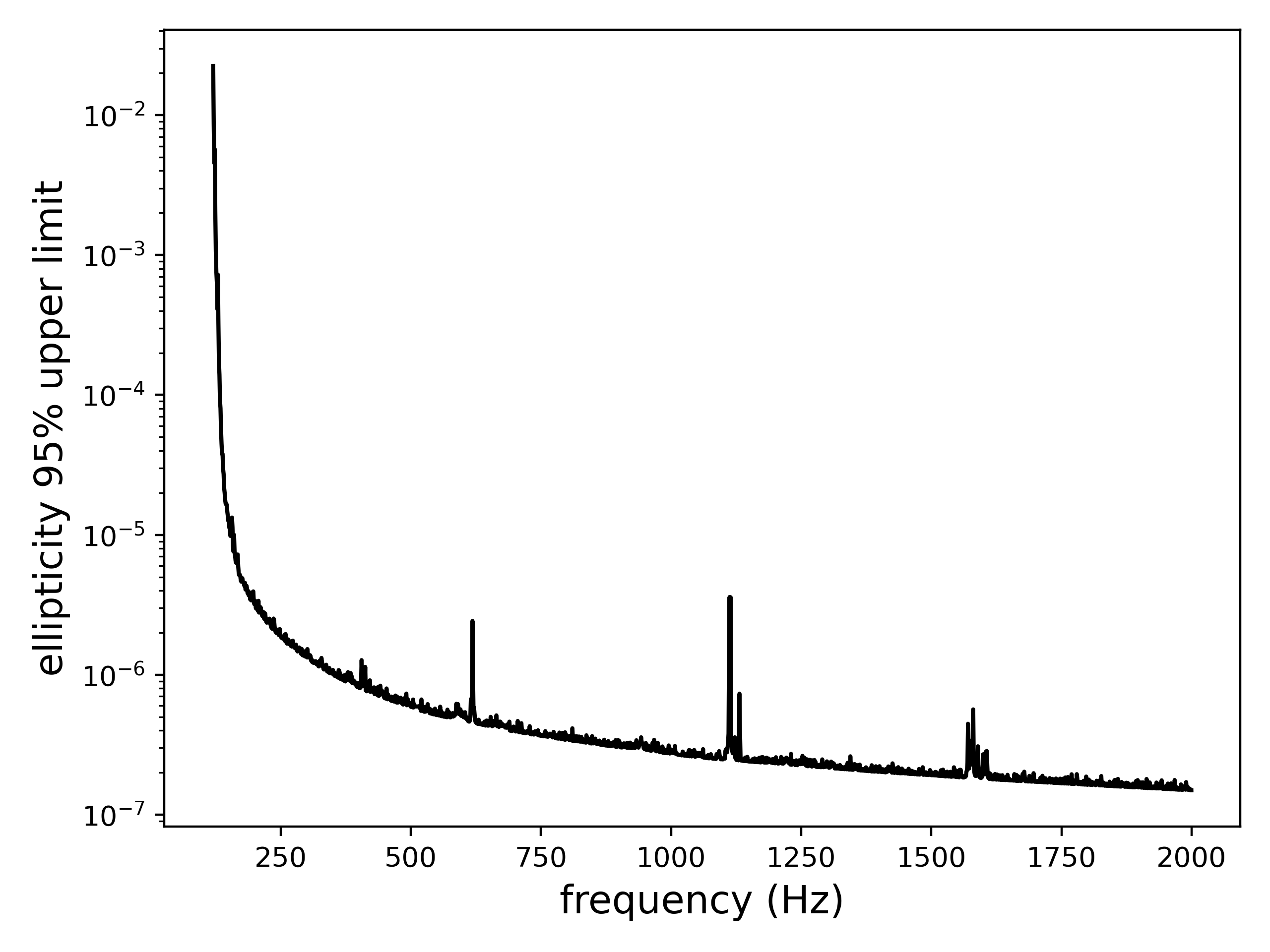
Figure 6: Upper limits on ellipticity as a function of gravitational-wave frequency from the Frequency-Hough all-sky search in the third observing run of LIGO/Virgo/KAGRA. One sets $d=8$ kpc, $I_{\rm zz}=10^{38}$ kg$\cdot$m², to generate these limits.

We provide here the Frequency-Hough all-sky upper limits on ellipticity from Abbott et al. (2022a), in Fig. 6, averaged over sky location. These limits, initially derived in terms of strain as a function of frequency, are translated to limits on the ellipticity using Eq. (1).

Furthermore, in order to calculate the conversation factor needed to “specialize” the sky-averaged limits to the pixels surrounding the Galactic Center, we start with the following (abridged) formula used in Abbott et al. (2022a) that relates the geometric factor $\mathcal{S}$ to how a monochromatic gravitational wave couples to the detector:

$$\mathcal{S}^{2}=\left(A_{+}F_{+}+A_{\times}F_{\times}\right)^{2}.$$ (10)

$F_{+}$ and $F_{\times}$ are the time-dependent detector beam pattern functions that convey directional and temporal sensitivity to all sky locations, which are:

$$F_{+}(t)=a(t)\cos 2\psi+b(t)\sin 2\psi$$ (11)

$$F_{\times}(t)=b(t)\cos 2\psi-a(t)\sin 2\psi.$$

$t$ is time, $a(t)$ and $~{}b(t)$ can be found in Jaranowski et al. (1998) and depend on the detector and source location, and $\psi$ is the gravitational-wave polarization angle. The terms $A_{+}$ and $~{}A_{\times}$ are:

$$A_{+}=\frac{1+\cos^{2}\iota}{2}$$ (12)

$$A_{\times}=\cos\iota,$$

where $\iota$ is the inclination angle between the Earth and the neutron star. In Abbott et al. (2022a), the upper limits are computed by taking the average over all the source parameters, which gives an overall factor of:

$$\mathcal{S}^{2}_{\alpha,~{}\delta,~{}\psi,~{}\iota}=<\mathcal{F}^{2}>_{\alpha,\delta,\psi,\iota}\simeq\frac{4}{25},$$ (13)

approximately independent of which detector that is considered. $\alpha$, $\delta$ and $\psi$ are the right ascension, and declination, and polarization angle, respectively, of a source.

Here, we only need to average over $\psi$, $\cos\iota$, and $t$ to obtain a sky-dependent factor:

$$\mathcal{S}^{2}_{~{}\psi,~{}\iota}=<F^{2}_{+}>_{t,\psi}<A^{2}_{+}>_{\iota}+<F^{2}_{\times}>_{t,\psi}<A^{2}_{\times}>_{\iota}$$ (14)

When we take the ratio of Eq. (13) to Eq. (14), we obtain a factor by which we multiply the upper limit in Abbott et al. (2022a) at a fixed frequency, to obtain a sky-dependent upper limit:

$$\mathcal{C}(\alpha,\delta)=\sqrt{\frac{\mathcal{S}^{2}_{\alpha,~{}\delta,~{}\psi,~{}\iota}}{\mathcal{S}^{2}_{~{}\psi,~{}\iota}}}.$$ (15)

In Fig. 7, we produce a skymap at $f=2000$ Hz that shows $\mathcal{C}(\alpha,\delta)$. We can see that, for different pixels, $\mathcal{C}(\alpha,\delta)$ changes by no more than a few percent in either direction from 1, indicating that the upper limits used in one pixel are reflective of considering a larger number of sky pixels in the Galactic Center. Note that the skymap looks different at each frequency: the number of sky points scales with the square of the gravitational-wave frequency, since the criterium to grid the sky requires that when moving from one point to another, the modulation induced by the Doppler effect is confined to one frequency bin Astone et al. (2014). However, the percent change in the upper limits as a function of sky location remains about the same, regardless of the frequency.

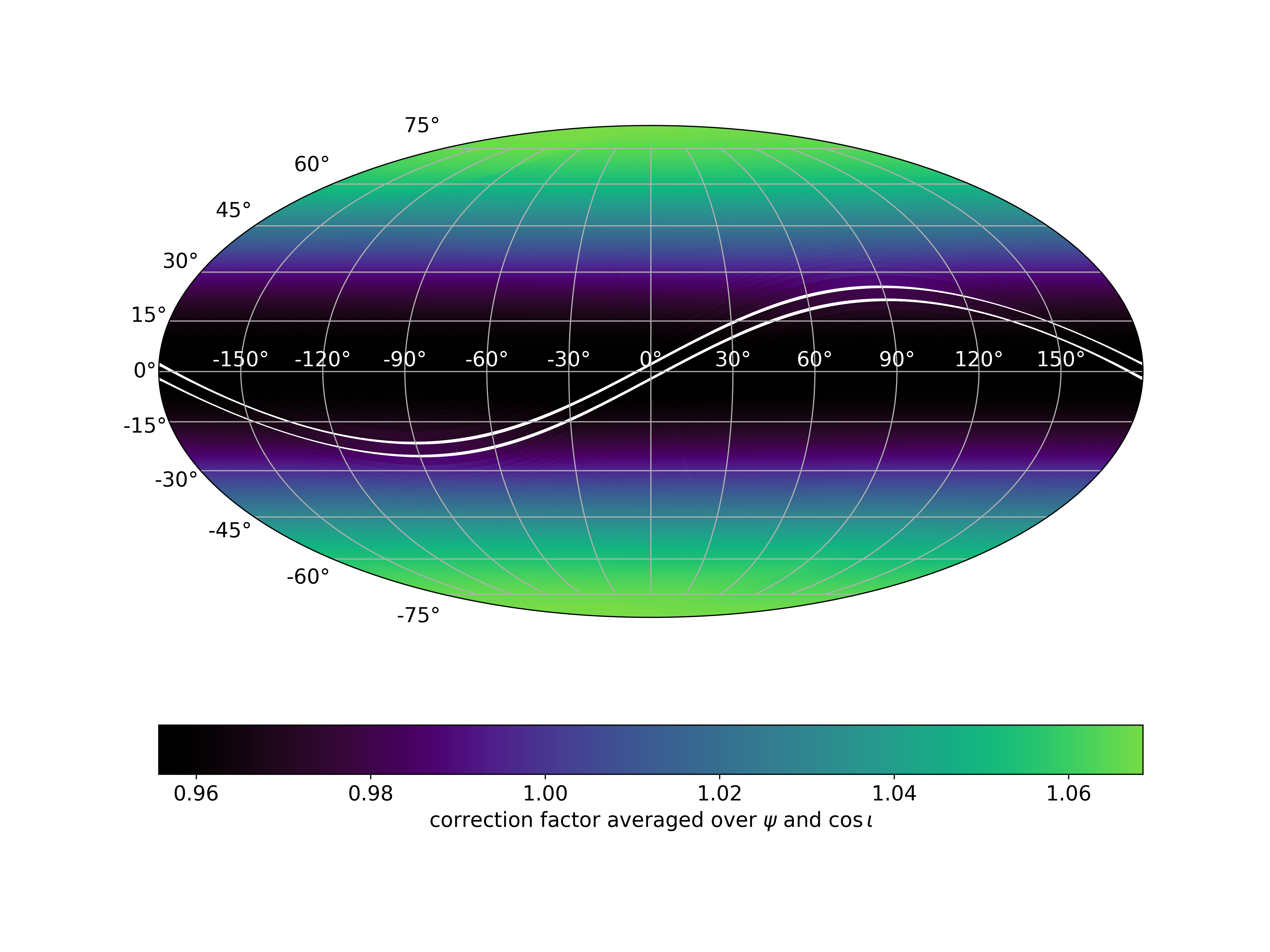
Figure 7: Here we show the factor by which upper limits from the Frequency-Hough all-sky search need to be multiplied to obtain sky-dependent ellipticity upper limits at 2000 Hz. Note that the sky grid is a function of frequency Astone et al. (2014).

Appendix D Millisecond pulsars in binary systems

The results presented here are valid if millisecond pulsars are isolated, but one expects that $O(1)$ fraction of them exist in binary systems Tauris et al. (2017). We thus compute the orbital parameters of binary systems to which our results could apply by requiring that the Doppler modulation induced by the orbital motion of the system is contained within one frequency bin, and neglecting orbital eccentricity Abbott et al. (2019):

$$a_{p}\leq 0.076\left(\frac{P}{1\text{ day}}\right)\left(\frac{f}{100\text{ Hz}}\right)^{-1}\left(\frac{T_{\text{FFT}}}{1800\text{ s}}\right)^{-1}\text{ l$\cdot$s}.$$ (16)

Here, $a_{p}$ is the semi-major axis with units light-seconds l$\cdot$s , $P$ is the orbital period, and $T_{\text{FFT}}$ is the Fast Fourier Transform length used in the search, which is also a function of frequency. Fig. 8 shows the orbital parameter space $a_{p}$ and $P$ to which we are sensitive, as a function of gravitational-wave frequency. Our results are thus valid for millisecond pulsars in binary systems whose orbital parameters lie within these ranges. We note, however, that about half of known millisecond pulsars are found in binary systems, and of those, only a small fraction of known millisecond pulsars lie within this parameter space.

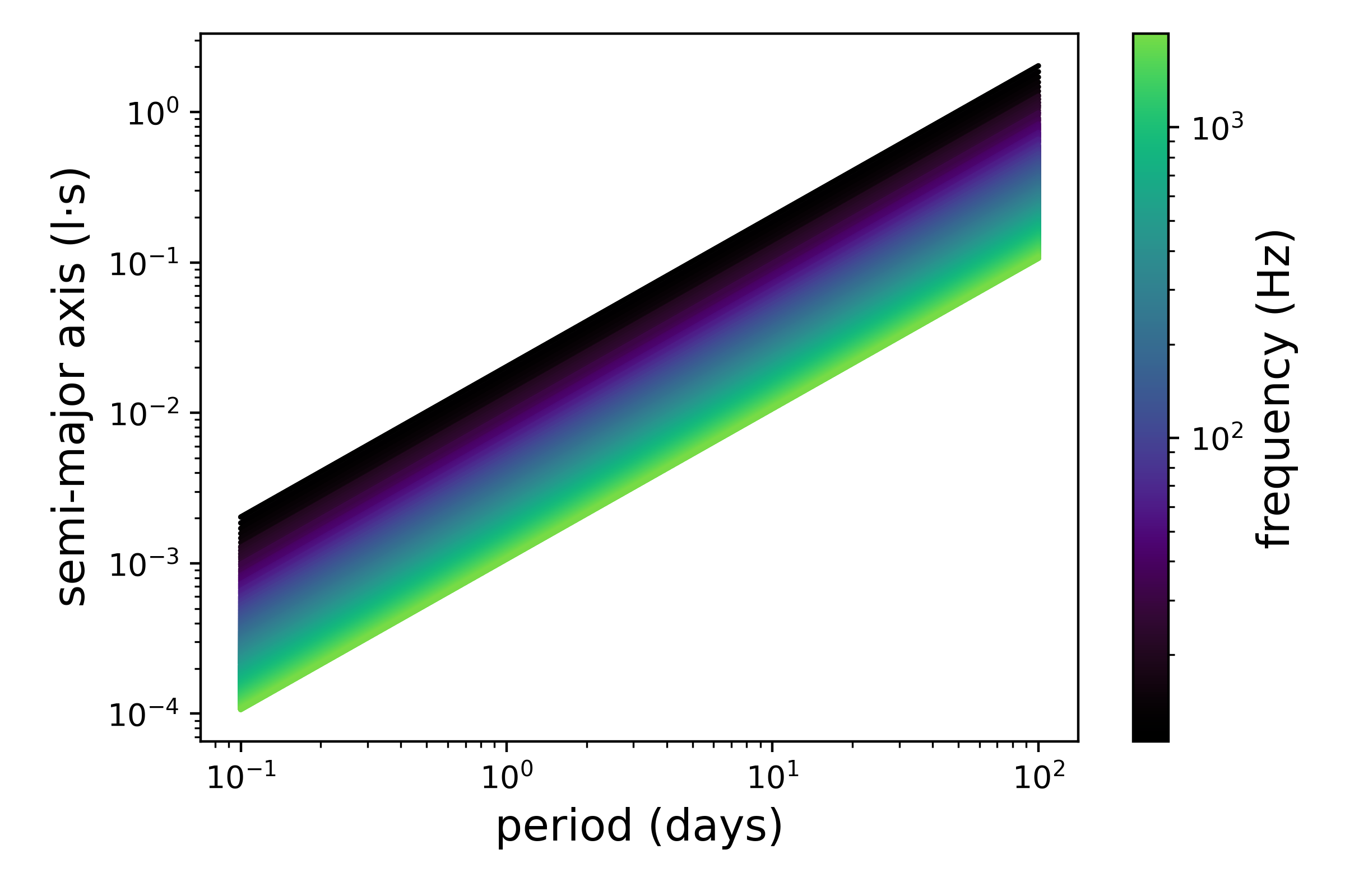
Figure 8: Parameter space of millisecond pulsars in binary systems to which our constraints would apply. Note that only a small fraction of the orbital parameters of known millisecond pulsars in binary systems lie within this range.

Appendix E How exclusion regions vary based on $I_{\rm zz}$, $d$ and fraction of energy loss

We present in Fig. 9 exclusion regions (light blue) in the $L_{0}$/$\sigma_{L}$ parameter space if the neutron-star ellipticity is sustained by an internal magnetic field, as explained in Sec. II.2, and at least one millisecond pulsar would have been detected in the O3 all-sky search in the Galactic Center. The results are obtained with two values of the moment of inertia, $I_{\rm zz}=10^{38}$ kg$\cdot$m² (left) and $I_{\rm zz}=5\times 10^{38}$ kg$\cdot$m² (right), which correspond to different equations of states of millisecond pulsars. Here, we see that the constraint becomes more stringent if millisecond pulsars have a higher moment of inertia, given fixed $B_{\rm int}$. This is because the ellipticity upper limits from the all-sky search, shown in App. C, would be lowered by a factor of 5 across all frequencies. Consequently, it leads to a larger probability for millisecond pulsars to be excluded from existing.

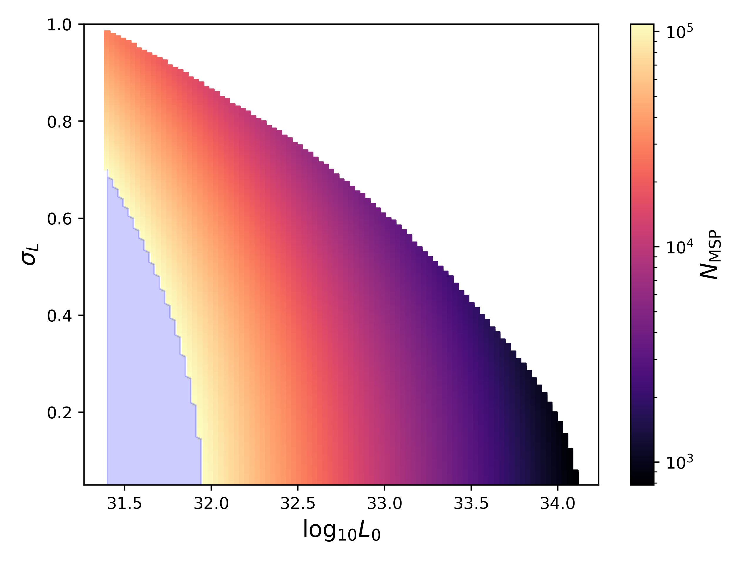
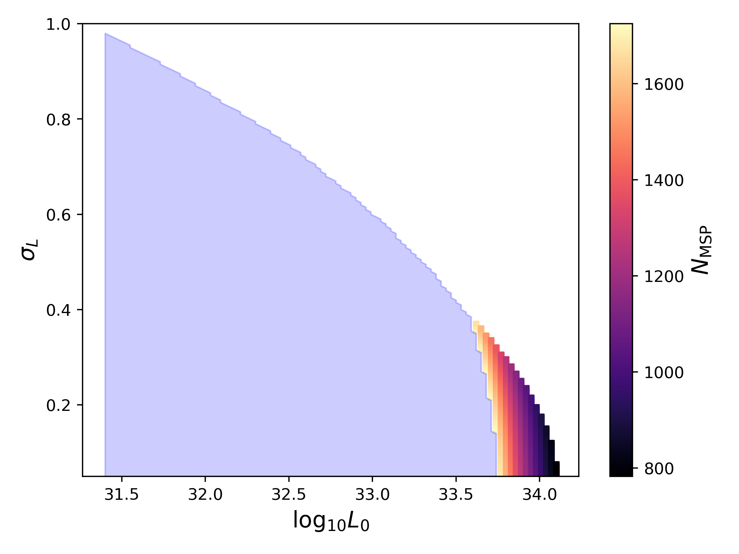
Figure 9: Exclusion regions (light blue) based on the upper limits of the O3 Frequency-Hough all-sky search using the log-normal luminosity function (Eq. 3). In these regions, the number of detectable millisecond pulsars with LIGO/Virgo data exceeds one. We take $B_{\rm int}=150B_{\rm ext}$; $d=8$ kpc, and left: $I_{\rm zz}=10^{38}$kg$\cdot$m²; right: $I_{\rm zz}=5\times 10^{38}$kg$\cdot$m². With these parameters, less than $\mathcal{O}(1\%)$ of the total rotational energy loss of the star is through gravitational-wave radiations. The upper-right white regions on both plots have been excluded by Fermi.

In Fig. 10, we show similar constraints when allowing a fixed fraction of rotational energy to be converted into gravitational waves. The plot corresponds to the fraction taken to be 0.25% at a fixed moment of inertia. If gravitational waves take more rotational energy from the star, we are able to exclude larger portions of the $L_{0}$/$\sigma_{L}$ parameter space.

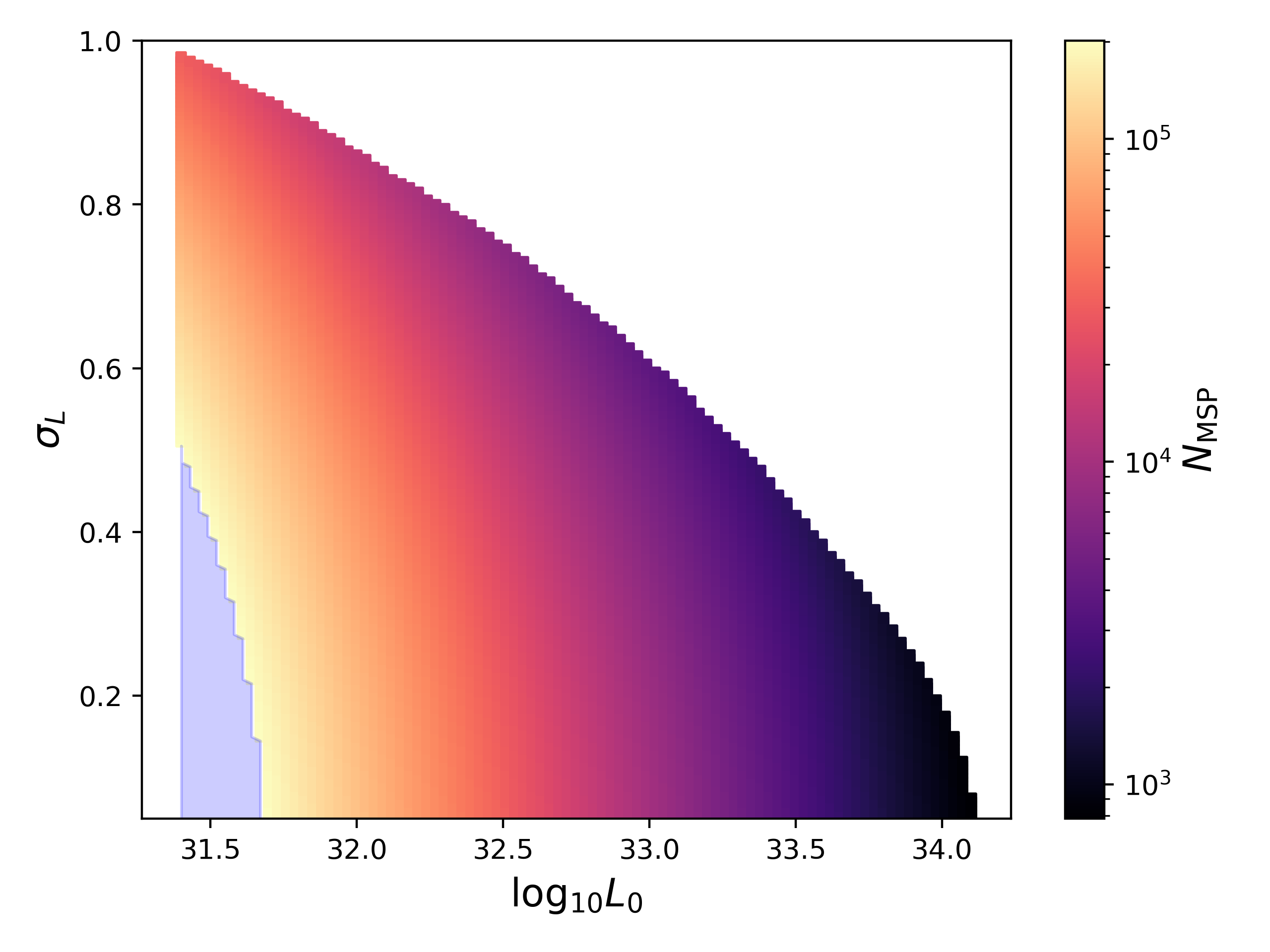
Figure 10: Exclusion regions (light blue) based on the upper limits of the O3 Freuquency-Hough all-sky search using the log-normal luminosity function (Eq. 3), employing a probability density function for the ellipticity that assumes 0.5% of the rotational energy loss of the star goes into gravitational waves. We take $d=8$ kpc and $I_{\rm zz}=10^{38}$kg$\cdot$m² in this analysis. The upper-right white region has been excluded by Fermi.

We also determine how sensitive our exclusion regions are to distance reach, picking 6 or 10 kpc to contrast with 8 kpc used throughout the paper. Millisecond pulsars could in fact be closer than 8 kpc to us if they live in the “boxy bulge” (a part of the Galactic bar) Macias et al. (2018); Bartels et al. (2018) and thus our constraints would be more stringent on them there. We show in Fig. 11 exclusion regions for 6 kpc (left) and 10 kpc (right) systems.

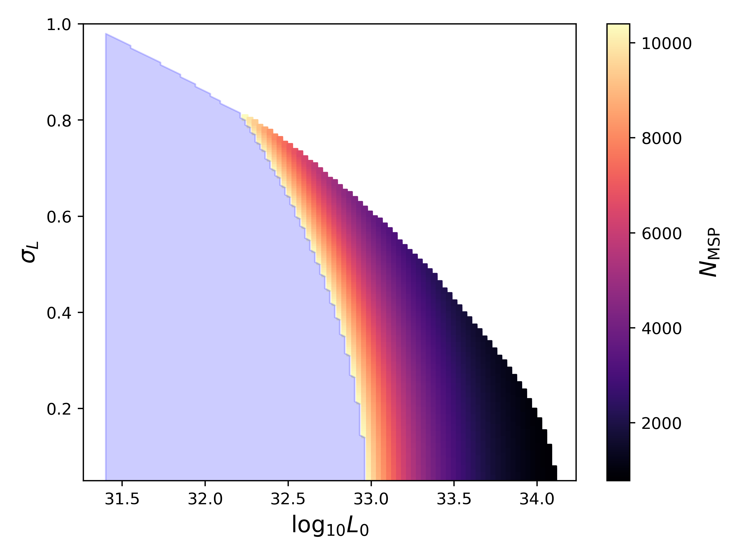
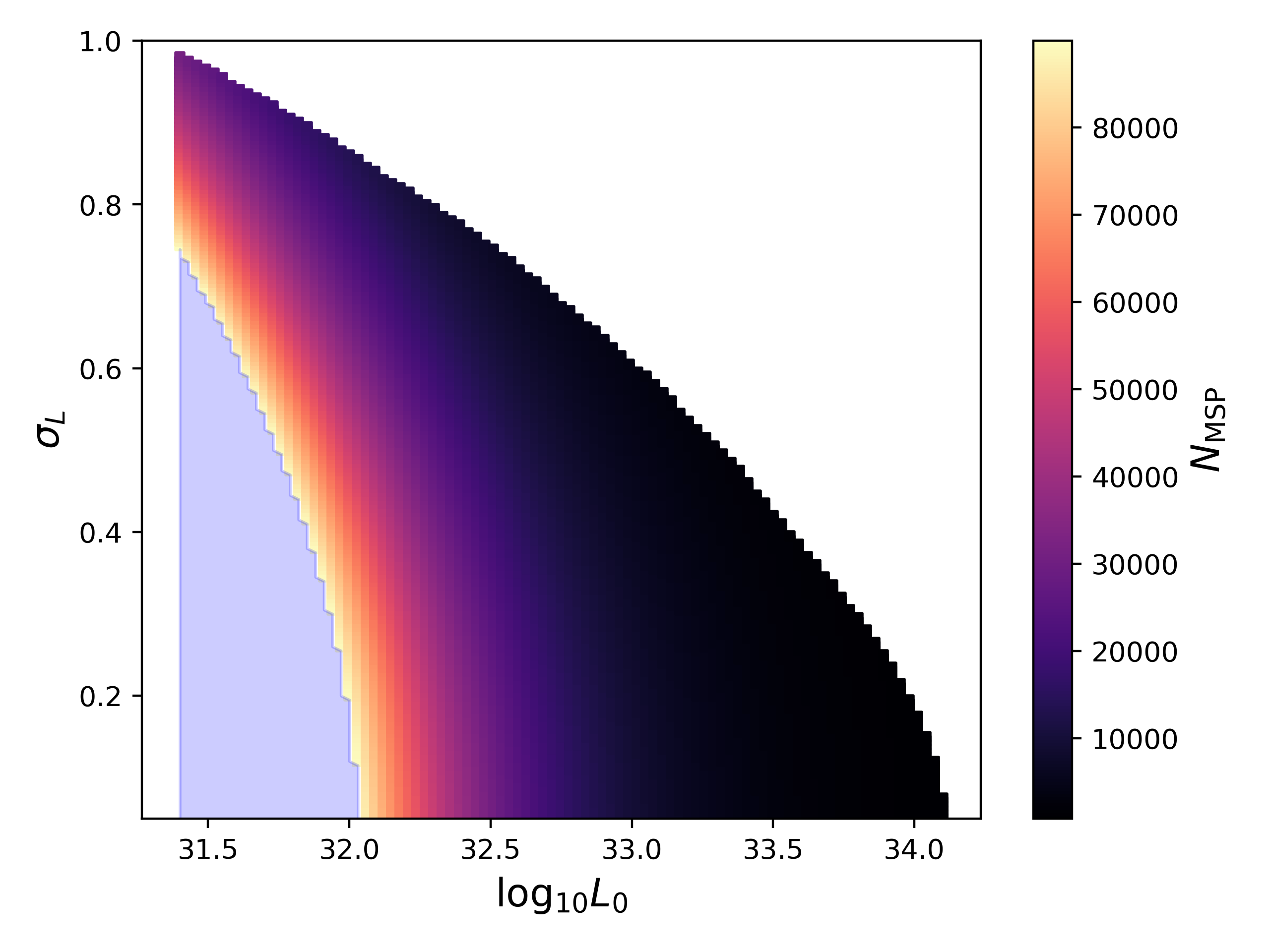
Figure 11: Exclusion regions (light blue) based on the upper limits of the O3 Frequency-Hough all-sky search using the log-normal luminosity function (Eq. 3). In these regions, the number of detectable millisecond pulsars with LIGO/Virgo data exceeds one. We take $I_{\rm zz}=10^{38}$kg$\cdot$m² and $d=6$ kpc (left) and $d=8$ kpc (right), and allow only 1% of rotational energy to be converted to gravitational waves.

Finally, we also provide exclusion plots for two other parameterizations of the power-law luminosity function model (Eq. 4 in Fig. 12). We can see that portions of the parameter space for these two choices of power-law luminosity function can also be excluded by continuous-wave upper limits.

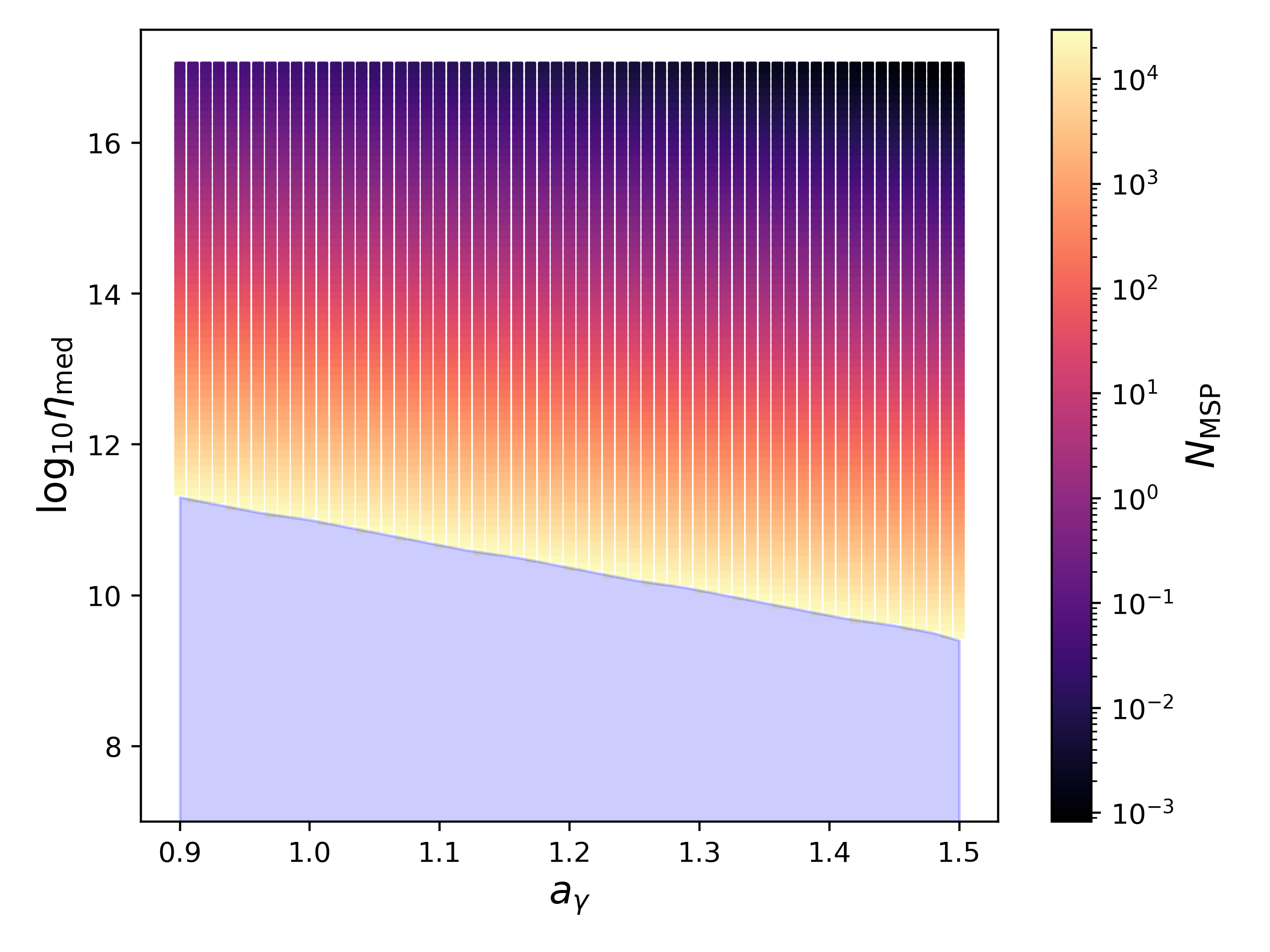
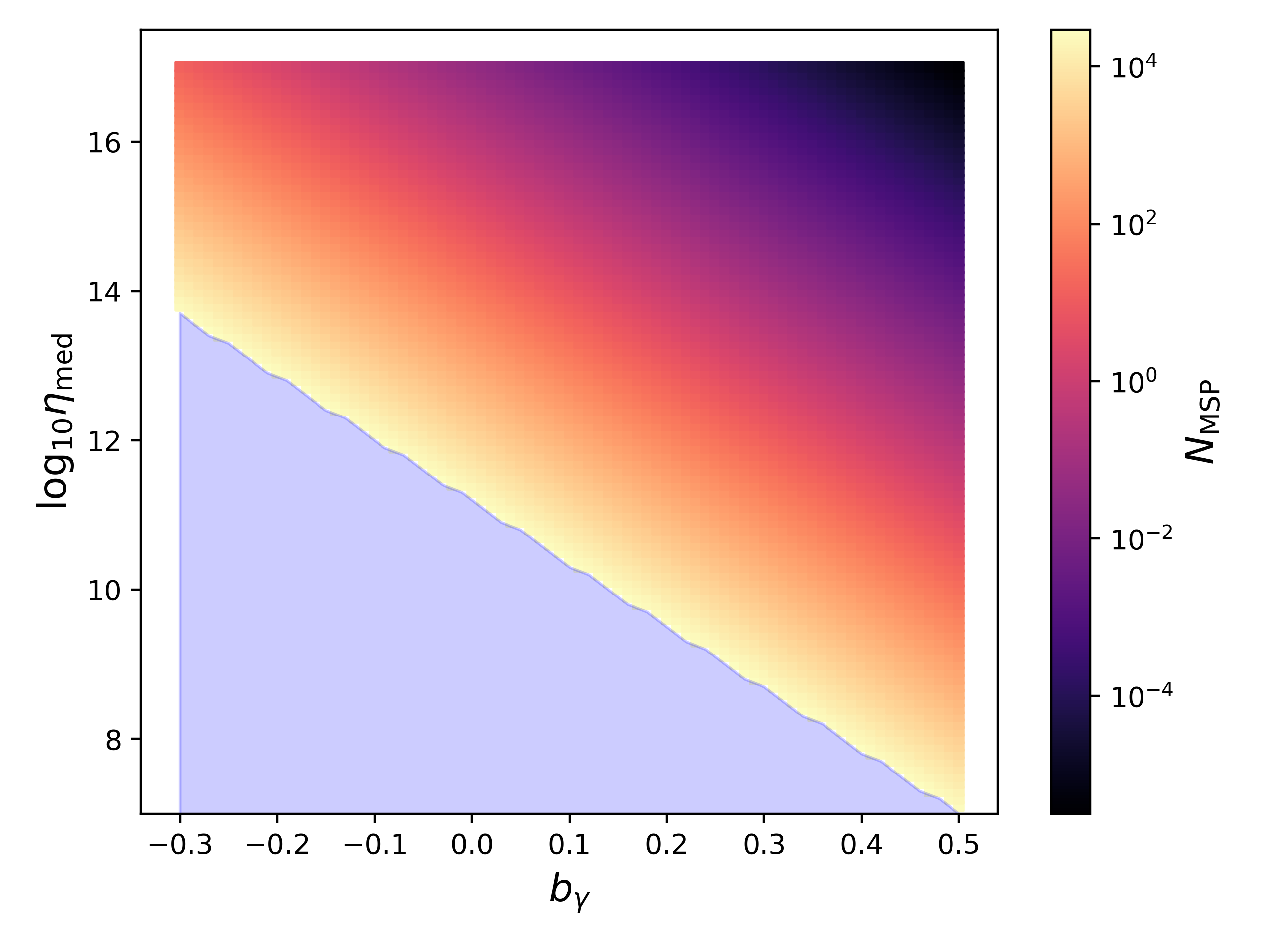
Figure 12: Exclusion regions (light blue) based on the upper limits of the O3 Frequency-Hough all-sky search using the power-law luminosity function (Eq. 4). In these regions, the number of detectable millisecond pulsars with LIGO/Virgo data exceeds one. We take $I_{\rm zz}=10^{38}$kg$\cdot$m², $d=8$ kpc, and allow only 1% of rotational energy to be converted to gravitational waves. The range of $N_{\rm MSP}$ is taken to include the values within the error bars of Ploeg et al. (2020).

References

- Goodenough and Hooper (2009) L. Goodenough and D. Hooper, (2009), arXiv:0910.2998 [hep-ph] .
- Hooper and Goodenough (2011) D. Hooper and L. Goodenough, Phys. Lett. B 697, 412 (2011), arXiv:1010.2752 [hep-ph] .
- Hooper and Linden (2011) D. Hooper and T. Linden, Phys. Rev. D 84, 123005 (2011), arXiv:1110.0006 [astro-ph.HE] .
- Gordon and Macias (2013) C. Gordon and O. Macias, Phys. Rev. D 88, 083521 (2013), [Erratum: Phys.Rev.D 89, 049901 (2014)], arXiv:1306.5725 [astro-ph.HE] .
- Daylan et al. (2016) T. Daylan, D. P. Finkbeiner, D. Hooper, T. Linden, S. K. N. Portillo, N. L. Rodd, and T. R. Slatyer, Phys. Dark Univ. 12, 1 (2016), arXiv:1402.6703 [astro-ph.HE] .
- Calore et al. (2015a) F. Calore, I. Cholis, C. McCabe, and C. Weniger, Phys. Rev. D 91, 063003 (2015a), arXiv:1411.4647 [hep-ph] .
- Abazajian et al. (2014) K. N. Abazajian, N. Canac, S. Horiuchi, and M. Kaplinghat, Phys. Rev. D 90, 023526 (2014), arXiv:1402.4090 [astro-ph.HE] .
- Petrović et al. (2014) J. Petrović, P. D. Serpico, and G. Zaharijaš, JCAP 10, 052 (2014), arXiv:1405.7928 [astro-ph.HE] .
- Carlson and Profumo (2014) E. Carlson and S. Profumo, Phys. Rev. D 90, 023015 (2014), arXiv:1405.7685 [astro-ph.HE] .
- Cholis et al. (2015a) I. Cholis, C. Evoli, F. Calore, T. Linden, C. Weniger, and D. Hooper, JCAP 12, 005 (2015a), arXiv:1506.05119 [astro-ph.HE] .
- Abazajian (2011) K. N. Abazajian, JCAP 03, 010 (2011), arXiv:1011.4275 [astro-ph.HE] .
- Calore et al. (2015b) F. Calore, I. Cholis, and C. Weniger, JCAP 03, 038 (2015b), arXiv:1409.0042 [astro-ph.CO] .
- Yuan and Zhang (2014) Q. Yuan and B. Zhang, JHEAp 3-4, 1 (2014), arXiv:1404.2318 [astro-ph.HE] .
- Petrović et al. (2015) J. Petrović, P. D. Serpico, and G. Zaharijas, JCAP 02, 023 (2015), arXiv:1411.2980 [astro-ph.HE] .
- Ye and Fragione (2022) C. S. Ye and G. Fragione, Astrophys. J. 940, 162 (2022), arXiv:2207.03504 [astro-ph.HE] .
- Macias et al. (2018) O. Macias, C. Gordon, R. M. Crocker, B. Coleman, D. Paterson, S. Horiuchi, and M. Pohl, Nature Astron. 2, 387 (2018), arXiv:1611.06644 [astro-ph.HE] .
- Bartels et al. (2018) R. Bartels, E. Storm, C. Weniger, and F. Calore, Nature Astron. 2, 819 (2018), arXiv:1711.04778 [astro-ph.HE] .
- Macias et al. (2019) O. Macias, S. Horiuchi, M. Kaplinghat, C. Gordon, R. M. Crocker, and D. M. Nataf, JCAP 09, 042 (2019), arXiv:1901.03822 [astro-ph.HE] .
- Pohl et al. (2022) M. Pohl, O. Macias, P. Coleman, and C. Gordon, Astrophys. J. 929, 136 (2022), arXiv:2203.11626 [astro-ph.HE] .
- Di Mauro (2021) M. Di Mauro, Phys. Rev. D 103, 063029 (2021), arXiv:2101.04694 [astro-ph.HE] .
- Cholis et al. (2022) I. Cholis, Y.-M. Zhong, S. D. McDermott, and J. P. Surdutovich, Phys. Rev. D 105, 103023 (2022), arXiv:2112.09706 [astro-ph.HE] .
- Lee et al. (2015) S. K. Lee, M. Lisanti, and B. R. Safdi, JCAP 05, 056 (2015), arXiv:1412.6099 [astro-ph.CO] .
- Lee et al. (2016) S. K. Lee, M. Lisanti, B. R. Safdi, T. R. Slatyer, and W. Xue, Phys. Rev. Lett. 116, 051103 (2016), arXiv:1506.05124 [astro-ph.HE] .
- Buschmann et al. (2020) M. Buschmann, N. L. Rodd, B. R. Safdi, L. J. Chang, S. Mishra-Sharma, M. Lisanti, and O. Macias, Phys. Rev. D 102, 023023 (2020), arXiv:2002.12373 [astro-ph.HE] .
- Leane and Slatyer (2019) R. K. Leane and T. R. Slatyer, Phys. Rev. Lett. 123, 241101 (2019), arXiv:1904.08430 [astro-ph.HE] .
- Leane and Slatyer (2020a) R. K. Leane and T. R. Slatyer, Phys. Rev. Lett. 125, 121105 (2020a), arXiv:2002.12370 [astro-ph.HE] .
- Leane and Slatyer (2020b) R. K. Leane and T. R. Slatyer, Phys. Rev. D 102, 063019 (2020b), arXiv:2002.12371 [astro-ph.HE] .
- Hooper et al. (2013) D. Hooper, I. Cholis, T. Linden, J. Siegal-Gaskins, and T. Slatyer, Phys. Rev. D 88, 083009 (2013), arXiv:1305.0830 [astro-ph.HE] .
- Hooper and Linden (2016) D. Hooper and T. Linden, JCAP 08, 018 (2016), arXiv:1606.09250 [astro-ph.HE] .
- Ploeg et al. (2020) H. Ploeg, C. Gordon, R. Crocker, and O. Macias, JCAP 12, 035 (2020), [Erratum: JCAP 07, E01 (2021)], arXiv:2008.10821 [astro-ph.HE] .
- List et al. (2021) F. List, N. L. Rodd, and G. F. Lewis, Phys. Rev. D 104, 123022 (2021), arXiv:2107.09070 [astro-ph.HE] .
- Gautam et al. (2022) A. Gautam, R. M. Crocker, L. Ferrario, A. J. Ruiter, H. Ploeg, C. Gordon, and O. Macias, Nature Astron. 6, 703 (2022), arXiv:2106.00222 [astro-ph.HE] .
- Cholis et al. (2015b) I. Cholis, D. Hooper, and T. Linden, JCAP 06, 043 (2015b), arXiv:1407.5625 [astro-ph.HE] .
- Haggard et al. (2017) D. Haggard, C. Heinke, D. Hooper, and T. Linden, JCAP 05, 056 (2017), arXiv:1701.02726 [astro-ph.HE] .
- Berteaud et al. (2021) J. Berteaud, F. Calore, M. Clavel, P. D. Serpico, G. Dubus, and P.-O. Petrucci, Phys. Rev. D 104, 043007 (2021), arXiv:2012.03580 [astro-ph.HE] .
- Macias et al. (2021) O. Macias, H. van Leijen, D. Song, S. Ando, S. Horiuchi, and R. M. Crocker, Mon. Not. Roy. Astron. Soc. 506, 1741 (2021), arXiv:2102.05648 [astro-ph.HE] .
- Calore et al. (2016) F. Calore, M. Di Mauro, F. Donato, J. W. T. Hessels, and C. Weniger, Astrophys. J. 827, 143 (2016), arXiv:1512.06825 [astro-ph.HE] .
- Woan et al. (2018) G. Woan, M. D. Pitkin, B. Haskell, D. I. Jones, and P. D. Lasky, Astrophys. J. Lett. 863, L40 (2018), arXiv:1806.02822 [astro-ph.HE] .
- Aasi et al. (2015) J. Aasi, B. P. Abbott, R. Abbott, T. Abbott, M. R. Abernathy, K. Ackley, C. Adams, T. Adams, P. Addesso, and et al., CQGra 32, 074001 (2015), arXiv:1411.4547 [gr-qc] .
- Acernese et al. (2014) F. Acernese, M. Agathos, K. Agatsuma, D. Aisa, N. Allemandou, A. Allocca, J. Amarni, P. Astone, G. Balestri, G. Ballardin, et al., Classical and Quantum Gravity 32, 024001 (2014).
- Aso et al. (2013) Y. Aso, Y. Michimura, K. Somiya, M. Ando, O. Miyakawa, T. Sekiguchi, D. Tatsumi, H. Yamamoto, K. Collaboration, et al., Physical Review D 88, 043007 (2013).
- Calore et al. (2019) F. Calore, T. Regimbau, and P. D. Serpico, Phys. Rev. Lett. 122, 081103 (2019), arXiv:1812.05094 [astro-ph.HE] .
- Agarwal et al. (2022) D. Agarwal, J. Suresh, V. Mandic, A. Matas, and T. Regimbau, Phys. Rev. D 106, 043019 (2022), arXiv:2204.08378 [gr-qc] .
- Abbott et al. (2022a) R. Abbott et al. (KAGRA, LIGO Scientific, VIRGO), Phys. Rev. D 106, 102008 (2022a), arXiv:2201.00697 [gr-qc] .
- Astone et al. (2014) P. Astone, A. Colla, S. D’Antonio, S. Frasca, and C. Palomba, Physical Review D 90, 042002 (2014).
- Abbott et al. (2021a) R. Abbott et al. (LIGO Scientific, Virgo), Phys. Rev. D 103, 064017 (2021a), arXiv:2012.12128 [gr-qc] .
- Jiang et al. (2020) L. Jiang, N. Wang, W.-C. Chen, X.-D. Li, W.-M. Liu, and Z.-F. Gao, Astron. Astrophys. 633, A45 (2020), arXiv:1911.11275 [astro-ph.HE] .
- Maggiore (2008) M. Maggiore, Gravitational Waves: Volume 1: Theory and Experiments, Vol. 1 (Oxford University Press, 2008).
- Steiner et al. (2015) A. W. Steiner, S. Gandolfi, F. J. Fattoyev, and W. G. Newton, Phys. Rev. C 91, 015804 (2015), arXiv:1403.7546 [nucl-th] .
- Breu and Rezzolla (2016) C. Breu and L. Rezzolla, Mon. Not. Roy. Astron. Soc. 459, 646 (2016), arXiv:1601.06083 [gr-qc] .
- Manchester et al. (2005) R. N. Manchester, G. B. Hobbs, A. Teoh, and M. Hobbs, Astron. J. 129, 1993 (2005), arXiv:astro-ph/0412641 .
- De Lillo et al. (2022) F. De Lillo, J. Suresh, and A. L. Miller, Mon. Not. Roy. Astron. Soc. 513, 1105 (2022), arXiv:2203.03536 [gr-qc] .
- Abbott et al. (2021b) R. Abbott et al. (LIGO Scientific, Virgo, KAGRA), Astrophys. J. 913, L27 (2021b), arXiv:2012.12926 [astro-ph.HE] .
- Lander et al. (2012) S. K. Lander, N. Andersson, and K. Glampedakis, Mon. Not. Roy. Astron. Soc. 419, 732 (2012), arXiv:1106.6322 [astro-ph.SR] .
- Mastrano and Melatos (2012) A. Mastrano and A. Melatos, Mon. Not. Roy. Astron. Soc. 421, 760 (2012), arXiv:1112.1542 [astro-ph.HE] .
- Lander (2014) S. K. Lander, Mon. Not. Roy. Astron. Soc. 437, 424 (2014), arXiv:1307.7020 [astro-ph.HE] .
- Ushomirsky et al. (2000) G. Ushomirsky, C. Cutler, and L. Bildsten, Mon. Not. Roy. Astron. Soc. 319, 902 (2000), arXiv:astro-ph/0001136 .
- Horowitz and Kadau (2009) C. J. Horowitz and K. Kadau, Phys. Rev. Lett. 102, 191102 (2009), arXiv:0904.1986 [astro-ph.SR] .
- Maggiore (2018) M. Maggiore, Gravitational Waves. Vol. 2: Astrophysics and Cosmology (Oxford University Press, 2018).
- Chandrasekhar and Fermi (1953) S. Chandrasekhar and E. Fermi, Astrophys. J. 118, 116 (1953), [Erratum: Astrophys.J. 122, 208 (1955)].
- Abbott et al. (2020) R. Abbott et al. (LIGO Scientific, Virgo), Astrophys. J. Lett. 902, L21 (2020), arXiv:2007.14251 [astro-ph.HE] .
- Ciolfi and Rezzolla (2013) R. Ciolfi and L. Rezzolla, Mon. Not. Roy. Astron. Soc. 435, L43 (2013), arXiv:1306.2803 [astro-ph.SR] .
- Haskell et al. (2015) B. Haskell, M. Priymak, A. Patruno, M. Oppenoorth, A. Melatos, and P. D. Lasky, Mon. Not. Roy. Astron. Soc. 450, 2393 (2015), arXiv:1501.06039 [astro-ph.SR] .
- Vigelius and Melatos (2009) M. Vigelius and A. Melatos, Mon. Not. Roy. Astron. Soc. 395, 1985 (2009), arXiv:0902.4484 [astro-ph.HE] .
- Priymak et al. (2011) M. Priymak, A. Melatos, and D. J. B. Payne, Mon. Not. Roy. Astron. Soc. 417, 2696 (2011), arXiv:1109.1040 [astro-ph.HE] .
- Dinsmore and Slatyer (2022) J. T. Dinsmore and T. R. Slatyer, JCAP 06, 025 (2022), arXiv:2112.09699 [astro-ph.HE] .
- Piccinni et al. (2019) O. J. Piccinni, P. Astone, S. D’Antonio, S. Frasca, G. Intini, P. Leaci, S. Mastrogiovanni, A. Miller, C. Palomba, and A. Singhal, Class. Quant. Grav. 36, 015008 (2019), arXiv:1811.04730 [gr-qc] .
- Abbott et al. (2022b) R. Abbott et al. (KAGRA, VIRGO, LIGO Scientific), Phys. Rev. D 106, 042003 (2022b), arXiv:2204.04523 [astro-ph.HE] .
- Punturo et al. (2010) M. Punturo, M. Abernathy, F. Acernese, B. Allen, N. Andersson, K. Arun, F. Barone, B. Barr, M. Barsuglia, M. Beker, et al., Classical and Quantum Gravity 27, 194002 (2010).
- Reitze et al. (2019) D. Reitze, R. X. Adhikari, S. Ballmer, B. Barish, L. Barsotti, G. Billingsley, D. A. Brown, Y. Chen, D. Coyne, R. Eisenstein, et al., arXiv preprint arXiv:1907.04833 (2019).
- Haskell et al. (2022) B. Haskell, M. Antonelli, and P. Pizzochero, Universe 8, 619 (2022), arXiv:2211.15507 [astro-ph.HE] .
- Hunter (2007) J. D. Hunter, Comput. Sci. Eng. 9, 90 (2007).
- Harris et al. (2020) C. R. Harris et al., Nature 585, 357 (2020), arXiv:2006.10256 [cs.MS] .
- Wes McKinney (2010) Wes McKinney, in Proceedings of the 9th Python in Science Conference, edited by Stéfan van der Walt and Jarrod Millman (2010) pp. 56 – 61.
- pandas development team (2020) T. pandas development team, “pandas-dev/pandas: Pandas,” (2020).
- Botev (2023) Z. Botev, “kernel density estimation,” https://www.mathworks.com/matlabcentral/fileexchange/17204-kernel-density-estimation (2023).
- Jaranowski et al. (1998) P. Jaranowski, A. Królak, and B. F. Schutz, Physical Review D 58, 063001 (1998), arXiv:gr-qc/9804014 [gr-qc] .
- Tauris et al. (2017) T. M. Tauris et al., Astrophys. J. 846, 170 (2017), arXiv:1706.09438 [astro-ph.HE] .
- Abbott et al. (2019) B. P. Abbott et al. (LIGO Scientific, Virgo), Phys. Rev. D 100, 024004 (2019), arXiv:1903.01901 [astro-ph.HE] .