Active Learning for Simulator Calibration

Abstract

The Kennedy and O’Hagan (KOH) calibration framework uses coupled Gaussian processes (GPs) to meta-model an expensive simulator (first GP), tune its ‘knobs’ (calibration inputs) to best match observations from a real physical/field experiment and correct for any modeling bias (second GP) when predicting under novel field conditions (design inputs). There are well-established methods for placement of design inputs for data-efficient planning of a simulation campaign in isolation, i.e., without field data: space-filling, or via criteria like minimum integrated mean-squared prediction error (IMSPE). Analogues within the coupled GP KOH framework are mostly absent from the literature. Here we derive a novel, closed form IMSPE criteria for sequentially acquiring new simulator data in an active learning setting for KOH. We illustrate how acquisitions space-fill in design space, but concentrate in calibration space. Closed form IMSPE precipitates a closed-form gradient for efficient numerical optimization. We demonstrate that such acquisitions lead to a more efficient simulation campaign on benchmark problems, and conclude with a showcase on a motivating problem involving prediction of equilibrium concentrations of rare earth elements for a liquid-liquid extraction reaction.

Keywords Gaussian Processes  $\cdot$ Integrated Mean Squared Prediction Error  $\cdot$ Kennedy and O’Hagan  $\cdot$ Surrogate Modeling

1 Introduction

Computer simulation experiments calibrated to real world observations can assist in the understanding of complex systems. Examples include biofilm formation (Johnson,, 2008), radiative shock hydrodynamics
(Goh et al.,, 2013), and the design of turbines (Huang et al.,, 2020). The canonical apparatus in this setting is due to Kennedy and O’Hagan (KOH, Kennedy and O’Hagan,, 2001). KOH models field-data from a physical system as the function of a computer simulation plus an additional bias correction (see our review in §2.3). Computer models are biased because they idealize physical dynamics and can have more dials or knobs, so-called calibration parameters, than can be controlled in the field. So KOH must juggle competing aims: furnish accurate, bias-corrected prediction for the real process in novel experimental conditions (i.e., design inputs, shared by both the physical/field apparatus and the computer simulation) while at the same time tuning good settings of calibration parameters. Moreover, limited simulation and field data necessitate meta-modeling. Toward this end, coupled Gaussian processes (GPs, Williams and Rasmussen,, 2006) are used as a surrogate (Gramacy,, 2020) for novel simulation, and to learn an appropriate bias correction.

This is hard to do, and in fact there are many recent papers that suggest that confounding between GP bias correction, GP surrogate, and tuning parameters creates an identification hazard (Bayarri et al.,, 2009; Higdon et al.,, 2004; Brynjarsdottir and O’Hagan,, 2014; Plumlee,, 2017; Gu,, 2019; Tuo and Wu,, 2015, 2016; Wong et al.,, 2017; Plumlee,, 2019). Nevertheless, the apparatus has proved highly useful for prediction. We thus take the framework as it is and focus our efforts here on data collection for efficient learning. Both experiments, field and simulated, must be carefully designed and modeled to make the most of limited resources.

Taken in isolation, the design for GP surrogates has a rich literature. Recipes range from purely random to geometric space-fillingness, such as via Latin-Hypercube sampling (LHS, McKay et al.,, 2000) and minimax designs (Johnson et al.,, 1990). Closed form analytics from GP posterior quantities (again see §2.3) may be leveraged to design optimality criteria, such as via maximum entropy or minimum integrated mean-squared prediction error (IMSPE), to develop designs (Sacks et al.,, 1989). These ideas may be applied as one-shot, allocating runs all at once, or sequentially via active learning (Seo et al.,, 2000), which can offer an efficient approximation to the one-shot approach due to submodularity (Wei et al.,, 2015) properties while hedging against parametric specification of any (re-) estimated or fixed quantities. This active/sequential approach is generally preferred when possible. Ultimately the result is space-filling when variance/information criteria are measured globally in the input space. For a more thorough review see, e.g., Gramacy, (2020) §4–§6.

Specifically within the coupled-GP KOH calibration framework, literature on simulation design for improved field prediction is more limited. Most are one-shot or are focused on field design rather than computer model acquisition. Leatherman et al., (2017) built minimum IMSPE designs for combined field and simulation data. Arendt et al., (2016) used pre-posterior analysis to improve identification via space-filling criteria. Krishna et al., (2021) proposed one-shot designs for physical experimentation that is robust to modeling choices for bias correction. Williams et al., (2011) explored entropy and distance-based criteria in an active learning setting for the field experiment. Morris, (2015) similarly studied the selection of new field data sites, but in support of computer model development. None of these address a scenario where (new) field measurement is difficult/impossible, but new simulations can be run.

Ranjan et al., (2011) provide some insight along those lines, comparing reduction in field data IMSPE for surrogate-only designs. They found that new batches of simulations should involve design inputs closely aligned with field data, paired with random calibration input settings. They stopped short of offering an automatable recipe for choosing new acquisitions for simulation across both spaces simultaneously. Possibly this is because they did not have a closed form criteria that could easily be searched for new acquisitions. More recently, Chen et al., (2022) considered quadrature-based IMSPE in a setup similar to KOH, but for coupled gradients. Lack of a closed form IMSPE necessitated candidate-based, discrete optimization.

Although similar analytic expressions for IMSPE have been developed in related contexts (e.g., Leatherman et al.,, 2017; Binois et al.,, 2019; Wycoff et al.,, 2021), we are unaware of any targeting computer model runs for improved KOH prediction. One advantage of having a closed form, as opposed to using quadrature or Monte Carlo integration, is that derivatives can reduce the computation time required in the search for an optimal new acquisition. We additionally provide those in closed form so that finite differencing is not required.

Using our KOH-based IMSPE criterion, we reveal novel insights about which additional simulations lead to improved prediction. Rather than “matching” field data design inputs and being “random” on calibration parameters (Ranjan et al.,, 2011), we show that our criterion prefers new runs in the vicinity of, but not too close to, calibration parameter estimates, while exploring the remainder of the parameter space. In other words, KOH-IMSPE prefers to space-fill, modulo not entertaining calibration settings that are unlikely given current KOH fits. Similar, rule-of-thumb analogues have been suggested recently. E.g., Fer et al., (2018) acquired batches of additional computer model data by mixing samples from the posterior (90%) of the calibration parameters with the prior (10%).

Although our contribution is largely methodological, we are motivated by an industrial application involving a chemical process for concentrating Rare Earth Elements (REE), a significant portion of which are allocated to high growth green technologies, such as battery alloys (Goonan,, 2011; Balaram,, 2019). REEs include elements from the lanthanide series, Yttrium, and Scandium (Gosen et al.,, 2014). Liquid-liquid extraction, also known as solvent extraction (SX), processes are often used to concentrate rare earth elements (Gupta and Krishnamurthy, 1992a, ) from natural and recycled sources. SX leverages the differing solubilities of various elements in organic (oil) and aqueous (water) solutions to separate elemental products.

Testing SX plants is expensive due to the time required for the process to reach steady state, and the difficulty of directly manipulating some of the explanatory variables. Active learning in the “field” is infeasible. Gathering data on elemental concentrations across the organic and aqueous phases is much easier. SX chemical reactions are governed by unknown chemical equilibrium constants, but knowledge of exact values in this application is not important. Yet accurate prediction of elemental equilibrium concentrations is imperative for technical and economic analysis. Prediction of SX equilibria can benefit from the additional information provided from a simulator via KOH. However, the high dimensionality of the simulator parameter space and the requisite solutions of systems of differential equations prohibits exhaustive evaluation. Active learning here is essential, and KOH-IMSPE is an excellent match.

With the ultimate aim of providing evidence in that real-data/simulation setting, the remainder of the paper is organized as follows. In §2, we review the elements in play: GPs, KOH, and sequential design. Our KOH-IMSPE criteria is developed and explored in §3. §4 provides implementation details and an empirical analysis of KOH-IMSPE in a sequential design/active learning context. §5 details our application for an experiment studying extraction of REEs. We conclude in §6 with a brief discussion.

2 Review of basic elements

KOH calibration couples a GP surrogate with GP bias correction, and our contribution involves active learning in this setting via IMSPE. These are reviewed in turn with an eye toward their integration in §3.

2.1 Gaussian Process Regression

GP modeling means that a random variable of interest, like an $N\times 1$ vector of univariate responses $Y_{N}=Y(X)$ at a $N\times d$ design of inputs $X$, follows a multivariate normal (MVN) distribution $Y_{N}\sim\mathcal{N}_{N}(\mu,\Sigma)$. In a regression context, where we may apply a GP as a surrogate for computer model simulations $Y(X)$, it is common to take $\mu=0$ and move all of the modeling “action” into the covariance structure $\Sigma$, which is defined by inverse distances between rows of $X$. For example,

$$Y_{N}\sim\mathcal{N}_{N}\left(0,\nu K(X)\right)\quad\mbox{where}\quad K(X)_{ij}=k(x_{i},x_{j})=\exp\left(-\sum_{l=1}^{d}\frac{(x_{il}-x_{il}^{\prime})^{2}}{\theta_{l}}\right)+\delta_{(i=j)}g.$$ (1)

Our specific choice of kernel $k(\cdot,\cdot)$ and the so-called “hyperparameterization” (via $\nu$, $g$ and $\theta$) is meant as an example only. There are many variations, and our contributions are largely agnostic to these choices. When viewing $(Y_{N},X)$ as training data, the MVN in Eq. ref(eq:expkernel) defines a likelihood that can be used for inference for any unknowns. Textbooks offer cover for the details (Williams and Rasmussen,, 2006; Santner et al.,, 2018; Gramacy,, 2020). Often, computer model simulations are deterministic, in which case the so-called a nugget parameter $g$ is taken as zero (or small $g\equiv\varepsilon>0$ for better conditioned $K(X)$).

Regression, i.e., deriving a surrogate for new runs $x$, is facilitated by extending the MVN relationship in Eq. 1 for $Y_{N}$ to $Y(x)$. Below, $x$ could be an $N^{\prime}\times p$ matrix, but usually $N^{\prime}=1$ and thus $x$ is a $d$-vector.

$$\begin{bmatrix}Y(x)\\ Y_{N}\end{bmatrix}\sim\mathcal{N}_{N^{\prime}+N}\left(\begin{bmatrix}0\\ 0\end{bmatrix},\nu\begin{bmatrix}k(x,x)&k(x,X)\\ k(X,x)&K(X)\end{bmatrix}\right)$$ (2)

Above, $k(x,X)$ provides cross-kernel evaluations between rows of $x$ and $X$, and $K(X)\equiv k(X,X)$. Then, standard MVN conditioning reveals $Y(x)\mid Y_{N}\sim\mathcal{N}_{N^{\prime}}(\mu_{N}(x),\Sigma_{N}(x)))$, where

$$\mu_{N}(x)=k(x,X)^{\top}K(X)^{-1}Y_{N}\quad\quad\quad\hat{\Sigma}_{N}(x)=\nu(k(x,x)-k(x,X)K(X)^{-1}k(X,x)).$$ (3)

These are known as the Kriging equations (Matheron,, 1963) in the geo-spatial literature, and they can be shown to provide the best linear unbiased predictor (Santner et al.,, 2018), among other attractive properties.

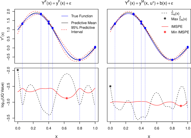
Figure 1: top panels: GP surfaces for field predictions given just field data (left) and field data combined with simulator data using KOH (right); bottom panels: Uncertainty quantifation and acquisition critiera corresponding to the pannels directly above.

The top left panel of Figure 1 shows the results of fitting a zero mean GP to a modest, but noisy, data set. Details for the data-generating mechanism(s) involved in this example are delayed until §3.2. The predictive mean and the true mean function, shown as the solid black and blue lines respectively, are fairly close together, illustrating decent accuracy. Red dashed lined indicate 95% predictive intervals, calculated from $\hat{\Sigma}_{N}(x)$ and shown as a dotted black line in the bottom left panel. Observe that the interval becomes wider, depicting higher uncertainty, in-between two training data locations.

2.2 Integrated Mean Squared Prediction Error

Those equations 3 have many uses: simply predicting at novel $x$ not coinciding with training runs $X$; deducing where $Y(x)$ might be minimized via Bayesian optimization (BO, Jones et al.,, 1998); exploring which coordinates of $x$ most influence $Y(x)$ (Marrel et al.,, 2009); to name just a few. Here we are interested in sequential experimental design, or active learning, to select new runs for an improved fit/prediction.

The simplest variation on this theme is to choose $\tilde{x}_{N+1}=\mathrm{argmax}_{x\in\mathcal{X}}\hat{\Sigma}_{N}(x)$, i.e., to maximize the predictive variance. Here $x$ and $\tilde{x}_{N+1}$ represent a single $N^{\prime}=1\times d$ coordinate vector in the input space $\mathcal{X}$, but the idea is easily generalized to larger batches. MacKay, (1992) showed that such acquisitions lead to (approximate) maximum entropy designs in the context of neural network surrogates, and Seo et al., (2000) extended these to GPs naming the idea active learning MacKay (ALM). Despite their simplicity, convenient closed form, and analytic gradients (not shown) for efficient library-based numerical optimization, ALM-based sequential designs are aesthetically limiting as they tend to concentrate new runs on the boundary of the input space $\mathcal{X}$. ALM is also inefficient for prediction unless the boundary is especially important to the application at hand.

If accuracy over the entirety of the input space $\mathcal{X}$ is desired then it helps to have a criterion that more squarely targets that objective. Sacks et al., (1989) proposed the integrated mean-squared prediction error (IMSPE) criterion, encapsulated generically as $\mathrm{IMSPE}(X)=\int_{\mathcal{X}}\hat{\Sigma}_{N}(x)\;dx$. Again $x$ is $1\times d$ so that the integral is $d$-dimensional. One could use this criterion to choose an entire $N\times d$ design $X$ in one shot by optimizing over all $Nd$ coordinates as in $\tilde{X}=\mathrm{argmin}_{X\in\mathcal{X}^{N}}\mathrm{IMSPE}(X)$, or to simply augment $X$ with a new row $x_{N+1}$ sequentially, in an active learning setting. Independently, Cohn, (1994) developed a similar criterion for neural network surrogates and one-at-a-time acquisition, approximating the integral as a sum; Seo et al., (2000) extended their work to GPs, dubbing this Active Learning Cohn (ALC). Variations abound (see §1).

Here we follow the mathematics laid out by Binois et al., (2019), who provided a closed form IMSPE and gradient under a uniform measure for $\mathcal{X}\in[0,1]^{d}$, i.e. $p(\mathcal{X})=\mathcal{U}[0,1]^{d}$. Their interest, like ours, was in active learning (i.e., acquisition of $x_{N+1}$) although their development is equally applicable to one-shot and batch design. The approach is at once elegant and practical in implementation, and consequently has spurred a cottage industry of variations (Wycoff et al.,, 2021; Cole et al.,, 2021; Sauer et al.,, 2022) of which our main contribution can be viewed as yet another. The derivation relies on two trace identities: $\mathrm{tr}(ABC)=\mathrm{tr}(BCA)$; and $\mathrm{tr}(AB)=1^{\top}(A\circ B)1$ where $1$ is a vector of ones with a length equal to the number of rows in $X$, and $\circ$ is the Hadamard, or element wise, product. It also involves a re-positioning of the integral inside of the matrix trace, which is legitimate as both are linear operators. A uniform measure yields closed forms for $W(X)=W(X,X)=\int_{[0,1]^{d}}k(X,x)k(X,x)^{\top}\;dx$ as an $N\times N$ under common kernels $k(\cdot,\cdot)$, which are not duplicated here. See the appendix of Binois et al., (2019). Combining those elements, and interpreting the integral as an expectation over uniform $x$, yields

$$\begin{split}\mathrm{IMSPE}(X)&=\int_{[0,1]^{d}}\nu k(x,x)-\nu k(x,X)^{\top}K(X)^{-1}k(X,x)\;dx\\ &=\nu-\int_{[0,1]^{d}}\mathrm{tr}\left(\nu K(X)^{-1}k(X,x)k(x,X)\right)\;dx\\ &=\nu-\nu 1^{\top}\left(K(X)^{-1}\circ W(X)\right)1.\end{split}$$ (4)

We introduce these techniques, and enhanced level of detail for a review, because our own work in §3 involves similar operations. In practice, estimates of $\nu$ maybe be used and those may involve $(X,Y_{N})$. However, the typical development presumes that we don’t have $Y$-values yet, or at least not $y_{N+1}$ in the active learning context. Consequently, it is equivalent to choose

$$\tilde{x}_{N+1}=\underset{x\in[0,1]^{d}}{\mathrm{argmin}}\ 1^{\top}\left(K(X)^{-1}\circ W(X)\right)1\quad\quad\mbox{ where }X\equiv[X;x^{\top}],$$ (5)

i.e., where $X$ is augmented with the new row $x^{\top}$. In this way, the acquisition explicitly targets predictive accuracy by minimizing mean-squared error. One consequence of this is that acquisitions avoid boundaries of $\mathcal{X}=[0,1]^{d}$ as that set has no volume relative to the interior being integrated over.

Returning to Figure 1, the bottom left plot allows for comparison of the dotted black line plotting predictive variance, and the solid red line plotting IMSPE as a function of the $x$ augmenting the initial design. The minimum IMSPE point, $\tilde{x}_{N+1}$ is a red asterisk. Observe that the input with the highest predictive variance, at the left boundary, does not agree with $\tilde{x}_{N+1}$.

2.3 Simulator calibration

Now suppose we have data from two experiments: a simulation campaign and measurements from an analogous physical/field apparatus. As a highly stylized concrete example, consider data described in Gramacy, (2020) §9.2, via a physics model and empirical observations of the time $t$ a ball would take to drop from a given height $h$. The model/simulator, described $t=\sqrt{2h/g}$ depends on an (unknown) gravitational constant $g$, and does not incorporate any other factors such as kinetic/wind resistance. The model can be freely evaluated for positive values of both $h$, and $g$. In the physical apparatus only the height $h$ can be easily controlled. So $g$ is a tuning parameter, and also one possibly doing double-duity to account for any other factors not in the model which would slow the ball down in its fall.

It makes sense to entertain modeling apparatus that can synthesize these two data sources: estimating an appropriate $g$ – not necessarily identifying its “true” value, because the model doesn’t incorporate all of the physics – and correcting the bias in the computer model in order to furnish accurate predictions for $t$ at any $h$ of interest. The KOH calibration model does this well. In our description here, and introduction of notation more general than the ball-drop example, we follow Bayarri et al., (2009). Let $Y^{M}([x_{1\times p},u_{1\times s}]_{1\times d})\equiv t=Y^{M}([h,g]_{1\times 2})$ for the simple example above. Put another way, an observation of the computer model, $Y^{M}(x,u)$, is simply equal to a function of $x_{1\times p}$ and a tuning parameter $u_{1\times s}$, where for the simple example $h\equiv x$ and $g\equiv u$. If the computer model is expensive to evaluate, a GP surrogate can be fit to a $N_{M}\times 1$ vector of observations $Y_{N_{M}}$ simulation campaign of inputs $[X_{N_{M}\times p},U_{N_{M}\times s}]$.

KOH assumes the real field observations at location $x$, $Y^{F}(x)$, can be modeled as a noisy realization of a computer model $y^{M}(x,u)$ set at the ideal/true value of $u=u^{\star}$ after correcting for the bias $b(x)$, or any systematic discrepancy inherent in the computer model:

$$Y^{F}(x) =y^{M}(x,u^{\star})+b(x)+\epsilon,\quad\epsilon\stackrel{{\scriptstyle\mathrm{iid}}}{{\sim}}\mathcal{N}(0,\sigma^{2}).$$ (6)

KOH places a GP prior on $b(\cdot)$ so that $\hat{b}(x)$ may be estimated jointly with $\hat{u}$ and $\hat{\sigma}^{2}$ based on observed discrepancies $b(x)=y^{F}-y^{M}(x,u)$ values from a simulation and field data campaign. Provided that a second GP is used as a surrogate for $Y^{M}(x,u)$, the joint marginal likelihood, governing prediction and hyperperameter inference, for field data $Y_{N_{F}}$, computer model runs $Y_{N_{M}}$, and predictive outputs $Y^{F}(x)\equiv Y^{F}(x,\hat{u})$ derives from multivariate normal, of dimension $N_{F}+N_{M}+1$ with mean zero and covariance matrix

$$\mathbb{C}\mathrm{ov}\left(\begin{bmatrix}Y^{F}(x,\hat{u})\\ Y_{N_{F}}\\ Y_{N_{M}}\end{bmatrix}\right)=\Sigma^{M}+\Sigma^{B}\quad\mbox{where}\quad\Sigma^{B}=\nu_{B}\begin{bmatrix}k^{B}{(x)}&k^{B}{(x,X_{N_{F}})}&0\\ k^{B}{(X_{N_{F}},x)}&K^{B}(X_{N_{F}})&0\\ 0&0&0\\ \end{bmatrix}$$ (7)

$$\mbox{and}\quad\Sigma^{M}=\nu_{M}\begin{bmatrix}k([x,\hat{u}])&k{([x,\hat{u}],[X_{N_{F}},\hat{U}])}&k{([x,\hat{u}],[X_{N_{M}},U_{N_{M}}])}\\ k{([X_{N_{F}},\hat{U}],[x,\hat{u}])}&K([X_{N_{F}},\hat{U}])&K([X_{N_{F}},\hat{U}],[X_{N_{M}},U_{N_{M}}])\\ k([X_{N_{M}},U_{N_{M}}],[x,\hat{u}])&K([X_{N_{M}},U_{N_{M}}],[X_{N_{F}},\hat{U}])&K([X_{N_{M}},U_{N_{M}}])\end{bmatrix}.$$

Above, additional subscripts $\nu_{M}$ and $\nu_{B}$ indicate separate scale hyperparameters for the surrogate and bias GPs, respectively. We use $k(\cdot)$ and $K(\cdot)$ for the computer model kernel and matrix evaluation, etc, and introduce $B$ superscripts for the bias analog. Implicit in $K^{B}(\cdot)$ as an additive diagonal $\mathbb{I}g$ so that a nugget parameter $g$ can capture noise with variance $\sigma^{2}=\nu_{B}g$. The two kernels may come from a similar family, but are uniquely hyperparmeterized, however this is suppressed from the notation for simplicity.

The predictive equations are derived in a manner similar to Eqs. 2–3, except resulting in a more complicated set of matrix–vector multiplications. The mean is not central to our discussion here, but form of the variance is important for calculating IMSPE. We have that

$$\hat{\Sigma}(x\mid\hat{u}) \equiv\mathbb{V}\mathrm{ar}(Y^{F}(x,\hat{u})\mid Y_{N_{F}},Y_{N_{M}})$$ (8)

$$=\nu_{M}k([x,\hat{u}])+\nu_{B}k^{B}{(x)}-\begin{bmatrix}\nu_{M}k+\nu_{B}k^{B}\end{bmatrix}^{\top}\begin{bmatrix}\Sigma^{M,B}_{N_{F}+N_{M}}\end{bmatrix}^{-1}\begin{bmatrix}\nu_{M}k+\nu_{B}k^{B}\end{bmatrix}$$

$$\mbox{where}\quad k =\begin{bmatrix}k{([X_{N_{F}},\hat{U}],[x,\hat{u}])}\\ k([X_{N_{M}},U_{N_{M}}],[x,\hat{u}])\end{bmatrix}\quad\quad\quad k^{B}=\begin{bmatrix}k^{B}{(X_{N_{F}},x)}\\ 0_{N_{M}}\end{bmatrix}$$

$$\Sigma^{M,B}_{N_{F}+N_{M}} =\begin{bmatrix}\nu_{M}K([X_{N_{F}},\hat{U}])+\nu_{B}K^{B}(X_{N_{F}})&\nu_{M}K([X_{N_{F}},\hat{U}],[X_{N_{M}},U_{N_{M}}])\\ \nu_{M}K([X_{N_{M}},U_{N_{M}}],[X_{N_{F}},\hat{U}])&\nu_{M}K([X_{N_{M}},U_{N_{M}}])\end{bmatrix}.$$

The top right panel of Figure 1 shows a GP fit using the same data in the top left plot, but augmented with simulator runs ($Y_{N_{M}},X_{N_{M}}$) using the KOH framework. This extra information results reduced predictive variance across the input space as indicated by comparing black dotted lines in the bottom panels. More data, even if the data is not field data, reduces predictive uncertainty. Further reductions could be realized with even more computer model runs, which is the target of our main methodological contribution.

3 Optimal acquisition of new simulator runs

Here we derive a closed form active learning criteria by deploying IMSPE in the KOH framework. Gradients are provided to facilitate efficient numerical optimization. These also yield additional insight into the value of potential new simulation runs. We extend our simple illustration to reveal the new acquisition landscape.

3.1 Closed form KOH-IMSPE and derivative

Predictive variance $\hat{\Sigma}(x\mid\hat{u})$ in hand 8, the key step in deriving a KOH-IMSPE acquisition criteria is to integrate over the input space of the field predictive location $x$. Throughout this discussion we condition on $(\hat{u},\hat{\nu}_{M},\hat{\nu}_{B})$ and any other relevant estimated hyperparameters, e.g., via a maximum a-posteriori (MAP) (e.g., Gramacy,, 2020, §9.1), which would be updated after each active learning acquisition. Our focus here is how to acquire new simulator runs given those values. Section §6 offers thoughts on how alternative hyperparameter estimation strategies might impact our active learning setup.

The series of equations below outlines our approach to integrating the predictive variance over $x$, beginning with an expansion of the quadratic form in Eq. 8. Hats are dropped on the estimated scales to reduce clutter. Although expressed here as a function of the computer model design $[X_{N_{M}+1},U_{N_{M}+1}]$, IMSPE would also depend upon the field data.

$$\mathrm{IMSPE} ([X_{N_{M}+1},U_{N_{M}+1}])=\int_{[0,1]^{p}}\hat{\Sigma}(x\mid\hat{u})\;dx$$

$$=\nu_{M}+\nu_{B}-\int_{[0,1]^{p}}\mathrm{tr}\left(\left[\Sigma^{M,B}_{N_{F}+N_{M}+1}\right]^{-1}\left(\nu_{M}^{2}kk^{\top}+2\nu_{M}\nu_{B}k^{B}k^{\top}+\nu_{B}^{2}k^{B}[k^{B}]^{\top}\right)\right)\;dx$$ (9)

$$=\nu_{M}+\nu_{B}-\int_{[0,1]^{p}}1^{\top}\left(\left[\Sigma^{M,B}_{N_{F}+N_{M}+1}\right]^{-1}\circ\left(\nu_{M}^{2}kk^{\top}+2\nu_{M}\nu_{B}k^{B}k^{\top}+\nu_{B}^{2}k^{B}[k^{B}]^{\top}\right)\right)1\;dx$$ (10)

$$=\nu_{M}+\nu_{B}-1^{\top}\left(\left[\Sigma^{M,B}_{N_{F}+N_{M}+1}\right]^{-1}\circ\left(\nu_{M}^{2}W^{M,M}+2\nu_{M}\nu_{B}W^{M,B}+\nu_{B}^{2}W^{B,B}\right)\right)1$$ (11)

Trace identity $\mathrm{tr}(ABC)=\mathrm{tr}(BCA)$ is involved in 9, whereas 10 utilizes $\mathrm{tr}(AB)=1^{\top}(A\circ B)1$. At this point within the derivation, $\hat{\Sigma}(x\mid\hat{u})$ has been broken into a weighted sum of the functions specifying the covariance between $x$ and the observations, providing a less abstract format for integration. Integration produces 11, where for any $\{\alpha,\beta\}\in\{M,B\}$: $W_{\alpha,\beta}=\int_{[0,1]^{p}}k_{\alpha}k_{\beta}^{\top}\;dx$. Solutions for the elements of $W_{\cdot,\cdot}$ are kernel-dependent. §A.1 provides forms compatible with Gaussian kernels. Similar derivations for Matérn kernels can be found in Binois et al., (2019).

Acquisition of a new computer model run $[\tilde{x},\tilde{u}]$ requires minimizing IMSPE 11 with the augmented design:

$$[\tilde{x},\tilde{u}]=\mathrm{argmin}_{[x,u]\in\mathcal{X}^{d}}\ \mathrm{IMSPE}([X_{N_{M}+1},U_{N_{M}+1}])\quad\mbox{where}\quad[X_{N_{M}+1},U_{N_{M}+1}]\equiv[X_{N_{M}},U_{N_{M}};x,u].$$ (12)

To continue with our running illustration, the bottom-right panel of Figure 1 shows KOH-IMSPE instead of typical IMSPE, but for the acquisition of an additional field data point instead of computer model point. Notably, IMSPE, along with predictive variance, is lower for the KOH GP fit. Because of the additional computer model data, the KOH-IMSPE surface is still multi-modal, but flat relative to the GP fit with only field data (bottom-left panel). Additionally, the point which minimizes IMSPE when computer simulator data is introduced is different than when no computer simulator data is used.

Considering the multi-modality of the KOH-IMSPE acquisition surface, and its relative flatness compared with ordinary IMSPE, a thoughtful strategy for solving the program in Eq. 12 is essential to obtaining good acquisitions. Local numerical optimization via finite differentiating in this setting can be fraught with numerical challenges. One option is to deploy a discrete candidate set for $\tilde{X}$, such as via LHS or triangulation (Gramacy et al.,, 2022). Our analytical elicitation of KOH-IMSPE 11 allows for the closed form derivatives for the purpose of gradient based minimization, as we describe below. Library-based (e.g., BFGS, Byrd et al., (1995)) optimizers using gradients can be deployed in a random multi-start scheme, or via candidates.

The derivative of KOH-IMSPE with respect to element $l$ of $[\tilde{x},\tilde{u}]$ is shown in Eq. 13. The fact that $[\tilde{x},\tilde{u}]$ is contained within $\Sigma^{M,B},W^{M,M},$ and $W^{M,B}$, necessitates the use of the chain rule for matrices and inverses:

$$\frac{\partial(U(x)\circ V(x))}{\partial x}=U(x)\circ\frac{\partial V(x)}{\partial x}+\frac{\partial U(x)}{\partial x}\circ V(x)\quad\mbox{ and }\frac{\partial U(x)^{-1}}{\partial x}=-U(x)^{-1}\frac{\partial U(x)}{\partial x}U(x)^{-1}.$$

Using these, we find that the derivative of KOH-IMSPE can be written as follows:

$$\frac{\partial\,\mathrm{IMSPE}}{\partial[\tilde{x},\tilde{u}]_{l}} =1^{\top}\left(\left[\Sigma^{M,B}_{N_{F}+N_{M}+1}\right]^{-1}\frac{\partial\Sigma^{M,B}_{N_{F}+N_{M}+1}}{\partial[\tilde{x},\tilde{u}]_{l}}\left[\Sigma^{M,B}_{N_{F}+N_{M}+1}\right]^{-1}\!\!\!\circ\left(\nu_{M}^{2}W^{M,M}+2\nu_{M}\nu_{B}W^{M,B}+\nu_{B}^{2}W^{B,B}\right)\right.-$$

$$\qquad\left.\left[\Sigma^{M,B}_{N_{F}+N_{M}+1}\right]^{-1}\!\!\!\circ\left(\nu_{M}^{2}\frac{\partial W^{M,M}}{\partial[\tilde{x},\tilde{u}]_{l}}+2\nu_{M}\nu_{B}\frac{\partial W^{M,B}}{\partial[\tilde{x},\tilde{u}]_{l}}\right)\right)1,$$ (13)

where forms for $\frac{\partial W^{M,M}}{\partial[\tilde{x},\tilde{u}]}$, $\frac{\partial W^{M,B}}{\partial[\tilde{x},\tilde{u}]}$, and $\frac{\partial\Sigma^{M,B}_{N_{F}+N_{M}+1}}{\partial[\tilde{x},\tilde{u}]}$ are provided in Appendices A.1 and A.2.

It is illuminating to study how this gradient behaves when $\tilde{u}=\hat{u}$. One might hypothesize that if KOH-IMSPE were to collect simulator data near $\hat{u}$, that the gradient of KOH-IMSPE would be near zero there. The first term in Eq. 13 can be rewritten as follows using Hadamard product and trace identities.

$$1^{\top}\frac{\partial\Sigma^{M,B}}{\partial\tilde{x}}\circ[\Sigma^{M,B}]^{-1}\left(\nu_{M}^{2}W^{M,M}+2\nu_{M}\nu_{B}W^{M,B}+\nu_{B}^{2}W^{B,B}\right)[\Sigma^{M,B}]^{-1}1$$

For the Gaussian kernel, taking $\frac{\partial\Sigma^{M,B}}{\partial\tilde{u}}$ and setting $\tilde{u}=\hat{u}$ produces a matrix of mostly zeros:

$$\frac{\partial\Sigma^{M,B}}{\partial\tilde{u}}:(\tilde{u}=\hat{u})=\nu_{M}\begin{bmatrix}0_{N_{F}\times N_{F}}&0_{N_{F}\times N_{M}}&0_{N_{F}\times 1}\\ 0_{N_{M}\times N_{F}}&0_{N_{M}\times N_{M}}&\left(\frac{\partial k([X_{M},U_{M}],[\tilde{x},\tilde{u}])}{\partial\tilde{u}}\right)_{N_{M}\times 1}\\ 0_{1\times N_{F}}&\left(\frac{\partial k([\tilde{x},\tilde{u}],[X_{M},U_{M}])}{\partial\tilde{u}}\right)_{1\times N_{M}}&0_{1\times 1}\end{bmatrix},$$ (14)

since $\partial k([\tilde{x},\tilde{u}],[X_{f},\hat{U}]|\tilde{u}=\hat{u})/\partial\tilde{u}\propto-\frac{2(\tilde{u}-\hat{u})}{\theta^{M}}\exp\left(-(\hat{u}-\tilde{u})^{2}/\theta^{M}\right)=0$. Any trace of the multiplication of the differential covariance matrix by another matrix will be near, but typically not located at, a minimum when $\tilde{u}=\hat{u}$. This result reveals a trade-off between exploratory behavior, away from $\hat{u}$, and exploitation nearby $\hat{u}$. We shall see this behavior manifest empirically in a moment. But first, observe that the second term in Eq. 13 is related to the change in the integrated covariance between $[x,\hat{u}]$, $[\tilde{x},\tilde{u}]$, and $[X_{N_{F}},\hat{U};X_{N_{M}},U_{N_{M}}]$. Interestingly, both $\frac{\partial W^{M,M}}{\partial\tilde{u}}$ and $\frac{\partial W^{M,B}}{\partial\tilde{u}}$ are equal to 0 when $\tilde{u}=\hat{u}$, which would reduce the second term in 13 to zero under the same conditions. In the full evaluation of 13, the location of a zero-value for the gradient in $U$-space balances the correlation between how close $[x,\hat{u}]$ is to $[\tilde{x},\tilde{u}]$, as well as the correlation between $[X_{N_{M}},U_{N_{M}}]$ and $[\tilde{x},\tilde{u}]$.

3.2 Illustration

Consider the following data-generating mechanism with 1d design input $(x)$ and 1d calibration parameter $(u)$.

$$y^{M}(x,u) =\sin(10x,u) b(x) =1-\frac{1}{3}x-\frac{2}{3}x^{2}$$

$$Y^{F}(x) =y_{m}\left(x,u^{\star}=\frac{\pi}{5}\right)+b(x)+\epsilon \epsilon \stackrel{{\scriptstyle\mathrm{iid}}}{{\sim}}\mathcal{N}(0,0.1^{2})$$

This example underpins the running illustrative example supported by Figure 1. The left panel of Figure 2 shows the mean of the field data $\mathbb{E}(Y^{F}(x))=y_{m}\left(x,u^{\star}=\frac{\pi}{5}\right)+b(x)$ juxtaposed against the computer model $y_{m}\left(x,u^{\star}=\frac{\pi}{5}\right)$, whereas the right panel shows how other settings of $u$ affect that computer model.

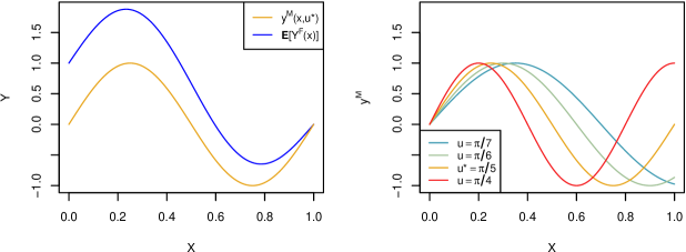
Figure 2: True surface, model surface with $u^{\star}$, and effect of varying $u$ on the model surface.

Here we explore the KOH-IMSPE on this example. To initialize, a $N_{M}=10$-sized 2d LHS was used for the initial computer model design in $[X,U]$-space. Field data was collected as two replicates of five unique locations (i.e., $N_{F}=10$) on an equally spaced grid on $X$. Following Bayarri et al., (2009) and Gramacy, (2020) §9.2, we fit a GP surrogate to the simulator data and bias GP to the residuals from the field data, thereby estimating $\hat{u}$ jointly with other hyperparameters via MAP with $p(u)=\mathrm{Beta}(2,2)$, a standard regularizing prior on the calibration parameter. We then proceeded with 25 KOH-IMSPE acquisitions of new computer model runs. After each acquisition the model(s) were re-fit to prepare for the next one.

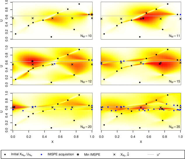
Figure 3: KOH-IMSPE surface in $X,U$ space as points are sequentially added to an initial computer model design. Red indicates lower values and white/yellow indicates larger values.

Figure 3 shows KOH-IMSPE surface plots for $N_{M}=$ 10, 11, 12, 15, 20, 35, the location of minimum KOH-IMSPE, the initial computer model design, and the points previously added via KOH-IMSPE. Red colors in the surface indicate smaller KOH-IMSPE values. The location of $u^{\star}$ is shown as a grey line, which is fixed in each panel. Field data locations are plotted at $(X_{N_{F}},\hat{u})$ for the estimate of $\hat{u}$ found at the given size of $N_{M}$, which is distinct in each panel. Observe that minimum KOH-IMSPE, i.e., $\tilde{u}$ solving Eq. 12 is often found near $\hat{u}$, but not always. Distinct exploratory behavior is still observed in the $u$-coordinate, i.e., reflecting the tradeoff between exploration and exploitation suggested by the analysis of derivative information at the end of §3.1. There are also a diversity of $x$-values, marginally.

4 Implementation and benchmarking

Code for all illustrative and benchmarking examples herein is in R and may be found in our Git repository https://bitbucket.org/gramacylab/kohdesign. Subroutines found therein liberally borrow from laGP (Gramacy,, 2016) and hetGP (Binois and Gramacy,, 2021) libraries to make predictions, find MAP estimates of kernel hyperparameters (under Gamma priors detailed later), to build covariance matrices, and evaluate integrals when appropriate. Throughout, inputs $[X,U]$ are scaled to $[0,1]$ to improve numerical stability and simplify code for the required integrals. Independent $\mathrm{Beta}(2,2)$ priors were used for each element of $u$, throughout, and MAP solutions under a modularized KOH Bayarri et al., (2007) yielded $\hat{u}$ estimates were provided via optim(..., gr=NULL, method="Nelder-Mead") (Nelder and Mead,, 1965) or optim(..., gr=NULL, method="Brent") (Brent,, 2013) subroutines, as described by Gramacy et al., (2015) and demonstrated in Gramacy, (2020) §9.1.

Our implementation of the numerical calculation of closed form Eq. 11 is faithful to the description detailed in Appendix A.1. To enhance stability, and reduce computation time involved in the search of the next acquisition, $[\tilde{x},\tilde{u}]$ solving, 5, closed form gradients (i.e., non-NULL settings gr) are supplied to optim(..., gr, method="L-BFGS-B"). These are also furnished in A.1, including gradients of all $W^{\cdot,\cdot}$ values, as required. To further reduce computation time, block matrix inversion (Bernstein,, 2009) of $\Sigma^{M,B}$ was utilized to avoid full covariance matrix inversion for every candidate entertained by the optimizer. However, block matrix inversion substantially complicates the expressions for gradients. These additional details are provided in Appendix A.2. To detail with the multi-modality of the KOH-IMSPE surface, our optim calls are wrapped in a multi-start scheme initialized at the best inputs found on a discrete LHS candidate set.

The remainder of this section describes two synthetic, Monte Carlo (MC), benchmarking exercises where actively learned KOH-IMSPE designs are compared to three space-filling alternatives: LHS, uniformly random, and a sequential IMSPE design for learning the computer model independent of the field data. We call this comparator M-IMSPE, and it is calculated via hetGP::IMSPE_optim(..., h=0)$par. Everything is re-randomized for each MC iteration. Initial computer model designs of size $N_{M_{0}}$ are chosen as random subset of the full LHS design. To control variability, identical (but random to each MC iteration) field data is shared between each method. After each active learning acquisition GP hyperparameters and $\hat{U}$ were updated. A natural metric for comparing these designs is $\mathrm{RMSE}=\sqrt{\frac{1}{N}\sum^{N}_{i=1}(\mu(x_{i})-y_{i})^{2}}$ calculated on the predictions $\mu(x_{i})$ from each method against a hold-out set of (de-noised) field data outputs $y_{1},\dots,y_{N}$. These RMSE values are saved after each acquisition, or as each additional element of the uniform/LHS is incorporated. We explore how the the distribution of these RMSE values changes as budgets $N_{M}$ are increased from $N_{M_{0}}$ up to a final stopping budget determined ex-post after the best of the method(s) seem to have converged.

4.1 Sinusoid

Our first benchmarking example was used as the basis of our running illustration, with details provided in §3.2. We entertained 1000 MC repetitions using $N_{M_{0}}=10$ initial space-filling design points and a final budget of $N_{M}=50$. Priors on GP hyperparameters were: $p(\theta^{M})=\mathrm{Gamma}(3/2,2)$, $p(\theta^{B})=\mathrm{Gamma}(3/2,5)$, $p(g_{B})=\mathrm{Gamma}(3/2,7)$. For each MC iteration a fixed, evenly spaced grid of 10 field data points was evaluated twice, providing $N_{F}=20$ unique (randomly generated) values. RMSE for field predictions was computed using a 100-point LHS test set, common to each method but novel to each MC iteration.

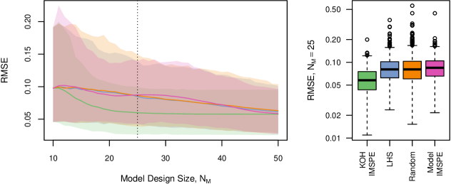
Figure 4: Left: mean RMSE and 90% quantiles for sinusoid data generating mechanism using KOH-IMSPE, LHS, random uniform, and M-IMSPE designs. Vertical line indicates the $N_{M}$ for the boxplot on the Right.

Figure 4 summarizes these RMSEs in two views. The left panel shows mean RMSE and 90% quantiles over $N_{M}$. There is high variability in the results which may be attributed to the low signal/noise ratio in the field data relative to computer model runs. Even so, after the addition of just a few points, KOH-IMSPE clearly outperforms its competitors on average. The right panel in the figure provides more resolution on the comparison of distributions of RMSE at the particular design size of $N_{M}=21$. Observe that the upper quartile of KOH-RMSE is below the median of all other methods. Also, there are no extreme RMSE outliers, whereas the others can perform quite poorly depending on how they are randomly initialized.

Interestingly, with this example, there is little difference in performance between the model based M-IMSPE and the model independent space-filling designs. Focusing on improving computer model prediction accuracy does not always translate into improved field predictions. Estimation risk is the culprit here. Relying on quality estimators of variance in low-signal settings to fine-tune space-fillingness in a design is risky compared to targeting space-fillingness geometrically. In higher-dimensional settings (as we shall see momentarily), where notions of space-filling by variance are more nuanced, there is more scope for improvement.

4.2 Goh/Bastos problem

Our second example comes from Goh et al., (2013), which is adapted from Bastos and O’Hagan, (2009), but our treatment most closely resembles the slightly simpler setup described in exercise 2 from §8 of Gramacy, (2020). It involves a 2d design space ($x$) and 2d calibration parameter ($u$). The data-generating mechanism is described as follows, where $u^{\star}=(0,2,0.1)$.

$$y^{M}(x,u) =\left(1-\exp\left(-\frac{1}{2x_{2}}\right)\right)\frac{1000u_{1}x_{1}^{3}+1900x_{1}^{2}+2092x_{1}+60}{100u_{2}x_{1}^{3}+500x_{1}^{2}+4x_{1}+20} b(x) =\frac{10x_{1}^{2}+4x_{2}^{2}}{50x_{1}x_{2}+10}$$

$$Y^{F}(x) =y^{M}\left(x,u^{\star}=[0.2,0.1]\right)+b(x)+\epsilon \epsilon \stackrel{{\scriptstyle\mathrm{iid}}}{{\sim}}\mathcal{N}(0,0.25^{2})$$

We performed 100 MC repetitions with $N_{M_{0}}$ = 30 and the final $N_{M}=130$. Field data was observed at 25 unique locations on an evenly spaced grid in $X\in[0,1]^{2}$, with two replicates at each for a total of $N_{F}=50$. Priors for hyperparameters were as follows: $p(\theta^{M})=\mathrm{Gamma}(3/2,5/4)$, $p(\theta^{B})=\mathrm{Gamma}(3/2,5/2)$, $p(g_{B})=\mathrm{Gamma}(3/2,1/20)$. RMSEs were calculated on an out-of-sample (noise-free) testing set on novel 1000-sized LHSs for each repetition.

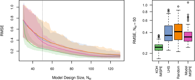
Figure 5: Left: mean RMSE and 90% quantiles for data generating mechanism from Gramacy, (2020) (Ch 8, Ex 2) using KOH-IMSPE, LHS, random uniform, and M-IMSPE designs. Vertical line indicates the $N_{M}$ for the boxplot on the Right.

Figure 5 shows the results in the same layout as Figure 4. Observe that from $N_{M}=31$ to around $N_{M}=40$ there is little discernible difference in RMSE between LHS, random, and M-IMSPE designs. However, mean RMSE for KOH-IMSPE quickly dominates, and bounds for its 90% quantile are much narrower at the beginning of each repetition. The worst case RMSEs for KOH-IMSPE are almost always better than the median RMSE for the other methods. Shortly after $N_{M}=40$ M-IMSPE shows consistent improvement over the randomized space-filling methods, but M-IMSPE requires the acquisition of another 70 data points before the method is competitive with KOH-IMSPE. Clearly, model based active learning is advantageous in this example, with KOH-IMSPE quickly providing the largest benefit for improving accuracy of field predictions.

5 Solvent extraction of rare Earth elements

Here we provide the results of testing the predictive accuracy of a KOH-IMSPE design on our motivating REE problem. We have a small, $N_{F}=$ 27-sized field data set. For these laboratory tests, three quantities $x$ (coded to $[0,1]^{3}$) were varied: the ratio of organic to aqueous liquids, and the mols and volume of sodium hydroxide (NaOH) solution used to adjust solution pH. We focus here on modeling the concentration of lanthanum (La) in the water-based aqueous phase, our output $y$-variable. Simulation of this quantity requires four (additional) chemical kinetic constants, calibration parameters $u$ (coded to $[0,1]^{4}$). Surrogate modeling therefore requires the exploration of a 7d $(x,u)$-space. Each run outputs elemental concentrations after approximating the solution of a set of differential equations through a Runge-Kutta routine. The simulator was run at a low fidelity due to the intensive nature of the MC experiment, resulting in a computation time of around 3.65 seconds on an 8-core Apple M1 Pro leveraging Apple vecLib. Data from the MC experiment was obtained from multiple computers and had total processor time of approximately 3.5 weeks. Further technical details can be found in Appendix B; our R implementation may be found in our repository along with other materials to reproduce these experiments.

To manage expectations, we remark that $N_{F}=27$ is very small in a seven-dimensional space. This has three consequences: (1) predictions on these field data lean heavily on computer model simulations; (2) information about promising $u$-values is weak; (3) scope for out-of-sample assessment of accuracy is limited and will have high MC error. Any design which is space-filling in $u$ coordinates will perform about as well as expected, leaving little scope for improvement with fancier alternatives, like KOH-IMSPE. Nevertheless, we argue that a KOH-IMSPE active learning strategy is worthwhile.

In each trial of our MC experiment, set up similarly to those in §4, we randomly held out 5 field data runs for out-of-sample RMSE assessments, so actually we used $N_{F}=$ 22. We entertained an initial simulation design of size $N_{M_{0}}=$ 50, and active learning up to $N_{M}=$ 300. Independent priors were as follows: $p(\theta_{M})=p(\theta^{B})=\mathrm{Gamma}\left(3/2,9/10\right),p(g)=\mathrm{Gamma}\left(3/2,1/20\right)$, and a $\mathrm{Beta}\left(2,2\right)$ on each coordinate of $u$. We performed a total of 500 MC trials, each with a unique train-test partition and initial LHS.

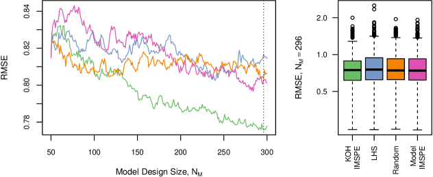
Figure 6: Left: mean RMSE calculated on a hold-out set for the SX application using KOH-IMSPE, LHS, random uniform, and M-IMSPE designs. Vertical line indicates the $N_{M}$ for the boxplot on the Right.

A plot of the average RMSE on the hold-out set is shown in the left panel of Figure 6. Error bars are removed to reduce clutter. Rather, we report that the signal-to-noise is low on these RMSE values, as can be seen in the boxplots in the right (note the change of scale on the $y$-axis), for $N_{M}=296$. Nevertheless, it is plain to see in the left panel that, on average, KOH-IMSPE outperforms its comparators. The boxplots indicate that it is important to assess the statistical significance of this visual comparison. At $N_{M}=296$ a one-sided paired Wilcoxon test of KOH-IMSPE versus M-IMSPE (the second-best by mean) rejects the null by most conventional levels with a $p$-value of $1.079\times 10^{-4}$.

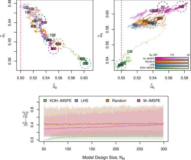
Figure 7: top panels: Mean path to convergence of $\hat{u}$ for various designs used in the SX application. Initial and final estimates are circled. Prior modes are shown as a red dashed line. bottom panel: Mean and 90% quantiles of squared distance between $\hat{u}$ and $\tilde{u}\mid\hat{u}$ for increasing $N_{M}$.

To further convince ourselves that our KOH-IMSPE designs are doing something interesting, we produced the plots Figure 7. These are inspired by Figure 3, which involved a more straightforward setup with one-dimensional $u$. Visuals in 4d are more complex. The top panel of Figure 7 shows the mean path of $\hat{u}$ as $N_{M}$ increases. For every design type, the path line starts as an off-white color when $N_{M}=50$, and becomes darker as $N_{M}$ approaches 300. Observe that the estimates obtained by the space-filling designs stay near, or take their time venturing away from the initial $\hat{u}$ obtained at $N_{M}=50$. By contrast, KOH-IMSPE quickly converges on a different subset of the space. Computer model acquisitions focused on improving prediction accuracy in the field improves convergence on $\hat{u}$, which helps reduce RMSE [Figure 6].

The bottom panel of Figure 7 provides some insight as to why KOH-IMSPE acquisition leads to more efficient $\hat{u}$ convergence. This plot provides mean squared distances and 90% quantiles between $\hat{u}$ and the subsequent acquisition $\tilde{u}$. It is worth remarking that that LHS, Random, and M-IMSPE do not utilize $\hat{u}$ to find $\tilde{u}$. Therefore, for these space-filling design types $||\tilde{u}-\hat{u}||^{2}_{2}$ is primarily related to how far each element of $\hat{u}$ is from 0.5. Observe that KOH-IMSPE, on the other hand, first collects points that are quite close to $\hat{u}$, with little variation. Then, as $N_{M}$ increases, GP hyperparameters converge, and RMSE decreases, the variation in $||\tilde{u}-\hat{u}||^{2}_{2}$ increases. We attribute this exploratory behavior to weight of the non-zero vectors in Eq. 14. These increase – become more important – with increasing $N_{M}$, pulling the location of the modes of KOH-IMSPE away from $\hat{u}$. Such exploratory behavior helps guard against pathologically bad estimates of $\hat{u}$, avoiding a vicious cycles that can plague active learning endeavors, especially in low-signal settings.

6 Discussion

Active learning is a weapon tool in the computer simulation experiment arsenal. When computers are involved, the scope for human-free automation is higher than in other settings where experimentation is required. Design strategies governed by active learning criteria have the potential to reduce data related expenses in the pursuit of achieving a specific goal. In the KOH calibration setting, it seems sensible to automate the design of a simulation campaign toward low-variance prediction in the field. Intuitively, the calibration parameter $u$, or estimates thereof $\hat{u}$, would affect such active learning criteria. We showed that it does, both technically (via the closed form of a variance-based acquisition criteria, KOH-IMSPE) and empirically in several illustrative and real-world examples.

There are, of course, other design goals that might be of interest, i.e., beyond reduced predictive variance. We remarked in §1 that identifiability/confounding is a concern with KOH. It may be that such confounding can be diminished, or controlled, with the right active learning criteria. This could be an important target of future research. Other potential add-ons might include batch acquisition for distributed simulation environments. It is natural to wonder if similar active learning principles could fruitfully be deployed to augment field data campaigns. Our initial experiments with this setup, admittedly using a cruder numerical IMSPE calculation, suggested a much lower return on investment in this setting. Even in highly stylized examples, we could not detect any difference (visual or empirical) between such designs and ordinary space-filling ones. There may be less scope for human-free automation in the design of field experiments in the KOH setting. However, an interesting twist to batch KOH-IMSPE would be the joint augmentation of both field and simulator data, for cases when more simulations can be run concurrent to the collection of additional field data. In this setup there may be further scope for automating aspects of design.

Turning now to our motivating application, use of KOH-IMSPE for active learning of SX processes has the potential to lead to insights for improving the extraction and concentration of the REEs necessary to provide widespread adoption of green technologies. Results from our study show that KOH-IMSPE has the capability to improve predictive accuracy of SX equilibrium concentrations utilizing less simulator data. The SX application illustrated is relatively simple, as only one REE was modeled, but nonetheless shows promise. Incorporating all REEs would lead to an even higher dimensional calibration parameter space. A more complex model would require more real/field data experimentation.

In the SX example, we had some difficulties evaluating the gradient of KOH-IMSPE in a numerically stable fashion. We were able to work around these with careful engineering, but these “hacks” may compromise the portability of our subroutines. Using better conditioned Matérn covariance functions (Stein,, 1999) may provide more stable gradient evaluations. Bayesian inference of $\hat{u}$ coupled with an efficient evaluation of KOH-IMSPE criteria may provide improvements due to to further uncertainty quantification of the calibration parameter in small field data settings. Additionally, Bayesian optimization (Jones et al.,, 1998) could be used to maximize the likelihood of $\hat{u}$ while probing the simulator input space, possibly allowing for reduced data requirements for convergence on $\hat{u}$. For simulators with multiple outputs a KOH-IMSPE criteria used with a cokriging model (Ver Hoef and Barry,, 1998) may be able to leverage larger amounts of information at each point for improved convergence of the calibration parameter.

Acknowledgements

This work supported, in part, by the U.S. Department of Energy, Office of Science, Office of Advanced Scientific Computing Research and Office of High Energy Physics, Scientific Discovery through Advanced Computing (SciDAC) program under Award Number 0000231018; and by National Science Foundation award CMMI-2152679.

Appendix A Kennedy and O’Hagan IMSPE Derivations

A.1 Integrals

Details are provided for evaluating the integrals required to calculate KOH-IMSPE in closed form when the GPs used in modeling the computer simulation and bias function both utilize a separable Gaussian covariance kernel. The provided derivations are for a uniformly rectangular $X$ space with inputs scaled to $[0,1]^{p}$ and a model conditioned on a point estimate of $\hat{U}$. The form for the integral is shown as 15 multiplied by 16, and can also be noted as the Hadamard product $W^{\alpha,\beta}(X)\circ W^{\alpha,\beta}(U)$ Below, the variables $\alpha,\beta$ express the combinations of the model and bias covariance kernels $(M,M);(M,B);(B,B)$, $i,j$ indexes all data locations from 1 to $N_{F}+N_{M}$, and $x,\hat{u}$ without an $i,j$ subscript is the field data predictive location.

$$w^{\alpha,\beta}_{i,j} =\int_{[0,1]^{p}}k^{\alpha}([x_{i},u_{i}],[x,\hat{u}])k^{\beta}([x,\hat{u}],[x_{j},u_{j}])dx_{1},\dots dx_{p}$$

$$=\prod_{l=1}^{p}\int_{0}^{1}\exp\left(-\frac{(x_{i,l}-x_{l})^{2}}{\theta^{\alpha}_{l}}\right)\exp\left(-\frac{(x_{j,l}-x_{l})^{2}}{\theta^{\beta}_{l}}\right)dx_{l}$$ (15)

$$\qquad\quad\times\prod_{l=p+1}^{d}\exp\left(-\frac{(u_{i,l}-\hat{u}_{l})^{2}}{\theta^{\alpha}_{l}}\right)\exp\left(-\frac{(u_{j,l}-\hat{u}_{l})^{2}}{\theta^{\beta}_{l}}\right)$$ (16)

To make notation simple and more compact, we do not state the bounds of integration going forward, and integrals should always be assumed to be evaluated from 0 to 1. This important note is not repeated again and again below in order to make the text more compact. For compactness we assume that $N_{M}$ contains the point augmented to the collected data for a sequential design application in this section.

Derivatives are provided for a gradient based search of the additional computer model point $[\tilde{x},\tilde{u}]$ which minimizes KOH-IMSPE. The expressions provided must be multiplied by remaining $d-1$ elements of the products 15 and 16. For example, for $l=2=p;d=3$ find $\frac{\partial W^{M,M}}{\partial\tilde{x}_{2}}=W^{M,M}(X_{1})\circ\frac{\partial W^{M,M}(X_{2})}{\partial\tilde{x}_{2}}\circ W^{M,M}(U_{1})$, while only the expression for $\frac{\partial W^{M,M}(X_{2})}{\partial\tilde{x}_{2}}$ is provided below.

A.1.1 $W^{M,M}$

The integral to be solved in order to find $W^{M,M}$:

$$W^{M,M}=\begin{bmatrix}\int k([X_{N_{F}},\hat{U}],[x,\hat{u}])k([x,\hat{u}],[X_{N_{F}},\hat{U}])dx&\int k([X_{N_{F}},\hat{U}],[x,\hat{u}])k([x,\hat{u}],[X_{N_{M}},U_{N_{M}}])dx\\ \int k([X_{N_{M}},U_{N_{M}}],[x,\hat{u}])k([x,\hat{u}],[X_{N_{F}},\hat{U}])dx&\int k([X_{N_{M}},U_{N_{M}}],[x,\hat{u}])k([x,\hat{u}],[X_{N_{M}},U_{N_{M}}])dx\end{bmatrix}$$ (17)

The $(i,j)^{\mathrm{th}}$ element of $w^{M,M}$ corresponding to x and 15 can be found as:

$$w^{M,M}_{i,j}(x)=\prod_{l=1}^{p}\frac{\sqrt{2\pi\theta^{M}_{l}}}{4}\exp\left(-\frac{(x_{i,l}-x_{j,l})^{2}}{2\theta_{l}^{M}}\right)\left(\mathrm{erf}\left(\frac{2-(x_{i,l}+x_{j,l})}{\sqrt{2\theta_{l}^{M}}}\right)+\mathrm{erf}\left(\frac{x_{i,l}+x_{j,l}}{\sqrt{2\theta_{l}^{M}}}\right)\right)$$ (18)

Where $\mathrm{erf}()$ is the Gauss error function. Elements of $W^{M,M}$ related to $U$ space and the product 16 can be found as 19, where $W^{M,M}=W^{M,M}(X)\circ W^{M,M}(U)$, and $J_{N_{F}\times N_{F}}$ is a square matrix of ones with a dimension of $N_{F}$

$$W^{M,M}(U)=\begin{bmatrix}J_{N_{F}\times N_{F}}&1_{N_{F}}k(\hat{u},U_{N_{M}})\\ k(U_{N_{M}},\hat{u})1^{\top}_{N_{F}}&k(U_{N_{M}},\hat{u})k(\hat{u},U_{N_{M}})\end{bmatrix}$$ (19)

Differentiation of $W^{M,M}$ is required to supply the optimization routine a gradient for minimization. Note, that only the last column and row of $\frac{\partial W^{M,M}}{\partial[\tilde{x},\tilde{u}]_{l}}\ \forall:l$ are non-zero. Differentiating with respect to an $\tilde{x}_{l}$ changes the $l^{\mathrm{th}}$ element of the product in 18 into the following:

$$\begin{split}\frac{\partial w^{M,M}(x_{i,l},\tilde{x}_{l})}{\partial\tilde{x}_{l}}&=\sqrt{\frac{\pi}{2}}\exp\left(-\frac{(x_{i,l}-\tilde{x}_{l})^{2}}{2\theta^{M}_{l}}\right)\left((x_{i,l}-\tilde{x}_{l})\frac{\mathrm{erf}\left(\frac{2-(x_{i,l}-\tilde{x}_{l})}{\sqrt{2\theta^{M}_{l}}}\right)+\mathrm{erf}\left(\frac{x_{i,l}+\tilde{x}_{l}}{\sqrt{2\theta^{M}_{l}}}\right)}{2\sqrt{\theta^{M}_{l}}}+\right.\\ &\left.\phantom{\frac{\mathrm{erf}\left(\frac{2-(x_{i,l}-\tilde{x}_{l})}{\sqrt{2\theta^{M}_{l}}}\right)}{2\sqrt{\theta^{M}_{l}}}}\frac{1}{2}\sqrt{\frac{2}{\pi}}\left(\exp\left(-\frac{(x_{i,l}+\tilde{x}_{l})^{2}}{2\theta^{M}_{l}}\right)-\exp\left(-\frac{(2-x_{i,l}-\tilde{x}_{l})^{2}}{2\theta^{M}_{l}}\right)\right)\right)\end{split}$$

However, for the case where $x_{i,l}=\tilde{x}_{l}$ (the bottom right corner of $W^{M,M}$), instead the derivative in 20 should be used.

$$\frac{\partial w^{M,M}(\tilde{x}_{l},\tilde{x}_{l})}{\partial\tilde{x}_{l}}=\exp\left(-\frac{2\tilde{x}_{l}^{2}}{\theta^{M}_{l}}\right)-\exp\left(-\frac{2(\tilde{x}_{l}-1)^{2}}{\theta^{M}_{l}}\right)$$ (20)

Differentiation with respect to $U$ space produces the following matrix, which similar to 19 should be element wise multiplied by the remaining functions evaluated to create $W^{M,M}$ related to the remaining $d-1$ dimensions of the input space.

$$\frac{\partial W^{M,M}(U)}{\partial\tilde{u}_{l}}=\begin{bmatrix}0_{N_{F}\times N_{F}}&0_{(N_{F}-1)\times(N_{M}-1)}&1_{N_{F}}\frac{\partial k(\hat{u},\tilde{u})}{\partial\tilde{u}_{l}}\\ 0_{(N_{M}-1)\times N_{F}}&0_{(N_{M}-1)\times(N_{M}-1)}&k(U_{N_{M}-1},\hat{u})\frac{\partial k(\hat{u},\tilde{u})}{\partial\tilde{u}_{l}}\\ 1_{N_{F}}^{\top}\frac{\partial k(\tilde{u},\hat{u})}{\partial\tilde{u}_{l}}&k(\hat{u},U_{N_{M}-1})\frac{\partial k(\tilde{u},\hat{u})}{\partial\tilde{u}_{l}}&\frac{\partial k(\tilde{u},\hat{u})}{\partial\tilde{u}_{l}}k(\hat{u},\tilde{u})+k(\tilde{u},\hat{u})\frac{\partial k(\hat{u},\tilde{u})}{\partial\tilde{u}_{l}}\end{bmatrix}$$ (21)

A.1.2 $W^{M,B}$

$$W^{M,B}=\begin{bmatrix}\int k([X_{N_{F}},\hat{U}],[x,\hat{u}])k^{B}(x,X_{N_{F}})dx&0_{N_{F}\times N_{M}}\\ \int k([X_{N_{M}},U_{N_{M}}],[x,\hat{u}])k^{B}(x,X_{N_{F}})dx&0_{N_{M}\times N_{M}}\end{bmatrix}$$ (22)

Solving for 22 requires particular attention to the fact that $k$ and $k^{B}$ have different lengthscale values ($\theta^{M}_{l}$ and $\theta^{B}$) for the same dimension. The result is shown below, where $x_{j}$ is always taken to be to the field data and from the bias kernel.

$$\begin{split}w^{M,B}_{i,j}(x)&=\prod_{l=1}^{p}\exp\left(-\frac{(x_{j,l}-x_{i,l})^{2}}{\theta^{B}_{l}+\theta_{l}^{M}}\right)\left(\frac{1}{2}\sqrt{\pi\left(\frac{1}{\theta_{l}^{M}}+\frac{1}{\theta^{B}_{l}}\right)^{-1}}\right)\left(\mathrm{erf}\left(\frac{\left(\frac{\theta^{B}_{l}x_{i,l}+\theta_{l}^{M}x_{j,l}}{\theta^{B}_{l}+\theta_{l}^{M}}\right)}{\sqrt{\left(\frac{1}{\theta_{l}^{M}}+\frac{1}{\theta^{B}_{l}}\right)^{-1}}}\right)\right.\\ &\qquad-\left.\mathrm{erf}\left(\frac{\left(\frac{\theta^{B}_{l}x_{i,l}+\theta_{l}^{M}x_{j,l}}{\theta^{B}_{l}+\theta_{l}^{M}}\right)-1}{\sqrt{\left(\frac{1}{\theta_{l}^{M}}+\frac{1}{\theta^{B}_{l}}\right)^{-1}}}\right)\right)\end{split}$$ (23)

Functions related to $U$ space can be found as24, where $W^{M,B}=W^{M,B}(X)\circ W^{M,B}(U)$, and $J_{N_{F}\times N_{F}}$ is a square matrix of ones with a dimension of $N_{F}$,

$$W^{M,B}(U)=\begin{bmatrix}J_{N_{F}\times N_{F}}&0_{N_{F}\times N_{M}}\\ k(U,\hat{u})1^{\top}_{N_{F}}&0_{N_{M}\times N_{M}}\end{bmatrix}$$ (24)

Differentiation of 23 with respect to $\tilde{x}$ for gradient based minimization of KOH-IMSPE produces:

$$\begin{split}&\frac{\partial w^{M,B}(\tilde{x}_{l},x_{j,l})}{\partial\tilde{x}_{l}}=\\ &\frac{e^{-\frac{(\tilde{x}_{l}-x_{j,l})^{2}}{\theta^{B}_{l}+\theta_{l}^{M}}}}{\theta_{l}^{M}+\theta^{B}_{l}}\left(\sqrt{\pi\left(\frac{1}{\theta^{B}_{l}}+\frac{1}{\theta_{l}^{M}}\right)^{-1}}(x_{j,l}-\tilde{x}_{l})\left(\mathrm{erf}\left(\frac{\left(\frac{\theta_{l}^{M}x_{j,l}+\theta^{B}_{l}\tilde{x}_{l}}{\theta_{l}^{M}+\theta^{B}_{l}}\right)}{\sqrt{\left(\frac{1}{\theta_{l}^{M}}+\frac{1}{\theta^{B}_{l}}\right)^{-1}}}\right)-\mathrm{erf}\left(\frac{\left(\frac{\theta_{l}^{M}x_{j,l}+\theta^{B}_{l}\tilde{x}_{l}}{\theta_{l}^{M}+\theta^{B}_{l}}\right)-1}{\sqrt{\left(\frac{1}{\theta_{l}^{M}}+\frac{1}{\theta^{B}_{l}}\right)^{-1}}}\right)\right)+\right.\\ &\left.\phantom{\mathrm{erf}\left(\frac{\left(\frac{\theta_{l}^{M}x_{j,l}+\theta^{B}_{l}\tilde{x}_{l}}{\theta_{l}^{M}+\theta^{B}_{l}}\right)}{\sqrt{\left(\frac{1}{\theta_{l}^{M}}+\frac{1}{\theta^{B}_{l}}\right)^{-1}}}\right)}\theta^{B}_{l}\left(e^{-\frac{\left(\frac{1}{\theta_{l}^{M}}+\frac{1}{\theta^{B}_{l}}\right)(\theta_{l}^{M}x_{j,l}+\theta^{B}_{l}\tilde{x}_{l})^{2}}{(\theta_{l}^{M}+\theta^{B}_{l})^{2}}}-e^{-\left(\frac{1}{\theta_{l}^{M}}+\frac{1}{\theta^{B}_{l}}\right)\left(\frac{\theta_{l}^{M}x_{j,l}+\theta^{B}_{l}\tilde{x}_{l}}{\theta_{l}^{M}+\theta^{B}_{l}}-1\right)^{2}}\right)\right)\end{split}$$

Once again, because of the form of 22, $x_{j}$ only corresponds to field data from the bias covariance functions

$$\frac{\partial W^{M,B}(U)}{\partial\tilde{u}_{l}}=\begin{bmatrix}0_{N_{F}\times N_{F}}&0_{N_{F}\times(N_{M})}\\ 0_{(N_{M}-1)\times N_{F}}&0_{(N_{M}-1)\times N_{M}}\\ \frac{\partial k(\tilde{u},\hat{u})}{\partial\tilde{u}_{l}}1^{\top}_{N_{F}}&0_{1\times 1}\end{bmatrix}$$

A.1.3 $W^{B,B}$

$$W^{B,B}=\begin{bmatrix}\int k^{B}(X_{N_{F}},x)k^{B}(x,X_{N_{F}})dx&0_{N_{F}\times N_{M}}\\ 0_{N_{M},\times N_{F}}&0_{N_{M}\times N_{M}}\end{bmatrix}$$

Evaluation of all entries in $W^{B,B}$ is only related to $X$ space. For the Gaussian kernel, the integral required for evaluation is equivalent to 18. In the search to find the additional data point $\tilde{x}$ which minimizes KOH-IMSPE, $\frac{\partial W^{B,B}}{\partial\tilde{x}}=0$. If acquiring field data while utilizing the information obtained from a computer simulator, derivatives would be equivalent to those for $W^{M,M}(X)$.

A.2 Block Matrix Inversion

Let:

$$\Sigma^{M,B}_{N_{F}+N_{M}+1}=\begin{bmatrix}\Sigma^{M,B}_{N_{F}+N_{M}}&\nu_{M}\tilde{k}\\[5.0pt] \nu_{M}\tilde{k}^{\top}&\nu_{M}k([\tilde{x},\tilde{u}])\end{bmatrix}$$

Where:

$$\tilde{k}=\begin{bmatrix}k([X_{N_{F}},\hat{U}],[\tilde{x},\tilde{u}])\\[5.0pt] k([X_{N_{M}},U_{N_{M}}],[\tilde{x},\tilde{u}])\end{bmatrix}$$ (25)

We can then find $[\Sigma_{N_{F}+N_{M}+1}^{M,B}]^{-1}$ as such:

$$[\Sigma_{N_{F}+N_{M}+1}^{M,B}]^{-1}=\begin{bmatrix}\kern 2.0pt[\Sigma^{M,B}_{N_{F}+N_{M}}]^{-1}+\frac{1}{b}\nu_{M}^{2}[\Sigma^{M,B}_{N_{F}+N_{M}}]^{-1}\tilde{k}\tilde{k}^{\top}[\Sigma^{M,B}_{N_{F}+N_{M}}]^{-1}&-\frac{1}{b}\nu_{M}[\Sigma^{M,B}_{N_{F}+N_{M}}]^{-1}\tilde{k}\kern 2.0pt\\[5.0pt] \kern 2.0pt-\frac{1}{b}\tilde{k}^{\top}[\Sigma^{M,B}_{N_{F}+N_{M}}]^{-1}&\frac{1}{b}\kern 2.0pt\end{bmatrix}$$ (26)

Where $b=\nu_{M}k([\tilde{x},\tilde{u}])-\nu_{M}^{2}\tilde{k}^{\top}[\Sigma^{M,B}_{N_{F}+N_{M}}]^{-1}\tilde{k}$.

When minimizing KOH-IMSPE, it is necessary to differentiate $[\Sigma^{M,B}_{N_{F}+N_{M}}]^{-1}$, and therefore the differential must be pushed through the block matrix inverse form 26 in order to reduce the expense of gradient evaluations. Differentiating each of the blocks individually provides the following results via the use of the chain rule. It is important to note, that when $\frac{\partial[\Sigma^{M,B}_{N_{F}+N_{M}}]^{-1}}{[\tilde{x},\tilde{u}]_{l}}$ can be found in closed form, the identity $\frac{\partial U(x)^{-1}}{\partial x}=-U(x)^{-1}\frac{\partial U(x)}{\partial x}U(x)^{-1}$ is not necessary in 13.

$$\frac{\partial b^{-1}}{\partial[\tilde{x},\tilde{u}]_{l}}=b^{-2}\nu_{M}^{2}\left(\tilde{k}^{\top}[\Sigma^{M,B}_{N_{F}+N_{M}}]^{-1}\frac{\partial\tilde{k}}{\partial[\tilde{x},\tilde{u}]_{l}}+\frac{\partial\tilde{k}^{\top}}{\partial[\tilde{x},\tilde{u}]_{l}}[\Sigma^{M,B}_{N_{F}+N_{M}}]^{-1}\tilde{k}\right)$$

$$\begin{split}\frac{\partial\left(b^{-1}\nu_{M}[\Sigma^{M,B}_{N_{F}+N_{M}}]^{-1}\tilde{k}\tilde{k}^{\top}[\Sigma^{M,B}_{N_{F}+N_{M}}]^{-1}\right)}{\partial[\tilde{x},\tilde{u}]_{l}}&=b^{-1}\nu_{M}^{2}[\Sigma^{M,B}_{N_{F}+N_{M}}]^{-1}\tilde{k}\frac{\partial\tilde{k}^{\top}}{\partial[\tilde{x},\tilde{u}]_{l}}[\Sigma^{M,B}_{N_{F}+N_{M}}]^{-1}\\ &\qquad+\frac{\partial b^{-1}}{\partial[\tilde{x},\tilde{u}]_{l}}\nu_{M}^{2}[\Sigma^{M,B}_{N_{F}+N_{M}}]^{-1}\tilde{k}\tilde{k}^{\top}[\Sigma^{M,B}_{N_{F}+N_{M}}]^{-1}\\ &\qquad+b^{-1}\nu_{M}^{2}[\Sigma^{M,B}_{N_{F}+N_{M}}]^{-1}\frac{\partial\tilde{k}}{\partial[\tilde{x},\tilde{u}]_{l}}\tilde{k}^{\top}[\Sigma^{M,B}_{N_{F}+N_{M}}]^{-1}\end{split}$$

$$\frac{\partial\left(b^{-1}\nu_{M}[\Sigma^{M,B}_{N_{F}+N_{M}}]^{-1}\tilde{k}\right)}{\partial[\tilde{x},\tilde{u}]_{l}}=\frac{\partial b^{-1}}{\partial[\tilde{x},\tilde{u}]_{l}}\nu_{M}[\Sigma^{M,B}_{N_{F}+N_{M}}]^{-1}\tilde{k}+b^{-1}\nu_{M}[\Sigma^{M,B}_{N_{F}+N_{M}}]^{-1}\frac{\partial\tilde{k}}{\partial[\tilde{x},\tilde{u}]_{l}}$$

$$\frac{\partial\left(b^{-1}\nu_{M}\tilde{k}^{\top}[\Sigma^{M,B}_{N_{F}+N_{M}}]^{-1}\right)}{\partial[\tilde{x},\tilde{u}]_{l}}=\left(\frac{\partial\left(b^{-1}\nu_{M}[\Sigma^{M,B}_{N_{F}+N_{M}}]^{-1}\tilde{k}\right)}{\partial[\tilde{x},\tilde{u}]_{l}}\right)^{\top}$$

Appendix B Solvent Extraction Modeling

B.1 Field data experimental methods

To generate field data, shake tests were conducted, where an aqueous solution containing various ions of interest were mixed with a liquid organic phase. During this time, ions in each phase react and are transported between phases based on the solubility of the reactants at equilibrium. The phases then disengage over time (think mixing oil and water), and a sample of the aqueous solution can be obtained for analysis via Inductively coupled plasma mass spectrometry (ICP-MS) to obtain an assay of the concentration of elements remaining in the aqueous solution.

To obtain a varying data set the ratios of the volume of organic to aqueous liquids (O/A) were varied, along with the equilibrium pH. The O/A ratios tested are 0.1 and 1. To vary the aqueous equilibrium pH after reacting with an organophosphorus acid, additions of 5% and 50% (m/m) sodium hydroxide (NaOH) solutions were used. The independent variables related to NaOH addition then become mols of NaOH and volume of NaOH solution added to the mixture. For modeling purposes the equilibrium pH is later treated as a variable dependent on the NaOH additions. Target equilibrium pH values used are 1.5, 2.0, 2.5, 3.0, and 3.5.

Constants between experiments include the initial elemental concentrations and pH of the aqueous solution, the initial content of the organic phase, and temperature. A single batch of the aqueous solution was mixed by dissolving a mixture of rare earth oxides in hydrochloric acid. The same aqueous solution was used for all experiments, The pH of the solution used as a feed to the process averaged to be 1.99. Multiple samples were drawn from the solution and pH was checked over time to ensure consistency. Similarly, for the organic phase the organic dilutant Elixore 205 was mixed with 2-ethylhexyl phosphonic acid mono-2-ethylhexyl ester (EHEHPA) such that the molarity of EHEHPA in the fresh organic phase is 1.053 mol/L.

B.2 Simulation

A simulator for the chemical reaction was written in the R programming language, where a set of differential equations was solved using a Runge-Kutta routine. The set of differential equations specified are assumed to be governed by the law of mass action (Espenson,, 1995), shown as Equation set 27. The law of mass action provides a means for writing a set of differential equations given the concentrations $R_{i}$ and stochiometric coefficients $r_{i}$ of the reactants, and reaction kinetic constants.

$$\begin{split}r_{1}R_{1}+r_{2}R_{2}+\dots+r_{m}R_{m}\overset{k}{\rightarrow}p_{1}P_{1}+p_{2}P_{2}+\dots+p_{n}P_{n})\\ r=-\frac{1}{r_{i}}\frac{d[R_{i}]}{dt}=\frac{1}{p_{j}}\frac{d[P_{j}]}{d_{t}}=k\prod_{l=1}^{m}[R_{l}]^{r_{l}}\end{split}$$ (27)

Although data for a variety of elements is available, we choose to simplify modeling in testing the utility of KOH-IMSPE by only focusing on sodium (Na) and Lanthanum (La) concentrations. The reactions specified for simulation are based on the stated reaction of a rare earth element with an organophosphorus acid in Gupta and Krishnamurthy, 1992b . The disassociation of EHEHPA when reacting with Na⁺¹ is assumed to be similar to when reacting with rare earth elements. Reversible reactions used are shown as Equation set 28, where the subscript aq and org denote presence in the aqueous or organic phase, $\mathrm{H_{2}A_{2}}$ is the organophosporus acid EHEHPA, $\mathrm{HA_{2}}^{-}$ is the conjugate base, $\mathrm{H}^{+}$ and a hydrogen ion.

$$\begin{split}[\mathrm{La}^{3+}]_{\mathrm{aq}}+3[\mathrm{H}_{2}\mathrm{A}_{2}]_{\mathrm{org}}&\overset{k^{\mathrm{La}}_{-}}{\underset{k^{\mathrm{La}}_{+}}{\rightleftharpoons}}[\mathrm{La}(\mathrm{HA}_{2})_{3}]_{\mathrm{org}}+3[\mathrm{H}^{+}]_{\mathrm{aq}}\\ [\mathrm{Na}^{+}]_{\mathrm{aq}}+[\mathrm{H}_{2}\mathrm{A}_{2}]_{\mathrm{org}}&\overset{k^{\mathrm{Na}}_{-}}{\underset{k^{\mathrm{Na}}_{+}}{\rightleftharpoons}}[\mathrm{Na}(\mathrm{HA}_{2})]_{\mathrm{org}}+[\mathrm{H}^{+}]_{\mathrm{aq}}\\ \end{split}$$ (28)

Constraints can then be specified to reduce the number of differential equations which need to be solve and ensure the conservation of mass for the chemical reaction. We assume that initial concentrations of $[\mathrm{Na(HA_{2})}]_{0}$ and $[\mathrm{La(HA_{2})_{3}}]_{0}$ in the organic phase are zero. The set of constraints, given initial concentrations at time 0 and concentrations at time $T$, is shown in Equation Set 29. For compactness, we remove the _aq and _org subscripts in all following equations, but chemical formulas remain consistent.

$$\begin{split}[\mathrm{La}^{3+}]_{0}&=[\mathrm{La}^{3+}]_{T}+[\mathrm{La(HA_{2})_{3}}]_{T}\\ [\mathrm{Na}^{+}]_{0}&=[\mathrm{Na}^{+}]_{T}+[\mathrm{Na(HA_{2})}]_{T}\\ [\mathrm{H_{2}A_{2}}]_{0}&=3[\mathrm{La(HA_{2})_{3}}]_{T}+[\mathrm{Na(HA_{2})}]_{T}+[\mathrm{H_{2}A_{2}}]_{T}\\ [\mathrm{H}^{+}]_{0}+[\mathrm{H_{2}A_{2}}]_{0}&=[\mathrm{H}^{+}]_{T}+[\mathrm{H_{2}A_{2}}]_{T}\end{split}$$ (29)

29 can be rearranged to solve for $[\mathrm{La(HA_{2})_{3}}]_{T},\ [\mathrm{Na(HA_{2})}]_{T},\ [\mathrm{H_{2}A_{2}}]_{T},\ \mathrm{and}\ [\mathrm{H}^{+}]_{T}$. Importantly, the concentrations related to the organic phase are difficult or impossible to measure.

$$\begin{split}[\mathrm{La(HA_{2})_{3}}]_{T}&=[\mathrm{La}^{3+}]_{0}-[\mathrm{La}^{3+}]_{T}\\ [\mathrm{Na(HA_{2})}]_{T}&=[\mathrm{Na}^{+}]_{0}-[\mathrm{Na}^{+}]_{T}\\ [\mathrm{H_{2}A_{2}}]_{T}&=[\mathrm{H_{2}A_{2}}]_{0}-3[\mathrm{La(HA_{2})_{3}}]_{T}-[\mathrm{Na(HA_{2})}]_{T}\\ [\mathrm{H}^{+}]_{T}&=[\mathrm{H}^{+}]_{0}+[\mathrm{H_{2}A_{2}}]_{0}-[\mathrm{H_{2}A_{2}}]_{T}\end{split}$$ (30)

The constraints stipulated in 30 reduce the number of differential equations which must be solved numerically to two. These equations are shown in 31.

$$\begin{split}\frac{d[\mathrm{La}^{3+}]}{dt}&=k_{+}^{\mathrm{La}}[\mathrm{La(HA_{2})}_{3}]_{T}[\mathrm{H}^{+}]_{T}^{3}-k_{-}^{\mathrm{La}}[\mathrm{La}^{3+}]_{T}[\mathrm{H_{2}A_{2}}]_{T}^{3}\\ \frac{d[\mathrm{Na}^{+}]}{dt}&=k_{+}^{\mathrm{Na}}[\mathrm{Na(HA_{2})}]_{T}[\mathrm{H}^{+}]_{T}-k_{-}^{\mathrm{Na}}[\mathrm{Na}^{+}]_{T}[\mathrm{H_{2}A_{2}}]_{T}\end{split}$$ (31)

This set of differential equations was solved using a Runge-Kutta routine where the constraints in 30 were substituted in whenever possible. A total time of 20 was used with a step size of $5\times 10^{-}5$. Bounds for the chemical kinetic constants were chosen to be $\left[10^{-3},10^{3}\right]$.

In application, each shake test is simulated as a perfectly mixed solution. Therefore, although initial concentrations in the aqueous and organic phases are constant, $[\mathrm{La}^{3+}]_{0}$ and $[\mathrm{H_{2}A_{2}}]_{0}$ will vary with a change in O/A, because original concentrations are normalized to the total volume of the organic phase, aqueous phase, and volume of NaOH solution added. The inputs to the simulator are mols of NaOH added to the system, volume of NaOH added to the system, and O/A. Initial pH is taken to be 1.99. $[\mathrm{H}^{+}]_{0}$ is calculated by taking $10^{-1.99}$, multiplying by the aqueous volume to find mols, subtracting the mols of NaOH added, then normalizing to the total volume of the mixture. If this calculation provides a negative value then $[\mathrm{H}^{+}]_{0}$ is set equal to $10^{-14}/(\mathrm{mols\ of\ NaOH}-10^{-1.99}\times\mathrm{aqueous\ volume})$ normalized by the total mixture volume, Outputs of the simulator are the natural logarithm of $[\mathrm{La}]$ and $[\mathrm{Na}]$ normalized to the total aqueous volume.

References

- Arendt et al., (2016) Arendt, P. D., Apley, D. W., and Chen, W. (2016). A preposterior analysis to predict identifiability in the experimental calibration of computer models. IIE Transactions, 48(1):75–88.
- Balaram, (2019) Balaram, V. (2019). Rare earth elements: A review of applications, occurrence, exploration, analysis, recycling, and environmental impact. Geoscience Frontiers, 10(4):1285–1303.
- Bastos and O’Hagan, (2009) Bastos, L. S. and O’Hagan, A. (2009). Diagnostics for gaussian process emulators. Technometrics, 51(4):425–438.
- Bayarri et al., (2009) Bayarri, M., Berger, J., and Liu, F. (2009). Modularization in bayesian analysis, with emphasis on analysis of computer models. Bayesian Analysis, 4(1):119–150.
- Bayarri et al., (2007) Bayarri, M. J., Berger, J. O., Paulo, R., Sacks, J., Cafeo, J. A., Cavendish, J., Lin, C.-H., and Tu, J. (2007). A framework for validation of computer models. Technometrics, 49(2):138–154.
- Bernstein, (2009) Bernstein, D. S. (2009). Matrix mathematics. Princeton university press.
- Binois and Gramacy, (2021) Binois, M. and Gramacy, R. B. (2021). hetGP: Heteroskedastic Gaussian Process Modeling and Design under Replication. R package version 1.1.5.
- Binois et al., (2019) Binois, M., Huang, J., Gramacy, R. B., and Ludkovski, M. (2019). Replication or exploration? sequential design for stochastic simulation experiments. Technometrics, 61(1):7–23.
- Brent, (2013) Brent, R. P. (2013). Algorithms for minimization without derivatives. Courier Corporation.
- Brynjarsdottir and O’Hagan, (2014) Brynjarsdottir, J. and O’Hagan, A. (2014). Learning about physical parameters: The importance of model discrepancy. Inverse Problems, 30(11):114007.
- Byrd et al., (1995) Byrd, R., Qiu, P., Nocedal, J., , and Zhu, C. (1995). A limited memory algorithm for bound constrained optimization. Journal on Scientific Computing, 16(5):1190–1208.
- Chen et al., (2022) Chen, J., Chen, Z., Zhang, C., and Jeff Wu, C. (2022). Apik: Active physics-informed kriging model with partial differential equations. SIAM/ASA Journal on Uncertainty Quantification, 10(1):481–506.
- Cohn, (1994) Cohn, D. (1994). Neural network exploration using optimal experiment design. In Advances in Neural Information Processing Systems, pages 679–686.
- Cole et al., (2021) Cole, D. A., Christianson, R. B., and Gramacy, R. B. (2021). Locally induced gaussian processes for large-scale simulation experiments. Statistics and Computing, 31(3):1–21.
- Espenson, (1995) Espenson, J. H. (1995). Chemical kinetics and reaction mechanisms, volume 102. Citeseer.
- Fer et al., (2018) Fer, I., Kelly, R., Moorcroft, P. R., Richardson, A. D., Cowdery, E. M., and Dietze, M. C. (2018). Linking big models to big data: efficient ecosystem model calibration through bayesian model emulation. Biogeosciences, 15(19):5801–5830.
- Goh et al., (2013) Goh, J., Bingham, D., Holloway, J. P., Grosskopf, M. J., Kuranz, C. C., and Rutter, E. (2013). Prediction and computer model calibration using outputs from multifidelity simulators. Technometrics, 55(4):501–512.
- Goonan, (2011) Goonan, T. G. (2011). Rare earth elements: end use and recyclability.
- Gosen et al., (2014) Gosen, B. S. V., Verplanck, P. L., Long, K. R., Gambogi, J., and Seal, R. R. (2014). The rare-earth elements: Vital to modern technologies and lifestyles.
- Gramacy, (2016) Gramacy, R. B. (2016). lagp: large-scale spatial modeling via local approximate gaussian processes in r. Journal of Statistical Software, 72:1–46.
- Gramacy, (2020) Gramacy, R. B. (2020). Surrogates: Gaussian Process Modeling, Design and Optimization for the Applied Sciences. Chapman Hall/CRC, Boca Raton, Florida. http://bobby.gramacy.com/surrogates/.
- Gramacy et al., (2015) Gramacy, R. B., Bingham, D., Holloway, J. P., Grosskopf, M. J., Kuranz, C. C., Rutter, E., Trantham, M., and Drake, R. P. (2015). Calibrating a large computer experiment simulating radiative shock hydrodynamics. Annals of Applied Statistics, 9(3):1141–1168.
- Gramacy et al., (2022) Gramacy, R. B., Sauer, A., and Wycoff, N. (2022). Triangulation candidates for bayesian optimization. In Oh, A. H., Agarwal, A., Belgrave, D., and Cho, K., editors, Advances in Neural Information Processing Systems.
- Gu, (2019) Gu, M. (2019). Jointly robust prior for Gaussian stochastic process in emulation, calibration and variable selection. Bayesian Analysis, 14(3):857–885.
- (25) Gupta, C. K. and Krishnamurthy, N. (1992a). Extractive metallurgy of rare earths. International Materials Reviews, 37(1):197–248.
- (26) Gupta, C. K. and Krishnamurthy, N. (1992b). Extractive metallurgy of rare earths. International materials reviews, 37(1):197–248.
- Higdon et al., (2004) Higdon, D., Kennedy, M., Cavendish, J. C., Cafeo, J. A., and Ryne, R. D. (2004). Combining field data and computer simulations for calibration and prediction. SIAM Journal on Scientific Computing, 26(2):448–466.
- Huang et al., (2020) Huang, J., Gramacy, R. B., Binois, M., and Libraschi, M. (2020). On-site surrogates for large-scale calibration. Applied Stochastic Models in Business and Industry, 36(2):283–304. preprint on arXiv:1810.01903.
- Johnson, (2008) Johnson, L. R. (2008). Microcolony and biofilm formation as a survival strategy for bacteria. Journal of Theoretical Biology, 251:24–34.
- Johnson et al., (1990) Johnson, M. E., Moore, L. M., and Ylvisaker, D. (1990). Minimax and maximin distance designs. Journal of statistical planning and inference, 26(2):131–148.
- Jones et al., (1998) Jones, D., Schonlau, M., and Welch, W. (1998). Efficient global optimization of expensive black-box functions. Journal of Global Optimization, 13(4):455–492.
- Kennedy and O’Hagan, (2001) Kennedy, M. C. and O’Hagan, A. (2001). Bayesian calibration of computer models. Journal of the Royal Statistical Society: Series B (Statistical Methodology), 63(3):425–464.
- Krishna et al., (2021) Krishna, A., Joseph, V. R., Ba, S., Brenneman, W. A., and Myers, W. R. (2021). Robust experimental designs for model calibration. Journal of Quality Technology, pages 1–12.
- Leatherman et al., (2017) Leatherman, E. R., Dean, A. M., and Santner, T. J. (2017). Designing combined physical and computer experiments to maximize prediction accuracy. Computational Statistics & Data Analysis, 113:346–362.
- MacKay, (1992) MacKay, D. J. (1992). Information-based objective functions for active data selection. Neural computation, 4(4):590–604.
- Marrel et al., (2009) Marrel, A., Iooss, B., Laurent, B., and Roustant, O. (2009). Calculations of Sobol indices for the Gaussian process metamodel. Reliability Engineering & System Safety, 94(3):742–751.
- Matheron, (1963) Matheron, G. (1963). Principles of geostatistics. Economic geology, 58(8):1246–1266.
- McKay et al., (2000) McKay, M. D., Beckman, R. J., and Conover, W. J. (2000). A comparison of three methods for selecting values of input variables in the analysis of output from a computer code. Technometrics, 42(1):55–61.
- Morris, (2015) Morris, M. D. (2015). Physical experimental design in support of computer model development. Technometrics, 57(1):45–53.
- Nelder and Mead, (1965) Nelder, J. A. and Mead, R. (1965). A simplex method for function minimization. The computer journal, 7(4):308–313.
- Plumlee, (2017) Plumlee, M. (2017). Bayesian calibration of inexact computer models. Journal of the American Statistical Association, 112(519):1274–1285.
- Plumlee, (2019) Plumlee, M. (2019). Computer model calibration with confidence and consistency. Journal of the Royal Statistical Society: Series B, 81(3):519–545.
- Ranjan et al., (2011) Ranjan, P., Lu, W., Bingham, D., Reese, S., Williams, B. J., Chou, C.-C., Doss, F., Grosskopf, M., and Holloway, J. P. (2011). Follow-up experimental designs for computer models and physical processes. Journal of Statistical Theory and Practice, 5(1):119–136.
- Sacks et al., (1989) Sacks, J., Welch, W. J., Mitchell, T. J., and Wynn, H. P. (1989). Design and analysis of computer experiments. Statistical science, 4(4):409–423.
- Santner et al., (2018) Santner, T., Williams, B., and Notz, W. (2018). The Design and Analysis of Computer Experiments, Second Edition. Springer–Verlag, New York, NY.
- Sauer et al., (2022) Sauer, A., Gramacy, R. B., and Higdon, D. (2022). Active learning for deep gaussian process surrogates. Technometrics, pages 1–15.
- Seo et al., (2000) Seo, S., Wallat, M., Graepel, T., and Obermayer, K. (2000). Gaussian process regression: Active data selection and test point rejection. In Mustererkennung 2000, pages 27–34. Springer.
- Stein, (1999) Stein, M. L. (1999). Interpolation of spatial data: some theory for kriging. Springer Science & Business Media.
- Tuo and Wu, (2015) Tuo, R. and Wu, C. F. J. (2015). Efficient calibration for imperfect computer models. Annals of Statistics, 43(6):2331–2352.
- Tuo and Wu, (2016) Tuo, R. and Wu, C. F. J. (2016). A theoretical framework for calibration in computer models: Parameterization, estimation and convergence properties. Journal of Uncertainty Quantification, 4:767–795.
- Ver Hoef and Barry, (1998) Ver Hoef, J. M. and Barry, R. P. (1998). Constructing and fitting models for cokriging and multivariable spatial prediction. Journal of Statistical Planning and Inference, 69(2):275–294.
- Wei et al., (2015) Wei, K., Iyer, R., and Bilmes, J. (2015). Submodularity in data subset selection and active learning. In International Conference on Machine Learning, pages 1954–1963. PMLR.
- Williams et al., (2011) Williams, B. J., Loeppky, J. L., Moore, L. M., and Macklem, M. S. (2011). Batch sequential design to achieve predictive maturity with calibrated computer models. Reliability Engineering & System Safety, 96(9):1208–1219.
- Williams and Rasmussen, (2006) Williams, C. K. and Rasmussen, C. E. (2006). Gaussian processes for machine learning, volume 2. MIT press Cambridge, MA.
- Wong et al., (2017) Wong, R. K. W., Storlie, C. B., and Lee, T. C. M. (2017). A frequentist approach to computer model calibration. Journal of the Royal Statistical Society: Series B (Statistical Methodology), 79(2):635–648.
- Wycoff et al., (2021) Wycoff, N., Binois, M., and Wild, S. M. (2021). Sequential learning of active subspaces. Journal of Computational and Graphical Statistics, 30(4):1224–1237.