A Simple Adaptive Unfolding Network for Hyperspectral Image Reconstruction

Abstract

We present a simple, efficient, and scalable unfolding network, SAUNet, to simplify the network design with an adaptive alternate optimization framework for hyperspectral image (HSI) reconstruction. SAUNet customizes a Residual Adaptive ADMM Framework (R2ADMM) to connect each stage of the network via a group of learnable parameters to promote the usage of mask prior, which greatly stabilizes training and solves the accuracy degradation issue. Additionally, we introduce a simple convolutional modulation block (CMB), which leads to efficient training, easy scale-up, and less computation. Coupling these two designs, SAUNet can be scaled to non-trivial 13 stages with continuous improvement. Without bells and whistles, SAUNet improves both performance and speed compared with the previous state-of-the-art counterparts, which makes it feasible for practical high-resolution HSI reconstruction scenarios. We set new records on CAVE and KAIST HSI reconstruction benchmarks. Code and models are available at https://github.com/hustvl/SAUNet.

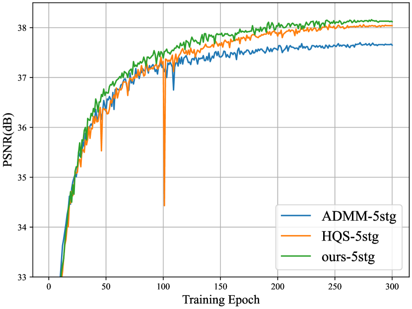
Figure 1: The training PSNR-epoch curve of three unfolding frameworks in 5 stages with CMFormer. Our Residual Adaptive ADMM (R2ADMM) Framework achieves higher PSNR than the others and has a stable training process.

1 Introduction

Hyperspectral images (HSIs) collect and process information from across the electromagnetic spectrum which can better describe the nature of scenes than traditional RGB images. It has a widespread application, such as agriculture Lu et al. (2020), medicine Kado et al. (2018), remote sensing Bioucas-Dias et al. (2013) and object detection Kim et al. (2012); Xu et al. (2015). Therefore, the community pays more attention to the coded aperture snapshot compressive imaging (CASSI) systems Wagadarikar et al. (2008) to improve the sensing speed and reduce the large amount of collected data by compressive sensing 3D signal to 2D sensors. The core of CASSI is to develop a coded aperture mask to modulate the HSI signals (3D) and compress it into the measurement (by 2D sensors). Hence, one major issue is to design a reliable and fast reconstruction algorithm to recover target signals from a 2D compressed image.

To solve the ill-posed inverse problem, classical model-based methods Kittle et al. (2010); Liu et al. (2018b); Yuan (2016) attempt to construct a series of hand-crafted features and regularizations by analyzing the imaging formation. However, the methods need to tune parameters manually and the generalization suffers from model capacity.

End-to-end methods Meng et al. (2020c); Hu et al. (2022); Cai et al. (2022a); Meng et al. (2020b); Cai et al. (2022b) formulate the HSI reconstruction as a regression problem. They can achieve decent reconstruction results by virtue of deep neural networks. However, they ignore the priors and principles of CASSI systems so it’s difficult to adapt to various real scenarios. From this perspective, we hypothesize that it is desirable to inject the priors of the CASSI system into deep neural networks.

Deep Unfolding methods Ma et al. (2019); Huang et al. (2021); Meng et al. (2020a); Wang et al. (2020); Cai et al. (2022c) build a bridge between classical and end-to-end deep learning methods. They combine the priors of the CASSI signal encoding process. The architecture is a multi-stage network, each stage consists of a linear layer and a denoising network (denoiser). The linear layer, where the goal is to formulate the entire reconstruction process as a maximum a posteriori (MAP) optimization problem, and the denoiser, where the goal is to leverage the prior knowledge of images. Given this, we design a simple denoiser and an adaptive optimization algorithm to tap the potential of deep unfolding methods.

Recently, Vision Transformer (ViT) Dosovitskiy et al. (2020); Liu et al. (2021) has achieved great success thanks to its long-range dependencies, less inductive bias, and large capacity. Due to the huge computational burden and over-smoothing issues of ViT, we design a simple convolutional modulation—yet non-attentional—block with a depth-wise feed-forward network to capture the high-frequency signals from 2D measurement.

We present SAUNet, a Simple Adaptive Unfolding Network for HSI reconstruction (Figure 2). While previous HSI methods have used Half-Quadradic Splitting (HQS) and Alternating Direction Method of Multipliers (ADMM) to unfold their networks. We revisit the pros and cons of the two algorithms and observe that original HQS leads to unstable training. Also, directly using ADMM has accuracy degradation issues. Therefore, we introduce a group of learnable parameters to relax the residual term, which stabilizes training and obtains better reconstruction results. In addition, we simplify self-attention design via convolutional modulation operation under the inspiration of FocalNet Yang et al. (2022) and Conv2Former Hou et al. (2022), which makes it possible to earn favorable results at less training time and fast speed (Figure 3). In conclusion, our contributions are as follows:
(1) We propose a novel residual adaptive unfolding framework (R2ADMM) for HSI reconstruction.
(2) We introduce a simple convolutional modulation block (CMB) with a depth-wise feed-forward network into denoiser as CMFormer, for efficient training and inference.
(3) We launch a fair comparison between SAUNet with state-of-the-art algorithms in training time, inference speed, precision, and computational consumption.
(4) We investigate the key factors affecting our network performance and set new records in HSI benchmarks.

2 Related Work

Unfolding Methods for HSI Reconstruction.

Unfolding-based methods usually build the objective function by analyzing the image degradation process from a Bayesian perspective Monga et al. (2021). The iterative learning process can be decomposed into solving the data fidelity term and the regularization term alternately. The data fidelity term can guarantee the solution accord with the degradation process. In most imaging inverse problems, it’s a linear optimization problem that many optimization algorithms including HQS He et al. (2013), ADMM Boyd et al. (2011) and FISTA Beck and Teboulle (2009) can solve. Another term aims to enforce desired property of the output and constraint the solution space with image prior knowledge. Since both the alternate optimized networks are differentiable, the methods enable training end-to-end. GAP-Net Meng et al. (2020a) reconstructs HSI signals by unfolding the generalized alternating projection algorithm and employing trained autoencoder-based denoisers. ADMM-Net Ma et al. (2019) unfolds the ADMM algorithm and designs a DNN based on tensor operations for snapshot compressive imaging. DGSMP Huang et al. (2021) establish an unfolding framework to learn Gaussian Scale Mixture prior. DAUHST Cai et al. (2022c) uses HQS to estimate CASSI degradation patterns to adjust each sub-network. These unfolding methods utilize the sensing matrix to connect traditional iterative algorithms with deep networks.

Convolution Strikes Back

Compared to ViT Dosovitskiy et al. (2020), ConvNets has locality inductive bias, fast training, and easy-to-deploy advantages. Inspired by ViT, several studies revisit the design and training recipe of ConvNets. Ross et al. (2021) further improves the performance of ResNets. ConvNetXt Liu et al. (2022) increases the kernel size up to $7\times 7$ and achieves better performance in vision tasks. RepLKNet Ding et al. (2022) scales up kernels to $31\times 31$ and gives five guides for the design of efficient modern ConvNets. FocalNet Yang et al. (2022) and Conv2former Hou et al. (2022) mimic the Transformer style by designing a convolutional modulation with large kernels. It outperforms several state-of-the-art ConvNets and ViTs in visual recognition tasks.

3 Method

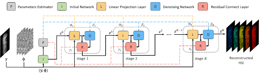
Figure 2: R2ADMM Framework with K stages. ${\boldsymbol{y}}$ and ${\mathbf{\Phi}}$ denote the measurement and sensing matrix respectively. The solid lines indicate the data flow, while the dashed lines indicate the flow of learnable parameters.

3.1 Problem Formulation

In CASSI, let $\boldsymbol{y}\in\mathbb{R}^{t}$ denote the vectorized measurement and $\boldsymbol{n}\in\mathbb{R}^{t}$ signify the vectorized random imaging noise generated by the detector, where $t=H(W+d(N_{\lambda}-1))$. $H$, $W$, $d$, and $N_{\lambda}$ respectively represent the HSI input’s height, width, shifting step in dispersion and the reconstructed number of wavelengths. For the vectorized shifted HSI signal $\boldsymbol{x}\in\mathbb{R}^{tN_{\lambda}}$ and sensing matrix $\mathbf{\Phi}\in\mathbb{R}^{t\times tN_{\lambda}}$ ,which is viewed as shift coded aperture mask. So the degradation model of CASSI can be formed as

$$\boldsymbol{y}=\mathbf{\Phi}\boldsymbol{x}+\boldsymbol{n}.$$ (1)

From a Bayesian perspective, the HSI reconstruction problem can be formulated as solving a MAP problem

$$\hat{\boldsymbol{x}}=\mathop{\arg\min}\limits_{\boldsymbol{x}}\left\|\boldsymbol{y}-\mathbf{\Phi}\boldsymbol{x}\right\|^{2}_{2}+\lambda R(\boldsymbol{x}),$$ (2)

where $\lambda$ is a parameter to balance the data fidelity term and the prior.

3.2 Revisit ADMM and HQS Unfolding

Generally, we solve the problem in Eq.(2) by using an iterative optimization algorithm, such as HQS He et al. (2013), ADMM Boyd et al. (2011). When adopting ADMM to get the unfolding inference, the problem in Eq.(2) converts to solve a constrained optimization problem by introducing an auxiliary variable $\boldsymbol{z}$

$$\small\hat{\boldsymbol{x}}=\mathop{\arg\min}\limits_{\boldsymbol{x}}\left\|\boldsymbol{y}-\mathbf{\Phi}\boldsymbol{x}\right\|^{2}_{2}+\lambda R(\boldsymbol{z}),\quad s.t.\ \boldsymbol{x}=\boldsymbol{z}.$$ (3)

We use the superscript $i$ to index the iteration number and introduce another auxiliary variable $u$. The solution of the problem translates into an iterative solution of the following three subproblems:

$$\small\boldsymbol{x}^{i+1}=\mathop{\arg\min}\limits_{\boldsymbol{x}}\left\|\boldsymbol{y}-\mathbf{\Phi}\boldsymbol{x}\right\|^{2}_{2}+\tau\left\|\boldsymbol{x}-(\boldsymbol{z}^{i}+\boldsymbol{u}^{i})\right\|^{2}_{2}$$ (4)

where $\tau>0$ is a balancing parameter.

$$\small\boldsymbol{z}^{i+1}=\mathop{\arg\min}\limits_{\boldsymbol{z}}\tau\left\|\boldsymbol{z}-(\boldsymbol{x}^{i+1}-\boldsymbol{u}^{i})\right\|^{2}_{2}+\lambda R(\boldsymbol{z})$$ (5)

$$\small\boldsymbol{u}^{i+1}=\boldsymbol{u}^{i}-(\boldsymbol{x}^{i+1}-\boldsymbol{z}^{i+1})$$ (6)

Eq.(4). is a quadratic regularized least-squares problem and it has a closed-form solution:

$$\small\boldsymbol{x}^{i+1}=(\mathbf{\Phi}^{\top}\mathbf{\Phi}+\tau\boldsymbol{I})^{-1}(\mathbf{\Phi}^{\top}\boldsymbol{y}+\boldsymbol{z}^{i}+\boldsymbol{u}^{i})$$ (7)

Notice $\mathbf{\Phi}^{\top}\mathbf{\Phi}\overset{def}{=}diag\{\delta_{1},\delta_{2},...,\delta_{t}\}$ and then simplify the Eq.(7) to make it possible to be solved efficiently via element-wise manipulations instead of huge matrix inversion as

$$\scriptsize\boldsymbol{x}^{i+1}=(\boldsymbol{z}^{i}+\boldsymbol{u}^{i})+\mathbf{\Phi}^{\top}\Big{[}\frac{\boldsymbol{y}_{1}-[\mathbf{\Phi}(\boldsymbol{z}^{i}+\boldsymbol{u}^{i})]_{1}}{\tau+\delta_{1}},...\\ ,\frac{\boldsymbol{y}_{t}-[\mathbf{\Phi}(\boldsymbol{z}^{i}+\boldsymbol{u}^{i})]_{t}}{\tau+\delta_{t}}\Big{]}^{\top}$$ (8)

where $[D]_{k}$ is the $k$-th element in $D$. For the sake of concise expression, we set the parameters $\alpha_{i}=\tau_{i}$, $\boldsymbol{\alpha}=[\alpha_{0},...\alpha_{K}]$ and $\beta=[\tau_{0}/\lambda_{0},...,\tau_{K}/\lambda_{K}]$. So the unfolding framework with ADMM can be reformulated as Algorithm 1, where $I$ signifies the initial network to generate the initial predicted value $\boldsymbol{z}^{0}$ from measurement and mask. $E$ denotes the parameter estimators to control the convergence of each stage of the sub-network like DAUFCai et al. (2022c). $L$ and $R$ is equal to Eq.(8) and Eq.(6) respectively, which represent different linear projection layers. $D$ is a denoiser whose objective function corresponding to is Eq.(5).

The HQS and ADMM unfolding inferences only differ in the derivation of the residual term (Red parts in Algorithm 1). To be Specific, remove the auxiliary variable $u$ from the formula deduction and reserve the rest except the red part in Algorithm 1.

Algorithm 1 ADMM Unfolding Framework for HSI Reconstruction

0:  Measurement: $\boldsymbol{y}$;  Sensing matrix: $\mathbf{\Phi}$

0:  Reconstructed HSI: $\hat{\boldsymbol{x}}$

1:  $\boldsymbol{z}^{0}=I(\boldsymbol{y},\mathbf{\Phi});\ \boldsymbol{\alpha},\boldsymbol{\beta}=E(\boldsymbol{z}^{0});\ {\color[rgb]{1,0,0}\boldsymbol{u^{0}}=0}$(Initial Network)

2:  for $i=0,1,2,...M$  do

3:     $\boldsymbol{x}^{i+1}=L(\boldsymbol{y},\boldsymbol{z}^{i},{\color[rgb]{1,0,0}\boldsymbol{u}^{i}},\alpha_{i},\mathbf{\Phi})$(Linear Projection Layer)

4:     $\boldsymbol{z}^{i+1}=D(\boldsymbol{x}^{i+1},{\color[rgb]{1,0,0}\boldsymbol{u}^{i}},\beta_{i})$(Denoising Network)

5:     $\boldsymbol{u}^{i+1}=\boldsymbol{u}^{i}-(\boldsymbol{x}^{i+1}-\boldsymbol{z}^{i+1})$(Residual Connect Layer)

6:  end for

7:  $\hat{\boldsymbol{x}}\leftarrow\boldsymbol{z}^{i+1}$

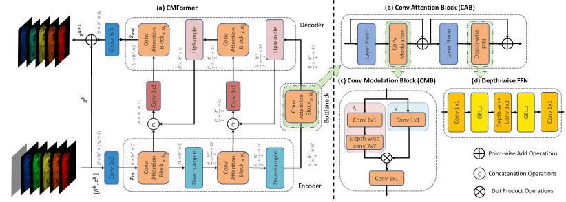
Figure 3: Diagram of CMFormer. (a) CMFormer adopts a U-shaped structure. (b) CAB consists of a depth-wise FFN, a CMB, and two-layer normalization. (c) The structure of CMB. (d) The components of depth-wise FFN.

3.3 Residual Adaptive ADMM Unfolding Framwork

A natural approach to leverage ADMM instead of HQS to unfold the network is that ADMM shows faster convergence and lower error value than HQSLiu et al. (2018a). Also, HQS does not have convergence guarantees for arbitrary convex problems Heide et al. (2016). We directly implement ADMM unfolding framework architecture into 5 stages with the CMFormer as HQS unfolding framework for HSI reconstruction in order to explore the performance difference. As shown in Figure 1, We discover HQS unfolding framework can achieve a better result but converges more slowly than ADMM unfolding framework and has bad training stability, while ADMM’s is the opposite. We hypothesize that HQS unfolding framework extracts more information from the input data to estimate the degradation patterns and ill-posedness degree with a strong denoiser plugging into. However, ADMM unfolding framework constrains between linear project and denoiser strictly in each stage via a residual term, resulting in quick convergence but a lack of adaptive per-stage optimization ability through input.

Thus, we introduce a group of learnable parameters $\mathbf{\gamma}$ to relax residual term. Specifically, we initialize $\mathbf{\gamma}$ to zero to stabilize training. The residual solution process in Algorithm 1 is rewritten as Eq.(9)

$$\small\boldsymbol{u}^{i+1}=\boldsymbol{u}^{i}-\gamma_{i+1}(\boldsymbol{x}^{i+1}-\boldsymbol{z}^{i+1}).$$ (9)

We introduce the R2ADMM framework in Figure 2. Following DAUF Cai et al. (2022c), the initial network $I$ consists of a conv$1\times 1$. The parameters estimator $E$ consists of a conv$1\times 1$, a conv$3\times 3$, a global average pooling, and three fully connected layers. R2ADMM with the help of $E$, can restore the HSI signal from measurement by exploiting mask-modulation and dispersion process information into adaptive variables.

3.4 CMFormer

Recent works applying Transformer for HSI reconstruction make great progress, which is due to Transformer excelling at modeling long-range dependencies. Large kernel convolutions also achieve that with less computational burden. So we propose CMFormer with large kernel convolutional modulation blocks to play the role of denoiser.

Denoiser Network.

The overall architecture of denoiser is shown in Figure 3(a), which is a three-level U-Net Ronneberger et al. (2015) structure with convolutional modulation block. Following HST Cai et al. (2022a), we use a conv$3\times 3$ to map $z_{k}$ concatenated with $\beta_{k}$ into $z_{in}$, whose dimension is $H\times(W+d(N_{\lambda}-1))\times C$. And then $z_{in}$ pass through the encoder, bottleneck, and decoder. Each stage of the encoder and decoder is comprised of convolutional attentional blocks and a resizing module. Each stage, as shown in Figure 3(b), consists of two-layer normalization (LN), Convolutional Modulation block (CMB), and a depth-wise Feed-Forward Network (FFN, Figure 3(d)). The downsampling layer of the encoder and upsampling layer of the decoder is strided conv$4\times 4$ and deconv$2\times 2$. Finally, conv$3\times 3$ operates the output of the decoder $z_{out}$ in the wake of point-wise add operation with $z_{k}$, we get the output $z_{k+1}$ of the denoiser.

In the implementation, we set each stage of block number $[N_{1},N_{2},N_{3}]$ as $[1,1,3]$ in order to balance the computation costs and reconstruction performance.

Algorithms	Params	GFLOPs	S1	S2	S3	S4	S5	S6	S7	S8	S9	S10	Avg
TSA-Net Meng et al. (2020b)	44.25M	110.06	32.03 0.892	31.00 0.858	32.25 0.915	39.19 0.953	29.39 0.884	31.44 0.908	30.32 0.878	29.35 0.888	30.01 0.890	29.59 0.874	31.46 0.874
HDNet Hu et al. (2022)	2.37M	157.76	35.14 0.935	35.67 0.940	36.03 0.943	42.30 0.969	32.69 0.946	34.46 0.952	33.67 0.926	32.48 0.941	34.89 0.942	32.38 0.937	34.97 0.943
MST-S Cai et al. (2022a)	0.93M	12.96	34.71 0.930	34.45 0.925	35.32 0.943	41.50 0.967	31.90 0.933	33.85 0.943	32.69 0.911	31.69 0.933	34.67 0.939	31.82 0.926	34.26 0.935
MST-L Cai et al. (2022a)	2.03M	28.15	35.40 0.941	35.87 0.944	36.51 0.953	42.27 0.973	32.77 0.947	34.80 0.955	33.66 0.925	32.67 0.948	35.39 0.949	32.50 0.941	35.18 0.948
CST-S Cai et al. (2022b)	1.20M	11.67	34.78 0.930	34.81 0.931	35.42 0.944	41.84 0.967	32.29 0.939	34.49 0.949	33.47 0.922	32.89 0.945	34.96 0.944	32.14 0.932	34.71 0.940
CST-L Cai et al. (2022b)	3.00M	27.81	35.82 0.947	36.54 0.952	37.39 0.959	42.28 0.972	33.40 0.953	35.52 0.962	34.44 0.937	33.83 0.959	35.92 0.951	33.36 0.948	35.85 0.954
CST-L*Cai et al. (2022b)	3.00M	40.10	35.96 0.949	36.84 0.955	38.16 0.962	42.44 0.975	33.25 0.955	35.72 0.963	34.86 0.944	34.34 0.961	36.51 0.957	33.09 0.945	36.12 0.957
Methods based on deep unfolding algorithm follow:
DGSMP Huang et al. (2021)	3.76M	646.65	33.26 0.915	32.09 0.898	33.06 0.925	40.54 0.964	28.86 0.882	33.08 0.937	30.74 0.886	31.55 0.923	31.66 0.911	31.44 0.925	32.63 0.917
GAP-Net Meng et al. (2020a)	4.27M	78.58	33.74 0.911	33.26 0.900	34.28 0.929	41.03 0.967	31.44 0.919	32.40 0.925	32.27 0.902	30.46 0.905	33.51 0.915	30.24 0.895	33.26 0.917
ADMM-Net Ma et al. (2019)	4.27M	78.58	34.12 0.918	33.62 0.902	35.04 0.931	41.15 0.966	31.82 0.922	32.54 0.924	32.42 0.896	30.74 0.907	33.75 0.915	30.68 0.895	33.58 0.918
DAUHST-2stg Cai et al. (2022c)	1.40M	18.44	35.93 0.943	36.70 0.946	37.96 0.959	44.38 0.978	34.13 0.954	35.43 0.957	34.78 0.940	33.65 0.950	37.42 0.955	33.07 0.941	36.34 0.952
DAUHST-3stg Cai et al. (2022c)	2.08M	27.17	36.59 0.949	37.93 0.958	39.32 0.964	44.77 0.980	34.82 0.961	36.19 0.963	36.02 0.950	34.28 0.956	38.54 0.963	33.67 0.947	37.21 0.959
DAUHST-5stg Cai et al. (2022c)	3.44M	44.61	36.92 0.955	38.52 0.962	40.51 0.967	45.09 0.980	35.33 0.964	36.56 0.965	36.82 0.958	34.74 0.959	38.71 0.963	34.27 0.952	37.75 0.962
DAUHST-9stg Cai et al. (2022c)	6.15M	79.50	37.25 0.958	39.02 0.967	41.05 0.971	46.15 0.983	35.80 0.969	37.08 0.970	37.57 0.963	35.10 0.966	40.02 0.970	34.59 0.956	38.36 0.967
SAUNet-1stg	0.78M	9.52	34.66 0.936	34.78 0.933	36.74 0.955	43.33 0.979	32.14 0.941	34.28 0.952	33.29 0.927	32.18 0.947	35.24 0.950	31.79 0.936	34.84 0.946
SAUNet-2stg	1.50M	17.91	36.25 0.951	37.13 0.956	38.95 0.968	44.61 0.984	34.23 0.961	35.66 0.964	35.33 0.948	33.84 0.961	38.13 0.964	33.14 0.950	36.73 0.961
SAUNet-3stg	2.23M	26.31	36.67 0.957	38.21 0.964	40.76 0.975	45.86 0.988	34.57 0.964	36.16 0.970	36.18 0.956	33.92 0.965	39.54 0.973	33.54 0.955	37.54 0.966
SAUNet-5stg	3.68M	43.10	37.14 0.961	39.05 0.970	41.27 0.975	46.90 0.990	34.91 0.969	36.52 0.973	36.86 0.961	34.81 0.969	40.05 0.975	34.05 0.960	38.16 0.970
SAUNet-9stg	6.59M	76.68	37.15 0.964	39.86 0.975	42.14 0.979	46.71 0.991	36.08 0.973	37.01 0.974	37.28 0.965	34.64 0.971	40.45 0.976	34.38 0.963	38.57 0.973
SAUNet-13stg	9.50M	110.25	37.37 0.964	40.31 0.977	42.67 0.980	47.33 0.991	35.62 0.973	36.96 0.975	37.42 0.966	35.20 0.973	40.73 0.977	34.35 0.964	38.79 0.974

Table 1: Comparisons between SAUNet and SOTA methods on 10 simulation scenes (S1$\sim$S10). Params, FLOPS, PSNR (upper entry in each cell), and SSIM (lower entry in each cell) are reported.

Convolutional Modulation Block.

In each CMB, instead of obtaining similarity score matrix $\mathbf{A}$ via key matrix $\mathbf{K}$ and query matrix $\mathbf{Q}$ like Transformer. We directly compute $\mathbf{A}$ and modulate the value matrix $\mathbf{V}$ in Figure 3(c). Specifically, for a input $\mathbf{X}\in\mathbb{R}^{H\times W\times C}$the operations we apply as follows:

$$\small\mathbf{A}=\mathrm{DWConv}_{k\times k}(\mathbf{W_{1}X})$$ (10)

$$\small\mathbf{V}=\mathbf{W_{2}X}$$ (11)

$$\small\mathbf{Output}=\mathbf{W_{3}(A\odot V)}$$ (12)

where $\mathbf{W_{1}}$,$\mathbf{W_{2}}$,$\mathbf{W_{3}}$ are weights of linear layers which are implemented by conv$1\times 1$. $\odot$ is a the Hadamard product. $\mathrm{DSConv}$ represents depth-wise convolution with kernel size $k\times k$. In this work, we select depth-wise conv$7\times 7$ after trading off computation overhead, speed, and accuracy.

Model	TSA-Net	DGSMP	GAP-Net	ADMM-Net	MST-S	MST-L	HDNet	CST-S	CST-L	CST-L*	DAUHST-2stg	DAUHST-3stg	DAUHST-5stg	DAUHST-9stg	SAUNet-1stg	SAUNet-2stg	SAUNet-3stg	SAUNet-5stg	SAUNet-9stg	SAUNet-13stg
Training Hours	28.5	148.4	48.8	48.8	48.6	119.9	34.7	17.5	43.6	58.1	40.9	61.5	102.6	216.9	14.3	29.3	43.9	71.5	149.0	214.98
Inference FPS	32.8	8.0	19.0	18.6	23.2	8.6	44.8	45.3	16.1	14.8	31.0	21.9	13.3	7.5	56.4	31.5	22.0	13.1	7.8	5.5

Table 2: Comparisons between SAUNet and 8 SOTA methods with their variants in training GPU hours and inference speed at a Tesla v100 GPU. We record the forward and backward time of each model training in a GPU for 300 epochs at batch-size=5 as training hours.

4 Experiment

4.1 Experiment Settings

We follow TSA-Net Meng et al. (2020b) to adopt 28 wavelengths from 450nm to 650nm derived by spectral interpolation for simulation and real HSI reconstruction experiments.

Datasets.

For Synthetic experiments, we conduct simulations on two public datasets, CAVE Yasuma et al. (2010) and KAIST Choi et al. (2017). For a fair comparison, we use the mask at a size of $256\times 256$ as the same as TSA-Net Meng et al. (2020b). We select 10 scenes from KAIST for testing and the others are used for training. For real HSI restoration experiments, we use the real data developed in Meng et al. (2020b).

Evaluation Metrics.

For simulation experiments, we adopt PSNR and SSIM for quantitative comparison. For the real data experiments, we select the Naturalness Image Quality Evaluator (NIQE) Mittal et al. (2012), a no-reference image quality assessment metric in the absence of ground truth.

Implementation Details.

We implement our model in Pytorch. All models are trained with Adam optimizer ($\beta_{1}=0.9$ and $\beta_{2}=0.999$) for 300 epochs with the Cosine Annealing scheduler. The initial learning rate is $4\times 10^{-4}$. We randomly crop patches with the spatial size of $256\times 256$ and $660\times 660$ from 3D HSI cubes as training samples for simulation and real experiments. Following TSA-Net Meng et al. (2020b), the shifting step $d$ in dispersion is set to 2 and the batch size is 5. We set reconstructed channel $C=N_{\lambda}=28$. Data augmentation is made of random flipping and rotation. The training cost function is to minimize the $l1$ loss between the reconstructed HSIs and ground truth.

4.2 Simulation HSI Reconstruction.

Table 1 compares the Params, FLOPs, PSNR and SSIM of SAUNet, and 8 SOTA methods with their variations. For fair comparisons, all methods are tested with the same setting as DAUHST. SAUNet surpasses DAUHST in both GFLOPs and PSNR/SSIM for each unfolding stage. Moreover, SAUNet could easily scale up to 13 stage to get better performance without training divergence. Without bells and whistles, SAUNet set new state-of-the-art in the simulation dataset. Table 2 compares training time and test inference FPS of SAUNet and 8 SOTA methods in a Tesla V100 GPU. We re-train all models for 300 epochs with the toolbox of MST Cai et al. (2022a) at 5 batch size. For DAUHST-9stg and SAUNet-9stg models, the original training scheme with 5 batch size results that the training process is interrupted on account of insufficient memory, and thus we adopt gradient checkpointing Chen et al. (2016) technology in each denoiser’s encoder, decoder, and bottleneck. It shows SAUNet has less training time while faster inference speed compared to other unfolding counterparts. Figure 4 depicts the simulation HSI reconstruction comparisons between our DAUHST and other SOTA methods on Scene 5 with 4 (out of 28) spectral channels. SAUNet has more similar spectral density curves than other methods.

4.3 Real HSI Reconstruction

We further evaluate the effectiveness of our approach, SAUNet, in real HSI reconstruction. For a fair comparison, we re-train SAUNet-3stg from scratch with the real mask on the CAVE and KAIST datasets jointly as the same as MST Cai et al. (2022a). To simulate the real imaging situations, 11-bit shot noise is injected during training. Without ground truth for comparison, we quantitatively evaluate the 4 SOTA methods and our SAUNet-3stg with NIQE in Table 3. Figure 5 shows reconstructed images of Scene 3 with 4 of 28 spectral channels between our SAUNet methods and 6 SOTA methods. It shows SAUNet can reconstruct HSIs with cleaner textures, and fewer artifacts in all wavelengths.

Model	HDNet	MST	CST	DAUHST-3stg	ours-3stg
NIQE$\downarrow$	5.8689	6.8155	6.5245	5.5000	5.1961

Table 3: Naturalness Image Quality Evaluator (NIQE) evaluation on real dataset. 4 SOTA methods and SAUNet-3stg are included.

Baseline	CMB	R2ADMM	PSNR	SSIM	params (M)	GFLOPs
✓			35.51	0.954	1.69	19.94
✓	✓		35.77	0.957	2.18	25.25
✓		✓	36.74	0.961	1.74	21.00
✓	✓	✓	37.54	0.966	2.23	26.31

((a))

denoiser	algorithms	PSNR	SSIM	params (M)	GFLOPs
CMFormer	w/o	35.77	0.957	2.18	25.25
CMFormer	HQS	37.40	0.966	2.23	26.31
CMFormer	ADMM	37.43	0.965	2.23	26.31
CMFormer	ours	37.54	0.966	2.23	26.31
w/o CAB	w/o	23.13	0.559	0.54	8.22
w/o CAB	HQS	29.77	0.736	0.59	9.28
w/o CAB	ADMM	30.13	0.747	0.59	9.28
w/o CAB	ours	30.21	0.751	0.59	9.28

((b))

kernel size	PSNR	SSIM	params (M)	GFLOPs
$3\times 3$	34.34	0.941	0.76	9.17
$5\times 5$	34.54	0.943	0.76	9.31
$7\times 7$	34.84	0.946	0.78	9.52
$11\times 11$	35.12	0.949	0.81	10.14
$13\times 13$	35.11	0.948	0.84	10.55

((c))

FFN	PSNR	SSIM	params (M)	GFLOPs
ours-1stg	34.84	0.946	0.78	9.52
w/o	33.67	0.928	0.39	5.61
w/o dw conv	34.41	0.942	0.76	9.21
$1\times 1$ conv	34.36	0.941	1.48	16.40

((d))

Table 4: Ablation studies on simulation datasets. PSNR, SSIM, Params, and FLOPs are reported.

4.4 Ablation Study

Break-down Ablation.

We conduct a break-down ablation experiment to investigate the effect of each component towards higher performance. The results are listed in Table 4(a). The baseline that is derived by removing CMB and R2ADMM from SAUNet-3stg yields 35.51 dB. When we respectively apply CMB and R2ADMM, the model achieves 0.26 dB and 1.23 dB improvements. When we employ CMB and R2ADMM jointly, the model gains by 2.03 dB. These results demonstrate the effectiveness of CMB and R2ADMM.

Unfolding Framework.

We compare R2ADMM with different algorithm unfolding frameworks, including ADMM and HQS. In particular, HQS-based deep unfolding framework is DAUF in essence. We report results in Table 4(b). Our results surpass the direct stack structure of a network with CMFormer and a bad denoiser, which removes all CABs from CMFormer, by 1.77 dB and 7.08 dB. It indicates the importance of deep unfolding framework for HSI reconstruction. Moreover, R2ADMM outperforms HQS and ADMM unfolding framework by 0.44 dB and 0.08 dB in a bad denoiser while 0.14 dB and 0.11 dB in CMFormer, which demonstrate the good generalization performance of R2ADMM.

Kernel Size in CMB.

The kernel size is a significant factor to influence the model reconstruction performance. We select 5 different kernels size, i.e., $\{3\times 3,5\times 5,7\times 7,11\times 11,13\times 13\}$ to carry out our experiments in SAUNet-1stg. As shown in Table 4(c), the gains seem to saturate until the kernel size is increased up to $13\times 13$. This may be due to excessively large receptive fields having little effect on the reconstruction task. In default, we use the kernel size of $7\times 7$.

Depth-wise FFN Structure.

In this part, we reveal the importance of the neglected FFN structure. Our experiments are based on SAUNet-1stg and the results can be found in Table 4(d). When we remove the whole FFN, depth-wise conv$3\times 3$ and replace depth-wise conv with conv$1\times 1$, the results of PSNR are lost by 1.17dB, 0.43 dB, and 0.48 dB, even though the replacement of conv$1\times 1$ increases the amount of 6.88 GFLOPs computation. We hypothesize that FFN introduces more nonlinear properties to increase the representation ability, while the structure of CMB tends to smooth features with large kernel size Park and Kim (2022).

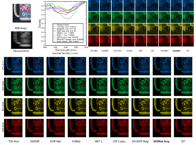
Figure 4: Reconstructed simulation HSI comparisons of Scene 5 with 4 out of 28 spectral channels. The top-middle shows the spectral curves corresponding to the red box of the RGB image. The top-right depicts the enlarged patches corresponding to the red boxes in the bottom HSIs. Zoom in for a better view.

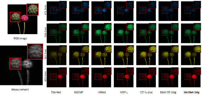
Figure 5: Real HSI reconstruction comparison of Scene 3. 4 out of 28 spectra are randomly selected. Zoom in for a better view.

5 Conclusion

In this work, we present SAUNet, a simple and efficient deep unfolding network for HSI reconstruction. It consists of a deep unfolding framework, R2ADMM, and U-Net architecture denoisers with Convolutional Modulation Block, CMFormer. R2ADMM adapts to each restoring subnetwork via relaxing each residual term from data, while CMFormer introduces convolutional modulation with large convolutional kernels to simplify the structure and reduce the computation burden. Therefore, SAUNet can achieve reconstruction performance with less training time and fast inference speed. Moreover, we investigate the effect of each component towards higher performance and point out that the design of ignoring Depth-wise FFN has an important influence the same as others. In the future, we will delve into the robustness and generalization of the reconstruction algorithm in real scenes.

Appendix

The technical appendix is organized as follows:

• Section A: mathematical model of CASSI.

• Section B: the detailed derivation of the unfolding framework with Half-Quadradic Splitting (HQS) and Alternating Direction Method of Multipliers (ADMM).

• Section C: more quantitative comparisons.

• Section D: more qualitative comparisons.

• Section E: hyperparameter details.

• Section F: more ablation studies of our Residual adaptive Unfolding framework (R2ADMM), Convolutional Attention Block (CAB) and SAUNet.

• Section G: limitations.

• Section H: broader impact.

Appendix A Mathematical Model of CASSI

In a CASSA system (Figure 6), we denote the 3D HSI data cube as $\boldsymbol{F}\in\mathbb{R}^{H\times W\times N_{\lambda}}$, where $H$, $W$, and $N_{\lambda}$ are the HSI input’s height, width and the number of reconstructed wavelengths. First, a pre-defined coded aperture mask $\boldsymbol{M}^{*}\in\mathbb{R}^{H\times W}$ is used to modulate $\boldsymbol{F}$ along the spectral dimension as:

$$\boldsymbol{F}^{\prime}(:,:,n_{\lambda})=\boldsymbol{F}(:,:,n_{\lambda})\odot\boldsymbol{M}^{*}$$ (13)

where $n_{\lambda}\in[1,...,N_{\lambda}]$ indexes the spectral wavelengths, and $\odot$ is the element-wise multiplication.

Then input the modulated HSI signal $\boldsymbol{F}^{\prime}$ to a disperser. During the process, $\boldsymbol{F}$ is tilted and sheared along the dimension of width. Let us use $\boldsymbol{F}^{\prime\prime}\in\mathbb{R}^{H\times(W+d(N_{\lambda}-1))\times N_{\lambda}}$ to be noted the tilted cube, and we have

$$\boldsymbol{F}^{\prime\prime}(u,v,n_{\lambda})=\boldsymbol{F}^{\prime}(x,y+d({\lambda}_{n}-{\lambda}_{c}),n_{\lambda})$$ (14)

where $(u,v)$ is the position on the coordinate system of the detector plane, $\lambda_{n}$ is the wavelength of the $n_{\lambda}$-th spectral channel, and $\lambda_{c}$ is the base wavelength which means it does not shift after passing a disperser. $d$ is the shifting step.

Finally, the 2D measurement $\boldsymbol{Y}\in\mathbb{R}^{H\times(W+d(N_{\lambda}-1))}$ by integrating all signals of the spectral channel:

$$\boldsymbol{Y}=\sum_{n_{\lambda}=1}^{N_{\lambda}}\boldsymbol{F}^{\prime\prime}(:,:,n_{\lambda})+\boldsymbol{G}$$ (15)

where $\boldsymbol{G}\in\mathbb{R}^{H\times(W+d(N_{\lambda}-1))}$ signifies the random imaging noise generated by the detector.

To simply the above description, we denote the $\boldsymbol{M}\in\mathbb{R}^{H\times(W+d(N_{\lambda}-1))\times N_{\lambda}}$ and $\boldsymbol{\hat{F}}\in\mathbb{R}^{H\times(W+d(N_{\lambda}-1))\times N_{\lambda}}$ as the shifted version of mask $\boldsymbol{M}^{*}$ and 3D HSI cube $\boldsymbol{F}$. Their relationship is as follows:

$$\boldsymbol{M}(u,v,n_{\lambda})=\boldsymbol{M}^{*}(x,y+d(\lambda_{n}-\lambda_{c}))$$ (16)

$$\boldsymbol{\hat{F}}(u,v,n_{\lambda})=\boldsymbol{F}(x,y+d(\lambda_{n}-\lambda_{c}),n_{\lambda})$$ (17)

We can reformulated Eq.(15) as

$$\boldsymbol{Y}=\sum_{n_{\lambda}=1}^{N_{\lambda}}\boldsymbol{\hat{F}}(:,:,n_{\lambda})\odot\boldsymbol{M}(:,:,n_{\lambda})+\boldsymbol{G}$$ (18)

Vectorization.

Let $\mathrm{vec}(\cdot)$ represent the matrix vectorization, i.e., concatenates all the columns of a matrix as a single vector. Define $\boldsymbol{y}=\mathrm{vec}(\boldsymbol{Y})\in\mathbb{R}^{t}$ and $\boldsymbol{n}=\mathrm{vec}(\boldsymbol{N})\in\mathbb{R}^{t}$, where $t=H(W+d(N_{\lambda}-1))$. As for original 3D HSI cube, we denote the $\boldsymbol{x}_{n_{\lambda}}=\mathrm{vec}(\boldsymbol{\hat{F}}(:,:,n_{\lambda}))$. So the vector $\boldsymbol{x}$ is

$$\boldsymbol{x}=\mathrm{vec}([\boldsymbol{x}_{1},\boldsymbol{x}_{2},...,\boldsymbol{x}_{N_{\lambda}}])\in\mathbb{R}^{t\times{N_{\lambda}}}.$$ (19)

Similar to above steps, we denote the sensing matrix $\mathbf{\Phi}\in R^{t\times tN_{\lambda}}$ as

$$\mathbf{\Phi}=[\mathbf{\Phi}_{1},\mathbf{\Phi}_{2},...,\mathbf{\Phi}_{N_{\lambda}}],$$ (20)

where the $\mathbf{\Phi}=\mathrm{diag}(\mathrm{vec}(\mathrm{\boldsymbol{M}(:,:,n_{\lambda})))}$ So the vectorized version of Eq.(18) is

$$\boldsymbol{y}=\mathbf{\Phi}\boldsymbol{x}+\boldsymbol{n}.$$ (21)

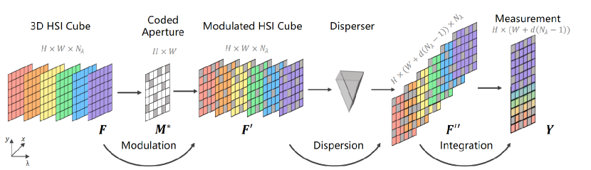
Figure 6: Illustration of a Single Disperser Coded Aperture Snapshot Spectral Imaging (SD-CASSI) system.

Eq.(21) is the sensing matrix and is similar to compressive sensing due to the number of columns more than rows. Nevertheless, because of the special structure of Eq.(20) for $\mathbf{\Phi}$, we can not directly use compressive sensing theories in HSI reconstructions. Fortunately, it has been proved that the signal can be reconstructed even when $N_{\lambda}>1$.

Our work is based on the pre-designed CASSI system, which is given measurement $\boldsymbol{y}$ and sensing matrix $\mathbf{\Phi}$ to recover the original HSI cube $\boldsymbol{x}$. It is also the one of major tasks in CASSI.

Appendix B Detailed derivation of HQS and ADMM

DAUHST Cai et al. (2022c) has applied the HQS optimization algorithm to the unfolding framework for HSI reconstruction. The method is shown as Algorithm 2. In this section, we give the detailed derivation of the ADMM algorithm for HSI reconstruction.

Algorithm 2 HQS Unfolding Framework (DAUHST) for HSI Reconstruction

0:  Measurement: $\boldsymbol{y}$;  Sensing matrix: $\mathbf{\Phi}$

0:  Reconstructed HSI: $\hat{\boldsymbol{x}}$

1:  $\boldsymbol{z}^{0}=I(\boldsymbol{y},\mathbf{\Phi});\ \boldsymbol{\alpha},\boldsymbol{\beta}=E(\boldsymbol{z}^{0});$(Initial Network)

2:  for $i=0,1,2,...M$  do

3:     $\boldsymbol{x}^{i+1}=L(\boldsymbol{y},\boldsymbol{z}^{i},\alpha_{i},\mathbf{\Phi})$(Linear Projection Layer)

4:     $\boldsymbol{z}^{i+1}=D(\boldsymbol{x}^{i+1},\beta_{i})$(Denoising Network)

5:  end for

6:  $\hat{\boldsymbol{x}}\leftarrow\boldsymbol{z}^{i+1}$

For Eq.(21), we take a Bayesian perspective to translate the problem of solving x into an optimization problem as follows:

$$\hat{\boldsymbol{x}}=\mathop{\arg\min}\limits_{\boldsymbol{x}}\left\|\boldsymbol{y}-\mathbf{\Phi}\boldsymbol{x}\right\|^{2}_{2}+\lambda R(\boldsymbol{x}),$$ (22)

where $\left\|\boldsymbol{y}-\mathbf{\Phi}\boldsymbol{x}\right\|^{2}_{2}$ is the data fidelity term, $R(\boldsymbol{x})$ is the regularization term, which is related to the image prior. And the $\lambda$ is a hyperparameter to balance the two above terms.

The ADMM is adopted to decouple the data fidelity term and the regularization term in Eq.(22). By introducing an auxiliary variable $z$, the Eq.(22) can be written in the equivalent form:

$$\hat{\boldsymbol{x}}=\mathop{\arg\min}\limits_{\boldsymbol{x}}\left\|\boldsymbol{y}-\mathbf{\Phi}\boldsymbol{x}\right\|^{2}_{2}+\lambda R(\boldsymbol{z}),\quad s.t.\ \boldsymbol{x}=\boldsymbol{z}.$$ (23)

Next, we give the associated augmented Lagrangian function as

$$\mathcal{L}_{\tau}(\boldsymbol{x},\boldsymbol{z},\boldsymbol{v})=\left\|\boldsymbol{y}-\mathbf{\Phi}\boldsymbol{x}\right\|^{2}_{2}+\lambda R(\boldsymbol{z})+$$ (24)

$$\boldsymbol{v}^{\top}(\boldsymbol{x}-\boldsymbol{z})+\rho\left\|\boldsymbol{x}-\boldsymbol{z}\right\|^{2}_{2},$$

with $\boldsymbol{v}$ the dual variable, and $\tau>0$ the penalty parameter. Scaling $\boldsymbol{v}$ as $\boldsymbol{u}=\frac{1}{\tau}\boldsymbol{y}$, the Eq.(24) can be iteratively solved by repeating the following successive steps:

$$\boldsymbol{x}^{i+1}=\mathop{\arg\min}\limits_{\boldsymbol{x}}\left\|\boldsymbol{y}-\mathbf{\Phi}\boldsymbol{x}\right\|^{2}_{2}+\tau^{i}\left\|\boldsymbol{x}-(\boldsymbol{z}^{i}+\boldsymbol{u}^{i})\right\|^{2}_{2},$$ (25)

$$\boldsymbol{z}^{i+1}=\mathop{\arg\min}\limits_{\boldsymbol{z}}\tau^{i}\left\|\boldsymbol{z}-(\boldsymbol{x}^{i+1}-\boldsymbol{u}^{i})\right\|^{2}_{2}+\lambda R(\boldsymbol{z}),$$ (26)

$$\boldsymbol{u}^{i+1}=\boldsymbol{u}^{i}-(\boldsymbol{x}^{i+1}-\boldsymbol{z}^{i+1}),$$ (27)

where $\tau^{i}$ denotes the penalty parameter at the $i$-th iteration. Eq.(25) is a quadratic regularized least-squares problem and we take the derivative versus $x$ of Eq.(25) to get the closed-form solution:

$$\boldsymbol{x}^{i+1}=(\mathbf{\Phi}^{\top}\mathbf{\Phi}+\tau\boldsymbol{I})^{-1}(\mathbf{\Phi}^{\top}\boldsymbol{y}+\boldsymbol{z}^{i}+\boldsymbol{u}^{i}).$$ (28)

Notice $\mathbf{\Phi}^{\top}\mathbf{\Phi}\overset{def}{=}diag\{\delta_{1},\delta_{2},...,\delta_{t}\}$ from Section A, where $\delta_{k}$ is equal to the $k$-th element squared of $\mathrm{vec}(M^{*})$. We continue to simpify Eq.(28), we can get the results:

$$\boldsymbol{x}^{i+1}=(\boldsymbol{z}^{i}+\boldsymbol{u}^{i})+\mathbf{\Phi}^{\top}\Big{[}\frac{\boldsymbol{y}_{1}-[\mathbf{\Phi}(\boldsymbol{z}^{i}+\boldsymbol{u}^{i})]_{1}}{\tau+\delta_{1}},...$$ (29)

$$,\frac{\boldsymbol{y}_{t}-[\mathbf{\Phi}(\boldsymbol{z}^{i}+\boldsymbol{u}^{i})]_{t}}{\tau+\delta_{t}}\Big{]}^{\top}.$$

For the sake of concise expression, we set the parameters $\alpha_{i}=\tau_{i}$, $\boldsymbol{\alpha}=[\alpha_{0},...\alpha_{K}]$ and $\beta=[\tau_{0}/\lambda_{0},...,\tau_{K}/\lambda_{K}]$. We can get the unfolding framework with ADMM.

However, ADMM requires that $R(\boldsymbol{x})$ is a closed, proper, convex function. And the deep learning denoiser tends not to meet the condition. Therefore, some work from a good denoiser designer Qiao et al. (2020); Ma et al. (2019) or improve ADMM Xu et al. (2016, 2017); Liu et al. (2019) in order to adapt to the problem.

Appendix C More Quantitative Comparisons

Algorithms	PSNR	SSIM	Params	GFLOPs	Training Hours	Inference FPS
TwIST Bioucas-Dias and Figueiredo (2007)	23.12	0.669	-	-	-	-
GAP-TV Yuan (2016)	24.36	0.669	-	-	-	-
DeSCI Liu et al. (2018b)	25.27	0.721	-	-	-	-
$\lambda$-Net Miao et al. (2019)	28.53	0.841	62.64M	117.98	9.43	127.14
TSA-Net Meng et al. (2020b)	31.46	0.894	44.25M	110.06	28.54	32.83
DGSMP Huang et al. (2021)	32.63	0.917	3.76M	646.65	148.44	7.98
GAP-Net Meng et al. (2020a)	33.26	0.917	4.27M	78.58	48.81	19.00
ADMM-Net Ma et al. (2019)	33.58	0.918	4.27M	78.58	48.82	18.63
HDNet Hu et al. (2022)	34.97	0.943	2.37M	154.76	34.71	44.75
MST-S Cai et al. (2022a)	34.26	0.935	0.93M	12.96	48.63	23.17
MST-M Cai et al. (2022a)	34.94	0.943	1.50M	18.07	67.66	14.33
MST-L Cai et al. (2022a)	35.18	0.948	2.03M	28.15	119.89	8.61
CST-S Cai et al. (2022b)	34.71	0.940	1.20M	11.67	17.54	45.27
CST-M Cai et al. (2022b)	35.31	0.947	1.36M	16.91	30.38	26.77
CST-L Cai et al. (2022b)	35.85	0.954	3.00M	27.81	43.55	16.14
CST-L∗ Cai et al. (2022b)	36.12	0.957	3.00M	40.10	58.11	14.82
BIRNAT Cheng et al. (2022)	37.58	0.948	4.40M	2122.66	263.61	1.49
DAUHST-2stg Cai et al. (2022c)	36.34	0.952	1.40M	18.44	40.92	30.98
DAUHST-3stg Cai et al. (2022c)	37.21	0.959	2.08M	27.17	61.49	21.87
DAUHST-5stg Cai et al. (2022c)	37.75	0.962	3.44M	44.61	102.59	13.29
DAUHST-9stg Cai et al. (2022c)	38.36	0.967	6.15M	79.50	216.89	7.53
SAUNet-1stg	34.84	0.946	0.78M	9.52	14.25	56.43
SAUNet-2stg	36.73	0.961	1.50M	17.91	29.28	31.52
SAUNet-3stg	37.54	0.966	2.23M	26.31	43.92	22.05
SAUNet-5stg	38.16	0.970	3.68M	43.10	71.45	13.31
SAUNet-9stg	38.57	0.973	6.59M	76.68	148.96	7.67
SAUNet-13stg	38.79	0.974	9.50M	110.25	214.98	5.46

Table 5: Comparisons between SAUNet and other SOTA methods with their variants in average PSNR, SSIM of 10 scenes, Params, GFLOPs training GPU hours and inference speed at a Tesla v100 GPU. We record the forward and backward time of each model training in a GPU for 300 epochs at batch-size=5 as training hours.

In this section, we will give more PSNR, SSIM, Params, GFLOPs, training GPU time and inference FPS of SOTA models at Table 5. The experiments are the same as that in our paper.

In particular, for BIRNAT, we set the batch size to 1 and trained for 100 epochs. We train DGSMP at 2 batch-size for 300 epochs. The others follow the settings in our paper. With the same amount of computation and speed, our model SAUNet can achieve high reconstruction results, while our algorithms consume less training time and recover HSI signals fast among the same reconstruction precision algorithms. In conclusion, our methods are flexible and adaptable between speed and accuracy compared with other SOTA methods.

Appendix D More Qualitative Comparisons

Visual Simulation Results

Figure 7 shows the reconstructed simulation images of Scene 10 with 28 spectral channels. SAUNet-13stg successfully recovers the desired HSIs of Scene 10 at all wavelengths.

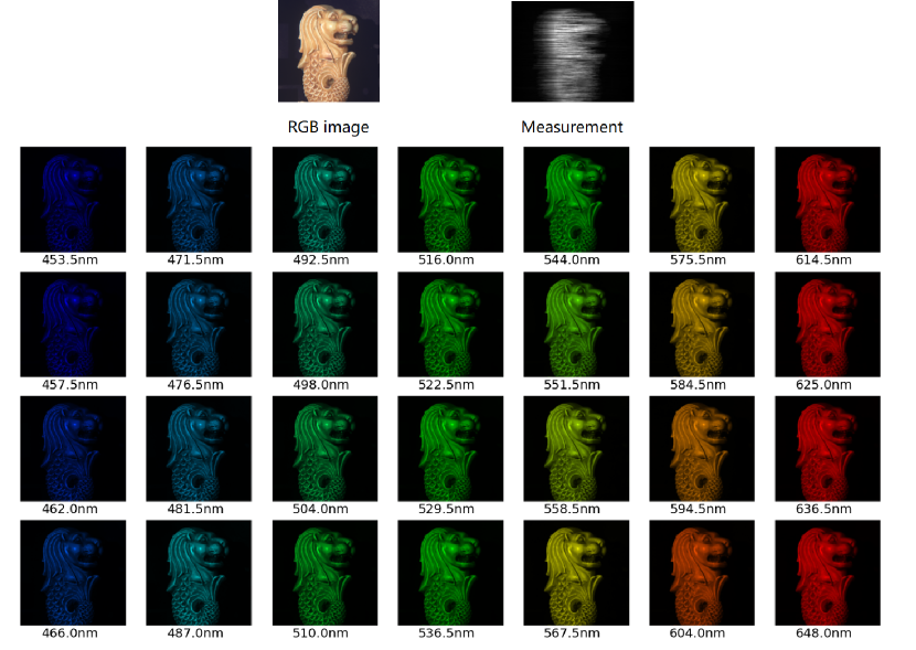
Figure 7: Reconstructed simulation spectral images with 28 wavelengths by our SAUNet

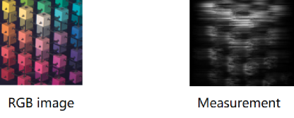
Figure 11: The RGB and Measurement of Scene 2.

To compare the visual results of our network with different unfolding stage numbers, we select Scene 2 of 28 spectral channels to display. Figure 11 shows the RGB image and corresponding to the measurement. Figure 12, 13, 14, 15, 16 and 17 are the reconstructed simulation images of Scene 2 with 28 spectral channels by SAUNet-1stg, SAUNet-2stg, SAUNet-3stg, SAUNet-5stg, SAUNet-9stg and SAUNet-13stg respectively. As we can see, the reconstruction of SAUNet-1stg has been able to achieve a satisfactory result. And with the number of unfolding stages increasing, our reconstruction results recover more fine-grained details and structural textures (Please zoom in for a better view).

Real HSI Reconstruction

Figure 8 depicts the reconstructed real images of Scene 3 with 28 spectral channels. SAUNet-13stg reliably reconstructs all the spectral channels of the desired HSI signal.

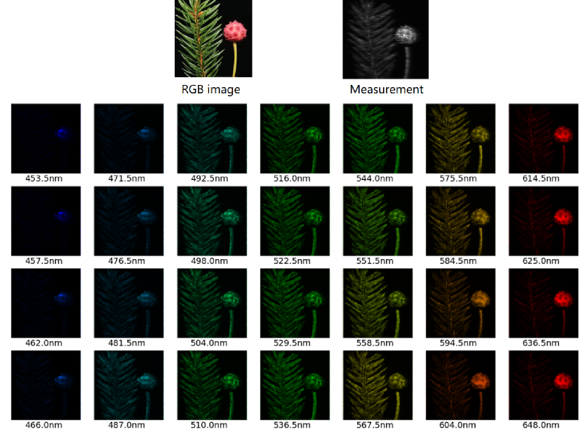
Figure 8: Reconstructed real spectral images with 28 wavelengths by our SAUNet

Appendix E Hyperparameters

Random Seed.

For all experiments of SAUNet, we keep the random seed to 42 in order to reduce the training variances resulting from randomness.

Drop-path Rate.

We use drop-path regularization during training SAUNet. Tabel 6 is our setting for the drop-path rate in each CAB and FFN of encoder blocks and decoder blocks (cdpr) and bottleneck blocks (bdpr). The more stage number of the model is trained, the bigger rate of drop-path we tend to use,

stages	cdpr	bdpr
1	0.0	0.0
2	0.1	0.1
3	0.1	0.2
5	0.1	0.2
9	0.0	0.3
13	0.1	0.2

Table 6: The relationship between the unfolding stage number and rate of drop-path hyperparameter.

Appendix F More ablation studies

Number of Stages for SAUNet.

Figure 9 depicts the curve between PSNR and the number of unfolding stages. Table 5 show the detailed value of PSNR and SSIM among the network with different unfolding stage number. It shows that the performance increases with the number of stages, demonstrating the effectiveness of the iterative network design. And we notice that a 2-stage and 3-stage SAUNet can achieve very impressive PSNR results of 36.73 dB and 37.54dB respectively. With more stages, e.g. non-trivial 13 stages, SAUNet gets continuous PSNR and SSIM improvement.

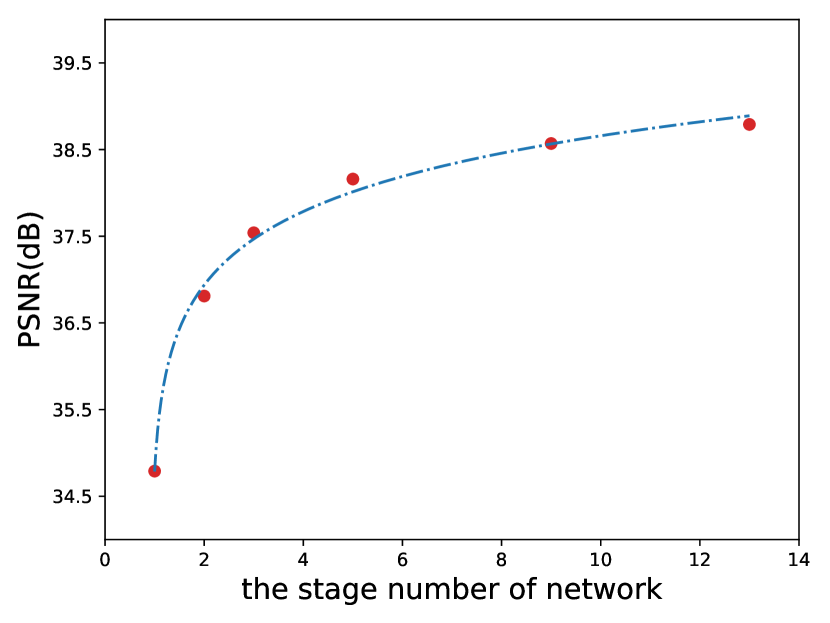
Figure 9: The PSNR-stage curve of our methods.

Number of Stages for Network Components

Tabel 7 shows the influence of different stage numbers on the deep unfolding framework with different denoisers. It demonstrates our R2ADMM framework is still in the lead with different stages and corresponding to different denoisers, compared with HQS and ADMM. It further indicates that the method of relaxing ADMM residuals by setting a series of learnable parameters is robust.

denoiser	stage num	algorithms	PSNR	SSIM
CMFormer	3	w/o	35.77	0.957
CMFormer	3	HQS	37.40	0.966
CMFormer	3	ADMM	37.43	0.965
CMFormer	3	ours	37.54	0.966
CMFormer	5	w/o	36.24	0.962
CMFormer	5	HQS	38.06	0.969
CMFormer	5	ADMM	37.70	0.969
CMFormer	5	ours	38.16	0.970
w/o CAB	3	w/o	23.13	0.559
w/o CAB	3	HQS	29.77	0.736
w/o CAB	3	ADMM	30.13	0.747
w/o CAB	3	ours	30.21	0.751
w/o CAB	5	w/o	23.42	0.571
w/o CAB	5	HQS	30.98	0.773
w/o CAB	5	ADMM	31.04	0.775
w/o CAB	5	ours	31.13	0.778

Table 7: The influence of different stage numbers on the deep unfolding framework with different denoisers.

Self-Attention Mechanism.

To compare convolutional modulation with other self-attention mechanisms (MSA), we adopt a network that is obtained by removing CMB from SAUNet-1stg to conduct the ablation in Tabel 8. For fairness, we keep the Params of MSAs the same by fixing the number of channels and heads. Without any MSA, the network can yield 32.79 dB PSNR. After we implement global (G-MSA) Dosovitskiy et al. (2020), Swin MSA (SW-MSA) Liu et al. (2021), Spectral-wise MSA (S-MSA) Cai et al. (2022a), and HS-MSA Cai et al. (2022c). Following the ablation study of DAUHST, we downsample the input feature maps of G-MSA to avoid memory bottlenecks. We discover that our CMB can gain 2.05 dB, which is 1.21, 1.09, 1.02 dB and 0.79 dB higher than H-MSA, SW-MSA, S-MSA and HS-MSA respectively. This shows that large convolution kernel modulation is good at extracting local and non-local information jointly.

Method	PSNR	SSIM	params (M)	GFLOPs
w/o	32.79	0.904	0.40	6.85
G-MSA	33.63	0.920	0.48	10.30
SW-MSA	33.75	0.924	0.48	9.41
S-MSA	33.82	0.926	0.48	8.89
HS-MSA	34.05	0.930	0.48	9.72
CMB	34.84	0.946	0.78	9.52

Table 8: Ablation of various self-attention mechanisms

Parameters of Unfolding Framework.

To study the effect of the estimated parameters, we perform the break-down ablation of SAUNet. We apply SAUNet-3stg without any estimated parameters as baseline and results are shown in Table 9. It has verified that learnable parameters $\gamma$ are beneficial for the connection between each network component.

For further exploration of the roles’ the estimated parameters, we plot the curves of $\alpha$,$\beta$,$\gamma$ as they change with the iteration in Figure 10 and calculate the PSNR and SSIM results of $\boldsymbol{x}_{k}$ and $\boldsymbol{z}_{k}$ in Tabel 10. We observe that network outputs yield either blurry or noisy images at the early stage, and the $\alpha_{1}$ is a large value. With the iteration number increasing, the gap between $\boldsymbol{x}_{k}$ and $\boldsymbol{z}_{k}$ decreases substantially and the $\alpha$ becomes a small value. For $\gamma$, the values float around 0. it may regulate the connection between each stage and make the network produce a stable output.

baseline	$\alpha$	$\beta$	$\gamma$	PSNR	SSIM
✓	✓			37.14	0.963
✓		✓		37.17	0.964
✓	✓	✓		37.43	0.965
✓	✓	✓	✓	37.54	0.966

Table 9: Ablation of unfolding framework parameters

Metric	$z_{0}$	$x_{1}$	$z_{1}$	$x_{2}$	$z_{12}$	$z_{13}$
PSNR	17.65	19.91	25.24	20.02	38.47	38.79
SSIM	0.265	0.489	0.713	0.497	0.966	0.974

Table 10: Each stage output of unfolding framework parameters

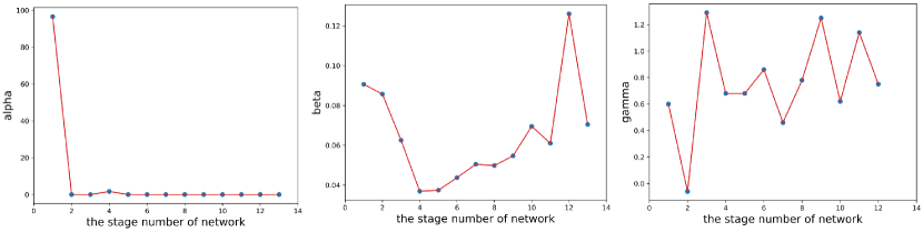
Figure 10: The params-stage curve of SAUNet-13stg.

More Unfolding Framework.

We compare our R2ADMM with previous unfolding frameworks including DAUF Cai et al. (2022c), ADMM-Net Ma et al. (2019), GAP-Net Meng et al. (2020a). For a fair comparison, we replace each single-stage network of DAUHST, ADMM-Net, and GAP-Net with CMFormer. We apply the experiments in 3-stage and the results are shown in Table 11. Our R2ADMM outperforms DAUF, ADMM-Net, and GAP-Net by 0.14 dB, 1.62 dB, and 3.11 dB respectively. While adding only 0.05M parameters and 6.30 GFLOPS compared to ADMM-Net and GAP-Net. This is mainly because the parameters in SAUNet can capture the information on CASSI degradation patterns to provide the cues for HSI reconstruction.

Framework	PSNR	SSIM	params (M)	GFLOPs
GAP	34.43	0.938	2.18	20.01
ADMM	35.92	0.951	2.18	20.01
DAUF	37.40	0.966	2.23	26.31
R2ADMM	37.54	0.966	2.23	26.31

Table 11: Ablation of different unfolding frameworks

Appendix G Limitations

The major limitation of our work is that the performance improvement of our method comes with lowering the inference speed, increasing the model complexity and spending more time training. For example, we can learn that SAUNet-13stg achieves 3.95dB improvement compared with SAUNet-1stg, but it requires $11.6\times$ FLOPs, $10.9\times$ Params, $10.3\times$ inference times, and $5.03\times$ training GPU hours in a Tesla v100 GPU. Although it is a common limitation of this kind of algorithm, we will further study how to improve the restoration results without substantially increasing the model complexity and sacrificing the inference speed and training time for better practical use.

Appendix H Broader impacts

HSIs with rich multi-spectrum and 2D spatial information can better describe the nature of scenes than traditional RGB images, which makes it a widespread application, such as agriculture Lu et al. (2020), medicine Kado et al. (2018), remote sensing Bioucas-Dias et al. (2013) and object detection Kim et al. (2012); Xu et al. (2015). Among the plentiful methods to acquire hyperspectral images, the researchers pay more attention to the coded aperture snapshot compressive imaging (CASSI) systems Wagadarikar et al. (2008) with efficient memory/bandwidth Meng et al. (2020a), low power, and high speed to capture the 3D signal through 2D sensors. The core of CASSI is to develop a coded aperture mask to modulate the HSI signal and compress it into a 2D measurement. Therefore, the worthy research problem is to design a reliable and fast reconstruction algorithm to recover target signals from a 2D compressed image.

Until now, HSI reconstruction techniques had no negative social impact yet. Our proposed SAUNet does not present any negative foreseeable societal consequence, either.

Figure 12: Reconstructed simulation spectral images in Scene 2 with 28 wavelengths by our SAUNet-1stg

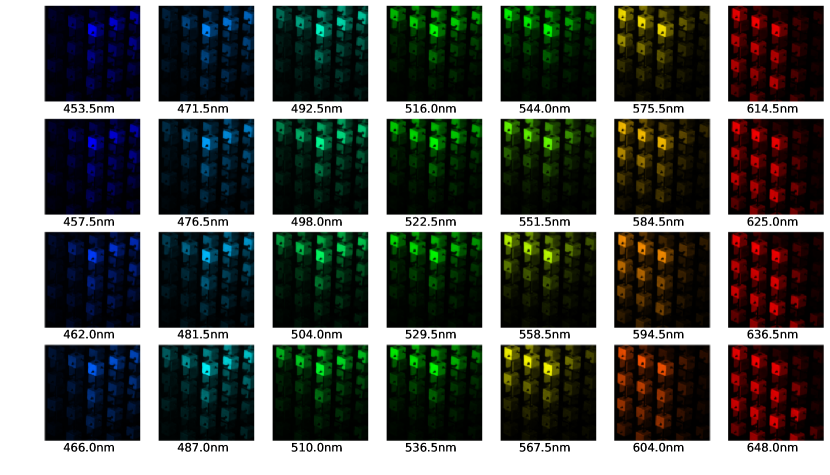
Figure 13: Reconstructed simulation spectral images in Scene 2 with 28 wavelengths by our SAUNet-2stg

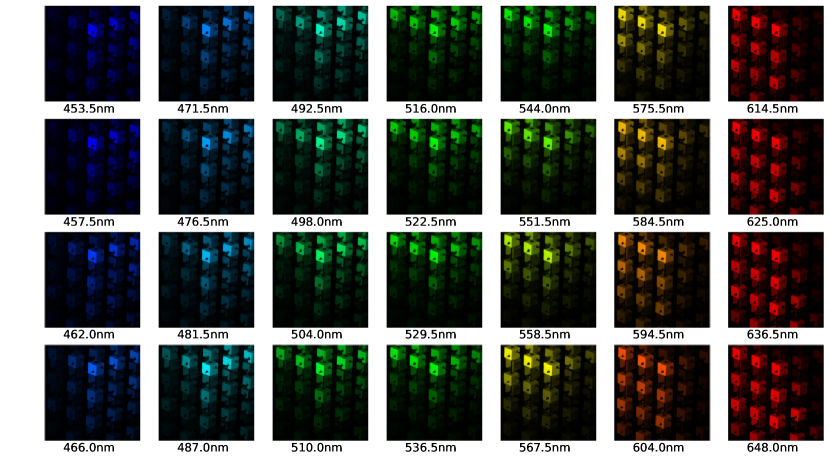
Figure 14: Reconstructed simulation spectral images in Scene 2 with 28 wavelengths by our SAUNet-3stg

Figure 15: Reconstructed simulation spectral images in Scene 2 with 28 wavelengths by our SAUNet-5stg

Figure 16: Reconstructed simulation spectral images in Scene 2 with 28 wavelengths by our SAUNet-9stg

Figure 17: Reconstructed simulation spectral images in Scene 2 with 28 wavelengths by our SAUNet-13stg

References

- Beck and Teboulle [2009] Amir Beck and Marc Teboulle. A fast iterative shrinkage-thresholding algorithm for linear inverse problems. In SIIMS, 2009.
- Bioucas-Dias and Figueiredo [2007] José M Bioucas-Dias and Mário A. T. Figueiredo. A new twist: Two-step iterative shrinkage/thresholding algorithms for image restoration. In TIP, 2007.
- Bioucas-Dias et al. [2013] José M Bioucas-Dias, Antonio Plaza, Gustavo Camps-Valls, Paul Scheunders, Nasser Nasrabadi, and Jocelyn Chanussot. Hyperspectral remote sensing data analysis and future challenges. In TGRS, 2013.
- Boyd et al. [2011] Stephen Boyd, Neal Parikh, Eric Chu, Borja Peleato, Jonathan Eckstein, et al. Distributed optimization and statistical learning via the alternating direction method of multipliers. In Found. Trends Mach. Learn., 2011.
- Cai et al. [2022a] Yuanhao Cai, Jing Lin, Xiaowan Hu, Haoqian Wang, Xin Yuan, Yulun Zhang, Radu Timofte, and Luc Van Gool. Mask-guided spectral-wise transformer for efficient hyperspectral image reconstruction. In CVPR, 2022.
- Cai et al. [2022b] Yuanhao Cai, Jing Lin, Xiaowan Hu, Haoqian Wang, Xin Yuan, Yulun Zhang, Radu Timofte, and Luc Van Gool. Coarse-to-fine sparse transformer for hyperspectral image reconstruction. In ECCV, 2022.
- Cai et al. [2022c] Yuanhao Cai, Jing Lin, Haoqian Wang, Xin Yuan, Henghui Ding, Yulun Zhang, Radu Timofte, and Luc Van Gool. Degradation-aware unfolding half-shuffle transformer for spectral compressive imaging. arXiv:2205.10102, 2022.
- Chen et al. [2016] Tianqi Chen, Bing Xu, Chiyuan Zhang, and Carlos Guestrin. Training deep nets with sublinear memory cost. arXiv:1604.06174, 2016.
- Cheng et al. [2022] Ziheng Cheng, Bo Chen, Ruiying Lu, Zhengjue Wang, Hao Zhang, Ziyi Meng, and Xin Yuan. Recurrent neural networks for snapshot compressive imaging. In TPAMI, 2022.
- Choi et al. [2017] Inchang Choi, Daniel S. Jeon, Giljoo Nam, Diego Gutierrez, and Min H. Kim. High-quality hyperspectral reconstruction using a spectral prior. In SIGGRAPH Asia, 2017.
- Ding et al. [2022] Xiaohan Ding, Xiangyu Zhang, Jungong Han, and Guiguang Ding. Scaling up your kernels to 31x31: Revisiting large kernel design in cnns. In CVPR, 2022.
- Dosovitskiy et al. [2020] Alexey Dosovitskiy, Lucas Beyer, Alexander Kolesnikov, Dirk Weissenborn, Xiaohua Zhai, Thomas Unterthiner, Mostafa Dehghani, Matthias Minderer, Georg Heigold, Sylvain Gelly, et al. An image is worth 16x16 words: Transformers for image recognition at scale. arXiv:2010.11929, 2020.
- He et al. [2013] Ran He, Wei-Shi Zheng, Tieniu Tan, and Zhenan Sun. Half-quadratic-based iterative minimization for robust sparse representation. In TPAMI, 2013.
- Heide et al. [2016] Felix Heide, Steven Diamond, Matthias Nießner, Jonathan Ragan-Kelley, Wolfgang Heidrich, and Gordon Wetzstein. Proximal: Efficient image optimization using proximal algorithms. In TOG, 2016.
- Hou et al. [2022] Qibin Hou, Cheng-Ze Lu, Ming-Ming Cheng, and Jiashi Feng. Conv2former: A simple transformer-style convnet for visual recognition. arXiv:2211.11943, 2022.
- Hu et al. [2022] Xiaowan Hu, Yuanhao Cai, Jing Lin, Haoqian Wang, Xin Yuan, Yulun Zhang, Radu Timofte, and Luc Van Gool. Hdnet: High-resolution dual-domain learning for spectral compressive imaging. In CVPR, 2022.
- Huang et al. [2021] Tao Huang, Weisheng Dong, Xin Yuan, Jinjian Wu, and Guangming Shi. Deep gaussian scale mixture prior for spectral compressive imaging. In CVPR, 2021.
- Kado et al. [2018] Shiika Kado, Yusuke Monno, Kenta Moriwaki, Kazunori Yoshizaki, Masayuki Tanaka, and Masatoshi Okutomi. Remote heart rate measurement from rgb-nir video based on spatial and spectral face patch selection. In EMBC, 2018.
- Kim et al. [2012] Min H Kim, Todd Alan Harvey, David S Kittle, Holly Rushmeier, Julie Dorsey, Richard O Prum, and David J Brady. 3d imaging spectroscopy for measuring hyperspectral patterns on solid objects. In TOG, 2012.
- Kittle et al. [2010] David Kittle, Kerkil Choi, Ashwin Wagadarikar, and David J Brady. Multiframe image estimation for coded aperture snapshot spectral imagers. In Applied Optics, 2010.
- Liu et al. [2018a] Risheng Liu, Xin Fan, Shichao Cheng, Xiangyu Wang, and Zhongxuan Luo. Proximal alternating direction network: A globally converged deep unrolling framework. In AAAI, 2018.
- Liu et al. [2018b] Yang Liu, Xin Yuan, Jinli Suo, David J Brady, and Qionghai Dai. Rank minimization for snapshot compressive imaging. In TPAMI, 2018.
- Liu et al. [2019] Qinghua Liu, Xinyue Shen, and Yuantao Gu. Linearized admm for nonconvex nonsmooth optimization with convergence analysis. In IEEE Access, 2019.
- Liu et al. [2021] Ze Liu, Yutong Lin, Yue Cao, Han Hu, Yixuan Wei, Zheng Zhang, Stephen Lin, and Baining Guo. Swin transformer: Hierarchical vision transformer using shifted windows. In ICCV, 2021.
- Liu et al. [2022] Zhuang Liu, Hanzi Mao, Chao-Yuan Wu, Christoph Feichtenhofer, Trevor Darrell, and Saining Xie. A convnet for the 2020s. In CVPR, 2022.
- Lu et al. [2020] Bing Lu, Phuong D Dao, Jiangui Liu, Yuhong He, and Jiali Shang. Recent advances of hyperspectral imaging technology and applications in agriculture. In Remote Sensing, 2020.
- Ma et al. [2019] Jiawei Ma, Xiao-Yang Liu, Zheng Shou, and Xin Yuan. Deep tensor admm-net for snapshot compressive imaging. In ICCV, 2019.
- Meng et al. [2020a] Ziyi Meng, Shirin Jalali, and Xin Yuan. Gap-net for snapshot compressive imaging. arXiv:2012.08364, 2020.
- Meng et al. [2020b] Ziyi Meng, Jiawei Ma, and Xin Yuan. End-to-end low cost compressive spectral imaging with spatial-spectral self-attention. In ECCV, 2020.
- Meng et al. [2020c] Ziyi Meng, Mu Qiao, Jiawei Ma, Zhenming Yu, Kun Xu, and Xin Yuan. Snapshot multispectral endomicroscopy. In Optics Letters, 2020.
- Miao et al. [2019] Xin Miao, Xin Yuan, Yunchen Pu, and Vassilis Athitsos. lambda-net: Reconstruct hyperspectral images from a snapshot measurement. In ICCV, 2019.
- Mittal et al. [2012] Anish Mittal, Rajiv Soundararajan, and Alan C Bovik. Making a “completely blind” image quality analyzer. In SPL, 2012.
- Monga et al. [2021] Vishal Monga, Yuelong Li, and Yonina C. Eldar. Algorithm unrolling: Interpretable, efficient deep learning for signal and image processing. In SPM, 2021.
- Park and Kim [2022] Namuk Park and Songkuk Kim. How do vision transformers work? arXiv:2202.06709, 2022.
- Qiao et al. [2020] Mu Qiao, Ziyi Meng, Jiawei Ma, and Xin Yuan. Deep learning for video compressive sensing. In APL Photonics, 2020.
- Ronneberger et al. [2015] Olaf Ronneberger, Philipp Fischer, and Thomas Brox. U-net: Convolutional networks for biomedical image segmentation. In MICCAI, 2015.
- Ross et al. [2021] Wightman Ross, Touvron Hugo, and Jégou Hervé. Resnet strikes back: An improved training procedure in timm. arxiv:2110.00476, 2021.
- Wagadarikar et al. [2008] Ashwin Wagadarikar, Renu John, Rebecca Willett, and David Brady. Single disperser design for coded aperture snapshot spectral imaging. In Applied Optics, 2008.
- Wang et al. [2020] Lizhi Wang, Chen Sun, Maoqing Zhang, Ying Fu, and Hua Huang. Dnu: Deep non-local unrolling for computational spectral imaging. In CVPR, 2020.
- Xu et al. [2015] Yang Xu, Zebin Wu, Jun Li, Antonio Plaza, and Zhihui Wei. Anomaly detection in hyperspectral images based on low-rank and sparse representation. In TGRS, 2015.
- Xu et al. [2016] Zheng Xu, Mário A. T. Figueiredo, and Thomas A. Goldstein. Adaptive admm with spectral penalty parameter selection. In AISTATS, 2016.
- Xu et al. [2017] Zheng Xu, Mário A. T. Figueiredo, Xiaoming Yuan, Christoph Studer, and Tom Goldstein. Adaptive relaxed admm: Convergence theory and practical implementation. In CVPR, 2017.
- Yang et al. [2022] Jianwei Yang, Chunyuan Li, and Jianfeng Gao. Focal modulation networks. arXiv:2203.11926, 2022.
- Yasuma et al. [2010] Fumihito Yasuma, Tomoo Mitsunaga, Daisuke Iso, and Shree K Nayar. Generalized assorted pixel camera: postcapture control of resolution, dynamic range, and spectrum. In TIP, 2010.
- Yuan [2016] Xin Yuan. Generalized alternating projection based total variation minimization for compressive sensing. In ICIP, 2016.