Neuronal architecture extracts statistical temporal patterns

Abstract

Neuronal systems need to process temporal signals. We here show how higher-order temporal (co-)fluctuations can be employed to represent and process information. Concretely, we demonstrate that a simple biologically inspired feedforward neuronal model is able to extract information from up to the third order cumulant to perform time series classification. This model relies on a weighted linear summation of synaptic inputs followed by a nonlinear gain function. Training both – the synaptic weights and the nonlinear gain function – exposes how the non-linearity allows for the transfer of higher order correlations to the mean, which in turn enables the synergistic use of information encoded in multiple cumulants to maximize the classification accuracy. The approach is demonstrated both on a synthetic and on real world datasets of multivariate time series. Moreover, we show that the biologically inspired architecture makes better use of the number of trainable parameters as compared to a classical machine-learning scheme. Our findings emphasize the benefit of biological neuronal architectures, paired with dedicated learning algorithms, for the processing of information embedded in higher-order statistical cumulants of temporal (co-)fluctuations.

I Introduction

It has long since been hypothesized that information about the environment and internal states of humans and animals is represented in the correlated neuronal activity. The most apparent examples include spike patterns that are related to organization of cognitive motor processes and visual perception [53, 38, 61, 60]. Such patterns are also quantified indirectly via neuronal rhythms [56, 46, 58, 18]. Furthermore, the variability of network responses across trials when presenting the same stimulus [4] has been firstly shown to limit encoding robustness, but was later found to serve a functional role in a Bayesian context to represent (un)certainty about the presented stimulus [6, 49].

Structured variability is likely to play an important role in learning by interacting with synaptic plasticity, in particular for models like spike-timing-dependent plasticity (STDP) that are sensitive to high-order statistics [21, 9, 25, 22]. STDP implements an unsupervised learning rule similar to classical Hebbian learning based on firing rates [28, 32] and the BCM learning rule [7, 1, 35]. A counterpart for supervised learning has recently been proposed as a basis for neuronal representations, which reconciles the apparent contradiction between robust encoding by seemingly noisy signals [24]. This can be achieved by detecting and selecting correlated patterns thanks to an adequate learning rule to update the synaptic weights between neurons, thereby implementing a form of “statistical processing”. The focus on second-order statistics as a measure for spike trains complements recent supervised learning schemes which either shape the detailed spiking time generated by neurons or control their time-varying firing rates [27, 50, 71].

An adjoint viewpoint to this biologically inspired learning is taken up by machine learning. Though constructed from similar building blocks (so called artificial neurons), the focus here lies in finding optimal and efficient (re)encoding to process large amounts of data, the most widespread application being classification. This field has produced artificial neuronal architectures with impressive performance, even better than human performance in the case of image recognition (see [41, 2] for reviews). However, time series, which are naturally processed by biological neuronal systems, can be challenging for these systems. For example, they are often designed to operate on a feature space with fixed dimensionality (including duration) as opposed to the learning of ongoing signals that may have variable lengths. In this setting, artificial neural networks are designed to account for different input durations across samples. Recurrent neural networks, with their time-dependent network states, handle these inputs by construction. Reservoir computing [36, 42], which has been recently employed to capture statistical differences in the input cumulants [47], forms a straightforward implementation of a trainable recurrent neural network. Also long-short term memory (LSTM) units [33] or the more recent Gated Recurrent Units [11] employ feedback connections to process time series.

Time series processing has increasingly raised interest at the intersection of biological learning and machine learning, based on a diversity of network architectures and approaches [5, 57]. Many studies rely on feedforward networks that have proven to be efficient [67, 19]; recurrent networks, in contrast, are notoriously harder to train [72, 34], despite progress for specific applications like time series completion [65, 13]. Reservoir computing consists in an intermediate approach, where a large (usually untrained) recurrent network is combined with an easily trainable feedforward readout. Its processing capabilities come from the combination of recurrent connectivity with nonlinear units that performs complex operations on the input signals, to be then selected by the readout to form the desired output. The training of such feedforward readouts to capture structured variability in a time series is our motivation and focus, leaving out the reservoir here.

The present study considers statistical processing for the classification of temporal signals by a feed-forward neuronal system, aiming to capture structured variability embedded in time series. The goal is to automatically select the relevant statistical orders, possibly combining them to shape the output signal. We focus in this study on classification that relies on the temporal mean of the output, which implies that input cumulants at various orders need to be mapped to the first order in output. The main inspiration is to design a biological setup consisting of neurons that linearly sum input signals weighted by their afferent connectivity weights, before passing the resulting signal to a non-linear gain function. We also compare this biologically inspired architecture with a machine learning approach, in terms of classification accuracy and trainable weights (resources). Fig. 1 displays a concise summary of the setup.

The remainder of this work is structured as follows: We first present the models of neuronal classifiers with two flavors (Section II.1): a biological architecture and a machine learning architecture. We show how they differ by the number of trainable weights (akin to resources) and in their optimization. Then we describe the input time series used to validate and compare these classifiers (Section II.2). We rely on both synthetic data with controlled structures and contrast between the classes as well as on real-world signals coming from Chen et al. 10. Our results start with the synthetic datasets (Section III.1), to test whether the classifiers can extract statistics embedded in time series that are relevant for the classification. In particular, we examine whether the combination of different orders leads to synergistic behavior, namely whether it increases the classification accuracy (Section III.2). Finally, we verify the practical applicability of our framework to real-world datasets, comparing the performances of both architectures to the state of the art (Section III.3).

II Methods

II.1 Neuronal classifiers

FIG. 1: Biological interpretation of an order-selective perceptron. The input time series $x^{t}$ is linearly combined by the connectivity matrix $B$ to form the intermediate variable $y^{t}=Bx^{t}$. The latter is then passed on through a non-linear gain function $\phi$ to obtain the output $z^{t}$. The classification decision is made with respect to the temporal average of $z^{t}$, which has the dimensionality of the number of classes to predict, in a winner-take-all fashion. The gain function $\phi$ is implemented by a third-order polynomial with coefficients $\alpha_{1}$, $\alpha_{2}$, $\alpha_{3}$. The contributions for orders two and three are the Taylor coefficients of $\phi$ evaluated at the temporal mean of $\langle y^{t}\rangle_{t}$ over the duration of the input. In contrast, the linear contribution directly acts on $z^{t}$. In the present figure, we consider $5$ input signals and $3$ output neurons, one of which is shown upfront.

We consider classification of multi-variate time series by a biologically inspired neuronal architecture illustrated in Fig. 1 that we term “order selective perceptron” (OSP). The multivariate input time series $x_{i}^{t}$ with $1\leq i\leq N$ is linearly combined via the trainable connectivity matrix $B_{ji}\in\mathbb{R}^{M\times N}$ to form the intermediate time-dependent variable $y_{j}^{t}=\sum_{i}B_{ji}x_{i}^{t}$. Here $1\leq j\leq M$, where $M$ is the number of classes to be distinguished. Then, a non-linear gain function $\phi$ is applied on $y_{j}^{t}$, taken as a univariate signal, to obtain the output $z_{j}^{t}=\phi(y_{j}^{t})$. Classification is performed based on the temporal mean (first-order statistics) $Z_{j}=\langle z_{j}^{t}\rangle$. This gain function $\phi$ is shaped to combine the cumulants of the intermediate variable $y_{j}^{t}$, where the $n$-th statistical cumulant (evaluated over time) of $y_{j}^{t}$ is denoted as $\langle\!\langle\big{(}y_{j}^{t}\big{)}^{n}\rangle\!\rangle_{t}=Y_{j}^{n}$ , resulting in $Z_{j}=\sum_{n}\alpha_{n}\langle\!\langle\big{(}y_{j}^{t}\big{)}^{n}\rangle\!\rangle_{t}=\sum_{n}\alpha_{n}Y_{j}^{n}$. The $n$-th cumulant $Y_{j}^{n}$ reflects the corresponding cumulants at the same order for the multivariate inputs $x_{i}^{t}$ as

$$Y_{j}^{n}=\langle\!\langle\big{(}y_{j}^{t}\big{)}^{n}\rangle\!\rangle_{t}=\sum_{i_{1},\ldots,i_{n}=1}^{N}B_{ji_{1}}\cdots B_{ji_{n}}\langle\!\langle x_{i_{1}}^{t}\cdots x_{i_{n}}^{t}\rangle\!\rangle_{t}\,.$$ (1)

Thus, a general gain function combines several statistical orders of the input to generate the mean $Z_{j}$ of the output activity. Here, we aim to perform the classification based on the first three cumulants. The gain function is therefore implemented as a trainable third-order polynomial of the intermediate variable $y_{j}^{t}$, see the inset panel in Fig. 1.

II.1.1 Link to covariance perceptron

Before explaining the OSP in more detail, we briefly present its operational link with the covariance perceptron [24, 12]. The goal of the latter is to operate on the second-order statistics embedded in the time series, instead of the first-order statistics that is equivalent to the classical perceptron applied to mean activity [54, 44, 68]. It can be formalized as in Fig. 2 (a), where the linear mixing is based on the weight matrix $B_{ji}^{\text{P}}$ applied to the $N$-dimensional time-dependent inputs $x_{i}^{t}$ (after demeaning) gives the $M$-dimensional intermediate variable $y_{j}^{t}$

$$y_{j}^{t}=\sum_{i}B_{ji}^{\text{P}}\left(x_{i}^{t}-\langle x_{i}^{t}\rangle_{t}\right)\,.$$ (2)

From the outer product of $y_{j}^{t}$ that forms the covariance matrix, the classification only considers the variances (diagonal matrix elements) defined as

$$Z_{j} =\langle\!\langle(y_{j}^{t})^{2}\rangle\!\rangle_{t}$$ (3)

$$=[\text{diag}(B^{\text{P}}\Sigma B^{\text{P}\,\mathrm{T}})]_{j}\,.$$ (4)

Thanks to the quadratic operation, the mean value of $Z_{j}$ depends on the input covariances $\Sigma_{ii^{\prime}}=\langle\!\langle x_{i}^{t}x_{i^{\prime}}^{t}\rangle\!\rangle_{t}$ for all possible indices $i$ and $i^{\prime}$. In this scheme, there are only $M\cdot N$ weights in matrix $B^{\text{P}}$ that can be trained. Thus the number of parameters can be compared to a machine-learning approach that applies a perceptron the entries of the covariance matrix $Z_{j}^{\prime}=\sum_{ii^{\prime}}B_{jii^{\prime}}^{\text{ML}}\Sigma_{ii^{\prime}}$, which involves $M\cdot N^{2}$ trainable parameters of the tensor $B^{\text{ML}}$.

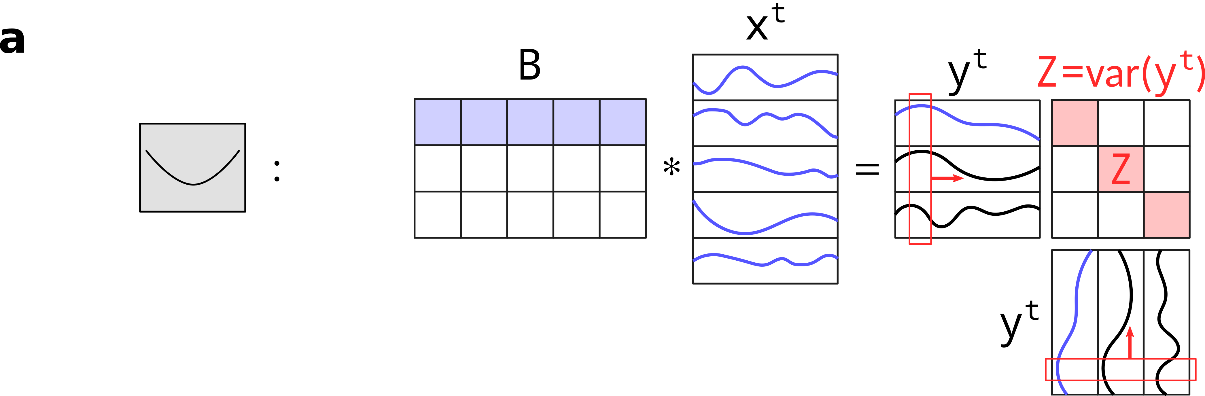
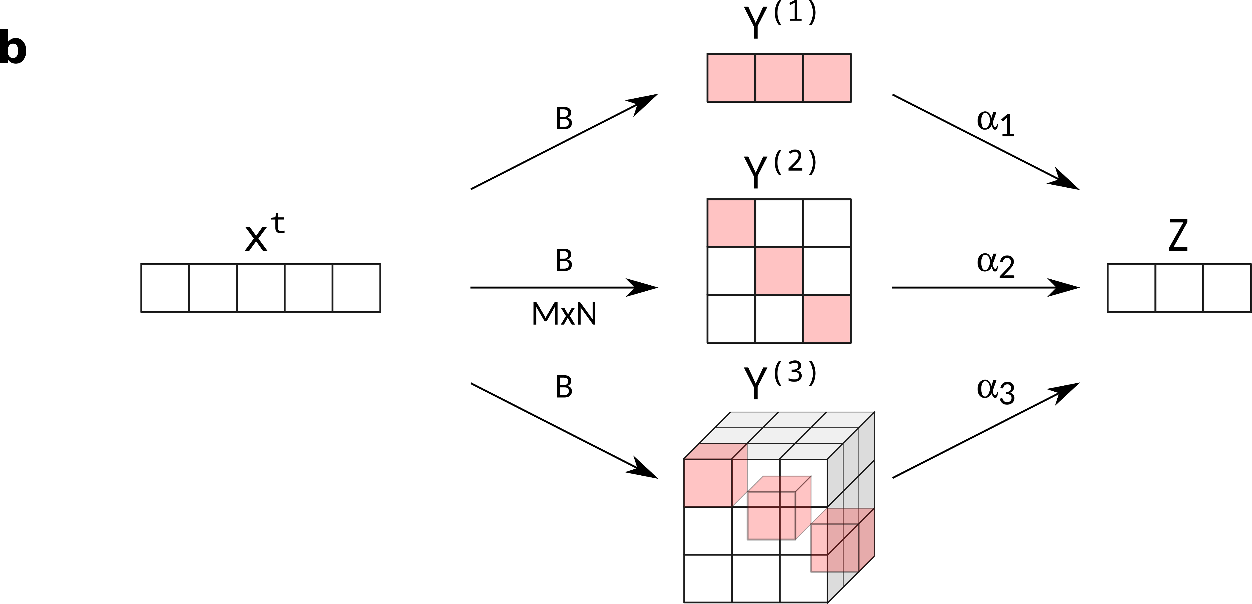
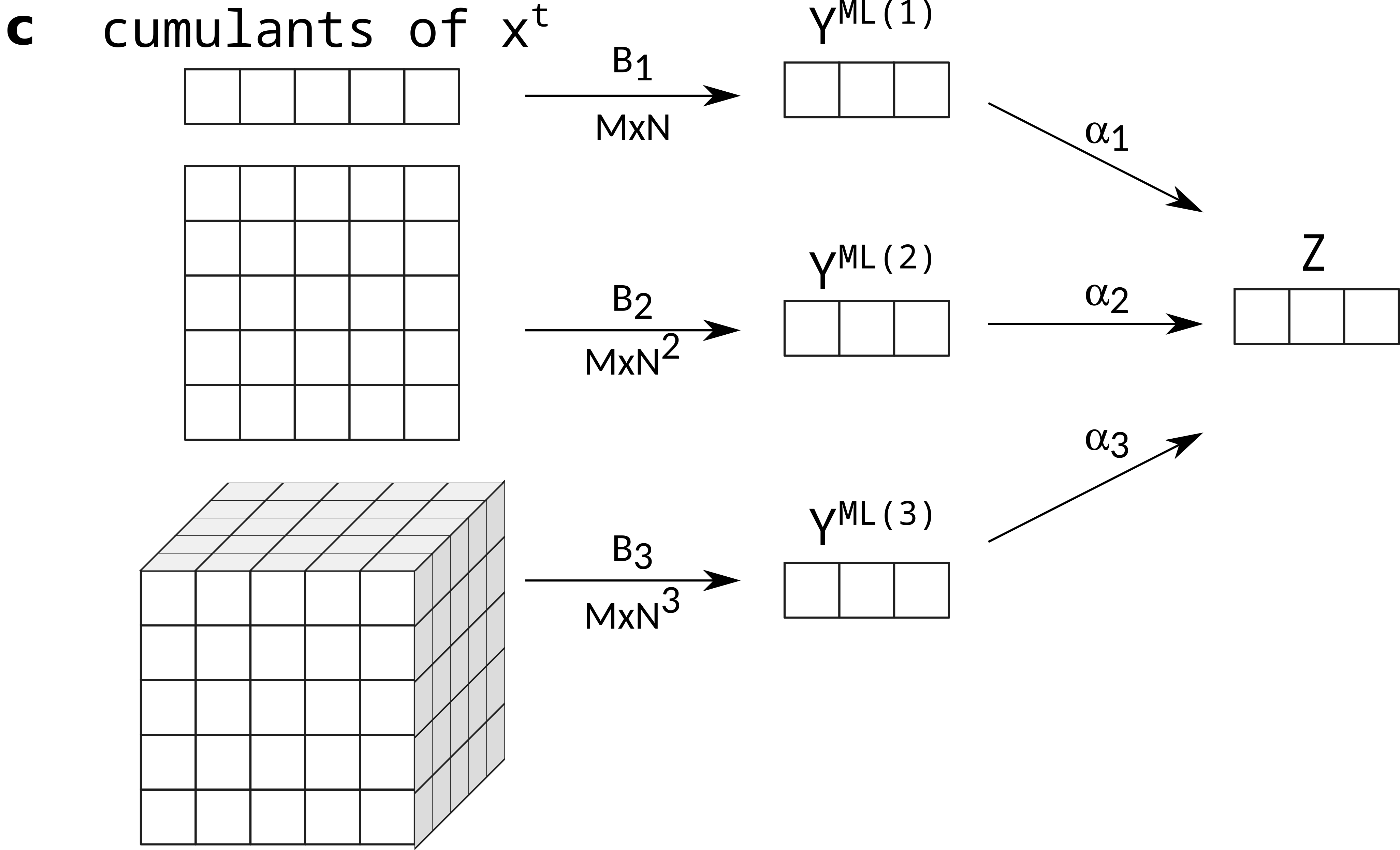
FIG. 2: Extraction of cumulants from a time series. (a) Covariance perceptron. The classification of the centered time series $x^{t}$ is based on its covariance structure. The output $Z=(Z_{1},\ldots,Z_{M})$ has dimension equal to the number of classes $M$. For each class $j$ ($1\leq j\leq M)$, the covariance perceptron calculates an intermediate variable $y_{j}^{t}=\sum_{i}B_{ji}x_{i}^{t}$ that is then passed though a quadratic function $z_{j}^{t}=(y_{j}^{t})^{2}$. The temporal mean $Z_{j}=\langle z_{j}^{t}\rangle=\langle\!\langle(y_{j}^{t})^{2}\rangle\!\rangle_{t}$, which therefore equals the variance of $y^{t}$ is used for classification in a winner-take-all manner. This is equivalent to retaining the diagonal of the covariance matrix of $y_{1\leq j\leq M}^{t}$. (b) Statistical processing for order selective perceptron (OSP) model. Similar to panel (a), the effect of the gain function $\phi$ in Fig. 1 can be represented by an individual path for each cumulant $\langle\!\langle\big{(}y_{j}^{t}\big{)}^{n}\rangle\!\rangle_{t}$ of $y_{j}^{t}=\sum_{i}B_{ji}x_{i}^{t}$. The cumulants of $y^{t}$ are thus given by the cumulants of the inputs $x^{t}$ of the same order $n$ (Eq. (1)). The cumulant of order $n$ can be seen as an outer product with dimensionality $M^{n}$:The mean is represented by a line (vector), the covariance by a square (matrix; as in panel a) and the third order cumulant by a cube (third order tensor). The effect of applying the polynomial $\phi(y)=\alpha_{1}y+\alpha_{2}\tilde{y}^{2}+\alpha_{3}\tilde{y}^{3}$ with $\tilde{y}^{t}=y^{t}-\langle y^{t}\rangle_{t}$ and then taking the mean to obtain $Z$ is to combine these contributions linearly with a weight vector $\alpha=(\alpha_{1},\alpha_{2},\alpha_{3})$ . (c) Machine-learning (ML) model. Statistical processing can alternatively be implemented by a network that is fed by the input cumulants directly. For each order, a linear layer is set up with the corresponding dimensionality: the total size of the input cumulant multiplied by the number of outputs (i.e. of classes). In a second layer, a linear combination of the outputs for the individual orders is trained.

II.1.2 Order selective perceptron (OSP)

Now we consider the order selective perceptron (OSP), a feedforward network that extends the covariance perceptron to combine the first three statistical orders of the input time series $x^{t}$ via the calculation of the output time series $z^{t}$, illustrated in Fig. 1, as

$$y_{j}^{t} =\sum_{i}B_{ji}x_{i}^{t}\,,$$ (5)

$$z^{t} =\phi(y^{t})\>=\alpha_{1}y+\alpha_{2}\tilde{y}^{2}+\alpha_{3}\tilde{y}^{3}.$$ (6)

Here the linear weights $B_{ji}$ are trainable, as well as the coefficients $\alpha_{1\leq i\leq 3}$ of the (nonlinear) polynomial gain function $\phi$. Note that $\tilde{y}^{t}=y^{t}-\langle y^{t}\rangle_{t}$ is the demeaned version of time series $y^{t}$.

The key of the statistical processing is the following: the cumulants at orders 1 to 3 can be calculated using the polynomial of order 3 applied to the intermediate variable $y_{j}^{t}$, as the second and third cumulants are the central moments (including the demeaning). An abstract representation of the resulting computation is illustrated in Fig. 2 (b). Each path of the network corresponding to a specific cumulant of order $n$ of the intermediate variable $y^{t}$. The OSP computation can thus be understood via the cumulants of order $n\in\{1,2,3\}$ of $y_{j}^{t}$ as illustrated in Fig. 2(b)

$$Y_{j}^{(\!n\!)} =\langle\!\langle(y_{j}^{t})^{n}\rangle\!\rangle_{t}\,,$$ (7)

where the symbol $\langle\!\langle(y_{j}^{t})^{n}\rangle\!\rangle_{t}$ stands for the mean over time $\langle y_{j}^{t}\rangle_{t}$ for $n=1$, and the $n$-th power of the demeaned variable $\langle(y_{j}^{t}-\langle y_{j}^{t}\rangle_{t})^{n}\rangle_{t}=\langle(\tilde{y}^{t})^{n}\rangle_{t}$ for $n\in\{2,3\}$; they correspond to the red diagonal matrix or tensor elements in Fig. 2(b). Importantly, each cumulant $Y_{j}^{(\!n\!)}$ for order $n$ depends on the $n$-th statistical order of $x$ (see also Eq. (1)).

Note that it is straightforward to generalize this scheme to arbitrary cumulant orders, beyond the first three orders considered here, because a cumulant of any order $n$ can be expressed as a linear combination of moments of orders $1,\ldots,n$; beyond third order, however, they cease to be identical to the $n$-th centered moments [20]. The resulting computation of the OSP is thus the combination in the output mean $Z_{j}=\langle z_{j}^{t}\rangle_{t}$ of the different cumulant orders $n$

$$Z_{j}=\sum_{n}\alpha_{n}Y_{j}^{(\!n\!)}\,,$$ (8)

which is the basis for the classification via

$$\arg\max(Z_{j}-\theta_{j})$$ (9)

with some trainable thresholds $\theta_{j}$. The key point here is that the selection of the informative cumulant orders for the classification is managed by tuning the parameters $\alpha_{n}$.

We now want to evaluate how the OSP combines different cumulant orders to perform classification. From the network after training, which we refer to as the “full” model with all coefficients $\alpha_{n}$, we can ignore contributions from given cumulant orders by setting the corresponding parameter $\alpha_{n}$ to zero. In this way, we create a “single order” OSP for order $n$ with $\alpha_{n^{\prime}}=0\quad\forall n{}^{\prime}\neq n$. This network is then classifying based on the $n$-th cumulant only with the corresponding learned parameter $\alpha_{n}$. With this approach we quantify the contribution of an individual statistical order $n$ to classification in the full model.

II.1.3 Machine-learning classifier

For comparison, we consider a machine learning (ML) architecture that computes the same statistical cumulants, as features for a linear perceptron. The operational difference is that the weights directly map all features to the next layer, as displayed in Fig. 2 (c)

$$Y_{j}^{\text{ML}(\!n\!)} =\sum_{i_{1}\ldots i_{n}}B_{ji_{1}\ldots i_{i}}^{\text{ML}(\!n\!)}\langle\!\langle x_{i_{1}}^{t}\cdots x_{i_{n}}^{t}\rangle\!\rangle_{t}^{n}\,,$$ (10)

yielding a number of trainable parameters equal to $MN^{n}$ for order $n$. As before, the different orders are combined and selected using Eq. (8). Note that the ML architecture differs from the OSP in that it outputs scalar values, not a time series. To be able to further compare this ML architecture to the OSP, we randomly select $MN$ trainable weights from the whole $MN^{n}$ entries of $B^{\mathrm{ML}}$ (the other weights being fixed to random values) to build the ’constrained ML’ architecture which has the same number of trainable parameters as the OSP. This way, the complexity of the two systems is comparable.

II.1.4 Training process

Training of both network types is conducted via a stochastic gradient descent using a scaled squared error loss $\varepsilon$ for each data sample $\nu$ of the form

$$\varepsilon(x^{\nu})\sim\frac{1}{2}\sum_{j=1}^{M}\left(\bar{Z}_{j}^{c(\nu)}-(Z_{j}^{\nu}-\theta_{j})\right)^{2}\,,$$ (11)

where $\bar{Z}_{j}^{c(\nu)}=\delta_{j,c(\nu)}$ is the one-hot encoded target for the mean, with $c(\nu)\in\{1,\ldots,M\}$ the ground truth of the class of data sample $\nu$ and $\theta_{j}$ is a trainable bias. In the binary classification problem, the one-hot encoded network output has dimension $M=2$. In addition, we add an L2 regularization term $\mu\,\|\alpha\|^{2}$ to the loss with a fixed, small $\mu$ to decrease the entries of the order selection parameter $\alpha$. This ensures that uninformative layers lead to a vanishing contribution to $\alpha$, but also implements a winner-take-all mechanism when there is a strong imbalance between the difficulty of classification for each individual order. Non-vanishing entries in $\alpha$ hence indicate the contribution of the corresponding statistical order to the classification decision. We therefore quantify the synergy of the OSP by the difference in performance of the full OSP model with models that were pruned after training such that they only use a single order $n$ at a time. This is achieved by setting the parameters $\alpha_{n^{\prime}\neq n}=0$ for the other orders. The participation ratio $\rho$,

$$\rho(\alpha)=\frac{\sum_{n}|\alpha_{n}|}{\left(\sum_{n}|\alpha_{n}|^{2}\right)^{\frac{1}{2}}}\,,$$ (12)

can be used as a measure of sparsity to relate the synergy to how many relevant statistical orders the network found in the data. It is minimal when there is only a single non-zero $\alpha_{n}$ and maximal when all $\alpha_{n}$ are equal. Thus, it increases the more different orders $n$ are combined.

II.2 Synthetic datasets with controlled cumulant structure

We design synthetic datasets to assess the ability of the proposed networks to capture specific statistical orders in the input signals. To that end, we generate two groups of multivariate time series with desired statistics up to the third order. We control how the two groups differ with regard to the first three cumulants. Concretely, the time series are generated by simulating in discrete time a process defined by a stochastic differential equation (SDE), whose samples in the infinite time limit follow a Boltzmann probability distribution

$$p(x)\sim\exp(-\beta L[x]).$$ (13)

Samples $x(t)=\{x_{i}(t)\}$ are produced by the following process defined with $L[x]$ as Lagrangian

$$\frac{\partial x_{i}(t)}{\partial t}=-\Gamma\frac{\partial L[x]}{\partial x_{i}}(t)+\xi_{i}(t)\,.$$ (14)

Here, $\xi$ is the stochastic Gaussian increment (or Wiener process or more colloquially white noise) that obeys $\langle\xi\rangle=0$, $\langle\!\langle\xi_{i}(t),\xi_{j}(t^{\prime})\rangle\!\rangle=D\delta_{ij}\delta(t-t^{\prime})$ and $\Gamma$ is a constant parameter. Using a fluctuation-dissipation theorem [26] one finds that $\beta=2\frac{\Gamma}{D}$ in order for $x$ to follow the distribution (13) shaped by the choice of $L[x]$.

The particular case of a Gaussian distribution corresponds to a quadratic Lagrangian

$$L[x]=m^{T}x+\frac{1}{2}x^{T}Jx\,,$$ (15)

where $J=J^{\mathrm{T}}$ is a symmetric matrix, such that the mean $\mu=\langle x\rangle$ and covariance $\Sigma_{ij}=\langle\!\langle x_{i}x_{j}\rangle\!\rangle$ of the distribution read

$$\mu =-J^{-1}m\,,$$ (16)

$$\Sigma =(\beta J)^{-1}\,,$$ (17)

while the third order, $S_{ijk}=\langle\!\langle x_{i}x_{j}x_{k}\rangle\!\rangle$, vanishes. The more general case with the additional 3rd order statistics can then be developed in the spirit of field theory with a small perturbation (or correction) on the Gaussian case. The corresponding Lagrangian reads

$$L[x]=m^{T}x+\frac{1}{2}x^{T}Jx+\frac{1}{3!}\sum_{ijk}K_{ijk}x_{i}x_{j}x_{k}.$$ (18)

For a sufficiently small tensor $K$, the first three cumulants can be approximated as (See appendix, Section A)

$$\mu_{i} \approx-\sum_{j}(J^{-1})_{ij}m_{j}-\frac{1}{2\beta}\sum_{jkl}(J^{-1})_{ij}K_{jkl}(J^{-1})_{kl}\,,$$ (19)

$$\Sigma_{ij} \approx\frac{1}{\beta}(J^{-1})_{ij}\,,$$ (20)

$$S_{ijk} \approx-\frac{1}{\beta^{2}}\sum_{i^{\prime}j^{\prime}k^{\prime}}K_{i^{\prime}j^{\prime}k^{\prime}}(J^{-1})_{ii^{\prime}}(J^{-1})_{jj^{\prime}}(J^{-1})_{kk^{\prime}}\,.$$ (21)

This approximation only holds for a small deviation from the Gaussian case, which limits the amplitude of the third order statistics. Concretely, we introduce a safety parameter $s$ to ensure that a local minimum of the potential $L[x]$ exists and that the distance between the local minimum and the next maximum is large enough to fit $s$ standard deviations of $x$ in any direction. When integrating the SDE, large $s$ ensures a low probability for a sample initialized in that local minimum to evolve further than the adjacent local maximum and prevents it of falling into the unstable region. In this case, the ratio of third to second order cumulants of $x$, projected to any eigendirection $e^{(\!v\!)}$ of $J$, is maximally allowed to be

$$\left|\frac{\sum_{ijk}S_{ijk}e_{i}^{(\!v\!)}e_{j}^{(\!v\!)}e_{k}^{(\!v\!)}}{\left(\sum_{ij}\Sigma_{ij}e_{i}^{(\!v\!)}e_{j}^{(\!v\!)}\right)^{\frac{3}{2}}}\right|=\frac{1}{s}\,.$$ (22)

In the appendix, Section B, we show how to compute a suitable tensor $K$ under this constraint. Additionally, we redraw samples that deviate too strongly from the local minimum of $L[x]$, which corresponds to introducing an infinite potential wall where $L[x]$ negatively exceeds the local minimum. Due to the low probability mass in that area for sufficient safety $s$, we do not need to account for this potential wall in the cumulant estimates. This way, we avoid issues with the probability density Eq. (13) not being normalizable. Alternatively, it would also be possible to include a positive definite fourth order term in the Lagrangian and account for this in the calculation of the arising data statistics, however the more simple third order with redrawing and a safety parameter $s=5$ proved to work satisfactorily for the purposes of this work.

We create datasets where the classification difficulty is controlled for each statistical order. To do so, we generate time series grouped in two equally-sized classes, whose cumulants differ by a scaling factor that serves as contrast. For example, we draw a reference class with some randomly drawn cumulants. A class contrast of $1.5$ in the mean and $1$ otherwise then corresponds to the second class having $1.5$ times larger mean and all other cumulants exactly the same. Due to the stability constraint, the third order cumulant may not become arbitrarily large. Practically, we use the class with the larger third order as the fixed cumulant and generate the second class from the first using the reciprocal contrast. This way, in any order, the larger cumulant is the contrast times the smaller cumulant.

II.3 Real datasets

We test our model’s ability to classify on a selection of time-series classification datasets that have previously been used as benchmarks [10]. We select a subset of $18$ multivariate time series datasets of which the data dimensionality allows us to compute the cumulants of the classes directly on the input. Before training, we shift and rescale the data to centralize them around zero and obtain unit variance over all data points. This is required because of the unboundedness of the gain function, which is a third order polynomial, as well as numerical stability when computing the cumulants on the data directly.

III Results

We first benchmark the models proposed in Section II.1 with synthetic data generated with controlled statistical patterns (see Section II.2). We show how the trained parameters can be analyzed to infer what statistical orders are relevant for the classification. The trained network parameters $\alpha_{1\leq l\leq 3}$ in particular allow us to determine the optimal gain function for each dataset. Subsequently we study classification of real multivariate time series. We find that the OSP classifies efficiently compared to the ML model and we observe that the various datasets combine the statistical orders in a different way. The optimal network typically operates with a synergy of different orders.

III.1 Benchmarking with synthetic data

Classification may be performed based on one or several statistical orders measured on each sample time series. Each order thus defines a contrast between the two classes, which corresponds to a baseline classification accuracy when using the corresponding statistical order alone to perform the classification. This contrast is controlled by the coefficients of the two classes in the generative model, as explained in Eq. (14) and Eq. (18).

We also compare the respective classification accuracy of the biological and machine learning architectures while varying the class contrasts to see how they are combined. Note that cumulants of orders higher than three are non-vanishing and may also hold information on the classes, but the neuronal networks by construction neglect them. Each of the two classes comprises $100$ samples, which have dimensionality $N=5$ and $T=100$ time steps per sample. We repeat the classification $25$ times. For each binary classification, two of the three contrasts are chosen to be different from $1$, thus contain the information about the class, while the third contrast is the same for both classes, having contrast of unity.

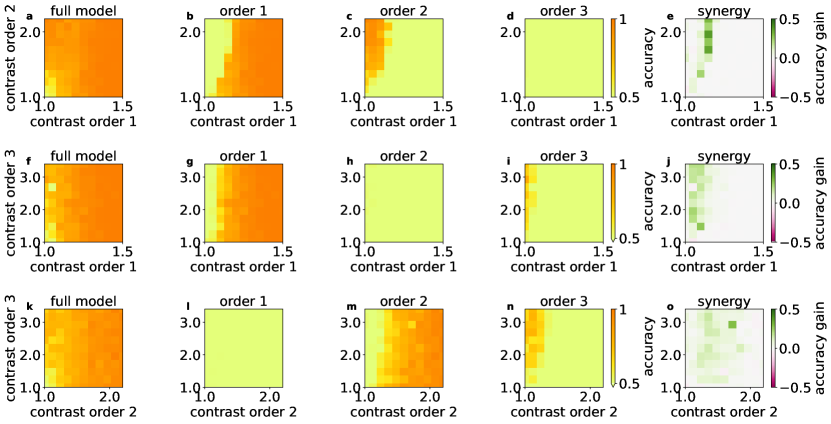
FIG. 3: Classification accuracies for varying task difficulties. Datasets with two equal-sized classes that differ in two statistical orders are classified using the OSP. Along the axes of each diagram the contrast between the two classes is varied between one (no class difference) to an arbitrarily chosen upper scale. (a, f, k) Test set accuracy of the full model. (b, g, l) Accuracy obtained by the OSP when pruning all $\alpha_{n}$ except $\alpha_{1}$ after training. (c, d, h, i, m, n) Analogous to (b) for $\alpha_{2},\alpha_{3}$, respectively. (e, j, o) Synergy, which is the difference in accuracy between the full model and the best single order. In (a - e), classes are separated by a difference in the mean and covariance. In (f - j), classes are separated by a difference in the mean and third order cumulant. In (k - o), classes are separated by a difference in the covariance and third order cumulant.

We start with testing whether the OSP can be efficiently trained to perform classification. Fig. 3 shows the training accuracy for (Gaussian) inputs where the contrasts of orders one and two are varied, while the third cumulant is zero. Accuracy ranges from chance level ($50\%$ for the considered case of two balanced classes, in yellow) to perfect discrimination corresponding to $100\%$ (in orange). Here, successful training means that the OSP captures the most relevant class contrast(s) among the three cumulant orders. As expected, the accuracy of the full model increases when either contrast of order one or two increases (see Fig. 3 (a)).

Investigating the contribution of individual orders in isolation, the accuracy increases with the corresponding contrast between the classes, as shown when varying either order one or two in Fig. 3(b, c). The contribution of the uninformative third order stays chance level Fig. 3(d). In Fig. 3 (f - o), the same qualitative behavior is observed for all different combinations of informative and uninformative orders. This shows that the OSP successfully manages to capture the relevant orders for classification, leading to the question of their combination when two or more orders are relevant.

III.1.1 Synergy between relevant cumulant orders

The accuracy of the full model (Fig. 3 (a)) is larger than the accuracy obtained when single orders are taken individually (Fig. 3 (b-d)). The difference between the accuracy for full training and the maximum of single-order accuracies, shown in Fig. 3 (e), can be used as a measure of synergy: it indicates how the OSP makes use of the combination of the different statistical orders, specifically in the border between the regions of high single-order accuracy. Thus, the OSP (full model) combines the different orders relevant for the classification, beyond simply selecting the most informative order.

We observe a bias between the accuracies for single-order models. Although the synthetic data were generated to have comparable contrasts across the orders, we see that the border where the OSP (full model) switches from one order to another order does not follow a diagonal with equal contrast. This indicates a bias favoring lower statistical orders over higher ones. This may partly come from the fact that higher statistical orders are noisier because they require more time points for estimation. The estimation error causes fluctuations which may affect the training by the parameter updates. In addition to this implicit bias towards extraction of information from lower orders, the normalization imposed on the $\alpha_{n}$ during training (see Section II.1.4 for details) implements a soft winner-take-all mechanism that likely reinforces the bias(es). In Section C, we discuss the accuracy gain of the OSP compared to a restricted OSP, as opposed to the pruned OSP, which can be seen as an alternative way to quantify synergy.

III.1.2 Comparison with machine learning architecture

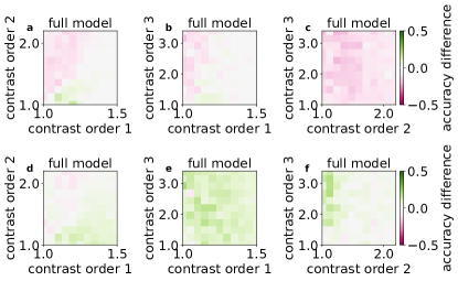
FIG. 4: Comparison of the OSP and the ML model. Difference in accuracy between the OSP and the ML model for the datasets in Fig. 3. (a - c) Accuracy comparison between the ML model and the OSP. (d - f) Accuracy comparison between the constrained ML model and the OSP. The color code shows the difference in accuracy between the respective ML model and the full OSP model.

Last, we compare the OSP to the ML model that has more trainable weights (or resources). As shown in Appendix Section D, the ML network performs well and can discriminate between informative orders. From Fig. 4 (a - c), we find that the accuracy for the OSP is similar to that of the ML, although mostly a bit lower presumably due to its lower number of trainable parameters (weights $B$, compare Fig. 2(b-c)). Nevertheless, it can efficiently combine “information” distributed across statistical orders to perform the classification, and slightly outperform the ML model on mean-based classification.

Presumably this is due to the difference in the number of trainable weights. To test this, we define a ’constrained ML’ network where we subsample $NM$ weights to be trainable, and make sure those are distributed approximately uniformly over the entries of $B^{(\!n\!)}$ for the different orders $n$. The remaining weights stay fixed at their values at initialization. In comparison to the constrained ML model, which has the same number of trainable parameters as the OSP, we typically find a significant performance increase (see Fig. 4 (d - f)).

III.2 Identification of relevant orders from trained parameters

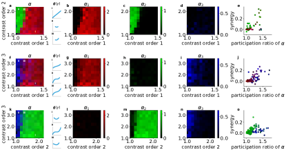
FIG. 5: Readout parameters for varying task difficulties. Datasets with two equal-sized classes which differ in two of their first three cumulants (rows) are classified using the OSP. The weight vector $\alpha=(\alpha_{1},\alpha_{2},\alpha_{3})$ controlling the combination of orders one, two, and three is displayed for the full model (left column) in color code, where the value $\alpha_{n}$ for each order $n$ is displayed by its corresponding rgb value: first order $\alpha_{1}$ (red), second order $\alpha_{2}$ (green), and third order $\alpha_{3}$ (blue). Insets show the corresponding gain function at different points of the parameter regime for the OSP. The second to forth column, respectively, show the individual values of each $\alpha_{1\leq i\leq 3}$. The synergy is displayed over the participation ratio of $\alpha$ (right column). On the axes of each plot the contrast between the classes is varied, starting from one (no class difference) to an arbitrarily chosen upper scale.

In the trained OSP, the $\alpha$ values describe how the different input cumulants are combined in the readout to achieve classification; see Methods for details, Fig. 2(b). All parameters prior to the application of the non-linear gain function are the same for each statistical order. One may therefore interpret the absolute value of each component $|\alpha_{n}|$ as a measure of the contribution of order $n$ to the classification. In Fig. 5 each order $n$ is color-coded in red (mean), green (covariance) and blue (third order), and the color value is proportional to $|\alpha_{n}|$, scaled by the reciprocal of the largest $|\alpha_{n}|$ of all datasets.

As expected, the values $|\alpha_{n}|$ increase depending on the input contrasts corresponding to cumulant order $n$. Again, we find suppression in $\alpha$ due to the competition between the orders when the contrast in one of the informative orders dominates over the other. In contrast to the single order accuracy, however, we here find overlapping regions of non-vanishing $\alpha_{n}$ corresponding to the individual informative orders $n$. These are necessary to form the synergy regions found in Fig. 3. Thus, both informative orders are detected in this region. We find again in Fig. 5 the effect of the bias in Section III.1 that favors lower cumulant orders over higher ones in the training, which is further amplified by the normalization imposed on the $\|\alpha\|$.

In Fig. 3, we observed a synergy effect in the performance along the boundary between regions where individual cumulant orders dominate the classification. These regions coincide with the regions where only one individual $\alpha_{n}$ is non-vanishing. On the boundary between two such regions, both the corresponding $\alpha$ are non-vanishing. To confirm that the synergy is indeed linked to this boundary, we display the synergy found in Fig. 3 to the participation ratio of $\alpha$ (Eq. (12)), which we use as a measure of sparsity here. Indeed, the measures are correlated, although the participation ratio does not account for the fact that $\alpha_{n}$ scales up to different maxima for each order $n$.

We next investigate the corresponding nonlinear gain function $\phi$ shaped by the trained $\alpha$. Noticeably, higher order components contribute significantly despite their lower combination parameter $\alpha_{n}$. We display the gain functions after training for three contrast combinations per synthetic dataset, see insets (i), (ii) and (iii) in Fig. 5. The regions are dominated by a single order, so the gain functions are nearly ideal linear, quadratic, or cubic functions, as expected. In the synergy regions, more complex gain functions arise.

We would like to highlight that the identification of the optimal gain function is specific to the network architecture of the OSP. Although in the ML network, efforts can be made to make $\alpha$ scale similarly to the OSP by rescaling each order’s weights $B^{\text{ML}(\!n\!)}$ appropriately, the resulting order combination weights $\alpha$ do not correspond to a gain function. This would require joint intermediate variables $y^{t}$ that would be the same for each order as they naturally appear in the OSP due to the shared weights.

To summarize, the parameters $\alpha$ can be used to read out which statistical order is dominant to distinguish between the classes. When several $\alpha_{i}$ are non-zero, a synergy from combining cumulants of different orders can be expected and the “optimal” gain function after training differs from pure linear, quadratic, or cubic functions.

III.3 Extraction of statistical patterns from real datasets

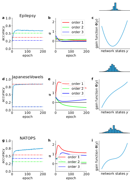
FIG. 6: Training on a few example benchmark datasets. Training progress and final gain function in the OSP for Epilepsy (a - c), JapaneseVowels (d - f) and NATOPS (g - i) datasets, respectively. Accuracy of the full network (blue curve) and single-order accuracy at the end of training for orders one (red), two (green), and three (blue) as horizontal lines (left). Evolution of cumulant combination weights $\alpha$ (middle). Gain function $\phi(y)$ resulting from final $\alpha$, including the density of samples in the domain.

As a next step, we train and benchmark the OSP on $18$ datasets previously used for benchmarking of time-series classification [10]. They consist of multivariate time series with a diversity of input dimensionalities, durations and sample sizes, as well as number of classes. Fig. 6 displays the classification results of the OSP for selected datasets that have different statistical structures. For the example in Fig. 6 (g-i), a large synergy from combining mostly the first and third order evolves in the first few epochs. Decoding on individual statistical orders, an accuracy of $53\,\%$ is achieved for the mean, $32\,\%$ for the covariance, and $42\,\%$ for the third order. The total classification accuracy combining all orders reaches $75\,\%$. As we quantify synergy by the difference between the final accuracy and the largest single order accuracy, this corresponds to a synergy of $+22\,\%$.

The optimal gain function corresponding to this statistical structure is consequently nearly point symmetric. The fluctuations of the samples mostly pass through the region close to the origin. Only some classes operate in the regime of strong non-linearity. Fig. 6 (a-c) and Fig. 6 (d-f) show similar results for the Epilepsy and JapaneseVowels dataset, respectively. Here, the optimal gain functions are mostly quadratic or linear, respectively.

FIG. 7: Classification results on empirical datasets. (a) Comparison of the accuracy achieved in the ML and OSP models. Colors indicate the datasets as listed on the side. (b) Analogous to (a) with a constrained ML model with as many trainable parameters as the OSP. (c) Synergy (see Section II.1.4) of the OSP for different datasets. Size and opacity indicate the improvement in classification accuracy as compared to the pre-training accuracy (larger size and more contrast for larger improvement).

In Fig. 7 (a), we compare the performance of the benchmark datasets of the OSP to the ML model. Our goal is less to compare to the state of the art with a perceptron-like model (see [57] for recent results), but to showcase how appropriate processing of statistical information can improve network capabilities. Nevertheless, the performance of the OSP often approaches that of the corresponding machine learning model. In most of the cases, both OSP and ML perform above chance level, which we empirically evaluate using similar architectures with untrained parameters. Accuracy remains at chance level only for two datasets: HeadMovementDirection and SelfRegulationSCP2.

For synthetic data (Fig. 4), the OSP yielded mostly lower classification accuracy compared to the ML approach, but outperformed a constrained ML model in which the number of trainable parameters equals those of the OSP. We observe the same for the benchmark datasets in Fig. 7: In comparison to the constrained ML model, we typically find a significant performance increase (see Fig. 7 (b)), whereas the ML model that trains directly on the full input cumulants exhibits even higher performance (see Fig. 7 (a)).

We furthermore extract also the relevant statistical orders in the data by inspecting the trained values of $\alpha$. With the coloring of each dataset according to its cumulant combination weights $\alpha=(\alpha_{1},\alpha_{2},\alpha_{3})=(\text{red},\text{green},\text{blue})$, the broad color spectrum displayed in Fig. 7 shows a wide variety for the relevant statistical orders in the different datasets.

In Fig. 7 (c), we display the accuracy increase with respect to the best single order for the different datasets. While the color indicates the dataset, both size and transparency encode the training performance of the OSP in relation to the pre-training accuracy. Datasets that are less well classified by the OSP are thus displayed smaller and more transparent. Based on the synthetic data, we expect larger synergy where different orders are combined more strongly. In Fig. 7 (c), we therefore relate synergy to the participation ratio $\rho$ (see Section II.1.4). Although the results on synthetic data suggest a non-uniform weighting between the different orders $n$, we observe synergy effects also in complex datasets, specifically from combining more than one statistical order. In this figure, we observe a correlation between the participation ratio and the observed synergy in the different datasets.

IV Discussion

In this work, we analyzed statistical processing for time series by a perceptron-like model with a tuneable non-linearity. We showed that the form of the non-linearity determines which statistical patterns, quantified via cumulants up to the third order, are transformed to shape the network output, and how the different orders jointly contribute to the output to solve the task. The gain function that is optimal for the time series classification tasks depends sensitively on the relative importance of class-specific differences (or contrasts) in each cumulant. With the order selective perceptron, informative statistical properties of the data can be revealed with minimal model complexity.

This minimal complexity is achieved by avoiding the explicit computation of cumulants at several orders. Instead, the selection of the relevant cumulants of the input $x^{t}$, via those of the intermediate variable $y^{t}$, results from the combination of learning rules for the input weights and the nonlinearity. While the input cumulants, in particular the higher orders, require huge tensors for $N$-dimensional multivariate time series with large $N$, the cumulants of $y^{t}$ scale polynomially with $M$, the number of classes, which is already often lower. Since additionally, only the diagonal of the network state cumulant is computed, the computational cost reduces further to only $M$ entries per order. Furthermore, the number of trainable parameters reduces from $K+M\cdot(N+N^{2}+\ldots+N^{K})$ for the ML network to $K+M\cdot N$ for the OSP (with $K$ the maximum cumulant order).

Naturally, this reduced model complexity comes at lower performance, as compared to the explicit computation of all cumulant orders. However, the network layer $B$ practically accumulates as much “information” as possible from the input cumulants in the intermediate variables for classification: We have showed that the OSP performs in between the ML model acting on the same cumulants as the OSP and the constrained ML network, which trains only a reduced set of weights of the original ML architecture (to match the trained parameters of the OSP). The original ML network thereby acts as a theoretical upper bound for the OSP, as it can freely combine all of the input cumulants. The fact that the OSP outperforms the constrained ML model shows the efficient computation in the OSP despite the competition between the different orders. For neural classifiers that perform at the current state of the art, this may suggest as a metric their flexibility with regard to the adaptive propagation of cumulants. For example, in the spirit of [40] which have showed superior performance of covariance encoding in reservoir computing compared to linear encoding, an order selective perceptron could be combined with a recurrent reservoir to combine the benefits of both. A thorough study of more sophisticated, large-scale architectures that utilize high order cumulants in this regard remains for future work.

The regularization-induced competition between the orders in fact strongly affects how the OSP combines cumulants for classification. We created synthetic data with tuneable cumulant structure to investigate this dependence in detail. Our SDE-based algorithm generates data with known cumulants up to third order. Field theory can be used to obtain both estimates of the higher order structures and more accurate estimates of the cumulants, which are given by a series of coefficients with decreasing weights. It is, however, limited to statistics that does not deviate too strongly from the exactly solveable Gaussian theory. To the best of our knowledge, there has to date been no algorithm that would provide the desired controlled data for multivariate time series. It is noteworthy, though, that there exists the CuBIC technique [63, 64], which creates spike trains with a given a desired cumulant structure. The algorithm presented here can also be used to create static stimuli.

Using such synthetic data with known underlying statistical structure, we found that the OSP preferentially classifies using only a single order, relying on only one cumulant, if the difference between the classes is more expressed in this cumulant than in the others. This is reinforced by the regularization of the cumulant combining layer, although the same behavior qualitatively also occurs for unconstrained $\alpha$. In that case, however, the network is classifying a bit less well overall. On the boundary between two different preferred orders, we observe synergy effects from combining cumulants through different paths. The class contrast where this boundary occurs appears however non-trivial. From both the position of the boundary and the amplitudes of the order selection parameter $\alpha$ in the regions next to the boundary, we conclude that the network tends to prefer lower order cumulants over higher ones, and selects the preferred order using this hierarchy. Applied to real-world applications that serve as benchmark datasets, often several orders are combined, and we regularly observe synergistic effects. Combination of statistical information appears all the more important for complicated data structures. For any combination of orders, there is a dataset found among them whose order selection parameters filter for just this combination. The gain functions that the order combination parameters translate to are consequently uniquely shaped.

Neuronal network architectures similar to the OSP have been widely used for different purposes in the context of machine learning [8] and computational neuroscience [62, 59, 15], with nonlinear neurons governed by bounded sigmoid-like profiles like in the Wilson-Cowan-model [69, 70], or rectified linear units (ReLU) [45]. [55] give a thorough review of different gain functions and their influence on computational performance. We stress that our study differs from the use of fixed (non-trainable) gain functions that are typically used. The choice of the gain function, however, matters for the the statistical processing performed by the network. The purely linear gain function corresponds to the original perceptron [54, 44, 68] where each input cumulant is mapped to its counterpart at the same order in the output. In contrast, a nonlinear readout can perform cross-talk between input cumulants of several orders, combining them into e.g. the output mean. On the other hand, correlation patterns have recently been proposed as the basis of “information” embedded in time series that can be processed for e.g. classification [24]. This so-called covariance (de)coding has been shown to yield larger pattern capacity than the classical perceptron that relies on mean patterns when applied to time series [12].

In conclusion, the choice of the gain function at the same time is a choice on what statistical information the network should be sensitive to. Gain functions that are more complex than simple polynomials thus combine many, if not all, orders of cumulants. We chose a polynomial here for interpretability, in practice high performance could be achieved by other choices of tuneable non-linearities. However, a fixed gain function means also that there is a fixed relation between the different statistical contributions of the underlying probability density. Translating a given gain function into a Taylor series around a working point can give insight into what cumulants a network may be particularly sensitive to, although this does not yield a one-to-one translation to our adaptive gain function. The here employed de-meaning of the time series translates to a different weighting of cumulants depending on the sample’s mean; it still holds that this form of input processing is fixed and pre-defined. In biological data, adaptive gain has been observed [14, 43], although not identical to the simple mechanism presented here.

We therefore suggest making the choice of gain function with care. There have been, in fact, works on comparing how well different prominent gain functions work in machine learning contexts [48, 66], and some commonly used gain functions include trainable parameters [39]. A fully trainable gain function is presented in [16], which is of a similar polynomial type as presented here. The aim of these works is to provide optimal performance for sophisticated networks on complicated tasks. We offer interpretability of the gain function in terms of statistical processing and provide a link to biological neural networks.

The gain variability found for example by [14, 43] shows that neurons may be sensitive to the statistical features of their inputs, and the variability of activity also appears to be linked to behavior [52, 38, 60]. It may also play a role in representing uncertainty in terms of probabilistic inference [6, 49, 30, 17]. Structured variability thus seems to play an integral role in biological neural networks. As far as information encoding through neural correlations is superior to mean-based representations, this may help understand why such sensitivity has emerged in neuronal circuits. This reasoning has already inspired the covariance perceptron [23, 12].

Of course, just like the covariance perceptron, the order selective perceptron is not a biologically detailed network model. It is built upon the most fundamental building block, a feedforward layer of neurons, followed by a gain function. Instead of individual neuron’s spiking activity, it treats populations of neurons as a unit with an activity that resembles the average firing rate. The linear summation of inputs resembles closely the neuron dynamics typically assumed for cortical models [62, 3, 51, 31, 37], but also in machine learning, including the perceptron [54, 44, 68]. The main difference to previously presented methods is the assumption of information being hidden in the higher order statistics of the network activity. While the propagation of stimuli through neural networks is widely accepted to be modeled suitably by linear summation of inputs and application of subsequent transfer functions, this point of view draws more towards understanding the computation based on the inputs.

Both regarding computational capacity and biological realism, it would be interesting to study also a multi-layer or a recurrently connected version of the order selective perceptron, which extends outside the scope of this work. It is of particular relevance to study the performance gain from time-lagged cumulants. Further, the cross-correlations of the intermediate network state, which are currently not influencing the classification, may be useful in future work.

APPENDIX A Computation of cumulants for the artificial data model

The cumulants of the probability density $p(x)\sim\exp\left(-\beta\left(m^{T}x+\frac{1}{2}x^{T}Jx+\frac{1}{3!}\sum_{ijk}K_{ijk}x_{i}x_{j}x_{k}\right)\right)$ (with a potential barrier) can be derived using field theory [29]. To this end, the Gaussian model with $p(x)\sim\exp\left(-\beta\left(m^{T}x+\frac{1}{2}x^{T}Jx\right)\right)$ acts as a baseline, and the cubic part forms a small correction for states near those expected from the Gaussian distribution. From the Gaussian baseline follows, that the propagator of the system is its covariance,

$$\Sigma_{ij}=\frac{1}{\beta}(J^{-1})_{ij}\,.$$ (23)

With $m$ acting as a source term, the mean follows as

$$\mu_{i}=-\sum_{j}(J^{-1})_{ij}m_{j}\,.$$ (24)

The cubic correction leads to a three-point vertex, which has the value $-\frac{\beta}{3!}K$. In first order corrections to the Gaussian theory, therefore, diagrams with a single vertex need to be computed. For the mean, this leads to a tadpole diagram, where two of the three legs of a vertex are connected by the propagator, and a single external leg. There are three different such diagrams from the three possible choices of the external legs, leading to the corrected mean

$$\mu_{i}=-\sum_{j}(J^{-1})_{ij}m_{j}-\frac{1}{2\beta}\sum_{jkl}(J^{-1})_{ij}K_{jkl}(J^{-1})_{kl}\,.$$ (25)

This mean may not deviate too strongly from the Gaussian one. There are no diagrams with a single three-point vertex and two external legs, so up to first order, the covariance stays as in the Gaussian case. The third order cumulant is simply a vertex with a propagator on each of its legs. A prefactor of $3!$ needs to be included for those. To summarize, this leads to the cumulants

$$\mu_{i} \approx-\sum_{j}(J^{-1})_{ij}m_{j}-\frac{1}{2\beta}\sum_{jkl}(J^{-1})_{ij}K_{jkl}(J^{-1})_{kl}\,,$$ (26)

$$\Sigma_{ij} \approx\frac{1}{\beta}(J^{-1})_{ij}\,,$$ (27)

$$S_{ijk} \approx-\frac{1}{\beta^{2}}\sum_{i^{\prime}j^{\prime}k^{\prime}}K_{i^{\prime}j^{\prime}k^{\prime}}(J^{-1})_{ii^{\prime}}(J^{-1})_{jj^{\prime}}(J^{-1})_{kk^{\prime}}\,.$$ (28)

APPENDIX B How to choose suitable parameters

In order to obtain reasonable results, the parameters need to be chosen with care. The cubic part $K$ may not be too large, to ensure the system is both not too unstable and close enough to the Gaussian case that we can use field theory to approximate the cumulant statistics, however large enough that substantial third order statistics arises for our desired dataset. To this end, we compare the expected fluctuations of states with the width of the safe part of the potential, the region between the local minimum and the local maximum.

For this comparison to be useful, however, we first need to ensure that during all times of the evolution of the SDE, the data stays close to the Gaussian theory. Therefore, we simulate the SDE with random initial conditions drawn from a Gaussian distribution with mean and covariance identical to those expected according to Section A. Furthermore, we set the source $m=0$ to simplify calculations. The mean of the data can anyway be adjusted by a constant shift $b$ of all data points after simulating the SDE. The quadratic part $J$ needs to be chosen as a positive definite matrix that fits the desired covariance.

The remaining parameter to determine is therefore only $K$. It has to be chosen such that for $m=0$ and a given $J$, there is no direction of the potential where the Lagrangian $L[x]=\frac{1}{2}x^{T}Jx+\frac{1}{3!}\sum_{ijk}K_{ijk}x_{i}x_{j}x_{k}$ rises monotonically. For a start, we’ll assume that the cubic part will be of rank one, in the sense that there is a single direction in state space where the Lagrangian is cubic, and in all directions orthogonal to this one, the potential remains quadratic. We’ll be then able to compose stronger cubic potentials.

With $x^{\prime}$ in direction of non-vanishing cubic interactions, this means that there must be real solutions to the necessary conditions for local minima or maxima,

$$\sum_{j}J_{ij}x_{j}^{\prime}+\frac{1}{2}\sum_{jk}K_{ijk}x_{j}^{\prime}x_{k}^{\prime}=0\,.$$ (29)

Only then, a stable region will exist for the data to evolve around. With $K$ being rank one, it can be composed as an outer product of vectors $v$ as

$$K_{ijk} =v_{i}v_{j}v_{k}\,.$$ (30)

The condition for local extrema becomes

$$Jx^{\prime}+\frac{1}{2}v(v^{T}x{}^{\prime})^{2}=0\,.$$ (31)

As desired, in any direction orthogonal to $v$ (i.e. where $v^{T}x{}^{\prime}=0$), then the potential is quadratic and thereby stable. It therefore suffices to look at $x^{\prime}\parallel v$. In that case, when $x^{\prime}=\|x\|e^{(\!v\!)}$,

$$Jx^{\prime}+\frac{1}{2}v(v^{T}x{}^{\prime})^{2} =\|x\|Je^{(\!v\!)}+\frac{1}{2}\|x\|^{2}\,\|v\|^{3}\>e^{(\!v\!)}$$ (32)

$$=0$$ (33)

where $e^{(\!v\!)}$ denotes the unit vector in direction of $v$. If $e^{(\!v\!)}$ is an eigendirection of $J$ with eigenvalue $\lambda_{(\!v\!)}$, this simplifies further. Then, one can solve for $\|v\|$ to obtain $v=\|v\|\>e^{(\!v\!)}=-2^{\frac{1}{3}}\|x\|^{-\frac{1}{3}}\lambda_{(\!v\!)}^{\frac{1}{3}}\>e^{(\!v\!)}$. Now, the extrema of the potential lie on a line in direction $e^{(\!v\!)}$, at $x^{\prime}=0$ and $x^{\prime}=\|x\|e^{(\!v\!)}$. The distance between the minimum and maximum therefore is $\|x\|$ and can be chosen to determine the cubic part of the Lagrangian. We can here choose to set

$$\|x\|^{2}=s^{2}e^{(\!v\!)\mathrm{T}}\Sigma e^{(\!v\!)}$$ (34)

such that we expect $s$ standard deviations to fit in this stable part of the potential (see Section A).

We can lastly compare the third order cumulant to the second to find values of $s$ for the third order statistics to be strong enough compared to the fluctuations. To this end, we can map the second and third order statistics in some eigendirection $e^{(\!v^{\prime}\!)}$ of $J$ (which is also an eigendirection of $\Sigma$ with eigenvalue $(\beta\lambda_{v^{\prime}})^{-1}$) to find

$$\left(e^{(\!v^{\prime}\!)\mathrm{T}}\Sigma e^{(\!v^{\prime}\!)}\right)^{\frac{3}{2}}=\left(\beta\lambda_{(\!v^{\prime}\!)}\right)^{-\frac{3}{2}}$$ (35)

and

$$\sum_{ijk}S_{ijk}e_{i}^{(\!v^{\prime}\!)}e_{j}^{(\!v^{\prime}\!)}e_{k}^{(\!v^{\prime}\!)} =-\frac{1}{\beta^{2}}\left(e^{(\!v^{\prime}\!)\mathrm{T}}J^{-1}v\right)^{3}$$

$$=-\frac{1}{\beta^{2}}\left(e^{(\!v^{\prime}\!)}\lambda_{(\!v\!)}^{-1}v\right)^{3}$$

$$=-\frac{\|v\|^{3}}{\beta^{2}\lambda_{(\!v\!)}^{3}}\delta_{vv^{\prime}}$$

$$=\frac{1}{\|x\|\beta^{2}\lambda_{(\!v\!)}^{2}}\delta_{vv^{\prime}}$$

$$=\frac{1}{s\left(e^{(\!v\!)\mathrm{T}}\Sigma e^{(\!v\!)}\right)^{\frac{1}{2}}\beta^{2}\lambda_{(\!v\!)}^{2}}\delta_{vv^{\prime}}$$

$$=\frac{1}{s}\left(\beta\lambda_{(\!v\!)}\right)^{-\frac{3}{2}}\delta_{vv^{\prime}}.$$ (36)

From this follows

$$\left|\frac{\sum_{ijk}S_{ijk}e_{i}^{(\!v\!)}e_{j}^{(\!v\!)}e_{k}^{(\!v\!)}}{\left(\sum_{ij}\Sigma_{ij}e_{i}^{(\!v\!)}e_{j}^{(\!v\!)}\right)^{\frac{3}{2}}}\right|=\frac{1}{s}$$ (37)

for $e^{(\!v\!)}$ in direction of the cubic perturbation.

It is straightforward to then construct a Lagrangian with a safe cubic potential in any direction by summing over all eigendirections of $J$,

$$K_{ijk} =\sum_{(\!v\!)}v_{i}^{(\!v\!)}v_{j}^{(\!v\!)}v_{k}^{(\!v\!)}\,,$$ (38)

$$v^{(\!v\!)} =-s_{(\!v\!)}^{-\frac{1}{3}}\left(e^{(\!v\!)T}\Sigma e^{(\!v\!)}\right)^{-\frac{1}{6}}\lambda_{(\!v\!)}^{\frac{1}{3}}\>e^{(\!v\!)}\,,$$ (39)

where $s_{(\!v\!)}$ controls the strength of the cubic potential in each eigendirection of $J$. For or purposes, $s=s_{(\!v\!)}=3$ was used in all directions.

APPENDIX C Comparison to constrained order perceptron models

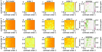
FIG. 8: Performance comparison of the OSP and a constrained OSP. (a) Accuracy of the OSP as in Fig. 3. (b) Accuracy of a constrained OSP with trainable $\alpha_{1}$ and $\alpha_{2,3}=0$. (c, d) Analogous to (b) with $\alpha_{2,3}$ trainable, respectively. (e) Accuracy gain of the OSP over the constrained OSP. In (a - e), classes are separated by a difference in the mean and covariance. In (f - j), classes are separated by a difference in the mean and third order cumulant. In (k - o), classes are separated by a difference in the covariance and third order cumulant.

We defined synergy as the performance gain of the OSP compared to a pruned OSP, where all except a single entry of $\alpha$ is set to zero. This is motivated by the ability of $\alpha$ to indicate the contribution of corresponding statistical orders to the classification decision, as deduced from the competition between its entries. A different angle to the question of how much the OSP gains can be whether and when the OSP outperforms a constrained OSP, in which entries of $\alpha$ are set to zero throughout training.

Fig. 8 shows a comparison of the performance of these models. Constrained OSP ignore the contrasts in cumulants that they are not sensitive to and perform well above a minimum contrast in their corresponding cumulant order. Without the competition imposed on the unconstrained OSP, the performance is typically higher than the single order accuracy given by the pruned networks in Fig. 3. Consequently, the difference of accuracy between these models is lower. However, we still observe a tendency towards an accuracy gain along an area in the space of contrasts. Noticeably, it coincides mostly with the border between areas in which individual orders dominate the unconstrained OSP (see Fig. 3). The OSP therefore actively benefits from combining different cumulants for classification.

APPENDIX D Synthetic data, ML model

Training of the ML network on the synthetic data is displayed in Fig. 9. In Fig. 10, the training is repeated with an ML model, of which only $MN$ weights are randomly selected to be trainable.

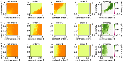
FIG. 9: Readout parameters for the ML network with varying task difficulties. Datasets with two equal-sized classes which differ in two of their first three cumulants (rows) are classified using the ML network. The cumulant combination weight $\alpha$ is displayed for the full model (left) in color code, for the first (red), second (green) and third order (blue). Insets show the corresponding gain function at different points of the parameter regime for the OSP. Consecutively, starting from the second from left, $\alpha_{i}$ for each individual order $i$ from one (mean) to three (third order cumulant) is showed. The axes of each diagram display the contrast between the classes underlying the datasets, starting from one (no class difference) to an arbitrarily chosen upper scale. In (a - e), classes are separated by a difference in the mean and covariance. In (f - j), classes are separated by a difference in the mean and third order cumulant. In (k - o), classes are separated by a difference in the covariance and third order cumulant.

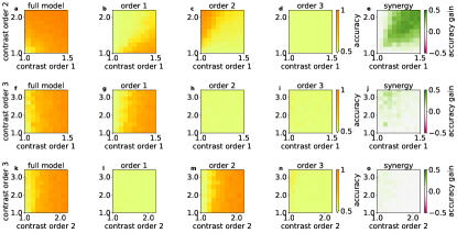
FIG. 10: Readout parameters for the constrained ML model with varying task difficulties. Datasets with two equal-sized classes which differ in two of their first three cumulants (rows) are classified using the constrained ML network. The cumulant combination weight $\alpha$ is displayed for the full model (left) in color code, for the first (red), second (green), and third order (blue). Insets show the corresponding gain function at different points of the parameter regime for the OSP. Consecutively, starting from the second from left, $\alpha_{i}$ for each individual order $i$ from one (mean) to three (third order cumulant) is showed. The axes of each diagram display the contrast between the classes underlying the datasets, starting from one (no class difference) to an arbitrarily chosen upper scale. In (a - e), classes are separated by a difference in the mean and covariance. In (f - j), classes are separated by a difference in the mean and third order cumulant. In (k - o), classes are separated by a difference in the covariance and third order cumulant.

References

- Abraham [2008] Wickliffe C Abraham. Metaplasticity: tuning synapses and networks for plasticity. Nature Reviews Neuroscience, 9(5):387–387, 2008.
- Alzubaidi et al. [2021] Laith Alzubaidi, Jinglan Zhang, Amjad J Humaidi, Ayad Al-Dujaili, Ye Duan, Omran Al-Shamma, José Santamaría, Mohammed A Fadhel, Muthana Al-Amidie, and Laith Farhan. Review of deep learning: Concepts, cnn architectures, challenges, applications, future directions. Journal of big Data, 8(1):1–74, 2021.
- Amari [1972] Shun-Ichi Amari. Characteristics of random nets of analog neuron-like elements. SMC-2(5):643–657, 1972. ISSN 2168-2909. doi: 10.1109/TSMC.1972.4309193.
- Arieli et al. [1996] A. Arieli, A. Sterkin, A. Grinvald, and A. Aertsen. Dynamics of ongoing activity: explanation of the large variability in evoked cortical responses. 273(5283):1868–1871, 1996.
- Bagnall et al. [2017] Anthony Bagnall, Jason Lines, Aaron Bostrom, James Large, and Eamonn Keogh. The great time series classification bake off: a review and experimental evaluation of recent algorithmic advances. 31(3):606–660, 2017.
- Berkes et al. [2011] Pietro Berkes, Gergő Orbán, Máté Lengyel, and József Fiser. Spontaneous cortical activity reveals hallmarks of an optimal internal model of the environment. 331(6013):83–87, jan 2011. doi: 10.1126/science.1195870. URL https://doi.org/10.1126%2Fscience.1195870.
- Bienenstock et al. [1982] Elie L. Bienenstock, Leon N. Cooper, and Paul W. Munro. Theory for the development of neuron selectivity: orientation specificity and binocular interaction in visual cortex. 2(1):32–48, 1982.
- Can and Krishnamurthy [2021] Tankut Can and Kamesh Krishnamurthy. Emergence of memory manifolds. arXiv preprint arXiv:2109.03879, 2021.
- Caporale and Dan [2008] Natalia Caporale and Yang Dan. Spike timing–dependent plasticity: A hebbian learning rule. 31(1):25–46, July 2008. doi: 10.1146/annurev.neuro.31.060407.125639. URL https://doi.org/10.1146/annurev.neuro.31.060407.125639.
- Chen et al. [2015] Yanping Chen, Eamonn Keogh, Bing Hu, Nurjahan Begum, Anthony Bagnall, Abdullah Mueen, and Gustavo Batista. The ucr time series classification archive. 2015. URL https://www.cs.ucr.edu/~eamonn/time_series_data_2018/.
- Cho et al. [2014] Kyunghyun Cho, Bart van Merriënboer, Dzmitry Bahdanau, and Yoshua Bengio. On the properties of neural machine translation: Encoder–decoder approaches. In Proceedings of SSST-8, Eighth Workshop on Syntax, Semantics and Structure in Statistical Translation, pages 103–111, 2014.
- Dahmen et al. [2020] David Dahmen, Matthieu Gilson, and Moritz Helias. Capacity of the covariance perceptron. 53(35):354002, aug 2020. doi: 10.1088/1751-8121/ab82dd. URL https://doi.org/10.1088%2F1751-8121%2Fab82dd.
- DePasquale et al. [2018] Brian DePasquale, Christopher J Cueva, Kanaka Rajan, G Sean Escola, and LF Abbott. full-force: A target-based method for training recurrent networks. 13(2), 2018.
- Díaz-Quesada and Maravall [2008] Marta Díaz-Quesada and Miguel Maravall. Intrinsic mechanisms for adaptive gain rescaling in barrel cortex. Journal of Neuroscience, 28(3):696–710, 2008.
- Engelken et al. [2022] Rainer Engelken, Alessandro Ingrosso, Ramin Khajeh, Sven Goedeke, and L. F. Abbott. Input correlations impede suppression of chaos and learning in balanced rate networks. 2022. URL https://arxiv.org/abs/2201.09916.
- Ertuğrul [2018] Ömer Faruk Ertuğrul. A novel type of activation function in artificial neural networks: Trained activation function. Neural Networks, 99:148–157, 2018.
- Festa et al. [2021] Dylan Festa, Amir Aschner, Aida Davila, Adam Kohn, and Ruben Coen-Cagli. Neuronal variability reflects probabilistic inference tuned to natural image statistics. Nature communications, 12(1):1–11, 2021.
- Fries [2015] Pascal Fries. Rhythms for cognition: communication through coherence. Neuron, 88(1):220–235, 2015.
- Fuchs et al. [2009] Erich Fuchs, Christian Gruber, Tobias Reitmaier, and Bernhard Sick. Processing short-term and long-term information with a combination of polynomial approximation techniques and time-delay neural networks. IEEE Transactions on Neural Networks, 20(9):1450–1462, 2009.
- Gardiner [1985] Crispin W. Gardiner. Handbook of Stochastic Methods for Physics, Chemistry and the Natural Sciences. Number 13 in Springer Series in Synergetics. Springer-Verlag, Berlin, 2nd edition, 1985. ISBN 3-540-61634-9, 3-540-15607-0.
- Gerstner et al. [1996] Wulfram Gerstner, Richard Kempter, J. Leo van Hemmen, and Hermann Wagner. A neuronal learning rule for sub-millisecond temporal coding. 383:76–78, September, 5 1996.
- Gilson et al. [2011] Matthieu Gilson, Timothée Masquelier, and Etienne Hugues. Stdp allows fast rate-modulated coding with poisson-like spike trains. PLoS computational biology, 7(10):e1002231, 2011.
- Gilson et al. [2019] Matthieu Gilson, David Dahmen, Ruben Moreno-Bote, Andrea Insabato, and Moritz Helias. The covariance perceptron: A new framework for classification and processing of time series in recurrent neural networks. 2019. doi: 10.1101/562546. 562546.
- Gilson et al. [2020] Matthieu Gilson, David Dahmen, Rubén Moreno-Bote, Andrea Insabato, and Moritz Helias. The covariance perceptron: A new paradigm for classification and processing of time series in recurrent neuronal networks. 16(10):1–38, 10 2020. doi: 10.1371/journal.pcbi.1008127. URL https://doi.org/10.1371/journal.pcbi.1008127.
- Gjorgjieva et al. [2011] Julijana Gjorgjieva, Claudia Clopath, Juliette Audet, and Jean-Pascal Pfister. A triplet spike-timing–dependent plasticity model generalizes the bienenstock–cooper–munro rule to higher-order spatiotemporal correlations. Proceedings of the National Academy of Sciences, 108(48):19383–19388, 2011.
- Goldenfeld [1992] Nigel Goldenfeld. Lectures on phase transitions and the renormalization group. Perseus books, Reading, Massachusetts, 1992.
- Gütig and Sompolinsky [2006] Robert Gütig and Haim Sompolinsky. The tempotron: a neuron that learns spike timing-based decisions. 9(3):420–428, Mar 2006.
- Hebb [1949] D. O. Hebb. The organization of behavior: A neuropsychological theory. John Wiley & Sons, New York, 1949.
- Helias and Dahmen [2019] Moritz Helias and David Dahmen. Statistical field theory for neural networks. 2019. 1901.10416 [cond-mat.dis-nn].
- Hénaff et al. [2020] Olivier J Hénaff, Zoe M Boundy-Singer, Kristof Meding, Corey M Ziemba, and Robbe LT Goris. Representation of visual uncertainty through neural gain variability. Nature communications, 11(1):1–12, 2020.
- Hermann and Touboul [2012] Geoffroy Hermann and Jonathan Touboul. Heterogeneous connections induce oscillations in large-scale networks. 109(1):018702, 2012.
- Hertz et al. [1991] John Hertz, Anders Krogh, and Richard G. Palmer. Introduction to the Theory of Neural Computation. Perseus Books, 1991. ISBN 0-201-51560-1.
- Hochreiter and Schmidhuber [1997] Sepp Hochreiter and Jürgen Schmidhuber. Long short-term memory. 9(8):1735–1780, 1997.
- Hochreiter et al. [2001] Sepp Hochreiter, Yoshua Bengio, Paolo Frasconi, Jürgen Schmidhuber, et al. Gradient flow in recurrent nets: the difficulty of learning long-term dependencies, 2001.
- Izhikevich and Desai [2003] Eugene M. Izhikevich and Niraj S. Desai. Relating STDP to BCM. 15:1511–1523, 2003.
- Jaeger [2001] H. Jaeger. The “echo state” approach to analysing and training recurrent neural networks. Technical Report GMD Report 148, German National Research Center for Information Technology, St. Augustin, Germany, 2001.
- Kadmon and Sompolinsky [2015] Jonathan Kadmon and Haim Sompolinsky. Transition to chaos in random neuronal networks. page 1508.06486, 2015.
- Kilavik et al. [2009] Bjørg E Kilavik, Sébastien Roux, Adrián Ponce-Alvarez, Joachim Confais, Sonja Grün, and Alexa Riehle. Long-term modifications in motor cortical dynamics induced by intensive practice. 29(40):12653–12663, 2009.
- Lau and Lim [2018] Mian Mian Lau and King Hann Lim. Review of adaptive activation function in deep neural network. In 2018 IEEE-EMBS Conference on Biomedical Engineering and Sciences (IECBES), pages 686–690. IEEE, 2018.
- Lawrie et al. [2021] Sofía Lawrie, Rubén Moreno-Bote, and Matthieu Gilson. Covariance-based information processing in reservoir computing systems. bioRxiv, 2021.
- LeCun et al. [2015] Yann LeCun, Yoshua Bengio, and Geoffrey Hinton. Deep learning. 521(7553):436–444, 2015.
- Maass et al. [2002] Wolfgang Maass, Thomas Natschläger, and Henry Markram. Real-time computing without stable states: a new framework for neural computation based on perturbations. 14(11):2531–2560, 2002.
- Maravall et al. [2013] Miguel Maravall, Andrea Alenda, Michael R Bale, and Rasmus S Petersen. Transformation of adaptation and gain rescaling along the whisker sensory pathway. PLoS One, 8(12):e82418, 2013.
- Minsky and Papert [1969] M L Minsky and S A Papert. Perceptrons. Cambridge MIT Press, 1969.
- Nair and Hinton [2010] Vinod Nair and Geoffrey E Hinton. Rectified linear units improve restricted boltzmann machines. In Icml, 2010.
- Nauhaus et al. [2009] Ian Nauhaus, Laura Busse, Matteo Carandini, and Dario L. Ringach. Stimulus contrast modulates functional connectivity in visual cortex. 12:70–76, 2009. doi: 10.1038/nn.2232. URL https://doi.org/10.1038/nn.2232.
- Nestler et al. [2020] Sandra Nestler, Christian Keup, David Dahmen, Matthieu Gilson, Holger Rauhut, and Moritz Helias. Unfolding recurrence by Green’s functions for optimized reservoir computing. In Advances in Neural Information Processing Systems, volume 33, pages 17380–17390, 2020. URL https://proceedings.neurips.cc/paper/2020/file/c94a589bdd47870b1d74b258d1ce3b33-Paper.pdf.
- Nwankpa et al. [2018] Chigozie Nwankpa, Winifred Ijomah, Anthony Gachagan, and Stephen Marshall. Activation functions: Comparison of trends in practice and research for deep learning. arXiv preprint arXiv:1811.03378, 2018.
- Orbán et al. [2016] Gergő Orbán, Pietro Berkes, József Fiser, and Máté Lengyel. Neural variability and sampling-based probabilistic representations in the visual cortex. 92(2):530–543, oct 2016. doi: 10.1016/j.neuron.2016.09.038. URL https://doi.org/10.1016%2Fj.neuron.2016.09.038.
- Ponulak and Kasiński [2010] Filip Ponulak and Andrzej Kasiński. Supervised learning in spiking neural networks with resume: sequence learning, classification, and spike shifting. Neural computation, 22(2):467–510, 2010.
- Rajan et al. [2010] Kanaka Rajan, LF Abbott, and Haim Sompolinsky. Stimulus-dependent suppression of chaos in recurrent neural networks. 82(1):011903, 2010.
- Riehle et al. [1997a] Alexa Riehle, Sonja Grün, Markus Diesmann, and Ad Aertsen. Spike synchronization and rate modulation differentially involved in motor cortical function. 278(5345):1950–1953, 1997a. doi: 10.1126/science.278.5345.1950.
- Riehle et al. [1997b] Alexa Riehle, Sonja Grün, Markus Diesmann, and Ad Aertsen. Spike synchronization and rate modulation differentially involved in motor cortical function. 278:1950–1953, 1997b.
- Rosenblatt [1958] Frank Rosenblatt. The perceptron: a probabilistic model for information storage and organization in the brain. 65(6):386, 1958.
- Rosenzweig et al. [2020] Jan Rosenzweig, Zoran Cvetkovic, and Ivana Rosenzweig. Goldilocks neural networks. arXiv preprint arXiv:2002.05059, 2020.
- Rubino et al. [2006] Doug Rubino, Kay A. Robbins, and Nicholas G. Hatsopoulos. Propagating waves mediate information transfer in the motor cortex. 9(12):1549–1557, November 2006. doi: 10.1038/nn1802. URL https://doi.org/10.1038/nn1802.
- Ruiz et al. [2021] Alejandro Pasos Ruiz, Michael Flynn, James Large, Matthew Middlehurst, and Anthony Bagnall. The great multivariate time series classification bake off: a review and experimental evaluation of recent algorithmic advances. Data Mining and Knowledge Discovery, 35(2):401–449, 2021.
- Sato et al. [2012] Tatsuo K. Sato, Ian Nauhaus, and Matteo Carandini. Traveling waves in visual cortex. 75(2):218–229, July 2012. doi: 10.1016/j.neuron.2012.06.029. URL https://doi.org/10.1016/j.neuron.2012.06.029.
- Schuecker et al. [2018] Jannis Schuecker, Sven Goedeke, and Moritz Helias. Optimal sequence memory in driven random networks. 8:041029, 2018. doi: 10.1103/PhysRevX.8.041029. URL https://link.aps.org/doi/10.1103/PhysRevX.8.041029.
- Shahidi et al. [2019] Neda Shahidi, Ariana R Andrei, Ming Hu, and Valentin Dragoi. High-order coordination of cortical spiking activity modulates perceptual accuracy. Nature neuroscience, 22(7):1148–1158, 2019.
- Siegle et al. [2021] Joshua H. Siegle, Xiaoxuan Jia, Séverine Durand, Sam Gale, Corbett Bennett, Nile Graddis, Greggory Heller, Tamina K. Ramirez, Hannah Choi, Jennifer A. Luviano, Peter A. Groblewski, Ruweida Ahmed, Anton Arkhipov, Amy Bernard, Yazan N. Billeh, Dillan Brown, Michael A. Buice, Nicolas Cain, Shiella Caldejon, Linzy Casal, Andrew Cho, Maggie Chvilicek, Timothy C. Cox, Kael Dai, Daniel J. Denman, Saskia E. J. de Vries, Roald Dietzman, Luke Esposito, Colin Farrell, David Feng, John Galbraith, Marina Garrett, Emily C. Gelfand, Nicole Hancock, Julie A. Harris, Robert Howard, Brian Hu, Ross Hytnen, Ramakrishnan Iyer, Erika Jessett, Katelyn Johnson, India Kato, Justin Kiggins, Sophie Lambert, Jerome Lecoq, Peter Ledochowitsch, Jung Hoon Lee, Arielle Leon, Yang Li, Elizabeth Liang, Fuhui Long, Kyla Mace, Jose Melchior, Daniel Millman, Tyler Mollenkopf, Chelsea Nayan, Lydia Ng, Kiet Ngo, Thuyahn Nguyen, Philip R. Nicovich, Kat North, Gabriel Koch Ocker, Doug Ollerenshaw, Michael Oliver, Marius Pachitariu, Jed Perkins, Melissa Reding, David Reid, Miranda Robertson, Kara Ronellenfitch, Sam Seid, Cliff Slaughterbeck, Michelle Stoecklin, David Sullivan, Ben Sutton, Jackie Swapp, Carol Thompson, Kristen Turner, Wayne Wakeman, Jennifer D. Whitesell, Derric Williams, Ali Williford, Rob Young, Hongkui Zeng, Sarah Naylor, John W. Phillips, R. Clay Reid, Stefan Mihalas, Shawn R. Olsen, and Christof Koch. Survey of spiking in the mouse visual system reveals functional hierarchy. 592(7852):86–92, Apr 2021. doi: 10.1038/s41586-020-03171-x.
- Sompolinsky et al. [1988] H. Sompolinsky, A. Crisanti, and H. J. Sommers. Chaos in random neural networks. 61:259–262, Jul 1988. doi: 10.1103/PhysRevLett.61.259. URL http://link.aps.org/doi/10.1103/PhysRevLett.61.259.
- Staude et al. [2010a] Benjamin Staude, Sonja Grün, and Stefan Rotter. Higher-order correlations in non-stationary parallel spike trains: statistical modeling and inference. 4, July 2010a. Article nr 16, doi: 10.3389/fncom.2010.00016.
- Staude et al. [2010b] Benjamin Staude, Stefan Rotter, and Sonja Grün. Cubic: cumulant based inference of higher-order correlations in massively parallel spike trains. 29:327–350, 2010b. DOI 10.1007/s10827-009-0195-x.
- Sussillo and Abbott [2009] David Sussillo and Larry F Abbott. Generating coherent patterns of activity from chaotic neural networks. 63(4):544–557, 2009.
- Szandała [2021] Tomasz Szandała. Review and comparison of commonly used activation functions for deep neural networks. In Bio-inspired neurocomputing, pages 203–224. Springer, 2021.
- Waibel et al. [1989] Alexander Waibel, Toshiyuki Hanazawa, Geoffrey Hinton, Kiyohiro Shikano, and Kevin J Lang. Phoneme recognition using time-delay neural networks. IEEE transactions on acoustics, speech, and signal processing, 37(3):328–339, 1989.
- Widrow and Hoff [1960] B Widrow and M E Hoff. Adaptive switching circuits. In IRE, editor, 1960 IRE WESCON Convention Record (Part 4), pages 96–104, 1960.
- Wilson and Cowan [1972] H. R. Wilson and J. D. Cowan. Excitatory and inhibitory interactions in localized populations of model neurons. 12(1):1–24, Jan 1972. doi: 10.1016/s0006-3495(72)86068-5. URL https://doi.org/10.1016/s0006-3495(72)86068-5.
- Wilson and Cowan [1973] H. R. Wilson and J. D. Cowan. A mathematical theory of the functional dynamics of cortical and thalamic nervous tissue. 13(2):55–80, September 1973. doi: 10.1007/bf00288786. URL https://doi.org/10.1007/bf00288786.
- Zenke and Ganguli [2018] Friedemann Zenke and Surya Ganguli. Superspike: Supervised learning in multilayer spiking neural networks. Neural computation, 30(6):1514–1541, 2018.
- Zenke et al. [2015] Friedemann Zenke, Everton J Agnes, and Wulfram Gerstner. Diverse synaptic plasticity mechanisms orchestrated to form and retrieve memories in spiking neural networks. Nature communications, 6(1):1–13, 2015.