Optimal population transfer using the adiabatic rapid passage in the presence of drive-induced dissipation

Abstract

Adiabatic rapid passage (ARP) is extensively used to achieve efficient transfer or inversion of populations in quantum systems. Landau and Zener accurately estimated the transfer probability of ARP for a closed system and showed that this probability improved with higher drive amplitude. Recently, we have found that in open quantum systems, applying a strong drive can give rise to significant drive-induced dissipation (DID). Here, we investigate the effect of DID on the performance of ARP that is implemented using a linearly chirped pulse on a two-level system. From the Landau-Zener formula, the population transfer was known to be enhanced with increasing drive amplitude. However, here we show that beyond a threshold value of the drive amplitude, the transfer probability is reduced because of the detrimental effect of DID. We show that the competition between the two processes results in an optimal behavior of the population transfer. We also propose a phenomenological model that helps explain such nonmonotonic behavior of the transfer. Using this model, we estimate the optimum time at which the maximum population transfer occurs. We extend the analysis for rectangular as well as Gaussian pulse profiles and conclude that a Gaussian pulse outperforms a rectangular pulse.

I Introduction

Adiabatic rapid passage (ARP) is an efficient and robust method for population transfer between two levels of a quantum system. ARP commonly involves applying a chirped pulse across the resonance frequency of two specific energy levels of a quantum system. The chirped pulse, usually symmetric, covers a wide frequency range, with endpoints far away from the resonance. If the sweep is sufficiently slow to satisfy the adiabaticity criterion, then populations of the concerned levels undergo complete inversion with 100% efficiency. In the early 1930s, Landau provided a theoretical description of the process, which Zener perfected soon after Zener (1932); Landau (1932a, b). It is commonly referred to as the Landau-Zener theory since 1970s Matsuzawa (1968); Baede et al. (1969); Olson (1970); Zwally and Cable (1971). According to them, if the adiabaticity criterion is not maintained during the sweep, there is a possibility that the system could make a transition from one eigenstate to the other. This is known as the Landau-Zener (LZ) transition, which is a non-adiabatic transition. So, ARP and LZ transition are two complementary processes and the probability of the population transfer in ARP follows from the LZ formula, as we shall discuss in detail in the next section.

For a linearly chirped drive of constant amplitude $\omega_{1}$ and frequency sweep rate $R$, the adiabaticity condition requires $R/\omega_{1}\ll\omega_{1}$ Abragam (1961). To achieve an efficient transfer, – free from the effects of the environment – the process must be executed fast enough compared to the timescale of relaxation $T_{R}$ of the quantum system. As such, this passage is fast or rapid. The two requirements can be combined as $\frac{1}{T_{R}}\ll\frac{R}{\omega_{1}}\ll\omega_{1}$. The first inequality is the requirement for rapid, whereas the second is the requirement for adiabaticity. So, it is evident that application of higher drive amplitude is preferable for more efficient transfer. This condition also follows from the LZ formula.

As an experimental technique, ARP has been known since its seminal use by Bloch, Hansen, and Packard to detect nuclear magnetic resonance Bloch (1946). Since then, through the works of Redfield, Abragam, Proctor, Slichter, and others, ARP emerged as a useful technique for the population inversion, adiabatic demagnetization, spin temperature studies, and others Drain (1949); Chiarotti et al. (1954); Redfield (1956); Abragam and Proctor (1958); Slichter and Holton (1961); Janzen et al. (1968). In recent times, ARP has been extensively used in population transfer, wavelength conversions, quantum computing, and others Herbers et al. (2022); Kaprálová-Žďánská et al. (2022); Chen et al. (2021); Feilhauer et al. (2020); Mukherjee et al. (2020).

Besides magnetic resonance, ARP has also been used in optical regimes using frequency-swept laser pulses Melinger et al. (1992, 1994); Malinovsky and Krause (2001). Melinger et al. demonstrated that when applied in the adiabatic limit, frequency-swept picosecond laser pulses could be used to achieve efficient population transfer by ARP in two-level and multi-level systems Melinger et al. (1994). A few years later, Malinovsky et al. presented a general theory of ARP with intense, linearly chirped laser pulses Malinovsky and Krause (2001). They derived a modified LZ formula to determine the optimal conditions for efficient and robust population transfer. Maeda et al. reported coherent population transfer between Rydberg states of Li atoms by higher-order multiphoton ARP Maeda et al. (2006). Instead of using a sequence of ARPs of single-photon transitions, they used ARP of a single multiphoton transition.

ARP has also been studied on systems where the “rapid” criterion is not completely satisfied Ao and Rammer (1989, 1991); Ashhab (2016); Nalbach and Thorwart (2009); Wubs et al. (2006); Sun et al. (2016); Whitney et al. (2011). In such systems, the effect of the relaxation on the transfer efficiency is not negligible. Nalbach and others investigated LZ transition in a dissipative environment Nalbach and Thorwart (2009). They showed a non-monotonic dependence of the transition probability on the sweep speed due to competition between relaxation and the external sweep. They explained it in terms of a simple phenomenological model. Sun et al. investigated finite-time LZ processes in the presence of an environment, modeled by a broadened cavity mode at zero temperature Sun et al. (2016). They numerically studied the survival fidelity of adiabatic states. They showed that the fidelity of the transfer exhibits a non-monotonic dependence on the system-environment coupling strength and the sweep rate of the energy bias. Both works hint that the transfer efficiency may be optimal in the case of dissipative dynamics.

We note that a strong chirped pulse favors the ARP condition; the LZ formula of transfer also supports it. For a commonly-employed linearly chirped drive of constant amplitude $\omega_{1}$ and sweep rate $R$, both the conditions imply $\omega_{1}^{2}\gg R$ Abragam (1961). However, we note that a strong drive gives rise to significant excitation-induced dissipation or drive-induced dissipation (DID) in open quantum systems. Although the volume of works mentioned above incorporates the dissipation due to system-environment coupling, they have not considered the drive-induced dissipation. In this work, we incorporate the DID to study the population transfer using ARP in a two-level system (TLS) coupled to its environment. To this end, we use a fluctuation-regulated quantum master equation (FRQME); a recently-proposed Markovian quantum master equation that can estimate the DID Chakrabarti and Bhattacharyya (2018a). We choose the parameters to mimic a nearly-closed system. Thus, for our system, DID is stronger than the relaxation rate processes arising from system-environment coupling. Under this condition, we show that the population transfer has an optimal dependence on $\omega_{1}$. We estimate the critical value and provide a condition for an optimal transfer using a phenomenological model. We propose that in order to achieve the maximum population transfer, we need to stop the drive at that very point of time when the optimal transfer is achieved. If we wait any longer, the transfer will start to decay due to the DID. The analysis has been carried out for two commonly-used pulse profiles- rectangular and Gaussian, and we analyze the relative merits of their use in population transfer.

We organize the remaining part of the manuscript in the following order: In section II, we introduce our frequency sweep model to deal with the problem and describe the mathematical construction of our work. In section III, we show the results. In this section, we also propose a phenomenological model to explain the optimal behavior of population transfer in the presence of DID. In section IV, we discuss the implications of our work. Section V summarizes the major findings and draws final conclusions.

II The model and the method

As is the common practice to emulate ARP, we use a frequency sweep model. We note that Bloch and others originally proposed the feasibility of this process Bloch (1946). In the past, many have used this model to study ARP. Rubbmark et al. used various sweep functions and checked how the energy diagram changes with each sweep Rubbmark et al. (1981). Others have used frequency sweep for efficient population transfer via ARP Melinger et al. (1994); Malinovsky and Krause (2001); Maeda et al. (2006).

Before we add the dissipative effects, we describe the model and its characteristics. We consider a spin-$1/2$ system subjected to a linearly chirped drive swept across the resonance frequency. In the rotating frame of the drive, the Hamiltonian of the system under this process takes the form,

$$H_{\rm\scriptscriptstyle tot}^{*}=-\Delta\omega(t)I_{z}+\omega_{1}I_{x}$$ (1)

where, the frequency offset is taken as, $\Delta\omega(t)=Rt-\delta\omega$, $R=2\delta\omega/T$ is the sweep rate with $T$ being the duration of the sweep, $I_{\alpha}=\sigma_{\alpha}/2$, $\sigma_{\alpha}$ being the Pauli matrix for $\alpha$ component, $\omega_{1}$ is the drive amplitude. In equation (1) and in the subsequent parts, the superscript ‘$*$’ stands for representations in the rotating frame of the drive.

The eigenvalues of the above Hamiltonian are given by,

$$E_{\pm}(t)=\pm\frac{1}{2}\sqrt{(Rt-\delta\omega)^{2}+\omega_{1}^{2}}\>.$$ (2)

The asymptotes for the hyperbola $E_{\pm}(t)$ are as follows,

$$E_{\pm}(t) = \pm\frac{1}{2}(Rt-\delta\omega)=\pm\frac{\Delta\omega(t)}{2}$$ (3)

The figure 1 shows $E_{\pm}(t)$ versus $t$ plot. In this figure, we observe that the energy curves form a set of hyperbolas, and the asymptotes of this hyperbola follow the equation (3). Let us define the asymptotes, $E_{g}=\frac{\Delta\omega(t)}{2}$ and $E_{e}=-\frac{\Delta\omega(t)}{2}$ as the ground state $|g\rangle$ and the excited state $|e\rangle$ energies, respectively.

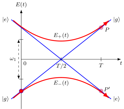
Figure 1: The plot shows the diabats, denoted by blue straight lines (color online) and adiabats, denoted by red hyperbola (color online). For a perfect adiabatic sweep, the system stays on the adiabat. So it can start asymptotically on a diabat $|g\rangle$ at $t=0$ and move adiabatically along the $E_{-}(t)$ adiabat to reach $|e\rangle$ at $t=T$. The Landau-Zener formula gives the transition probability to move from one adiabat to another. The solid red filled circle (color online) depicts a system at state $|g\rangle$ initally. The pale red filled circles (color online) on the adiabats $E_{+}(t)$ and $E_{-}(t)$, at $t=T$ represent the final state of the system with probabilities $P$ and $P^{\prime}$, respectively.

Suppose the system initially lies in the ground state $|g\rangle$ and the perturbing chirped drive is turned on. From figure 1, we can infer the dynamics of the system. In this figure, the red curves that denote the energy eigenvalues $E_{\pm}(t)$ of the total Hamiltonian $H_{\rm\scriptscriptstyle tot}^{*}$, form a hyperbola and are referred to as the adiabats. Since the two energy curves do not cross each other, there is always a minimum gap of $\omega_{1}$ between them, it is called an avoided crossing. The diabats, i.e., the straight blue lines are asymptotes of this hyperbola. They represent the energy eigenvalues of the unperturbed system. In the adiabatic limit $R\ll\omega_{1}^{2}$, the system follows the instantaneous eigenstate and stays in the same adiabat it started in, according to the adiabatic theorem. As a result, the system finally ends up in the other level $|e\rangle$. This demonstrates the use of ARP to transfer the population from one level to the other in a TLS. But if the sweep rate $R$ is very high compared to $\omega_{1}$, i.e. if $R\gg\omega_{1}^{2}$, then the system can make a transition from one energy eigenlevel ($E_{\pm}(t)$) to the other, which is the non-adiabatic Landau-Zener transition.

In our notation, Zener’s formula Zener (1932) for the probability of LZ transition can be expressed as,

$$P=\exp\left(-\frac{\pi\omega_{1}^{2}}{2R}\right).$$ (4)

Therefore, the probability of following the same adiabat would be,

$$P^{\prime}=1-P=1-\exp\left(-\frac{\pi\omega_{1}^{2}}{2R}\right).$$ (5)

In other words, $P^{\prime}$ also indicates the probability of population transfer from one level $|g\rangle$ to the other level $|e\rangle$ using ARP.

II.1 Fluctuation-regulated quantum master equation

In this formulation, we consider a driven quantum system connected to its environment, which is part of a larger heat bath, assumed to be in thermal equilibrium. Further, we consider that this bath experiences thermal fluctuations originating from collisional processes. We describe the system-environment pair by the following Hamiltonian,

$$\mathcal{H}(t)=\mathcal{H}_{\rm\scriptscriptstyle S}^{\circ}+\mathcal{H}_{\rm\scriptscriptstyle E}^{\circ}+\mathcal{H}_{\rm\scriptscriptstyle SE}(t)+\mathcal{H}_{\rm\scriptscriptstyle S}(t)+\mathcal{H}_{\rm\scriptscriptstyle E}(t)$$ (6)

where $\mathcal{H}_{\rm\scriptscriptstyle S}^{\circ}$ is the time-independent Hamiltonian of the system, $\mathcal{H}_{\rm\scriptscriptstyle E}^{\circ}$ is the time-independent Hamiltonian of the environment, $\mathcal{H}_{\rm\scriptscriptstyle SE}(t)$ is the coupling between the system and the environment, $\mathcal{H}_{\rm\scriptscriptstyle S}(t)$ represents the other system Hamiltonians including the external drive applied to the system, and $\mathcal{H}_{\rm\scriptscriptstyle E}(t)$ denotes the fluctuations in the environment. We model the Hamiltonian $\mathcal{H}_{\rm\scriptscriptstyle E}(t)$ as the stochastic fluctuations of the energy levels of $\mathcal{H}_{\rm\scriptscriptstyle E}^{\circ}$, and is chosen to be diagonal in the eigenbasis $\{|\phi_{j}\rangle\}$ of $\mathcal{H}_{\rm\scriptscriptstyle E}^{\circ}$, as represented by, $\mathcal{H}_{\rm\scriptscriptstyle E}(t)=\sum_{j}f_{j}(t)|\phi_{j}\rangle\langle\phi_{j}|$, where $f_{j}(t)$-s are modeled as Gaussian, $\delta$-correlated stochastic variables with zero mean and standard deviation $\kappa$.

The fluctuation-regulated quantum master equation (FRQME) was introduced couple of years back to incorporate the thermal fluctuations of the environment in the dynamics. Chakrabarti and others have provided the complete derivation of the FRQME elsewhere Chakrabarti and Bhattacharyya (2018a); as such, we provide a brief sketch of the derivation. To derive the master equation, one needs to start from the coarse-grained Liouville-von Neumann equation in the interaction representation of $(\mathcal{H}_{\rm\scriptscriptstyle S}^{\circ}+\mathcal{H}_{\rm\scriptscriptstyle E}^{\circ})$ as,

$$\rho_{\rm\scriptscriptstyle S}(t+\Delta t)=\rho_{\rm\scriptscriptstyle S}(t)-i\int_{t}^{t+\Delta t}\kern-22.76219pt\>dt_{1}\kern 5.69054pt{\rm Tr}_{\rm\scriptscriptstyle E}[H_{\rm\scriptscriptstyle eff}(t_{1}),\rho(t_{1})]$$ (7)

where $\rho_{\rm\scriptscriptstyle S}$ denotes the reduced density matrix of the system, $\Delta t$ is the coarse-graining interval, ${\rm Tr}_{\rm\scriptscriptstyle E}$ denotes the partial trace operation on the environmental degrees of freedom, $H_{\rm\scriptscriptstyle eff}(t)=H_{\rm\scriptscriptstyle S}(t)+H_{\rm\scriptscriptstyle SE}(t)$, and $\rho$ is the full density matrix of the system and the environment. We note that the Hamiltonian $\mathcal{H}_{\rm\scriptscriptstyle E}(t)$ is absent in the commutator, because of the partial trace taken over ${\rm E}$. The density matrix inside the commutator at time $t_{1}$ can be written as, $\rho(t_{1})=U(t_{1},t)\rho(t)U^{\dagger}(t_{1},t)$, where $U(t_{1},t)$ denotes the propagator for the system and environment pair from time $t$ to $t_{1}$ in the Hilbert space and is estimated as,

$$U(t_{1},t)\approx U_{\rm\scriptscriptstyle E}(t_{1},t)-i\int_{t}^{t_{1}}H_{\rm\scriptscriptstyle eff}(t_{2})U_{\rm\scriptscriptstyle E}(t_{2})dt_{2}$$ (8)

where $U_{\rm\scriptscriptstyle E}(t_{1},t)$ is a finite propagator for evolution solely under fluctuations, and is given by $\mathcal{T}\exp\left(-i\int_{t}^{t_{1}}dt_{2}\,H_{\rm\scriptscriptstyle E}(t_{2})\right)$, with $\mathcal{T}$ denoting the Dyson time-ordering operator. As such, $U(t_{1},t)$ captures a finite propagation under the environmental fluctuations and an infinitesimal propagation under the system Hamiltonian and the system-environment coupling.

Using the standard Born-Markov and time coarse-graining approximations, we would finally arrive at the following equation,

$$\frac{d}{dt}{\rho_{\rm\scriptscriptstyle S}}(t)= - i\;{\rm Tr}_{\rm\scriptscriptstyle E}[H_{\rm\scriptscriptstyle eff}(t),{\rho_{\rm\scriptscriptstyle S}}(t)\otimes\rho_{\rm\scriptscriptstyle E}^{\rm\scriptscriptstyle eq}]^{\rm sec}$$ (9)

$$- \int_{0}^{\infty}d\tau\;{\rm Tr}_{\rm\scriptscriptstyle E}[H_{\rm\scriptscriptstyle eff}(t),H_{\rm\scriptscriptstyle eff}(t-\tau),{\rho_{\rm\scriptscriptstyle S}}(t)\otimes\rho_{\rm\scriptscriptstyle E}^{\rm\scriptscriptstyle eq}]]^{\rm sec}\;e^{-\frac{|\tau|}{\tau_{c}}}$$

and we call it fluctuation-regulated quantum master equation (FRQME) Chakrabarti and Bhattacharyya (2018a).

In equation (9), we note that $H_{\rm\scriptscriptstyle eff}$ containing the drive as well as the system-environment coupling Hamiltonians, appears in both first- and second-order terms. The drive appearing in the second-order term causes dissipation in the dynamics of the system, which is known as drive-induced dissipation (DID), and has been experimentally verified Chakrabarti and Bhattacharyya (2018b). The environmental fluctuations provide an exponential regulator in the dissipator. In the regulator, $\tau_{c}$ is the timescale of the decay of autocorrelations of the fluctuations. In recent times, we have explored the effect of the DID in quantum computation Chanda and Bhattacharyya (2020), in quantum foundations Chanda and Bhattacharyya (2021), in quantum optics Chatterjee and Bhattacharyya (2020), and in quantum storage Saha and Bhattacharyya (2022).

The other dissipator from the system-environment coupling term gives rise to the regular relaxation phenomenon. Both these dissipators lead to nonunitary dynamics of the system. Since we assume that ${\rm Tr}_{\rm\scriptscriptstyle E}\{\mathcal{H}_{\rm\scriptscriptstyle SE}\rho_{\rm\scriptscriptstyle E}^{\rm\scriptscriptstyle eq}\}=0$, the system-environment coupling does not appear in the first order and the cross-terms between $\mathcal{H}_{\rm\scriptscriptstyle S}$ and $\mathcal{H}_{\rm\scriptscriptstyle SE}$ also vanish.

Next, we move to the rotating frame of the drive for the sake of algebraic simplicity. In this frame, the FRQME takes the following form,

$$\frac{d\rho_{\rm\scriptscriptstyle S}^{*}}{dt}=-i\;[H_{\rm\scriptscriptstyle tot}^{*},{\rho_{\rm\scriptscriptstyle S}^{*}(t)}]\;-\tau_{c}[H_{\rm\scriptscriptstyle S}^{*}(t),[H_{\rm\scriptscriptstyle S}^{*}(t),{\rho_{\rm\scriptscriptstyle S}^{*}(t)}]]-\mathcal{D}_{\rm\scriptscriptstyle SE}[\rho_{\rm\scriptscriptstyle S}^{*}(t)]$$ (10)

provided we assume that $H_{\rm\scriptscriptstyle S}(t)$ is a slowly-varying function of time such that we can approximate $H_{\rm\scriptscriptstyle S}(t-\tau)$ by $H_{\rm\scriptscriptstyle S}(t)$. This assumption is commensurate with the adiabaticity condition. Here $\mathcal{D}_{\rm\scriptscriptstyle SE}[\rho_{\rm\scriptscriptstyle S}^{*}(t)]$ represents the dissipator arising from the corresponding double commutator term involving $H_{\rm\scriptscriptstyle SE}$.

The equation (10) can be expressed in the Liouville space as follows,

$$\frac{d\hat{\rho_{\rm\scriptscriptstyle S}^{*}}}{dt}=[-i\hat{\hat{\mathcal{L}}}^{(1)}-\hat{\hat{\mathcal{L}}}^{(2)}_{\rm drive}-\hat{\hat{\mathcal{L}}}^{(2)}_{\rm system-env.}]\hat{\rho_{\rm\scriptscriptstyle S}^{*}}=\hat{\hat{\Gamma}}\hat{\rho_{\rm\scriptscriptstyle S}^{*}}$$ (11)

where $\hat{\hat{\mathcal{L}}}^{(1)}$ is the Liouville superoperator or Liouvillian for the corresponding $[H_{\rm\scriptscriptstyle tot}^{*},{\rho_{\rm\scriptscriptstyle S}^{*}(t)}]$ term in the master equation. $\hat{\hat{\mathcal{L}}}^{(2)}_{\rm drive}$ and $\hat{\hat{\mathcal{L}}}^{(2)}_{\rm system-env.}$ are the second-order Liouville superoperator from the drive and system-environment coupling, respectively. The role played by $\hat{\hat{\mathcal{L}}}^{(2)}_{\rm system-env.}$ is to restore the equilibrium population and to destroy the coherences. Without assuming a specific model for $\mathcal{H}_{\rm\scriptscriptstyle SE}$, this process of relaxation has been included in the Liouvillian through the parameters $M_{0}$, $T_{1}$ and $T_{2}$, where $M_{0}$ is the equilibrium magnetization, and $T_{1}$ and $T_{2}$ denote the longitudinal and transversal relaxation times, respectively. In the absence of the drive, i.e. when $\omega_{1}=0$, $\hat{\hat{\mathcal{L}}}^{(2)}_{\rm system-env.}$ ensures that the steady-state system density matrix is given by, $\begin{pmatrix}\frac{1+M_{0}}{2}&0\\ 0&\frac{1-M_{0}}{2}\end{pmatrix}$.

With the explicit form of the complete superoperator, $\hat{\hat{\Gamma}}$ in the equation (11) can be expressed as follows,

$$\frac{d}{dt}\begin{pmatrix}{\rho_{\rm\scriptscriptstyle S}^{*}}_{,11}\\ {\rho_{\rm\scriptscriptstyle S}^{*}}_{,12}\\ {\rho_{\rm\scriptscriptstyle S}^{*}}_{,21}\\ {\rho_{\rm\scriptscriptstyle S}^{*}}_{,22}\end{pmatrix}=\begin{pmatrix}-\frac{\omega_{1}^{2}\tau_{c}}{2}-\frac{1-M_{0}}{T_{1}}&\xi&\xi^{\star}&\frac{\omega_{1}^{2}\tau_{c}}{2}+\frac{1+M_{0}}{T_{1}}\\ \xi&-\frac{\omega_{1}^{2}\tau_{c}}{2}+\chi(t)-\frac{2}{T_{2}}&\frac{\omega_{1}^{2}\tau_{c}}{2}&\xi^{\star}\\ \xi^{\star}&\frac{\omega_{1}^{2}\tau_{c}}{2}&-\frac{\omega_{1}^{2}\tau_{c}}{2}-\chi(t)-\frac{2}{T_{2}}&\xi\\ \frac{\omega_{1}^{2}\tau_{c}}{2}+\frac{1-M_{0}}{T_{1}}&\xi^{\star}&\xi&-\frac{\omega_{1}^{2}\tau_{c}}{2}-\frac{1+M_{0}}{T_{1}}\end{pmatrix}\begin{pmatrix}{\rho_{\rm\scriptscriptstyle S}^{*}}_{,11}\\ {\rho_{\rm\scriptscriptstyle S}^{*}}_{,12}\\ {\rho_{\rm\scriptscriptstyle S}^{*}}_{,21}\\ {\rho_{\rm\scriptscriptstyle S}^{*}}_{,22}\end{pmatrix}.$$ (12)

Here, $\xi=i\omega_{1}/2$ and $\chi(t)=i\Delta\omega(t)$ are the first order terms, $\omega_{1}^{2}\tau_{c}$ represents the second order DID terms, and the terms involving $M_{0}$, $T_{1}$, and $T_{2}$ are the second-order relaxation terms coming from the system-environment coupling. In this work, we have chosen very large relaxation times ($T_{1}$ and $T_{2}$) such that $\hat{\hat{\mathcal{L}}}^{(1)}$ and $\hat{\hat{\mathcal{L}}}^{(2)}_{\rm drive}$ predominantly govern the dynamics of the system.

III Results and Analysis

We have solved the FRQME (12) numerically and obtained the final system density matrix at the end of the application of the frequency sweep. We study the frequency sweep using two commonly-used pulse profiles, viz. rectangular and Gaussian.

III.1 Rectangular pulse profile

First, we shall consider that the applied drive has a rectangular pulse profile with a constant amplitude $\omega_{1}$. Let us consider that the system’s initial state is $|g\rangle$. We have taken the parameter values as follows: $\delta\omega$ = 10 k rad/s, $\omega_{1}$ = 1 k rad/s, $T$ = 200 ms, $R=2\delta\omega/T$ = 0.1 ms^-2. We remain close to the adiabatic limit as per our chosen parameter values. That means we are sweeping the drive frequency very slowly. So, the system stays in the same eigenstate (adiabat) at every instant.

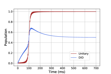
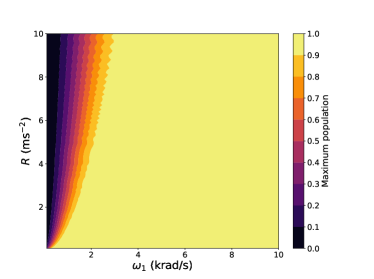
(a) (b)
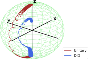
(c) (d)

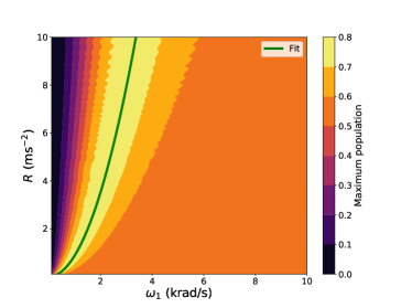
Figure 2: Rectangular pulse. (a) The population transferred from the ground state to the excited state is plotted with respect to time for the unitary case, denoted by the brown curve (color online; the upper curve) and the DID case, denoted by the blue curve (color online; the lower curve). Parameter values used: $\delta\omega=10$ k rad/s, $T=200$ ms, $\omega_{1}=1.0$ k rad/s, $R=2\delta\omega/T=0.1$ ms^-2, $\tau_{c}=10^{-2}$ ms. (b) The components of the magnetization vector ($M_{x}$, $M_{y}$, $M_{z}$) are plotted over the unit sphere for the unitary case, denoted by the brown curve (color online; the outer curve) and the DID case, denoted by the blue curve (color online; the inner curve). Parameter values used: $\delta\omega=50$ k rad/s, $\omega_{1}=3.5$ k rad/s, $R=2\delta\omega/T=1.0$ ms^-2, $\tau_{c}=10^{-3}$ ms. The filled contours represent the maximum population transferred to the excited state from the ground state as a function of $\omega_{1}$ and $R$ for the (c) unitary and (d) DID cases. Here, the yellow strip indicates the optimal region where one can achieve the highest transfer in the presence of DID in the range of 0.7 to 0.8. The green line denotes the parabolic fit, which matches the numerical data well. Parameter values used: $\delta\omega=50$ k rad/s, $\tau_{c}=10^{-2}$ ms.

In figure 2-(a), we have plotted the population as a function of time. The brown line denotes the unitary case, and the blue line denotes the DID case. From the plot, we infer that the entire population is initially in the ground state. During the sweep, the ground state population starts decreasing. On the other hand, the excited state population grows up, and finally, at the end of the sweep the excited state population reaches $1$. This shows that we have achieved a complete population transfer from the ground state to the excited state. If the adiabaticity condition were not met in choosing the parameter values, the excited state population would have been less than $1$, and we could not have achieved the complete transfer.

The blue line in figure 2-(a) represents the population vs. time plot for the DID case with $\tau_{c}=10^{-2}$ ms. We observe that the population transfer is affected by DID, and the maximum transfer is reduced depending upon the value of $\omega_{1}$ and $\tau_{c}$ chosen. The transfer profile shows a non-monotonic behavior. At first, the excited state population increases with time, then it reaches the maximum, and after that, its value drops with time and eventually approaches the steady-state value, ${\rho_{\rm\scriptscriptstyle S}}_{,11}={\rho_{\rm\scriptscriptstyle S}}_{,22}=0.5$, as DID causes the saturation of the spin-$1/2$ system. So, the population transfer shows an optimal behavior in the presence of DID.

We can describe the dynamics using the nutating magnetization. In the rotating frame of the drive, there are effectively two fields: one is the frequency sweep $\Delta\omega(t)$ along $z$-direction, that runs from $-\delta\omega$ to $\delta\omega$ and the other is $\omega_{1}$ along $x$-direction. So, there will be an effective field $\omega_{\rm eff}=\sqrt{\Delta\omega^{2}(t)+\omega_{1}^{2}}$, about which the magnetization nutates. The magnetization vector $\mathbf{M}$ follows the effective field $\omega_{\rm eff}$ at every instant while nutating about it.

We plot the magnetization vector over the Bloch sphere in figure 2-(b). As we started from the state $|g\rangle$, which is the eigenstate of $\sigma_{z}$ with corresponding eigenvalue $-1$, $M_{z}$ runs from $-1$ to $1$ for the unitary case, as denoted by the brown curve. The final value of $M_{z}$ becomes $1$ because we remain close to the adiabatic limit. If the adiabaticity condition were not satisfied, the final $M_{z}$ would have been less than $1$. We can see that near the resonance point, i.e. when $\Delta\omega(t)=0$, $M_{z}$ becomes $0$ and $M_{x}$ becomes $-1$, as the effective field is directed along $x$-direction. It is evident that $\mathbf{M}$ moves over the surface of the sphere for the unitary case and tries to follow the effective field at every instant. Here, we also plot the magnetization by incorporating the DID terms, denoted by the blue curve. We notice that the final value of $M_{z}$ is less than $1$, and at the resonance point, the value of $M_{x}$ is also less than $-1$. As a result, the magnetization vector follows a trajectory inside the Bloch sphere.

To observe the dependence of the population transfer on the parameters $\omega_{1}$ and $R$, we show a contour plot of the maximum population transferred to the excited state from the ground state. From the plot in figure 2-(c), we can infer that, for a particular $R$ value, if we increase $\omega_{1}$, the maximum population increases and after a threshold value of $\omega_{1}$, it reaches the highest value 1, that means complete population transfer has taken place. On the other hand, if we fix $\omega_{1}$ value and increase the $R$ value, we see that the maximum population suffers. This behavior of population transfer is in exact agreement with Zener’s formula for transition probability given in the equation (5). From the formula, it can be verified that when $\frac{\omega_{1}^{2}}{R}\gg 1$, we get better population transfer, and $\frac{\omega_{1}^{2}}{R}\ll 1$ results in less population transfer.

Then, we study the population behavior when DID is taken into account. In figure 2-(d), we notice an optimal region in the plot as shown by the yellow strip, where we achieve the highest transfer, in the range $0.7$ to $0.8$. If we go beyond this region, the population transfer falls off. The behavior up to the yellow region can be explained by the LZ theory. However, it fails to explain what happens beyond this yellow region. That means the large orange region (that limits the lower range to 0.5), where DID sets in, and why they reappear. This contour plot captures the competition and the crossover between the LZ effect and DID. The line of optimality separates pre- and post-optimal regions. In the pre-optimal region, the LZ effect dominates, and in the post-optimal region, DID dominates. We shall try to understand this kind of optimal behavior by developing a proper mathematical model in the next part of the paper.

We construct a set of $\omega_{1}$ and $R$ for the optimal population transfer. Next, we fit this set of $\omega_{1}$ and $R$ with a simple polynomial function to understand their functional dependence. The minimum power of $\omega_{1}$ that fits the data is $2$. Hence, we obtain $R\propto\omega_{1}^{2}$ for each point in the optimal yellow region of the contour plot 2-(d). The green line denotes this parabolic fit. It gives a good fit with the numerical data. We can explain the fit from the probability formula. When $\frac{\omega_{1}^{2}}{R}\ll 1$, the probability for population transfer (ARP) for the unitary case is given by,

$$P^{\prime}=1-\exp\left(-\frac{\pi\omega_{1}^{2}}{2R}\right)\approx\frac{\pi\omega_{1}^{2}}{2R}.$$ (13)

So, the leading order term in the expression of $P^{\prime}$ would be proportional to $\frac{\omega_{1}^{2}}{R}$. So, our fit function is taken to be $R=k\omega_{1}^{2}$, and we find that the value of the fitting parameter $k$ is given by $k=0.88\pm 0.01$.

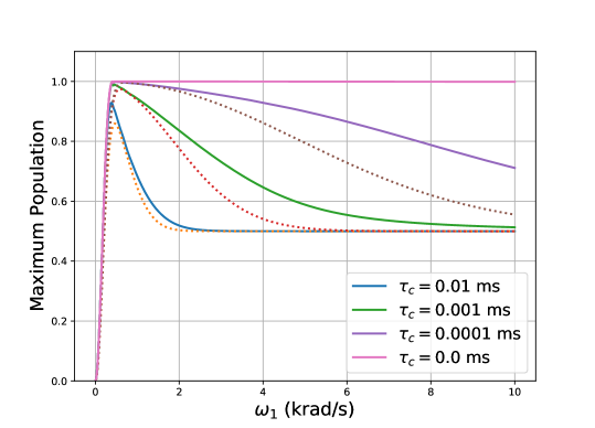
Figure 3: Rectangular pulse. The maximum population transferred to the excited state in the presence of DID is plotted as a function of $\omega_{1}$ for different $\tau_{c}$ values (color online; $\tau_{c}$ values taken in decreasing order, from bottom to top). The dotted lines denote the maximum population curve plotted using our proposed model $p(\omega_{1})$. Parameter values used: $\delta\omega=10$ k rad/s, $R=0.1$ ms^-2.

III.1.1 Existence of optimality: A phenomenological study

From the contour plot 2-(d), we can see that if we move along a constant $R$ value, the maximum population shows a non-monotonic behavior for $\omega_{1}$. At first, it increases with $\omega_{1}$ (which can be explained by LZ formula). However, after crossing the optimal yellow strip, the effect of DID becomes more prominent, and we notice that the population transfer reduces with a subsequent increase in the $\omega_{1}$ value. So, the yellow strip shows the optimal value of $\omega_{1}$, for which we get the best population transfer.

To observe this optimal behavior more concisely, we take a selected slice from the contour plot in the figure 2-(d) for a fixed $R$ value, $R=0.1$ ms^-2 and plotted it with respect to $\omega_{1}$ in figure 3. In figure 3, we can see that the maximum population shows optimality with respect to $\omega_{1}$. When $\omega_{1}$ exceeds a threshold value, the DID effect dominates and dictates the dynamics. Consequently, the population decreases with a further increase in $\omega_{1}$ and finally saturates at the steady-state value $0.5$. In order to check the dependence on $\tau_{c}$, we did the same for various values of $\tau_{c}$. As we increase $\tau_{c}$, the decay becomes more, and the optimal value of $\omega_{1}$ gets shifted towards the origin.

As equation (12) does not have any closed-form analytical solution, we propose a phenomenological model which can explain the behavior shown in figure 2-(d) qualitatively as follows,

$$\mathcal{P}(t)=\frac{1}{2}\left(1-\exp\left(-\frac{\pi\omega_{1}^{2}}{2R}\right)\right)\left[1+\exp(-\omega_{1}^{2}\tau_{c}t)\tanh\left(\frac{R}{\omega_{1}}(t-\delta\omega/R)\right)\right].$$ (14)

We construct the model in the following way:
(i) we begin with the unitary case for which $\tau_{c}=0$, and LZ theory provides the solution for that, i.e. $\left(1-\exp\left(-\frac{\pi\omega_{1}^{2}}{2R}\right)\right)$.
(ii) The temporal behavior, as we observed in the figure 2-(a), is qualitatively captured by a phenomenological factor $\tanh\left(\frac{R}{\omega_{1}}(t-\delta\omega/R)\right)$. Combining (i) and (ii), we get the model for the unitary case as, $\frac{1}{2}\left(1-\exp\left(-\frac{\pi\omega_{1}^{2}}{2R}\right)\right)\left[1+\tanh\left(\frac{R}{\omega_{1}}(t-\delta\omega/R)\right)\right]$.
(iii) To account for the decay due to DID, we phenomenologically introduce a $\tau_{c}$-dependent factor $\exp(-\omega_{1}^{2}\tau_{c}t)$ by multiplying it with the $\tanh\left(\frac{R}{\omega_{1}}(t-\delta\omega/R)\right)$ term and finally arrive at the form given in equation (14).

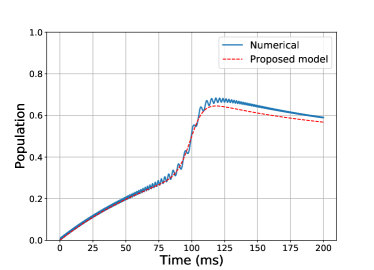
(a) (b)

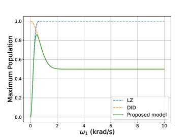
Figure 4: Rectangular pulse. (a) The population transferred from the ground state to the excited state is plotted as a function of time. The solid blue line (color online) represents the numerical data and the dashed red line (color online) represents the population curve plotted using our proposed model $\mathcal{P}(t)$ as a function of time. (b) The maximum population transferred to the excited state for the DID case is plotted using our proposed model $p(\omega_{1})$ as represented by the solid green line. The dashed blue line (color online; the rising curve) represents the transfer described by the conventional LZ formula, and the dashed orange line (color online; the falling curve) represents the decay in the transfer due to DID. There will be a competition between these two effects, leading to an optimal population transfer for a certain value of $\omega_{1}$. Parameter values used: $\delta\omega=10$ k rad/s, $R=0.1$ ms^-2, $\tau_{c}=10^{-2}$ ms.

This model $\mathcal{P}(t)$ predicts a maximum transfer occurring when,

$$\frac{d}{dt}[\mathcal{P}(t)]=0$$

$$\Rightarrow t_{max}=\frac{1}{R}\left[\delta\omega+\frac{\omega_{1}}{2}\sinh^{-1}\left(\frac{2R}{\omega_{1}^{3}\tau_{c}}\right)\right].$$ (15)

In figure 4-(a), we plot the excited state population as a function of time for the DID case. The solid blue line represents the numerically generated data, and the dashed red line denotes the population curve plotted using our proposed model $\mathcal{P}(t)$. Our model provides a reasonably good match with the data, and the peaks occur nearly around the same time. Therefore, $t_{max}$ in equation (15) provides a fair estimation of the occurrence of the optimal point.

Now, as we have seen in figure 3, the chosen slices from the contour data show an optimal transfer for a certain $\omega_{1}$, we use the above model with $t=t_{max}$ to fit the slice data.

We define the maximum population at $t=t_{max}$ as,

$$p(\omega_{1}) = \mathcal{P}(t_{max})$$ (16)

$$= \frac{1}{2}\left(1-\exp\left(-\frac{\pi\omega_{1}^{2}}{2R}\right)\right)\left[1+\exp(-\omega_{1}^{2}\tau_{c}t_{max})\tanh\left(\frac{R}{\omega_{1}}(t_{max}-\delta\omega/R)\right)\right].$$

The above equation (16) represents our model for the maximum population as a function of $\omega_{1}$. This $p(\omega_{1})$ is plotted as a function of $\omega_{1}$ in figure 4-(b) (shown in green). In this figure, the dashed blue line represents the transfer described by the conventional LZ formula for population inversion (ARP), and the dashed orange line leaves the signature of DID. When we take the product of these two, there will be a competition between these two effects- the former LZ factor will try to make the population transfer happen, whereas the latter part coming from DID, causes the population to decay. As a result, we get a non-monotonic behavior as shown by the solid green curve leading to an optimal population transfer for a certain value of $\omega_{1}$.

In figure 3, we also plotted the optimum population as a function of $\omega_{1}$ using our phenomenological model $p(\omega_{1})$ for each $\tau_{c}$ value, as indicated by the dotted lines. Although it does not give an exact match with the numerical data, our focus is to reach close to the maximum (peak) value or, the optimal region in terms of the contour plots. Therefore, the model delivers a qualitative justification for the overall behavior and successfully explains the existence of the optimal behavior in a simple way.

III.2 Gaussian pulse profile

Now, we shall consider a Gaussian pulse profile for the applied drive. That means the amplitude $\omega_{1}$ is no more time-independent; it changes with time in the following manner,

$$\omega_{1}^{gauss}(t)=\omega_{1}^{g}\exp\left(-\frac{(t-T/2)^{2}}{\beta}\right)$$ (17)

where $\beta$ is a measure of the width of the Gaussian and is related to the full-width at half maximum (FWHM) of the Gaussian $\sigma$ as, $\beta=\frac{\sigma^{2}}{4\ln 2}$.

At $t=T/2$, $\omega_{1}^{gauss}(t)=\omega_{1}^{g}$, which is the maximum value that the pulse profile can take. At $t=0$ and $t=T$, $\omega_{1}^{gauss}(t)=\omega_{1}^{g}\exp\left(-\frac{(T/2)^{2}}{\beta}\right)$. Let us suppose we want to cut off the Gaussian at a fraction $f$ of the maximum. That means, At $t=0$ and $t=T$, $\omega_{1}^{gauss}(t)=\omega_{1}^{g}f$. By satisfying the above-mentioned criterion, we find that, $\beta=\frac{(T/2)^{2}}{\ln(\frac{1}{f})}$. For our simulations, we have set $f=0.1$ to truncate the Gaussian profile at $0.1$ of the maximum.

To compare the system dynamics under a rectangular and a Gaussian pulse profile, we ensure that an equal amount of energy has been supplied to the system for both these pulse profiles. We equate the pulse areas of these two profiles and obtain,

$$\omega_{1}^{g}=\frac{\omega_{1}T}{\sqrt{\pi\beta}\>{\rm erf}\left(\frac{T}{2\sqrt{\beta}}\right)}.$$ (18)

The equation (18) provides the relation between $\omega_{1}^{g}$ and $\omega_{1}$ such that the equal area condition is satisfied. This relation will be used for the subsequent simulations with a Gaussian pulse. In equation (17), we have chosen the Gaussian profile in such a way that its duration remains $T$, which is the same as that of the rectangular pulse profile. So, on physical grounds, we can argue that to keep the area of both these profiles constant within the same duration, the peak value (maximum) of the Gaussian $\omega_{1}^{g}$ has to be much higher than $\omega_{1}$ (the maximum amplitude of the rectangular pulse). This can be verified from equation (18) as well by putting some numerical value for $T$. For $T=200$ ms, we have checked that, $\omega_{1}^{g}=1.7686\;\omega_{1}$, that means $\omega_{1}^{g}>\omega_{1}$.

In figure 5-(a), we plot the population with respect to time. We have kept the parameter values the same as that taken for the rectangular profile: $\delta\omega$ = 10 k rad/s, $\omega_{1}$ = 1 k rad/s, $T$ = 200 ms, $R=2\delta\omega/T$ = 0.1 ms^-2. We can see that a Gaussian pulse results in a much smoother population behavior than a rectangular pulse with an equal area. Also, we note that for the same parameter values of $\omega_{1}$ and $R$, we achieve better steady-state population transfer for the DID case, using a Gaussian pulse.

In the magnetization plot over the Bloch sphere for DID case, shown in figure 5-(b), we see that the magnetization vector follows a trajectory inside the Bloch sphere. In contrast to the same plot done for a rectangular pulse profile, here we note that initially $M_{z}$ decays very slowly. This happens because near $t=0$, $\omega_{1}^{gauss}(t)=\omega_{1}^{g}f=0.1\;\omega_{1}^{g}=0.17686\;\omega_{1}$, for our chosen parameter values; i.e., $\omega_{1}^{gauss}(t)<\omega_{1}$. As a result, it does not exhibit any significant decay along the $z$-direction, and the overall nature of the magnetization curve is very smooth.

In figure 5-(d), we have done the contour plot of the maximum population transferred to the excited state from the ground state when DID is taken into account. Here also, we obtain a similar optimal behavior of population transfer. However, the strips become narrower in this case and the highest transfer increases to 0.9. That means we achieve a more efficient transfer. In addition to that, we notice that the optimal yellow region occurs for a lower range of $\omega_{1}$ values, implying that we can achieve more transfer by applying a drive of relatively lower amplitude. Therefore, frequency sweep using a Gaussian pulse results in better and more efficient population transfer. Here, we fit the contour data in the optimal yellow region with a parabolic fit, as shown by the green line. So, our fit function is taken to be $R=k\omega_{1}^{2}$, and the fitting parameter $k$ turns out to be $k=2.17\pm 0.04$, for this case.

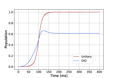
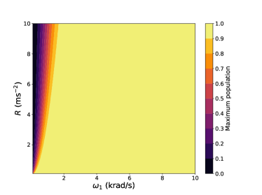
(a) (b)
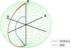
(c) (d)

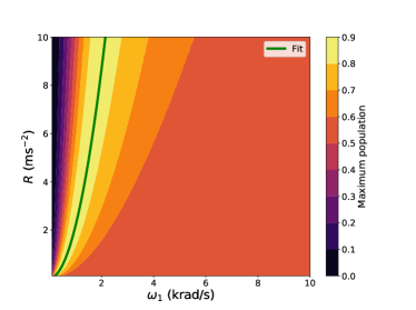
Figure 5: Gaussian pulse. (a) The population transferred from the ground state to the excited state is plotted with respect to time for the unitary case, denoted by the brown curve (color online; the upper curve) and the DID case, denoted by the blue curve (color online; the lower curve). Parameter values used: $\delta\omega=10$ k rad/s, $T=200$ ms, $\omega_{1}=1.0$ k rad/s, $R=2\delta\omega/T=0.1$ ms^-2, $\tau_{c}=10^{-2}$ ms. (b) The components of the magnetization vector ($M_{x}$, $M_{y}$, $M_{z}$) are plotted over the unit sphere for the unitary case, denoted by the brown curve (color online; the outer curve) and the DID case, denoted by the blue curve (color online; the inner curve). Parameter values used: $\delta\omega=50$ k rad/s, $\omega_{1}=3.5$ k rad/s, $R=2\delta\omega/T=1.0$ ms^-2, $\tau_{c}=10^{-3}$ ms. The filled contours represent the maximum population transferred to the excited state from the ground state as a function of $\omega_{1}$ and $R$ for the (c) unitary and (d) DID cases. Here, the yellow strip indicates the optimal region where one can achieve the highest transfer in the presence of DID in the range of 0.7 to 0.8. The green line denotes the parabolic fit, which matches the numerical data well. Parameter values used: $\delta\omega=50$ k rad/s, $\tau_{c}=10^{-2}$ ms.

IV Discussions

We have shown that DID affects the ARP; thus, the population transfer suffers. DID prevents the complete transfer achieved under unitary dynamics. When DID is included in the dynamics, we find an optimal value of the population transfer, which is less than 1 (for the excited state). Furthermore, this implies that since the population transfer gets reduced due to DID, the system is likely to make a transition from $E_{+}(t)$ to $E_{-}(t)$ or vice-versa, which is nothing but an LZ transition.

This work shows that optimality exists in transferring population in a TLS using a frequency sweep model. In the presence of DID, population transfer shows a non-monotonic behavior with respect to time as well as $\omega_{1}$. In the time-series plot, we have observed that the population hits the maximum at a certain time, which we denote as $t_{max}$, and gradually, it decays down to the steady-state value (which is 0.5 for rectangular pulse profile). Therefore, we need to turn off the drive at $t=t_{max}$ to achieve the best transfer. In the contour plot of the maximum population in $R$ vs. $\omega_{1}$ plane, the yellow strip signifies the optimal region. We need to choose the parameters $R$ and $\omega_{1}$ suitably so that we can arrive at this region to get the most efficient transfer.

Here, we choose the relaxation times $T_{1}$ and $T_{2}$ to be large, such that the decoherence due to system-environment coupling becomes negligibly small. So, the nonunitary behavior originates principally due to DID. But, in situations where the system-environment coupling dominates over DID, we must include the contribution from the relaxation processes. In such cases, we would see that population transfer is affected due to system-environment coupling. With time, the population would finally saturate at the equilibrium values, ${\rho_{\rm\scriptscriptstyle S}}_{,11}=\frac{1+M_{0}}{2}$ and ${\rho_{\rm\scriptscriptstyle S}}_{,22}=\frac{1-M_{0}}{2}$.

We propose a qualitative model to explain the optimal behavior that we observe in ARP for a rectangular pulse. The factor coming from the conventional LZ formula is responsible for the initial growth in population transfer. But as $\omega_{1}$ becomes sufficiently large to have an impact of DID on the dynamics, the transfer starts to decay with $\omega_{1}$. Therefore, there exists an optimum value of $\omega_{1}$ for which the transfer hits the maximum.

We have extended our analysis to shaped pulses. We have found that using a Gaussian pulse over a rectangular pulse is a better and more efficient option to achieve population transfer by supplying an equal amount of energy. When we look at the steady-state behavior of population transfer as shown in figure 2-(a) and figure 5-(a), we can conclude that for a Gaussian pulse, the transfer finally saturates at a higher value. This behavior can be explained in the following way: At $t=T/2$, $\omega_{1}^{gauss}(t)$ attains the maximum value $\omega_{1}^{g}$, and when $t>T/2$ (or, $t<T/2$), the value of $\omega_{1}^{gauss}(t)$ eventually decreases with time. When $t=T$, $\omega_{1}^{gauss}(t)=\omega_{1}^{g}f=0.1\;\omega_{1}^{g}$, for $f=0.1$, which is definitely less than $\omega_{1}$ (the amplitude of the rectangular pulse throughout the duration $T$). Therefore towards the end of the Gaussian pulse, the DID is small and is insufficient to cause a saturation at $0.5$. So, the final steady state value of the excited state population remains above $0.5$. It is noteworthy that had we chosen a higher cut-off fraction for the Gaussian profile instead of $f=0.1$, the effect of DID would have been more prominent, and the steady-state behavior would look very similar to the rectangular pulse.

From the contour plots of maximum population transfer for a Gaussian pulse, we can see that in figure 5-(d), the upper limit of the color bar has increased to 0.9, whereas for a rectangular pulse, it was 0.8. Moreover, the filled contours (strips) have become narrower, smoother, and shifted towards the origin. This implies that applying a drive with a lower strength (low $\omega_{1}$) can achieve better transfer using a Gaussian pulse. Therefore, a Gaussian pulse provides higher efficiency in population transfer using ARP than a rectangular pulse.

V Conclusions

We have implemented population transfer in a TLS by ARP using a linear chirped while including the dissipative effects coming from the applied drive in our study. Most interestingly, we have found that, even within the adiabatic limit, the population inversion suffers from the detrimental effects of DID. Further, we have shown that the population transfer exhibits an optimal behavior as a result of the competing processes like the conventional LZ effect and DID. The values of $\omega_{1}$ and $\tau_{c}$ decide the maximum value the transferred population can acquire. Not only the temporal behavior, the population transfer behaves non-monotonically as a function of the sweep rate $R$ and the drive amplitude $\omega_{1}$ also. We show that a truncated chirped pulse that stops at the point where optimality is achieved yields the best possible transfer. We proposed a phenomenological model to qualitatively explain the transfer behavior to estimate the optimal point. We have analyzed both rectangular and Gaussian pulse profiles and have shown that the Gaussian profile gives a more efficient result than the rectangular profile. We contemplate that our results would be beneficial for the practitioners of ARP, and they would be able to achieve the optimal population transfer in realistic experimental set-ups.

References

- Zener (1932) C. Zener, in Proc. R. Soc. London A (1932) pp. 696–702.
- Landau (1932a) L. D. Landau, Phys. Z. Sowjetunion 1, 88 (1932a).
- Landau (1932b) L. D. Landau, Phys. Z. Sowjetunion 2, 46 (1932b).
- Matsuzawa (1968) M. Matsuzawa, Journal of the Physical Society of Japan 25, 1153 (1968), publisher: The Physical Society of Japan.
- Baede et al. (1969) A. P. M. Baede, A. M. C. Moutinho, A. E. de Vries, and J. Los, Chemical Physics Letters 3, 530 (1969).
- Olson (1970) R. E. Olson, Physical Review A 2, 121 (1970).
- Zwally and Cable (1971) H. J. Zwally and P. G. Cable, Physical Review A 4, 2301 (1971).
- Abragam (1961) A. Abragam, The principles of nuclear magnetism, 32 (Oxford university press, 1961).
- Bloch (1946) F. Bloch, Phys. Rev. 70, 460 (1946).
- Drain (1949) L. E. Drain, Proc. Phys. Soc. A 62, 301 (1949).
- Chiarotti et al. (1954) G. Chiarotti, G. Cristiani, L. Giulotto, and G. Lanzi, Nuovo Cim 12, 519 (1954).
- Redfield (1956) A. G. Redfield, Phys. Rev. 101, 67 (1956).
- Abragam and Proctor (1958) A. Abragam and W. G. Proctor, Phys. Rev. 109, 1441 (1958).
- Slichter and Holton (1961) C. P. Slichter and W. C. Holton, Phys. Rev. 122, 1701 (1961).
- Janzen et al. (1968) W. R. Janzen, T. J. R. Cyr, and B. A. Dunell, The Journal of Chemical Physics 48, 1246 (1968).
- Herbers et al. (2022) S. Herbers, Y. M. Caris, S. E. J. Kuijpers, J.-U. Grabow, and S. Y. T. van de Meerakker, Molecular Physics 0, e2129105 (2022).
- Kaprálová-Žďánská et al. (2022) P. R. Kaprálová-Žďánská, M. Šindelka, and N. Moiseyev, J. Phys. A: Math. Theor. 55, 284001 (2022).
- Chen et al. (2021) J. Chen, L. Deng, Y. Niu, and S. Gong, Phys. Rev. A 103, 053705 (2021).
- Feilhauer et al. (2020) J. Feilhauer, A. Schumer, J. Doppler, A. A. Mailybaev, J. Böhm, U. Kuhl, N. Moiseyev, and S. Rotter, Phys. Rev. A 102, 040201(R) (2020).
- Mukherjee et al. (2020) A. Mukherjee, A. Widhalm, D. Siebert, S. Krehs, N. Sharma, A. Thiede, D. Reuter, J. Förstner, and A. Zrenner, Appl. Phys. Lett. 116, 251103 (2020).
- Melinger et al. (1992) J. S. Melinger, S. R. Gandhi, A. Hariharan, J. X. Tull, and W. S. Warren, Phys. Rev. Lett. 68, 2000 (1992).
- Melinger et al. (1994) J. S. Melinger, S. R. Gandhi, A. Hariharan, D. Goswami, and W. S. Warren, The Journal of Chemical Physics 101, 6439 (1994).
- Malinovsky and Krause (2001) V. Malinovsky and J. Krause, The European Physical Journal D 14, 147 (2001).
- Maeda et al. (2006) H. Maeda, J. H. Gurian, D. V. L. Norum, and T. F. Gallagher, Phys. Rev. Lett. 96, 073002 (2006).
- Ao and Rammer (1989) P. Ao and J. Rammer, Phys. Rev. Lett. 62, 3004 (1989).
- Ao and Rammer (1991) P. Ao and J. Rammer, Phys. Rev. B 43, 5397 (1991).
- Ashhab (2016) S. Ashhab, Phys. Rev. A 94, 042109 (2016).
- Nalbach and Thorwart (2009) P. Nalbach and M. Thorwart, Phys. Rev. Lett. 103, 220401 (2009).
- Wubs et al. (2006) M. Wubs, K. Saito, S. Kohler, P. Hänggi, and Y. Kayanuma, Phys. Rev. Lett. 97, 200404 (2006).
- Sun et al. (2016) Z. Sun, L. Zhou, G. Xiao, D. Poletti, and J. Gong, Phys. Rev. A 93, 012121 (2016).
- Whitney et al. (2011) R. S. Whitney, M. Clusel, and T. Ziman, Phys. Rev. Lett. 107, 210402 (2011).
- Chakrabarti and Bhattacharyya (2018a) A. Chakrabarti and R. Bhattacharyya, Phys. Rev. A 97, 063837 (2018a).
- Rubbmark et al. (1981) J. R. Rubbmark, M. M. Kash, M. G. Littman, and D. Kleppner, Phys. Rev. A 23, 3107 (1981).
- Chakrabarti and Bhattacharyya (2018b) A. Chakrabarti and R. Bhattacharyya, EPL (Europhysics Letters) 121, 57002 (2018b).
- Chanda and Bhattacharyya (2020) N. Chanda and R. Bhattacharyya, Phys. Rev. A 101, 042326 (2020).
- Chanda and Bhattacharyya (2021) N. Chanda and R. Bhattacharyya, Phys. Rev. A 104, 022436 (2021).
- Chatterjee and Bhattacharyya (2020) A. Chatterjee and R. Bhattacharyya, Phys. Rev. A 102, 043111 (2020).
- Saha and Bhattacharyya (2022) S. Saha and R. Bhattacharyya, J. Phys. B: At. Mol. Opt. Phys. 55, 235501 (2022).