Canonical momentum based numerical schemes for hybrid plasma models with kinetic ions and massless electrons

Abstract

We study the canonical momentum based discretizations of a hybrid model with kinetic ions and mass-less electrons. Two equivalent formulations of the hybrid model are presented, in which the vector potentials are in different gauges and the distribution functions depend on canonical momentum (not velocity). Particle-in-cell methods are used for the distribution functions, and the vector potentials are discretized by the finite element methods in the framework of finite element exterior calculus. Splitting methods are used for the time discretizations. It is illustrated that the second formulation is numerically superior and the schemes constructed based on the anti-symmetric bracket proposed have better conservation properties, although the filters can be used to improve the schemes of the first formulation.

1 Introduction

There are a lot of models proposed to describe complex physical processes in plasmas, which usually include different kinds of species and are inherently multi-scale. Among them, hybrid models combine the advantages of kinetic and fluid models, in which some components of plasmas, such as high energy particles, are treated kinetically, while the remainder is described using fluid type equations. Compared to kinetic equations, hybrid models are more computationally efficient because of the fluid equations adopted and small scales ignored. Also they are more accurate than pure fluid type models, as kinetic effects of some components are included. There are many kinds of hybrid kinetic-fluid models for plasmas in literature in different contexts [27, 28, 29].

In magnetized kinetic plasma simulations, the distribution function of each particle species depends on velocity ${\mathbf{v}}$ or canonical momentum ${\mathbf{p}}$, which have the relation $m_{i}{\mathbf{v}}={\mathbf{p}}-q_{i}{\mathbf{A}}$, where ${\mathbf{A}}$ denotes the vector potential and $m_{i},q_{i}$ are the mass and charge of each particle species. Also the magnetic field can be represented by the magnetic field ${\mathbf{B}}$ or the vector potential ${\mathbf{A}}$ via the formula ${\mathbf{B}}=\nabla\times{\mathbf{A}}$. So for the magnetized kinetic/hybrid models, there are three kinds of formulations with different choices of unknowns, 1). $xvB$ formulation, which includes the distribution functions depending on velocity and the magnetic field as unknowns; 2). $xvA$ formulation, which includes the distribution functions depending on velocity and the vector potential as unknowns; 3). $xpA$ formulation, which includes the distribution functions depending on the canonical momentum and the vector potential as unknowns. The Poisson brackets of $xvB$ and $xvA$ formulations, if there are, can usually be derived from the counterparts of $xpA$ formulations by using the chain rules of the functional derivatives, and the former usually have more terms and are more complicated than the latter, which reflects the differences of coupling complexity.

There have been some numerical simulation works based on the $xpA$ formulations in different contexts. For the fully kinetic equations, in [2] canonical symplectic methods are proposed based on the discretization of the Poisson bracket of the Vlasov–Maxwell equations. For the gyro-kinetic simulations [41] with strong magnetic fields, parallel canonical momentum is used as an independent variables of the distribution functions to avoid the term of the time derivative of $A_{\parallel}$ in the Vlasov equation. Some recent developments include [42, 43]. In the context of the hybrid plasma simulations, the $xvB$ and $xvA$ formulations are adopted numerically in most research works [36, 29, 21, 22, 28, 38, 39, 40], and the $xpA$ formulation has been used in [36] and the references therein, in which it is called the ’Hamiltonian method’.

In this work, we consider the numerical discretizations for the $xpA$ formulations of a hybrid model, in which all ions are treated kinetically, electrons are mass-less, and the electron pressure is determined by the electron density via the equation of state. This model has many applications in laser plasmas and astrophysics [26, 45, 46, 47], and is obtained by taking quasi-neutral limit and mass-less electron limit for the more fundamental models. For simplicity we consider the one ion species case and assume each ion has a unit charge. The commonly used $xvB$ formulation of this model after the dimensionless procedures in [20] is

$$\frac{\partial f}{\partial t}=-{\mathbf{v}}\cdot\nabla f-({\mathbf{E}}+{\mathbf{v}}\times{\mathbf{B}})\cdot\nabla_{v}f,$$ (1)

$$\frac{\partial{\mathbf{B}}}{\partial t}=-\nabla\times{\mathbf{E}},$$

where

$${\mathbf{E}}=-\frac{\nabla p_{e}}{n}-{\mathbf{u}}\times{\mathbf{B}}+\frac{\mathbf{J}}{n}\times{\mathbf{B}}\ (\text{Ohm's law})$$ (2)

with

$${\mathbf{J}}=\nabla\times{\mathbf{B}},\quad n=\int f\mathrm{d}{\mathbf{v}},\quad n{\mathbf{u}}=\int f{\mathbf{v}}\mathrm{d}{\mathbf{v}}.$$

Here $f$ is the distribution function of ions depending on time $t$, space ${\mathbf{x}}$, and velocity ${\mathbf{v}}$. ${\mathbf{E}}$ and ${\mathbf{B}}$ are electric and magnetic fields, respectively. The $n$ is the density of electrons, which equals to the density of ions $\int f\mathrm{d}{\mathbf{v}}$ because of the quasi-neutrality condition. In the above Ohm’s law, $p_{e}$ is the electron pressure, which is commonly taken to be $nT$ in the isothermal electron case with constant $T$ (the normalized temperature of electrons) or $Cn^{\gamma}$ with $\gamma\neq 1$ in the adiabatic electron case with constant $C$. In more general cases, a time evolution equation of $p_{e}$ should be included in the hybrid model (1) as [21]. Existing numerical methods for this formulation include current advance method [17], based on which, there is a particle-in-cell code CAMELIA [18] and an Eulerian code [19]; Pegasus [24], in which a constrained transport method is used to guarantee the divergence free property of magnetic field; mass and energy conserving particle-in-cell schemes on curvilinear meshes [22], which also conserve momentum provided the magnetic field is divergence free. Also structure-preserving particle-in-cell schemes are constructed in [20] based on an anti-symmetric bracket and splitting methods, which conserve many properties at the same time, such as energy, quasi-neutrality condition, and divergence free property of magnetic field. For more reviews about hybrid simulations, we refer the readers to the references [37, 29]. The difficulty in hybrid-kinetic codes for $xvB$ formulation is obtaining an accurate time-advanced electric field, which is necessary to get second-order-accurate pushers of the particles and the updates of the magnetic field. The $xvA$ formulation can be obtained by just replacing ${\mathbf{B}}$ by $\nabla\times{\mathbf{A}}$ (${\mathbf{A}}$ is the vector potential) in the $xvB$ formulation (1). Recently, there are some numerical schemes conserving energy, momentum, and mass proposed in [21] based on the $xvA$ formulation using particle-in-cell methods combined with finite difference methods, in which an equation of electron pressure is used. As the vector potential is used, the divergence free property of the magnetic field obtained is guaranteed naturally.

In this work, the two $xpA$ formulations we investigate numerically are with different gauges of the vector potential. In the first $xpA$ formulation (or formulation I), the Weyl gauge is chosen for the vector potential, while in the second $xpA$ formulation (or formulation II), a different gauge is used due to that the electron pressure term is a gradient term in the isothermal and adiabatic electrons cases. The characteristics of Vlasov equation in $xpA$ formulations constitute canonical Hamiltonian systems, for which symplectic methods [5, 9] and discrete gradient methods [31] can be used to solve. However, in $xvB$ and $xpA$ formulations pushing particle is more complicated due to the complex electric field ${\mathbf{E}}$ depending on all the particles in the Ohm’s law, which is quite common in various hybrid models [3, 16]. In [36] and some references therein, updating particles using the canonical momentum is introduced, but the relation of the electron pressure term with the gauge in the isothermal and adiabatic electron cases is not mentioned. This idea of changing the gauge used can also be applied to the $xvA$ formulation investigated in [21] with the anti-symmetric bracket presented in appendix 6.2 and relativistic hybrid models [34].

Our discretizations follow the recent developments of structure-preserving methods for models in plasma physics with the aim of having better long term numerical behaviours. Fully discrete structure-preserving particle-in-cell methods for the Vlasov–Maxwell equations have been proposed in [4, 2] using the finite difference methods in the framework of discrete exterior calculus [11], and in [13, 1, 35] using the finite element methods in the framework of finite element exterior calculus [10]. In [4, 13, 1, 35] the time discretizations are done using the Hamiltonian splitting methods firstly proposed in [49] with a correction provided in [50, 51]. For electrostatic hybrid plasma simulations, structure preserving algorithms have been constructed in [7].

In this work, for the two $xpA$ formulations, we discretize the vector potentials by finite element methods in the framework of finite element exterior calculus [10], and the distribution functions are approximated as the sums of finite number of weighted particles. Splitting methods [9] are used in time to give two subsystems, for which implicit mid-point rules are used to solve. For the formulation I with the Weyl gauge, a projector is used to deal with the electron pressure term to make it only contribute to the curl free part of the vector potential. Some binomial filters are applied for the electron pressure to reduce the noises from the particle methods ($n$ is obtained by depositions of particles), which improves significantly the schemes. For the formulation II, Poisson splitting [12] is used based on the anti-symmetric bracket proposed, and the schemes constructed have better conservation properties. The implementations are done in the Python package STRUPHY [6].

There are some connections between our recent work [20] and the formulation II. The bracket proposed in [20] could be derived from the bracket of formulation II using the chain rules of the functional derivatives. The methods constructed in this work for the formulation II have the following advantages. 1) Particles are updated by solving simple canonical Hamiltonian systems, which is good for structure-preserving property and good long time behaviors; 2) It is easier to do the implementations than [20], as only two subsystems are obtained after Poisson splitting [12] in time, particles and fields are decoupled. 3) The algorithms obtained are more efficient, as some heavy iterations about particles and projectors for current terms in [20] are avoided; 4) The property of divergence-free of the magnetic fields is guaranteed naturally as the vector potential is used and discretized in a $H(\text{curl})$ type finite element space.

This paper is organized as follows. Two canonical momentum based formulations of the hybrid model are presented in section 2, for which phase-space and time discretizations are done in section 3. In section 4, four numerical experiments: finite grid instability, R-wave, Bernstein waves, and ion cyclotron instability are conducted to validate the codes, and comparisons are made. In section 5, we conclude the paper with a summary and an outlook to future works.

2 Canonical momentum based formulations

In this section, we present two equivalent formulations of the hybrid model, in which the distribution functions depend on the canonical momentum, and the vector potentials are used. For simplicity we focus on the isothermal electron case, i.e., $p_{e}=nT$, similar results can be obtained for the adiabatic electron case. As we shall see, the main differences between these two formulations are where the term $T\frac{\nabla n}{n}$ appears and how it influences the update of the particles. The first $xpA$ formulation is obtained as follows by choosing the vector potential in Weyl gauge, this gauge is used in many plasma simulations, such as [2, 21].
Formulation I: by change of unknowns as ${\mathbf{B}}=\nabla\times{\mathbf{A}}$ (${\mathbf{A}}$ is the Weyl gauge) and $f(t,{\mathbf{x}},{\mathbf{v}})=f(t,{\mathbf{x}},{\mathbf{p}}-{\mathbf{A}})=:f_{m}(t,{\mathbf{x}},{\mathbf{p}})$, we have the equations about $f_{m}$ (still denoted by $f$ for convenience) and ${\mathbf{A}}$ from equations (1),

$$\frac{\partial f}{\partial t}=-({\mathbf{p}}-{\mathbf{A}})\cdot\frac{\partial f}{\partial{\mathbf{x}}}+\left[\left(\frac{\partial{\mathbf{A}}}{\partial\mathbf{x}}\right)^{\top}({\mathbf{A}}-{\mathbf{p}})\right]\cdot\frac{\partial f}{\partial{\mathbf{p}}},$$ (3)

$$\frac{\partial{\mathbf{A}}}{\partial t}=T\frac{\nabla n}{n}-\frac{\nabla\times\nabla\times{\mathbf{A}}}{n}\times{\nabla\times{\mathbf{A}}}-\frac{\int({\mathbf{A}}-{\mathbf{p}})f\mathrm{d}{\mathbf{p}}}{n}\times{\nabla\times{\mathbf{A}}},\quad n=\int f\mathrm{d}{\mathbf{p}}.$$

We can see that the term $T\frac{\nabla n}{n}$ influences the update of the particles through the vector potential. The total energy of the $xpA$ formulation (3) is

$$\mathcal{H}=\frac{1}{2}\int f|{\mathbf{p}}-{\mathbf{A}}|^{2}\mathrm{d}{\mathbf{x}}\mathrm{d}{\mathbf{p}}+T\int n\ln n\mathrm{d}{\mathbf{x}}+\frac{1}{2}\int|\nabla\times{\mathbf{A}}|^{2}\mathrm{d}{\mathbf{x}}.$$ (4)

Here the density of electrons $n$ is not regarded as an independent unknown, the reason is that when $n$ is regarded as an independent unknown, conserving the quasi-neutrality relation $n=\int f\mathrm{d}{\mathbf{v}}$ and the positivity of $n$ is not easy to achieve numerically, although the system (3) with the time evolution equation of $n$, i.e., $\partial_{t}n+\nabla\cdot(n{\mathbf{u}})=0$, is a Hamiltonian system with a Poisson bracket proposed in [3]. As $T\frac{\nabla n}{n}$ is the gradient of $T\ln n$, it has no contribution for the magnetic field $\nabla\times{\mathbf{A}}$. Also numerically, $n$ is obtained from particles by depositions, then $n$ and $T\frac{\nabla n}{n}$ have a lot of noises and would make the update of ${\mathbf{A}}$ not accurate. These inspire us to change the gauge used, and choose the gauge of ${\mathbf{A}}$ satisfying

$${\mathbf{E}}=-T\frac{\nabla n}{n}-\frac{\partial{\mathbf{A}}}{\partial t}.$$

Then we get the following equivalent formulation.
Formulation II:

$$\frac{\partial f}{\partial t}=-({\mathbf{p}}-{\mathbf{A}})\cdot\frac{\partial f}{\partial{\mathbf{x}}}+\left[T\frac{\nabla n}{n}+\left(\frac{\partial{\mathbf{A}}}{\partial\mathbf{x}}\right)^{\top}({\mathbf{A}}-{\mathbf{p}})\right]\cdot\frac{\partial f}{\partial{\mathbf{p}}},$$ (5)

$$\frac{\partial{\mathbf{A}}}{\partial t}=-\frac{\nabla\times\nabla\times{\mathbf{A}}}{n}\times{\nabla\times{\mathbf{A}}}-\frac{\int({\mathbf{A}}-{\mathbf{p}})f\mathrm{d}{\mathbf{p}}}{n}\times{\nabla\times{\mathbf{A}}},\quad n=\int f\mathrm{d}{\mathbf{p}},$$

in which the term $T\frac{\nabla n}{n}$ appears in the Vlasov equation and has a direct interaction with particles. The total energy of the second $xpA$ formulation (5) is

$$\mathcal{H}=\frac{1}{2}\int f|{\mathbf{p}}-{\mathbf{A}}|^{2}\mathrm{d}{\mathbf{x}}\mathrm{d}{\mathbf{p}}+T\int n\ln n\mathrm{d}{\mathbf{x}}+\frac{1}{2}\int|\nabla\times{\mathbf{A}}|^{2}\mathrm{d}{\mathbf{x}}.$$ (6)

The formulation (5) can be derived from the following anti-symmetric bracket (7) with energy (6),

$$\{\mathcal{F},\mathcal{G}\}(f,{\mathbf{A}}) =\int f\left[\frac{\delta\mathcal{F}}{\delta f},\frac{\delta\mathcal{G}}{\delta f}\right]_{xp}\mathrm{d}{\mathbf{x}}\mathrm{d}{\mathbf{p}}-\int\frac{1}{n}\nabla\times\mathbf{A}\cdot\left(\frac{\delta\mathcal{F}}{\delta{\mathbf{A}}}\times\frac{\delta\mathcal{G}}{\delta{\mathbf{A}}}\right)\mathrm{d}{\mathbf{x}},$$ (7)

where the two terms are responsible for the derivations of the two equations in (5), respectively. The anti-symmetric bracket (7) is the foundation for us to use the Poisson splitting [12] in time for this formulation (5) in the next section, which gives two sub-systems. As we shall see, the subsystem of the Vlasov equation is discretized as a canonical Hamiltonian system, for which symplectic methods [9] or discrete gradient methods [31, 15] can be used for the time discretization. The term $T\frac{\nabla n}{n}$ interacts with the particles directly, and the schemes constructed are more accurate, which are presented and explained qualitatively and quantitively in the remaining parts of this work.

Remark 1.

When there is a given background magnetic field ${\mathbf{B}}_{0}$, complete equations of the above two formulations are presented in Appendix 6.1.

3 Numerical discretization

In this section, we use the finite element method in the framework of finite element exterior calculus to discretize the vector potential, and particle-in-cell method to discretize the distribution function. Splitting methods are used in time for two formulations (3) and (5). Also binomial filters are introduced, which would be used in the section 4 to reduce the noises of the particle methods of the formulation I (3). Time step size is $\Delta t$, $a^{n}$ means the value of $a$ at $n-$th time step, and $a^{n+\frac{1}{2}}$ represents $\frac{a^{n}+a^{n+1}}{2}$.

Commuting diagram with B-splines We perform the spatial discretizations in the framework of Finite Element Exterior Calculus (FEEC). Finite element (FE) spaces and corresponding projectors are chosen such that the following diagram commutes,

(8)

where $V_{0},V_{1},V_{2}$ and $V_{3}$ are finite element spaces in which fields (proxies of $p$-forms, $p\leq 3$) are discretized in. The projectors $\Pi_{n}$ are based on inter-/histopolation at/between Greville points of the B-splines which span the FE spaces. For details we refer to [6] which uses exactly the same basis functions and projectors. The FE spaces are written as

$$V_{0}:=\text{span}\{\Lambda^{0}_{i}|0\leq i<N_{0}\}, \ni{a}^{0}_{h}(t,{\mathbf{x}})=\sum_{i=0}^{N_{0}-1}a_{i}(t)\Lambda^{0}_{i}({\mathbf{x}})$$

$$V_{1}:=\text{span}\left\{\left(\begin{matrix}\Lambda^{1}_{1,i}\\ 0\\ 0\end{matrix}\right),\left(\begin{matrix}0\\ \Lambda^{1}_{2,i}\\ 0\end{matrix}\right),\left(\begin{matrix}0\\ 0\\ \Lambda^{1}_{3,i}\end{matrix}\right)\Bigg{|}\begin{matrix}0\leq i<N^{1}_{1}\\ 0\leq i<N^{1}_{2}\\ 0\leq i<N^{1}_{3}\end{matrix}\right\} \ni{\mathbf{a}}^{1}_{h}(t,{\mathbf{x}})=\sum_{\mu=1}^{3}\sum_{i=1}^{N_{\mu}^{1}-1}a_{\mu,i}(t)\Lambda^{1}_{\mu,i}({\mathbf{x}}){\mathbf{e}}_{\mu},$$

$$V_{2}:=\text{span}\left\{\left(\begin{matrix}\Lambda^{2}_{1,i}\\ 0\\ 0\end{matrix}\right),\left(\begin{matrix}0\\ \Lambda^{2}_{2,i}\\ 0\end{matrix}\right),\left(\begin{matrix}0\\ 0\\ \Lambda^{2}_{3,i}\end{matrix}\right)\Bigg{|}\begin{matrix}0\leq i<N^{2}_{1}\\ 0\leq i<N^{2}_{2}\\ 0\leq i<N^{2}_{3}\end{matrix}\right\} \ni{\mathbf{a}}^{2}_{h}(t,{\mathbf{x}})=\sum_{\mu=1}^{3}\sum_{i=1}^{N_{\mu}^{1}-1}a_{\mu,i}(t)\Lambda^{2}_{\mu,i}({\mathbf{x}}){\mathbf{e}}_{\mu},$$

$$V_{3}:=\text{span}\{\Lambda^{3}_{i}|0\leq i<N_{3}\}, \ni{a}^{3}_{h}(t,{\mathbf{x}})=\sum_{i=0}^{N_{3}-1}a_{i}(t)\Lambda^{3}_{i}({\mathbf{x}})\,.$$

Here, the functions $\Lambda_{i}^{n}:\Omega\to\mathbb{R}$ are tensor products of uni-variate B-splines of different degree, as described in [6, 1], and ${\mathbf{e}}_{1}=(1,0,0)^{\top}$, ${\mathbf{e}}_{2}=(0,1,0)^{\top}$, ${\mathbf{e}}_{3}=(0,0,1)^{\top}$. The dimensions are

$$\textnormal{dim}V_{0}=N_{0}\,,\quad\textnormal{dim}V_{1}=N_{1}=\sum_{d=1}^{3}N^{1}_{d}\,,\quad\textnormal{dim}V_{2}=N_{2}=\sum_{d=1}^{3}N^{2}_{d}\,,\quad\textnormal{dim}V_{3}=N_{3}\,.$$ (9)

To simplify the notation, we stack the FE coefficients $a_{i}$ and basis functions in column vectors, e.g. ${\mathbf{a}}:=(a_{i})_{0\leq i<N_{0}}\in\mathbb{R}^{N_{0}}$, and ${{\mathbf{\Lambda}}^{0}}:=(\Lambda^{0}_{i})_{0\leq i<N_{0}}\in\mathbb{R}^{N_{0}}$. Spline functions can then be compactly written as

$${a}_{h}^{0}={\mathbf{a}}^{\top}{\mathbf{\Lambda}}^{0},$$

$$({\mathbf{a}}_{h}^{1})^{\top}=(\underbrace{a_{1,0},\cdots,a_{1,N^{1}_{1}-1}}_{=:{\mathbf{a}}_{1}^{\top}},\underbrace{a_{2,0},\cdots,a_{2,N^{1}_{2}-1}}_{=:{\mathbf{a}}_{2}^{\top}},\underbrace{a_{3,0},\cdots,a_{3,N^{1}_{3}-1}}_{=:{\mathbf{a}}_{3}^{\top}})\left(\begin{matrix}{\mathbf{\Lambda}}^{1}_{1}&0&0\\ 0&{\mathbf{\Lambda}}^{1}_{2}&0\\ 0&0&{\mathbf{\Lambda}}^{1}_{3}\end{matrix}\right)=:{\mathbf{a}}^{\top}\mathbb{\Lambda}^{1},$$

$$({\mathbf{a}}_{h}^{2})^{\top}=(\underbrace{a_{1,0},\cdots,a_{1,N^{2}_{1}-1}}_{=:{\mathbf{a}}_{1}^{\top}},\underbrace{a_{2,0},\cdots,a_{2,N^{2}_{2}-1}}_{=:{\mathbf{a}}_{2}^{\top}},\underbrace{a_{3,0},\cdots,a_{3,N^{2}_{3}-1}}_{=:{\mathbf{a}}_{3}^{\top}})\left(\begin{matrix}{\mathbf{\Lambda}}^{1}_{1}&0&0\\ 0&{\mathbf{\Lambda}}^{1}_{2}&0\\ 0&0&{\mathbf{\Lambda}}^{1}_{3}\end{matrix}\right)=:{\mathbf{a}}^{\top}\mathbb{\Lambda}^{2},$$

$${a}_{h}^{3}={\mathbf{a}}^{\top}{\mathbf{\Lambda}}^{3},$$

where $\mathbb{\Lambda}^{1}\in\mathbb{R}^{N_{1}\times 3}$ and $\mathbb{\Lambda}^{2}\in\mathbb{R}^{N_{2}\times 3}$. In this setting the discrete representations of the exterior derivatives can be written as matrices solely acting on finite element coefficients,

$$V_{1}\ni{\nabla}{a}^{0}_{h}=({\mathbb{G}{\mathbf{\mathbf{a}}}})^{\top}\mathbb{\Lambda}^{1},\quad V_{2}\ni{\nabla}\times{\mathbf{a}}_{h}^{1}=({\mathbb{C}{\mathbf{a}}})^{\top}\mathbb{\Lambda}^{2}\,,\quad V_{3}\ni\nabla\cdot\mathbf{a}^{2}_{h}=(\mathbb{D}\mathbf{a})^{\top}\mathbb{\Lambda}^{3}\,.$$

where $\mathbb{G}\in\mathbb{R}^{N_{1}\times N_{0}}$, $\mathbb{C}\in\mathbb{R}^{N_{2}\times N_{1}}$ and $\mathbb{D}\in\mathbb{R}^{N_{3}\times N_{2}}$ are sparse and contain only zeros and ones. Finally, the (symmetric) mass matrices corresponding to the discrete spaces $V_{0}$-$V_{3}$ follow from the $L^{2}$-inner products of basis functions,

$$\mathbb{M}_{0}:=\int{\mathbf{\Lambda}^{0}}({\mathbf{\Lambda}^{0}})^{\top}\,\textnormal{d}^{3}{\mathbf{x}} \in\mathbb{R}^{N_{0}\times N_{0}}\,,$$ (10)

$$\mathbb{M}_{1}:=\int{\mathbb{\Lambda}^{1}}({\mathbb{\Lambda}^{1}})^{\top}\,\textnormal{d}^{3}{\mathbf{x}} \in\mathbb{R}^{N_{1}\times N_{1}}\,,$$ (11)

$$\mathbb{M}_{2}:=\int{\mathbb{\Lambda}^{2}}({\mathbb{\Lambda}^{2}})^{\top}\,\textnormal{d}^{3}{\mathbf{x}} \in\mathbb{R}^{N_{2}\times N_{2}}\,,$$ (12)

$$\mathbb{M}_{3}:=\int{\mathbf{\Lambda}^{3}}({\mathbf{\Lambda}^{3}})^{\top}\,\textnormal{d}^{3}{\mathbf{x}} \in\mathbb{R}^{N_{3}\times N_{3}}\,.$$ (13)

These mass matrices are sparse because of the compact supports of B-splines.

Particle-in-cell methods The distribution function is discretized by particle-in-cell methods with delta functions, i.e.,

$$f(t,{\mathbf{x}},{\mathbf{p}})\approx f_{h}(t,{\mathbf{x}},{\mathbf{p}})=\sum_{k=1}^{K}w_{k}\delta({\mathbf{x}}-{\mathbf{x}}_{k})\delta({\mathbf{p}}-{\mathbf{p}}_{k}),$$ (14)

or smoothed delta functions, i.e.,

$$f(t,{\mathbf{x}},{\mathbf{p}})\approx f_{h}(t,{\mathbf{x}},{\mathbf{p}})=\sum_{k=1}^{K}w_{k}S({\mathbf{x}}-{\mathbf{x}}_{k})\delta({\mathbf{p}}-{\mathbf{p}}_{k}),$$ (15)

where $K$ is the total particle number, and constant $w_{k},1\leq k\leq K$ represents the weight of $k$-th particle. Smoothed delta function $S$ is defined as

$$S(\mathbf{x})=\frac{1}{h_{1}h_{2}h_{3}}S_{k_{1}}\left(\frac{x_{1}}{h_{1}}\right)S_{k_{2}}\left(\frac{x_{2}}{h_{2}}\right)S_{k_{3}}\left(\frac{x_{3}}{h_{3}}\right),$$ (16)

where $S_{k}$ is defined as

$$S_{0}(x):=\mathbb{1}_{[-\frac{1}{2},\frac{1}{2}]},\quad S_{k}(x)=S_{0}\star S_{k-1}=\int_{-\frac{1}{2}}^{\frac{1}{2}}S_{k-1}(x-y)\mathrm{d}{y}.$$

Then we know that the localized support as $S({\mathbf{x}})$ is

$$\text{supp}(S)=\left[-h_{1}\frac{k_{1}+1}{2},h_{1}\frac{k_{1}+1}{2}\right]\times\left[-h_{2}\frac{k_{2}+1}{2},h_{2}\frac{k_{2}+1}{2}\right]\times\left[-h_{3}\frac{k_{3}+1}{2},h_{3}\frac{k_{3}+1}{2}\right],$$

where the $h_{1},h_{2},h_{3}$ are chosen as the cell sizes of the fields’ discretization.

Discrete Hamiltonian The vector potential ${\mathbf{A}}$ is regarded as a 1-form and discretized in the finite element space $V_{1}$, then we have

$${\mathbf{A}}\approx{\mathbf{A}}_{h}=({\mathbb{\Lambda}}^{1})^{\top}{\mathbf{a}}.$$

The density of electron is approximated as $n\approx n_{h}=\sum_{k=1}^{K}w_{k}S({\mathbf{x}}-{\mathbf{x}}_{k})$. Then we have the discrete Hamiltonian

$$H({\mathbf{X}},{\mathbf{P}},{\mathbf{a}}) =\frac{1}{2}\sum_{k=1}^{K}w_{k}|{\mathbf{p}}_{k}|^{2}+\frac{1}{2}\sum_{k=1}^{K}w_{k}|{\mathbf{A}}_{h}({\mathbf{x}}_{k})|^{2}-\sum_{k=1}^{K}w_{k}{\mathbf{p}}_{k}\cdot{\mathbf{A}}_{h}({\mathbf{x}}_{k})+H_{e}+\frac{1}{2}{\mathbf{a}}^{\top}\mathbb{C}^{\top}\mathbb{M}_{2}\mathbb{C}{\mathbf{a}},$$ (17)

$$H_{e} =T\int{n}_{h}\ln{n}_{h}\mathrm{d}{\mathbf{x}}\approx T\sum_{j}w_{j}\left(\sum_{k}w_{k}S({\mathbf{x}}_{j}-{\mathbf{x}}_{k})\right)\ln\left(\sum_{k}w_{k}S({\mathbf{x}}_{j}-{\mathbf{x}}_{k})\right),$$

where $H_{e}$ is the discrete electron thermal energy, the $x_{j}$ and $w_{j}$ are quadrature points and weights. The energy (17) can be written in a more compact way by defining suitable matrices and vectors,

$$H=\frac{1}{2}{\mathbf{P}}^{\top}\mathbb{W}{\mathbf{P}}+\frac{1}{2}{\mathbf{a}}^{\top}{\mathbb{P}}_{1}^{\top}\mathbb{W}{\mathbb{P}}_{1}{\mathbf{a}}-{\mathbf{P}}^{\top}\mathbb{W}\mathbb{P}_{1}{\mathbf{a}}+H_{e}+\frac{1}{2}{\mathbf{a}}^{\top}{\mathbb{C}}^{\top}\mathbb{M}_{2}{\mathbb{C}}{\mathbf{a}},$$ (18)

where

$${\mathbf{X}}:=(x_{1,1},\cdots,x_{K,1},x_{1,2},\cdots,x_{K,2},x_{1,3},\cdots,x_{K,3})^{\top}\quad \in\mathbb{R}^{3K}\,,$$ (19)

$${\mathbf{P}}:=(p_{1,1},\cdots,p_{K,1},p_{1,2},\cdots,p_{K,2},p_{1,3},\cdots,p_{K,3})^{\top}\quad \in\mathbb{R}^{3K}\,,$$

$$\mathbb{P}^{n}_{\mu}({\mathbf{X}}):=(\Lambda^{n}_{\mu,i}({\mathbf{x}}_{k}))_{0\leq i<N^{n}_{\mu},1\leq k\leq K}\quad(n\in\{1,2\},\mu\in\{1,2,3\})\quad \in\mathbb{R}^{N_{\mu}^{n}\times K}\,,$$

$$\mathbb{P}_{n}({\mathbf{X}}):=\text{diag}(\mathbb{P}^{n}_{1},\mathbb{P}^{n}_{2},\mathbb{P}^{n}_{3}),n\in\{1,2\}\quad \in\mathbb{R}^{N^{n}\times 3K}\,,$$

$$\mathbb{W}:=\mathbb{I}_{3}\otimes\text{diag}(w_{1},\cdots,w_{K})\quad \in\mathbb{R}^{3K\times 3K}.$$

3.1 Phase-space discretization: Formulation I

For the formulation I (3), we use splitting methods in time, and get the following two subsystems. Midpoint rule is used for time discretization, and a local projector is used for term $T\frac{\nabla n}{n}$ to make it live in finite element space $V_{1}$, and some binomial filters are used to reduce the particle noises.

The first subsystem is

$$\frac{\partial f}{\partial t}=-({\mathbf{p}}-{\mathbf{A}})\cdot\frac{\partial f}{\partial{\mathbf{x}}}+\left[\left(\frac{\partial{\mathbf{A}}}{\partial\mathbf{x}}\right)^{\top}({\mathbf{A}}-{\mathbf{p}})\right]\cdot\frac{\partial f}{\partial{\mathbf{p}}},$$ (20)

$$\frac{\partial{\mathbf{A}}}{\partial t}=T\frac{\nabla n}{n}.$$

As we use particle-in-cell methods to discretize $f$, we have the following equations for $k$-th particle,

$$\dot{\mathbf{x}}_{k}={\mathbf{p}}_{k}-{\mathbf{A}}_{h}({\mathbf{x}}_{k}),\quad\dot{\mathbf{p}}_{k}=-\left[\left(\frac{\partial{\mathbf{A}}_{h}}{\partial\mathbf{x}}({\mathbf{x}}_{k})\right)^{\top}({\mathbf{A}}_{h}({\mathbf{x}}_{k})-{\mathbf{p}}_{k})\right],\quad 1\leq k\leq K.$$

As the fields ${\mathbf{A}}$ is regarded as a one form and discretized in finite element space $V_{1}$, i.e., ${\mathbf{A}}\approx{\mathbf{A}}_{h}=({\mathbb{\Lambda}}^{1})^{\top}{\mathbf{a}}$, $T\frac{\nabla n}{n}$ should also be discretized in $V_{1}$, where $n\approx\sum_{k}w_{k}S({\mathbf{x}}-{\mathbf{x}}_{k})$, $1\leq k\leq K$. To make the discretization of $T\frac{\nabla n}{n}$ live in $V_{1}$, a local projector is used, i.e.,

$$T\frac{\nabla n}{n}=T\nabla\ln n\approx T\nabla\Pi_{0}\left(\ln\left(\sum_{k}w_{k}S({\mathbf{x}}-{\mathbf{x}}_{k})\right)\right)=T\Pi_{1}\left(\frac{\nabla\sum_{k}w_{k}S({\mathbf{x}}-{\mathbf{x}}_{k})}{\sum_{k}w_{k}S({\mathbf{x}}-{\mathbf{x}}_{k})}\right),$$ (21)

where the last equality comes from the commuting property of the diagram (8). The density of electrons $n_{h}=\sum_{k}w_{k}S({\mathbf{x}}-{\mathbf{x}}_{k})$ has a lot of noises, which would make the update of ${\mathbf{A}}$ not stable. To solve this issue, we apply the binomial filters [25] to smooth the above density obtained from particles, i.e.,

$$T\nabla\Pi_{0}\left(\ln\left(\sum_{k}w_{k}S({\mathbf{x}}-{\mathbf{x}}_{k})\right)\right)\approx T\nabla\Pi_{0}\left(\ln\left(F\left(\sum_{k}w_{k}S({\mathbf{x}}-{\mathbf{x}}_{k})\right)\right)\right),$$

where the $F$ is the binomial filter operator. Time discretization is done using mid-point rule,

$$\frac{{\mathbf{x}}_{k}^{n+1}-{\mathbf{x}}_{k}^{n}}{\Delta t}={\mathbf{p}}_{k}^{n+\frac{1}{2}}-{\mathbf{A}}_{h}^{n+\frac{1}{2}}({\mathbf{x}}_{k}^{n+\frac{1}{2}}),$$ (22)

$$\frac{{\mathbf{p}}_{k}^{n+1}-{\mathbf{p}}_{k}^{n}}{\Delta t}=-\left(\frac{\partial{\mathbf{A}}_{h}^{n+\frac{1}{2}}}{\partial\mathbf{x}}({\mathbf{x}}_{k}^{n+\frac{1}{2}})\right)^{\top}({\mathbf{A}}^{n+\frac{1}{2}}_{h}({\mathbf{x}}_{k}^{n+\frac{1}{2}})-{\mathbf{p}}_{k}^{n+\frac{1}{2}}),$$

$$\frac{{\mathbf{a}}^{n+1}-{\mathbf{a}}^{n}}{\Delta t}=T\mathbb{G}\tilde{\Pi}_{0}\left(\ln\left(F\left(\sum_{k=1}^{K}w_{k}S({\mathbf{x}}-{\mathbf{x}}_{k}^{n+\frac{1}{2}})\right)\right)\right),$$

where $\tilde{\Pi}_{0}$ gives of the finite element coefficients obtained from $\Pi_{0}$.
We use the following Picard iteration to solve (22),

$$\frac{{\mathbf{x}}_{k}^{n+1,i+1}-{\mathbf{x}}_{k}^{n}}{\Delta t}={\mathbf{p}}_{k}^{n+\frac{1}{2},i}-{\mathbf{A}}_{h}^{n+\frac{1}{2},i}({\mathbf{x}}_{k}^{n+\frac{1}{2},i}),$$

$$\frac{{\mathbf{p}}_{k}^{n+1,i+1}-{\mathbf{p}}_{k}^{n}}{\Delta t}=-\left(\frac{\partial{\mathbf{A}}_{h}^{n+\frac{1}{2},i}}{\partial\mathbf{x}}({\mathbf{x}}_{k}^{n+\frac{1}{2},i})\right)^{\top}({\mathbf{A}}^{n+\frac{1}{2},i}_{h}({\mathbf{x}}_{k}^{n+\frac{1}{2},i})-{\mathbf{p}}_{k}^{n+\frac{1}{2},i}),$$

$$\frac{{\mathbf{a}}^{n+1,i+1}-{\mathbf{a}}^{n}}{\Delta t}=T\mathbb{G}\tilde{\Pi}_{0}\left(\ln\left(F\left(\sum_{k=1}^{K}w_{k}S({\mathbf{x}}-{\mathbf{x}}_{k}^{n+\frac{1}{2},i})\right)\right)\right),$$

where $i$ is the iteration index, and

$${\mathbf{x}}_{k}^{n+\frac{1}{2},i}=({\mathbf{x}}_{k}^{n}+{\mathbf{x}}_{k}^{n+1,i})/2,\quad{\mathbf{p}}_{k}^{n+\frac{1}{2},i}=({\mathbf{p}}_{k}^{n}+{\mathbf{p}}_{k}^{n+1,i})/2,\quad{\mathbf{A}}_{h}^{n+\frac{1}{2},i}=({\mathbf{A}}_{h}^{n}+{\mathbf{A}}_{h}^{n+1,i})/2.$$

We denote the solution map of this subsystem as $\Phi_{xpa}^{\Delta t}$,

Remark 2.

In the continuous case, we have $\nabla\times(T\frac{\nabla n}{n})=0$, which means that $T\frac{\nabla n}{n}$ only contributes to the curl free part of ${\mathbf{A}}$. By (21), the discretization $T\nabla\Pi_{0}\left(\ln\left(F(\sum_{k}w_{k}S({\mathbf{x}}-{\mathbf{x}}_{k}))\right)\right)$ is also only related with the curl free part of ${\mathbf{A}}$, which is consistent with the continuous case.

The second subsystem is

$$\frac{\partial f}{\partial t}=0,$$ (23)

$$\frac{\partial{\mathbf{A}}}{\partial t}=-\frac{1}{n}{\nabla\times\nabla\times{\mathbf{A}}}\times{\nabla\times{\mathbf{A}}}-\frac{1}{n}{\int({\mathbf{A}}-{\mathbf{p}})f\mathrm{d}{\mathbf{p}}}\times{\nabla\times{\mathbf{A}}}.$$

We discretize the vector potential by finite element method in weak formulation as follows, and show the energy conservation property by writing the discretization in the form of $\frac{\partial{\mathbf{a}}}{\partial t}=\mathbb{A}\nabla_{\mathbf{a}}H$, where matrix $\mathbb{A}$ is anti-symmetric. In this sub-step, $n$ is approximated as $n_{h}=\sum_{k=1}^{K}w_{k}S({\mathbf{x}}-{\mathbf{x}}_{k})$.
Multiplying a test function $\mathbf{C}=(\mathbb{\Lambda}^{1})^{\top}{\mathbf{c}}\in V_{1}$ gives,

$${\mathbf{c}}^{\top}\mathbb{M}_{1}\frac{\partial{\mathbf{a}}}{\partial t}=\int\frac{\partial{\mathbf{A}}_{h}}{\partial t}\cdot{\mathbf{C}}\mathrm{d}{\mathbf{x}}$$

$$=\int\left(-\frac{1}{n_{h}}\left({\nabla}\times({\nabla}\times{\mathbf{A}}_{h})\right)\times\left({\nabla}\times{\mathbf{A}}_{h}\right)-\frac{1}{n_{h}}\int({\mathbf{A}}_{h}-{\mathbf{p}})f\mathrm{d}{\mathbf{p}}\times\left({\nabla}\times{\mathbf{A}}_{h}\right)\right)^{\top}{\mathbf{C}}\mathrm{d}{\mathbf{x}}$$

$$=-\underbrace{\int\left(\frac{1}{n_{h}}\left({\nabla}\times({\nabla}\times{\mathbf{A}}_{h})\right)\times\left({\nabla}\times{\mathbf{A}}_{h}\right)\right)^{\top}{\mathbf{C}}\mathrm{d}{\mathbf{x}}}_{\text{term 1}}-\underbrace{\int\left(\frac{1}{n_{h}}\int({\mathbf{A}}_{h}-{\mathbf{p}})f\mathrm{d}{\mathbf{p}}\times\left({\nabla}\times{\mathbf{A}}_{h}\right)\right)^{\top}{\mathbf{C}}\mathrm{d}{\mathbf{x}}}_{\text{term 2}}.$$

We project $\nabla\times\nabla\times{\mathbf{A}}_{h}$ into $V_{1}$ space by $L^{2}$ projection into $V_{1}$, and have

term 1 $$=\int\left(-\frac{1}{n_{h}}\left({\nabla}\times({\nabla}\times{\mathbf{A}}_{h})\right)\times\left({\nabla}\times{\mathbf{A}}_{h}\right)\right)\cdot{\mathbf{C}}\mathrm{d}{\mathbf{x}}$$

$$\approx\int\left(\frac{1}{n_{h}}{\nabla}\times{\mathbf{A}}_{h}\right)\cdot\left(\Pi_{L^{2}}\left({\nabla}\times({\nabla}\times{\mathbf{A}}_{h})\right)\times{\mathbf{C}}\right)\mathrm{d}{\mathbf{x}}$$

$$={\mathbf{c}}^{\top}\mathbb{F}({\mathbf{a}})\mathbb{M}_{1}^{-1}\left(\mathbb{C}^{\top}\mathbb{M}_{2}\mathbb{C}{\mathbf{a}}\right),$$

where

$$\mathbb{F}({\mathbf{a}})_{ij}=\int\left(\nabla\times{\mathbf{A}}_{h}\right)\cdot(\Lambda^{1}_{j}\times\Lambda^{1}_{i})\frac{1}{n_{h}}\mathrm{d}{\mathbf{x}},\quad\Pi_{L^{2}}\left({\nabla}\times({\nabla}\times{\mathbf{A}}_{h})\right)=(\mathbb{\Lambda}^{1})^{\top}\mathbb{M}_{1}^{-1}\left(\mathbb{C}^{\top}\mathbb{M}_{2}\mathbb{C}{\mathbf{a}}\right).$$

We project $\int({\mathbf{A}}_{h}-{\mathbf{p}})f_{h}\mathrm{d}{\mathbf{p}}$ in term 2 into $V_{1}$ firstly by a $L^{2}$ projection, then do the similar calculations for term 1 and get

term 2 $$=\int-\left(\frac{1}{n_{h}}\left(\int({\mathbf{A}}_{h}-{\mathbf{p}})f_{h}\mathrm{d}{\mathbf{p}}\right)\times(\nabla\times{\mathbf{A}}_{h})\right)^{\top}{\mathbf{C}}\mathrm{d}{\mathbf{x}}$$

$$\approx\int\left({\nabla}\times{\mathbf{A}}_{h}\right)\cdot\left(\frac{1}{n_{h}}\Pi_{L^{2}}\left(\int({\mathbf{A}}_{h}-{\mathbf{p}})f_{h}\mathrm{d}{\mathbf{p}}\right)\times{\mathbf{C}}\right)\mathrm{d}{\mathbf{x}}$$

$$={\mathbf{c}}^{\top}\mathbb{F}({\mathbf{a}})\mathbb{M}_{1}^{-1}\left({\mathbb{P}}_{1}^{\top}\mathbb{W}{\mathbb{P}}_{1}{\mathbf{a}}-\mathbb{P}_{1}^{\top}\mathbb{W}{\mathbf{P}}\right),$$

where

$$\Pi_{L^{2}}\left(\int({\mathbf{A}}_{h}-{\mathbf{p}})f_{h}\mathrm{d}{\mathbf{p}}\right)=\mathbb{\Lambda}^{1,\top}\mathbb{M}_{1}^{-1}\int({\mathbf{A}}_{h}-{\mathbf{p}})f_{h}\mathrm{d}{\mathbf{p}}\mathbb{\Lambda}^{1}\mathrm{d}{\mathbf{x}}=\mathbb{\Lambda}^{1,\top}\mathbb{M}_{1}^{-1}\left({\mathbb{P}}_{1}^{\top}\mathbb{W}{\mathbb{P}}_{1}{\mathbf{a}}-\mathbb{P}_{1}^{\top}\mathbb{W}{\mathbf{P}}\right).$$

Then Term 1 + Term 2 gives

$$\frac{\partial{\mathbf{a}}}{\partial t}=\mathbb{M}_{1}^{-1}\mathbb{F}({\mathbf{a}})\mathbb{M}_{1}^{-1}\nabla_{\mathbf{a}}H,$$ (24)

where matrix $\mathbb{M}_{1}^{-1}\mathbb{F}({\mathbf{a}})\mathbb{M}_{1}^{-1}$ is anti-symmetric, and thus energy is conserved.

Remark 3.

From term 1 and term 2, we get the same matrix $\mathbb{F}({\mathbf{a}})\mathbb{M}_{1}^{-1}$, which is quite important to get the above formulation (24), as $\nabla_{\mathbf{a}}H$ contains two terms, which are distributed in term 1 and term 2 respectively,

$$\nabla_{\mathbf{a}}H=\underbrace{\mathbb{C}^{\top}\mathbb{M}_{2}\mathbb{C}{\mathbf{a}}}_{included\ in\ term\ 1}+\underbrace{{\mathbb{P}}_{1}^{\top}\mathbb{W}{\mathbb{P}}_{1}\frac{{\mathbf{a}}^{n}+{\mathbf{a}}^{n+1}}{2}-\mathbb{P}_{1}^{\top}\mathbb{W}{\mathbf{P}}^{n}}_{included\ in\ term\ 2}.$$

Also in the continuous PDE level, $\frac{\delta H}{\delta{\mathbf{A}}}$ is the sum of two terms, i.e.,

$$\frac{\delta H}{\delta{\mathbf{A}}}=\nabla\times\nabla\times{\mathbf{A}}+\int\left({\mathbf{A}}-{\mathbf{p}}\right)f\mathrm{d}{\mathbf{p}},$$

which is different from the cases in [1, 6].

By using mid-point rule in time, we have the following energy-conserving scheme,

$$\frac{{\mathbf{a}}^{n+1}-{\mathbf{a}}^{n}}{\Delta t}=\mathbb{M}_{1}^{-1}\mathbb{F}\left({\mathbf{a}}^{n+\frac{1}{2}}\right)\mathbb{M}_{1}^{-1}\left({\mathbb{P}}_{1}^{\top}\mathbb{W}{\mathbb{P}}_{1}\frac{{\mathbf{a}}^{n}+{\mathbf{a}}^{n+1}}{2}-\mathbb{P}_{1}^{\top}\mathbb{W}{\mathbf{P}}^{n}+{\mathbb{C}}^{\top}\mathbb{M}_{2}{\mathbb{C}}\frac{{\mathbf{a}}^{n}+{\mathbf{a}}^{n+1}}{2}\right),$$ (25)

i.e.,

$$\left(\mathbb{M}_{1}-\frac{\Delta t}{2}\left(\mathbb{F}\left({\mathbf{a}}^{n+\frac{1}{2}}\right)\mathbb{M}_{1}^{-1}({\mathbb{P}}_{1}^{\top}\mathbb{W}{\mathbb{P}}_{1}+{\mathbb{C}}^{\top}\mathbb{M}_{2}{\mathbb{C}})\right)\right){\mathbf{a}}^{n+1}=\mathbb{M}_{1}{\mathbf{a}}^{n}+\frac{\Delta t}{2}\left(\mathbb{F}\left({\mathbf{a}}^{n+\frac{1}{2}}\right)\mathbb{M}_{1}^{-1}({\mathbb{P}}_{1}^{\top}\mathbb{W}{\mathbb{P}}_{1}+{\mathbb{C}}^{\top}\mathbb{M}_{2}{\mathbb{C}})\right){\mathbf{a}}^{n}-\mathbb{F}\left({\mathbf{a}}^{n+\frac{1}{2}}\right)\mathbb{M}_{1}^{-1}{\mathbb{P}}_{1}^{\top}\mathbb{W}{\mathbf{P}}^{n}.$$

Picard iteration and GMRES method can be used to solve this nonlinear system [14]. We denote the solution map of this subsystem as $\Phi_{a}^{\Delta t}$.

3.2 Phase-space discretization: Formulation II

For this formulation (5), we use Poisson splitting [12] based on the bracket (7) and get two subsystems,

$$\dot{\mathcal{Z}}=\{\mathcal{Z},\mathcal{H}\}_{1},\quad\dot{\mathcal{Z}}=\{\mathcal{Z},\mathcal{H}\}_{2},\quad\mathcal{Z}=(f,{\mathbf{A}}),$$ (26)

where

$$\{\mathcal{F},\mathcal{G}\}_{1}=\int f\left[\frac{\delta\mathcal{F}}{\delta f},\frac{\delta\mathcal{G}}{\delta f}\right]_{xp}\mathrm{d}{\mathbf{x}}\mathrm{d}{\mathbf{p}},\quad\{\mathcal{F},\mathcal{G}\}_{2}=-\int\frac{1}{n}\nabla\times\mathbf{A}\cdot\left(\frac{\delta\mathcal{F}}{\delta{\mathbf{A}}}\times\frac{\delta\mathcal{G}}{\delta{\mathbf{A}}}\right)\mathrm{d}{\mathbf{x}}.$$

The second subsystem $\dot{\mathcal{Z}}=\{\mathcal{Z},\mathcal{H}\}_{2}$ is the same as (23). The first sub-system $\dot{\mathcal{Z}}=\{\mathcal{Z},\mathcal{H}\}_{1}$ is,

$$\frac{\partial f}{\partial t}=-({\mathbf{p}}-{\mathbf{A}})\cdot\frac{\partial f}{\partial{\mathbf{x}}}+\left[T\frac{\nabla n}{n}+\left(\frac{\partial{\mathbf{A}}}{\partial\mathbf{x}}\right)^{\top}({\mathbf{A}}-{\mathbf{p}})\right]\cdot\frac{\partial f}{\partial{\mathbf{p}}},\quad\frac{\partial{\mathbf{A}}}{\partial t}=0,$$ (27)

which is a Hamiltonian system. After particle discretization, we have the following Hamiltonian system for each particle,

$$\dot{\mathbf{x}}_{k}=\frac{1}{w_{k}}\nabla_{{\mathbf{p}}_{k}}H,$$ (28)

$$\dot{\mathbf{p}}_{k}=-\frac{1}{w_{k}}\nabla_{{\mathbf{x}}_{k}}H,\quad 1\leq k\leq K,$$

where $H$ is the discrete Hamiltonian (18). Implicit symplectic mid-point rule is used to solve the above Hamiltonian system and preserve the symplectic structure [9]. Specifically, the scheme is

$$\frac{{\mathbf{x}}_{k}^{n+1}-{\mathbf{x}}_{k}^{n}}{\Delta t}={\mathbf{p}}_{k}^{n+\frac{1}{2}}-{\mathbf{A}}_{h}^{n}({\mathbf{x}}_{k}^{n+\frac{1}{2}}),$$ (29)

$$\frac{{\mathbf{p}}_{k}^{n+1}-{\mathbf{p}}_{k}^{n}}{\Delta t}=-\left(\frac{\partial{\mathbf{A}}_{h}^{n}}{\partial\mathbf{x}}({\mathbf{x}}_{k}^{n+\frac{1}{2}})\right)^{\top}({\mathbf{A}}^{n}_{h}({\mathbf{x}}_{k}^{n+\frac{1}{2}})-{\mathbf{p}}_{k}^{n+\frac{1}{2}})+\text{term}_{n},$$

where

$$\text{term}_{n} =T\sum_{j}w_{j}\left(1+\ln\left(\sum_{k^{\prime}=1}^{K}{w_{k^{\prime}}}S({{\mathbf{x}}}_{j}-{{\mathbf{x}}}^{n+\frac{1}{2}}_{k^{\prime}})\right)\right)\nabla S({{\mathbf{x}}}_{j}-{{\mathbf{x}}}^{n+\frac{1}{2}}_{k}).$$ (30)

We use the Picard iteration to solve above implicit scheme, and denote the solution map of this subsystem as $\Phi_{xp}^{\Delta t}$.

Remark 4.

As some derivatives are calculated in (29) for the vector potential and smoothed delta functions, to guarantee the convergence of the iteration methods for solving the midpoint rule (29), degrees of B-splines in finite element space $V_{0}$ are at least $[3,3,3]$, and smoothed delta functions are second order B-splines at least.

In summary, we have the first and second order schemes for the first and second formulation,

$$\text{formulation I:}\quad\text{first order}\ \Phi_{xpa}^{\Delta t}\Phi_{a}^{\Delta t},\ \text{second order}\ \Phi_{xpa}^{\Delta t/2}\Phi_{a}^{\Delta t}\Phi_{xpa}^{\Delta t/2},$$ (31)

$$\text{formulation II:}\quad\text{first order}\ \Phi_{xp}^{\Delta t}\Phi_{a}^{\Delta t},\ \text{second order}\ \Phi_{xp}^{\Delta t/2}\Phi_{a}^{\Delta t}\Phi_{xp}^{\Delta t/2}.$$ (32)

Remark 5.

For some simulations, there is a given background magnetic field ${\mathbf{B}}_{0}$. In this case, we should replace $\nabla\times{\mathbf{A}}$ with $\nabla\times{\mathbf{A}}+{\mathbf{B}}_{0}$ in the above subsystems, and the magnetic energy in Hamiltonian becomes $\frac{1}{2}\int|\nabla\times{\mathbf{A}}+{\mathbf{B}}_{0}|^{2}\mathrm{d}{\mathbf{x}}$. Also we have another subsystem to solve,

$$\frac{\partial f}{\partial t}=-({\mathbf{p}}-{\mathbf{A}})\times{\mathbf{B}}_{0}\cdot\frac{\partial f}{\partial{\mathbf{p}}},$$

which can be solved analytically.

Remark 6.

The schemes constructed in this work can be applied to the case of adiabatic electrons, for which the $T\frac{\nabla n}{n}$ is replaced with $T\frac{\nabla n^{\gamma}}{n}=\frac{T\gamma}{\gamma-1}\nabla n^{\gamma-1},\gamma\neq 1$.

Remark 7.

Here we remark on other choices of the numerical methods of solving (28). In order to get energy conserving schemes, discrete gradient methods [31, 15] can be used. Heavy Iterations are needed for solving the above implicit schemes, here we mention two explicit symplectic methods. 1) When the first order symplectic Euler method (explicit for ${\mathbf{x}}$ and implicit for ${\mathbf{p}}$) is applied for (28), it is in fact explicit as mentioned in [2], as we can update the ${\mathbf{p}}$ for each particle by inverting a $3\times 3$ matrix and then update ${\mathbf{x}}$ explicitly. 2) High order explicit symplectic methods can be constructed by the explicit symplectic methods proposed in [32, 33] combined with Hamiltonian splitting methods (for electron thermal energy term) [9, 49].

Remark 8.

When the electron effects is non-negligible as [19], more complete Ohm’s law should be used, i.e.,

$$(I-d_{e}^{2}\Delta){\mathbf{E}}=-({\mathbf{u}}\times{\mathbf{B}})+\frac{1}{n}({\mathbf{J}}\times{\mathbf{B}})+\frac{1}{n}d_{e}^{2}\nabla\cdot{\mathbf{\Pi}}-T\frac{\nabla n}{n}+\frac{d_{e}^{2}}{n}\nabla\cdot({\mathbf{u}}{\mathbf{J}}+{\mathbf{J}}{\mathbf{u}})-\frac{1}{n}d_{e}^{2}\nabla\cdot(\frac{{\mathbf{JJ}}}{n}),$$

where ${\mathbf{\Pi}}=\int({\mathbf{v}}-{\mathbf{u}})({\mathbf{v}}-{\mathbf{u}})f\mathrm{d}{\mathbf{v}}$, and $d_{e}$ is the electron skin depth. We could also decompose the pressure term $T\frac{\nabla n}{n}$ as

$$T\frac{\nabla n}{n}=(I-d_{e}^{2}\Delta)\left(T\frac{\nabla n}{n}\right)+d_{e}^{2}\Delta\left(T\frac{\nabla n}{n}\right),$$

where the first term $(I-d_{e}^{2}\Delta)T\frac{\nabla n}{n}$ gives the curl-free contribution of electric field ${\mathbf{E}}$. The same technique of moving $T\frac{\nabla n}{n}$ into Vlasov equation by changing the gauge used can also be used to reduce the effects of noises from particles.

3.3 The comparisons of noises

Here we comment on the noises of the above formulations I and II. As mentioned in sec. 2, in the formulation I (3), the term $T\frac{\nabla n}{n}$ influences the update of the particles through the vector potential. Moreover, the derivative $\frac{\partial{\mathbf{A}}}{\partial\mathbf{x}}$ in the Vlasov equation amplifies further the noises in ${\mathbf{A}}$. However, in the formulation II (5), the term $T\frac{\nabla n}{n}$ directly interacts with particles, and the noises in this term are not amplified as in the formulation I. Then qualitatively, we know the schemes (32) of the formulation II (5) are more accurate than the schemes (31) of the formulation I (3). As the hybrid models are nonlinear, no explicit general solutions can be written out. In the test of finite grid instability with a special solution, an equilibrium, in subsection 4.1 , we compare the schemes of the two formulations quantitively.

The schemes in (31) of the formulation I are improved when applying the filters introduced in the following for the density in the term $T\frac{\nabla n}{n}$, the results of which are shown in the numerical section 4.
Binomial filters [8, 25] The densities and the currents obtained from particles by deposition processes usually have large noises, a way to reduce the noises is to apply filters. The most commonly used filter in particle-in-cell simulations is the following three points filter

$$\phi_{j}^{f}=\alpha\phi_{j}+(1-\alpha)\frac{\phi_{j-1}+\phi_{j+1}}{2},$$ (33)

where $\phi^{f}$ is the quantity after filtering. When $\alpha=0.5$, it is called the binomial filter. When $\phi=e^{jkx}$, $\phi^{f}=g(\alpha,k)e^{jkx}$, where $g$ is called the filter gain,

$$g(\alpha,k)=\alpha+(1-\alpha)\cos(k\Delta x)\approx 1-(1-\alpha)\frac{(\Delta x)^{2}}{2}+\mathcal{O}(k^{4}).$$

When $m+1$ successive applications of filters with the coefficients $\alpha_{1},\cdots,\alpha_{m},\alpha_{m+1}$ are used, total attenuation $G$ is given by

$$G=\Pi_{i=1}^{m+1}g(\alpha_{i},k)\approx 1-\left(m+1-\sum_{i=1}^{m+1}\alpha_{i}\right)\frac{(k\Delta x)^{2}}{2}+\mathcal{O}(k^{4}).$$

The total attenuation $G$ is $1+\mathcal{O}(k^{4})$ if

$$\alpha_{m+1}=m+1-\sum_{i=1}^{m}\alpha_{i},$$ (34)

where the $(m+1)$-th step is called a compensation step.

4 Numerical experiments

In this section, four numerical experiments are conducted to validate the codes of the above two schemes, and comparisons are made. For the scheme (31) of the formulation I (3), it is illustrated that filters for the term $T\frac{\nabla n}{n}$ can improve the conservations of momentum and energy numerically. The scheme (32) for the formulation II (5) is shown superior. The first order schemes in (31)-(32) are used in the following, for both of which no filter is used for the subsystem (23). The tolerance of Picard iteration is set as $10^{-11}$. Periodic boundary conditions are considered. In the following, the ’with/without filtering’ means if we use $m$ binomial filters with a compensation step satisfying (34) for the density $n$ of the term $T\frac{\nabla n}{n}$ in the scheme (31), where $m$ is specified in each test.

4.1 Finite grid instability

We validate our discretizations by a very challenging test called finite grid instability [26]. In [21], the finite grid instability in the case of adiabatic electrons is studied numerically by a mass, momentum, energy conserving scheme, and the temperature of ions stay as a constant for a very long time. In this test, a very cold ion beam with temperature $T_{i}=0.005$ is moving with velocity $(0,0,0.1)$ in background electrons with temperature $T=1$. Specifically, initial conditions are

$${\mathbf{B}}_{0}={\mathbf{0}},\ {\mathbf{A}}={\mathbf{0}},\ f=\frac{1}{\pi^{\frac{3}{2}}v_{T}^{\frac{3}{2}}}e^{-\frac{|p_{x}|^{2}}{v_{T}^{2}}-\frac{|p_{y}|^{2}}{v_{T}^{2}}-\frac{|p_{z}-0.1|^{2}}{v_{T}^{2}}},\,T=1,\ v_{T}=0.1,$$

which is an equilibrium for the hybrid model, analytically it should stay unchanged with time. The computational domain is $[0,1]\times[0,1]\times[0,{5\pi}]$, the number of cells is $[4,4,32]$, degrees of B-splines are $[3,3,3]$, degrees of shape functions are $[2,2,2]$, quadrature points in each cell are $[2,2,4]$, total particle number is $5\times 10^{4}$, and the time step size is $0.01$. The first order schemes in (31) (without filter or use filters (33) with $m=8$ and coefficients satisfying (34)) and (32) are used. $m=8$ is large enough to filter out much noises in the density, and gives an almost constant ion temperature in Fig. 3. We tried to use filters with $m=4$ for scheme (31), but we still can observe the obvious growth of the ion temperature. In this test for both schemes (31)-(32) as $\nabla\times{\mathbf{A}}_{h}$ is 0, $\Phi_{a}^{\Delta t}$ is just the identity map, and we are simply only using solution maps $\Phi_{xpa}^{\Delta t}$ and $\Phi_{xp}^{\Delta t}$ in schemes (31) and (32), respectively. From literature [26], we know that there is a quick growth of ion temperature with time when traditional particle-in-cell methods are used.

The following analysis about the noises holds when the solutions are close to the equilibrium. Let us firstly analyze the noise level of the formulation I (3). The noises of the term $T\frac{\nabla n}{n}$ are at the level of $\mathcal{O}(E/\Delta s)$, where $E$ denotes the noise level of the density $n$ obtained from the particles and $\Delta s$ is the length of the cell in space. By the the second equation in (20), we know the noises of the vector potential grow linearly with time, i.e., the noises of the vector potential would be $\mathcal{O}(tE/\Delta s)$ at time $t$. The spatial derivatives of computing the term $\frac{\partial{\mathbf{A}}}{\partial{\mathbf{x}}}$ amplify further the noises of the vector potential, and the noises of the term $\frac{\partial{\mathbf{A}}}{\partial\mathbf{x}}$ used in pushing particles are at the level of $\mathcal{O}(tE/(\Delta s)^{2})$ at time $t$. However, in the formulation II, the vector potential is always zero, and the noises of the force of pushing particles, i.e., $T\frac{\nabla n}{n}$, are at the level of $\mathcal{O}(E/\Delta s)$. In Fig. 1, we plot the time evolutions of the maximum values of the third component of the vector potential ${\mathbf{A}}$ and the density. We can see that the maximum value of $|A_{z}(0,0,x_{3})|$ given by the first order scheme (31) grows with time quickly when without filtering, and it grows much slower when filtering is used with a density closer to 1. The maximum value of $n(0,0,x_{3})$ given by the scheme (32) of the formulation II oscillates around 1.05 with time. Note that the vector potential given by the scheme (32) of the formulation II is always 0 in this test.

From Fig. 2-3, we can see that first order scheme (31) without filtering gives an obvious growth of the temperature of ions with time, and the contour plot of $(x_{3},p_{3})$ at $t=160$ is obviously distorted compared to the initial distribution function. However, when applying filters, the ion temperature grows much slower, and the contour plot at $t=160$ is still a very thin Maxwellian function. Also we can see that the energy and momentum errors are much smaller when filters are used. The scheme (32) gives the best results, a thin Maxwellian at $t=160$, the smallest relative energy error around $10^{-7}$, and the smallest momentum error around $10^{-3}$. Note that during this simulation of the scheme (32), no filter is used.

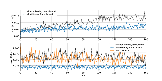
Figure 1: Finite grid instability. Time evolutions of the maximum values of $|A_{z}(0,0,x_{3})|$, and density $n(0,0,x_{3})$.

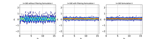
Figure 2: Finite grid instability. The contour plots of the scheme (31) with or without filtering and the scheme (32).

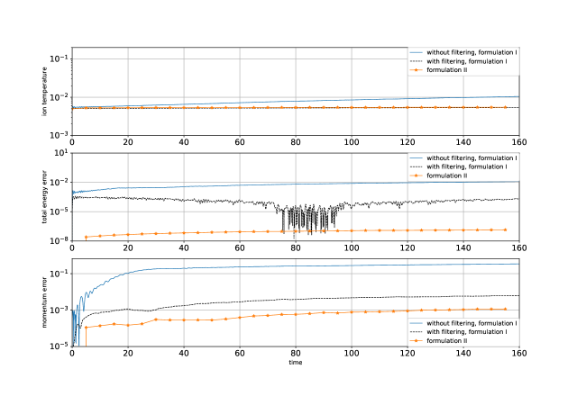
Figure 3: Finite grid instability. Time evolutions of the ion temperature, relative energy error, and momentum error (the third component).

4.2 Parallel electromagnetic wave: R mode

Then we check a parallel propagating R wave by a quasi-1D simulation. Background magnetic field is along $z$ direction. No perturbation is added for the system other than the noises of PIC due to the reduced number of macro-particles. Specifically, the initial conditions we use are:

$${\mathbf{B}}_{0}=(0,0,1),\,{\mathbf{A}}=(0,0,0),\,T=1,\,f=\frac{1}{\pi^{\frac{3}{2}}}e^{-{|{\mathbf{p}}|^{2}}}.$$

Computational parameters are: grid number $[4,4,128]$, domain $[0,1]\times[0,1]\times[0,64]$, $dt=0.005$, final computation time $40$, total particle number $2\times 10^{5}$, degree of B-splines $[3,3,3]$, quadrature point in each cell $[2,2,4]$, and degrees of shape functions $[2,2,2]$. The cell sizes in three directions are $[0.25,0.25,0.5]$, which are small enough to prevent the large errors due to the cancellation problem as pointed in [48] for high-order shape functions. The first order schemes in (31) (without filter or use filters (33) with $m=2$ and coefficients satisfying (34)) and (32) are used. See the numerical results of dispersion relation of R mode given by the scheme (31) in Fig. 4. The black dash lines are the analytical dispersion relations given by Python package HYDRO proposed in [23], when $k\ll 1$, $\omega\propto k$, when $k\gg 1$, $\omega\propto k^{2}$. We can see that our numerical results of the schemes (31)-(32) are in good agreements with the analytical results pretty well even when the wave number $k$ is larger than Nyquist frequency. In Fig. 5, we present the time evolutions of momentum errors and relative energy errors of the schemes (31)-(32), from which we can see the scheme (32) is better than the scheme (31). For the scheme (31), the relative energy error using filters is smaller than the results without filters. The momentum error and relative energy error of the scheme (32) without filter are the smallest, the relative energy error is at the level of $10^{-6}$.

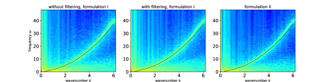
Figure 4: R-waves. The numerical dispersion relations of the R waves given by 1) the scheme (31) without filter, 2) the scheme (31) with filters, 3) the scheme (32).

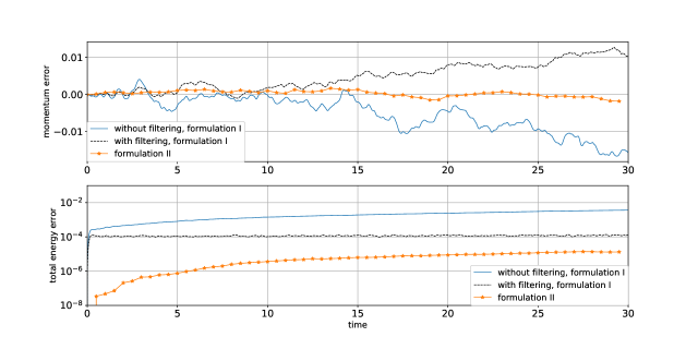
Figure 5: R-waves. Time evolutions of the momentum errors (the third component) and relative energy errors given by 1) the scheme (31) without filter, 2) the scheme (31) with filters, 3) the scheme (32).

4.3 Perpendicular wave: ion Bernstein waves

Then we check Bernstein waves by a one dimensional simulation, which are perpendicular to background magnetic field. In order to excite these waves, we initialize a quasi-1D thermal plasma along the $x$ direction. No initial perturbation is added except the noises of PIC method. Specifically, initial conditions are:

$${\mathbf{B}}_{0}=(0,0,1),\,{\mathbf{A}}=(0,0,0),\ f=\frac{1}{\pi^{\frac{3}{2}}v_{T}^{\frac{3}{2}}}e^{-\frac{|{\mathbf{p}}|^{2}}{v_{T}^{2}}},\,{\color[rgb]{0.1,0.6,0.3}{T}}=0.09.$$

Computational parameters are: grid number $[200,4,4]$, domain $[0,50]\times[0,1]\times[0,1]$, time step size $0.005$, $v_{T}=0.2121$, final computation time $80$, particle number $10^{5}$, degrees of polynomials $[3,3,3]$, quadrature point in each cell $[4,2,2]$, and degrees of shape functions $[2,2,2]$. The first order schemes in (31) (without filter or use filters with $m=3$ and coefficients satisfying (34)) and (32) are used. Firstly, we check the numerical dispersion relations given by the scheme (31) and scheme (32), which are presented in Fig. 6. We can see that both schemes give the correct dispersion relation numerically, the red dashed lines are analytical dispersion relations of Bernstein waves obtained via HYDRO code [23]. All the $n$-th band of the dispersion relation starts close to $n+1$ for small wavenumber and end up at $n$ for large wavenumber. In Fig. 7, we present the momentum errors and relative energy errors of the two schemes. For the scheme (31), the relative energy error and momentum error become smaller when filters are used. The scheme (32) gives best results, the relative energy error is conserved at the level of $10^{-6}$, and the momentum error is around $10^{-2}$.

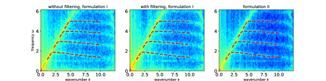
Figure 6: Bernstein waves. Bernstein waves dispersion relation of (a) the scheme (31) without filtering; (b) the scheme (31) with filtering; 3) the scheme (32). Red dash lines are different branches of the analytical dispersion relation of Bernstein waves.

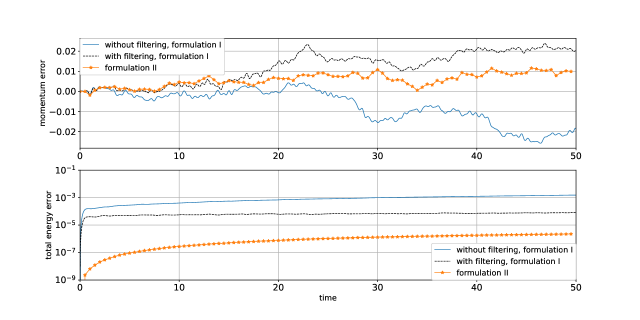
Figure 7: Bernstein waves. Time evolutions of the relative energy errors and momentum errors (the first component) given by the scheme (31) and scheme (32).

4.4 Ion cyclotron instability

Finally we validate the numerical schemes via a nonlinear instability test, ion cyclotron instability. We initialize a quasi-1D thermal plasma along the $x$ direction. No initial perturbation is added except the noises of PIC method. Specifically, initial conditions are:

$${\mathbf{B}}_{0}=(1,0,0),\,{\mathbf{A}}=(0,0,0),\ f=\frac{1}{\pi^{\frac{3}{2}}v_{\parallel}v_{\perp}^{2}}e^{-\frac{p_{x}^{2}}{v_{\parallel}^{2}}-\frac{p_{y}^{2}+p_{z}^{2}}{v_{\perp}^{2}}},\,T=0.5,$$

in which there is a temperature anisotropy. Computational parameters are: grid number $[32,4,4]$, domain $[0,\frac{2\pi}{0.7}]\times[0,1]\times[0,1]$, time step size $0.005$, $v_{\parallel}=1$, $v_{\perp}=2$, final computation time $100$, degrees of polynomials $[3,3,3]$, quadrature point in each cell $[4,2,2]$, and degrees of shape functions $[2,2,2]$. The first order schemes in (31) (without filter or use filters with $m=1$ and coefficients satisfying (34)) and (32) are used.

We present the numerical results of the schemes (31)-(32) using 20000 particles in total in Fig. 8. We can see both schemes give correct exponential growth rates of the Fourier model $\hat{A}_{z}(0.7,0,0)$, 0.2779, which is obtained by using the dispersion relation solver HYDRO code [23]. For the scheme (31) without the filter, the crest of the last oscillations of $|\hat{A}_{z}(0.7,0,0)|$ at about $t=100$ is smallest compared to the results of the scheme (31) with filters and the scheme (32). The scheme (32) gives the smallest momentum error (when time is around 90) and relative energy error. The scheme (31) gives smaller energy error when filters are used.

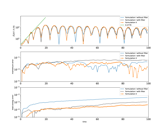
Figure 8: Ion cyclotron instability. Time evolutions of the amplitude of the Fourier mode $\hat{A}_{z}(0.7,0,0)$, momentum error (the first component), and relative energy error with $2\times 10^{4}$ particles.

5 Conclusion

In this work, we explore and compare the canonical momentum based particle-in-cell methods for the two formulations of the hybrid model with kinetic ions and massless electrons. Splitting methods and mid-point rules are used for time discretizations. The schemes of the first formulation are significantly improved by using binomial filters. The schemes of the second formulation show better conservation properties even without filter. Finding more efficient solvers for (25), applying our numerical methods to large scale physical simulations, and numerical comparisons with the schemes constructed in [20] are future works. Smoothed delta functions can also be used in the particle discretizations of all the particle related parts. Let us also mention that other than finite element methods, other methods, such as spectral methods [44] can be used to discretize the vector potential.

6 Appendix

6.1 The hybrid model with a background magnetic field

When there is a background magnetic field ${\mathbf{B}}_{0}$, the formulation I (3) is

$$\frac{\partial f}{\partial t}=-({\mathbf{p}}-{\mathbf{A}})\cdot\frac{\partial f}{\partial{\mathbf{x}}}+\left[\left(\frac{\partial{\mathbf{A}}}{\partial\mathbf{x}}\right)^{\top}({\mathbf{A}}-{\mathbf{p}})\right]\cdot\frac{\partial f}{\partial{\mathbf{p}}}-({\mathbf{p}}-{\mathbf{A}})\times{\mathbf{B}}_{0}\cdot\frac{\partial f}{\partial{\mathbf{p}}},$$

$$\frac{\partial{\mathbf{A}}}{\partial t}=T\frac{\nabla n}{n}-\frac{\nabla\times\left({\mathbf{B}}_{0}+\nabla\times{\mathbf{A}}\right)}{n}\times\left({\mathbf{B}}_{0}+{\nabla\times{\mathbf{A}}}\right)-\frac{\int({\mathbf{A}}-{\mathbf{p}})f\mathrm{d}{\mathbf{p}}}{n}\times\left({{\mathbf{B}}_{0}+\nabla\times{\mathbf{A}}}\right).$$

The formulation II (5) becomes

$$\frac{\partial f}{\partial t}=-({\mathbf{p}}-{\mathbf{A}})\cdot\frac{\partial f}{\partial{\mathbf{x}}}+\left[T\frac{\nabla n}{n}+\left(\frac{\partial{\mathbf{A}}}{\partial\mathbf{x}}\right)^{\top}({\mathbf{A}}-{\mathbf{p}})\right]\cdot\frac{\partial f}{\partial{\mathbf{p}}}-({\mathbf{p}}-{\mathbf{A}})\times{\mathbf{B}}_{0}\cdot\frac{\partial f}{\partial{\mathbf{p}}},$$

$$\frac{\partial{\mathbf{A}}}{\partial t}=-\frac{\nabla\times\left({\mathbf{B}}_{0}+\nabla\times{\mathbf{A}}\right)}{n}\times\left({\mathbf{B}}_{0}+{\nabla\times{\mathbf{A}}}\right)-\frac{\int({\mathbf{A}}-{\mathbf{p}})f\mathrm{d}{\mathbf{p}}}{n}\times\left({{\mathbf{B}}_{0}+\nabla\times{\mathbf{A}}}\right),$$

which could be derived with the following Hamiltonian and anti-symmetric bracket,

$$\mathcal{H}=\frac{1}{2}\int f|{\mathbf{p}}-{\mathbf{A}}|^{2}\mathrm{d}{\mathbf{x}}\mathrm{d}{\mathbf{p}}+T\int n\ln n\mathrm{d}{\mathbf{x}}+\frac{1}{2}\int|\nabla\times{\mathbf{A}}+{\mathbf{B}}_{0}|^{2}\mathrm{d}{\mathbf{x}}.$$

$$\{\mathcal{F},\mathcal{G}\}(f,{\mathbf{A}}) =\int f\left[\frac{\delta\mathcal{F}}{\delta f},\frac{\delta\mathcal{G}}{\delta f}\right]_{xp}\mathrm{d}{\mathbf{x}}\mathrm{d}{\mathbf{p}}-\int\frac{1}{n}\left(\nabla\times\mathbf{A}+{\mathbf{B}}_{0}\right)\cdot\left(\frac{\delta\mathcal{F}}{\delta{\mathbf{A}}}\times\frac{\delta\mathcal{G}}{\delta{\mathbf{A}}}\right)\mathrm{d}{\mathbf{x}}$$

$$+\int f{\mathbf{B}}_{0}\cdot\left(\frac{\partial}{\partial{\mathbf{p}}}\frac{\delta{\mathcal{F}}}{\delta f}\times\frac{\partial}{\partial{\mathbf{p}}}\frac{\delta{\mathcal{G}}}{\delta f}\right)\mathrm{d}{\mathbf{p}}\mathrm{d}{\mathbf{x}}.$$

6.2 $xvA$ formulation

The equivalent hybrid model with unknowns $f(t,{\mathbf{x}}.{\mathbf{v}})$ and ${\mathbf{A}}(t,{\mathbf{x}})$ is

$$\frac{\partial f}{\partial t}+{\mathbf{v}}\cdot\frac{\partial f}{\partial\mathbf{x}}+({\mathbf{E}}+{\mathbf{v}}\times{\mathbf{B}})\cdot\frac{\partial f}{\partial{\mathbf{v}}}=0\,,$$

$$\frac{\partial{\mathbf{A}}}{\partial t}=\left(\mathbf{u}-\frac{\mathbf{J}}{n}\right)\times{\mathbf{B}}\,,$$

$$n=\int f\mathrm{d}{\mathbf{v}},\quad n{\mathbf{u}}=\int{\mathbf{v}}f\mathrm{d}{\mathbf{v}},\quad\mathbf{B}=\nabla\times{\mathbf{A}}\,,$$

$${\mathbf{E}}=-T\frac{\nabla n}{n}-\left(\mathbf{u}-\frac{\mathbf{J}}{n}\right)\times{\mathbf{B}},\quad\mathbf{J}=\nabla\times{\mathbf{B}}.$$

We propose the following anti-symmetric bracket and total energy for this formulation.

$$\{\mathcal{F},\mathcal{G}\}(f,{\mathbf{A}}) =\int f\left[\frac{\delta\mathcal{F}}{\delta f},\frac{\delta\mathcal{G}}{\delta f}\right]_{xv}\mathrm{d}{\mathbf{x}}\mathrm{d}{\mathbf{v}}+\int\frac{\nabla\times{\mathbf{A}}}{\int f\mathrm{d}{\mathbf{v}}}\cdot\frac{\delta\mathcal{F}}{\delta{\mathbf{A}}}\times\frac{\delta\mathcal{G}}{\delta{\mathbf{A}}}\mathrm{d}{\mathbf{x}}$$

$$+\int f\frac{\nabla\times{\mathbf{A}}}{\int f\mathrm{d}{\mathbf{v}}}\cdot\left(\frac{\partial}{\partial{\mathbf{v}}}\frac{\delta\mathcal{G}}{\delta f}\times\frac{\delta\mathcal{F}}{\delta{\mathbf{A}}}-\frac{\partial}{\partial{\mathbf{v}}}\frac{\delta\mathcal{F}}{\delta f}\times\frac{\delta\mathcal{G}}{\delta{\mathbf{A}}}\right)\mathrm{d}{\mathbf{x}}\mathrm{d}{\mathbf{v}}$$

$$+\int\frac{\nabla\times{\mathbf{A}}}{\int f\mathrm{d}{\mathbf{v}}}\cdot\left(\int f\frac{\partial}{\partial{\mathbf{v}}}\frac{\delta\mathcal{F}}{\delta f}\mathrm{d}{\mathbf{v}}\right)\times\left(\int f\frac{\partial}{\partial{\mathbf{v}}^{\prime}}\frac{\delta\mathcal{G}}{\delta f}\mathrm{d}{\mathbf{v}}^{\prime}\right)\mathrm{d}{\mathbf{x}}$$

$$+\int f\left(\nabla\times{\mathbf{A}}\cdot\frac{\partial}{\partial{\mathbf{v}}}\frac{\delta\mathcal{F}}{\delta f}\times\frac{\partial}{\partial{\mathbf{v}}}\frac{\delta\mathcal{G}}{\delta f}\right)\mathrm{d}{\mathbf{x}}\mathrm{d}{\mathbf{v}},$$

$$\mathcal{H}=\frac{1}{2}\int|{\mathbf{v}}|^{2}f\,\textnormal{d}{\mathbf{x}}\textnormal{d}{\mathbf{v}}+\frac{1}{2}\int|\nabla\times{\mathbf{A}}|^{2}\,\textnormal{d}{\mathbf{x}}\,+T\int\left(\int f\,\textnormal{d}\mathbf{v}\right)\ln\left(\int f\,\textnormal{d}\mathbf{v}\right)\textnormal{d}{\mathbf{x}}.$$

Energy conserving particle-in-cell methods for the $xvA$ formulation can be constructed following the strategies proposed in [12, 20].

References

- [1] Kraus M, Kormann K, Morrison P J, Sonnendrücker E. GEMPIC: geometric electromagnetic particle-in-cell methods. Journal of Plasma Physics, 2017, 83(4).
- [2] Qin H, Liu J, Xiao J, Zhang R, He Y, Wang Y, Sun Y, Burby J W, Ellison L, Zhou Y. Canonical symplectic particle-in-cell method for long-term large-scale simulations of the Vlasov–Maxwell equations. Nuclear Fusion, 2015, 56(1): 014001.
- [3] Tronci C. Hamiltonian approach to hybrid plasma models. Journal of Physics A, 2010, 43(37).
- [4] Xiao J, Qin H, Liu J, He Y, Zhang R, Sun Y. Explicit high-order non-canonical symplectic particle-in-cell algorithms for Vlasov-Maxwell systems. Physics of Plasmas, 2015, 22(11): 112504.
- [5] Feng K, Qin M. Symplectic geometric algorithms for Hamiltonian systems. Berlin: Springer, 2010.
- [6] Holderied F, Possanner S, Wang X. MHD-kinetic hybrid code based on structure-preserving finite elements with particles-in-cell. Journal of Computational Physics, 2021, 433: 110143.
- [7] Xiao J, Qin H. Field theory and a structure-preserving geometric particle-in-cell algorithm for drift wave instability and turbulence. Nuclear Fusion, 2019, 59(10): 106044.
- [8] Birdsall C K, Langdon A B. Plasma physics via computer simulation. CRC press, 2018.
- [9] Hairer E, Lubich C, Wanner G. Geometric Numerical Integration: Structure-Preserving Algorithms for Ordinary Differential Equations, vol. 31, Springer Science & Business Media, 2006.
- [10] Arnold D N, Falk R S, Winther R. Finite element exterior calculus, homological techniques, and applications. Acta numerica, 2006, 15: 1-155.
- [11] Hirani A N. Discrete exterior calculus. California Institute of Technology, 2003.
- [12] Kormann K, Sonnendrücker E. Energy-conserving time propagation for a structure-preserving particle-in-cell Vlasov–Maxwell solver. Journal of Computational Physics, 2020, 425: 109890.
- [13] He Y, Sun Y, Qin H, Liu J. Hamiltonian particle-in-cell methods for Vlasov–Maxwell equations. Physics of Plasmas, 2016, 23(9): 092108.
- [14] Kelley C T. Iterative methods for linear and nonlinear equations. Society for Industrial and Applied Mathematics, 1995.
- [15] Gonzalez O. Time integration and discrete Hamiltonian systems. Journal of Nonlinear Science, 1996, 6(5): 449-467.
- [16] Kaltsas D A, Throumoulopoulos G N, Morrison P J. Hamiltonian kinetic-Hall magnetohydrodynamics with fluid and kinetic ions in the current and pressure coupling schemes. Journal of Plasma Physics, 2021, 87(5): 835870502.
- [17] Matthews A P. Current advance method and cyclic leapfrog for 2D multispecies hybrid plasma simulations. Journal of Computational Physics, 1994, 112(1): 102-116.
- [18] Franci L, Hellinger P, Guarrasi M, Chen C H K, Papini E, Verdini A, Matteini L, Landi S. Three-dimensional simulations of solar wind turbulence with the hybrid code CAMELIA. Journal of Physics: Conference Series. IOP Publishing, 2018, 1031(1): 012002.
- [19] Valentini F, Trávníček P, Califano F, Hellinger P, Mangeney A. A hybrid-Vlasov model based on the current advance method for the simulation of collisionless magnetized plasma. Journal of Computational Physics, 2007, 225(1): 753-770.
- [20] Li Y, Campos Pinto M, Holderied F, Possanner S, Sonnendrücker E. Geometric Particle-In-Cell discretizations of a plasma hybrid model with kinetic ions and mass-less fluid electrons, submitted.
- [21] Stanier A, Chacón L, Chen G. A fully implicit, conservative, non-linear, electromagnetic hybrid particle-ion/fluid-electron algorithm. Journal of Computational Physics, 2019, 376: 597-616.
- [22] Stanier A, Chacón L. A conservative implicit-PIC scheme for the hybrid kinetic-ion fluid-electron plasma model on curvilinear meshes. Journal of Computational Physics, 2022, 459: 111144.
- [23] Told D, Cookmeyer J, Astfalk P, Jenko F. A linear dispersion relation for the hybrid kinetic-ion/fluid-electron model of plasma physics. New Journal of Physics, 2016, 18(7): 075001.
- [24] Kunz M W, Stone J M, Bai X N. Pegasus: a new hybrid-kinetic particle-in-cell code for astrophysical plasma dynamics. Journal of Computational Physics, 2014, 259: 154-174.
- [25] Vay J L, Geddes C G R, Cormier-Michel E, Grote D P. Numerical methods for instability mitigation in the modeling of laser wakefield accelerators in a Lorentz-boosted frame. Journal of Computational Physics, 2011, 230(15): 5908-5929.
- [26] Rambo P W. Finite-grid instability in quasineutral hybrid simulations. Journal of Computational Physics, 1995, 118(1): 152-158.
- [27] Lipatov A S. The hybrid multiscale simulation technology: an introduction with application to astrophysical and laboratory plasmas. Springer Science & Business Media, 2002.
- [28] Park W, Parker S, Biglari H, et al. Three-dimensional hybrid gyrokinetic-magnetohydrodynamics simulation. Physics of Fluids B: Plasma Physics, 1992, 4(7): 2033-2037.
- [29] Winske D, Yin L, Omidi N, Karimabadi H, Quest K. Hybrid simulation codes: Past, present and future–A tutorial. Space plasma simulation, 2003: 136-165.
- [30] Perse B, Kormann K, Sonnendrücker E. Perfect Conductor Boundary Conditions for Geometric Particle-in-Cell Simulations of the Vlasov–Maxwell System in Curvilinear Coordinates. arXiv preprint arXiv:2111.08342, 2021.
- [31] McLachlan R I, Quispel G R W, Robidoux N. Geometric integration using discrete gradients. Philosophical Transactions of the Royal Society of London. Series A: Mathematical, Physical and Engineering Sciences, 1999, 357(1754): 1021-1045.
- [32] Zhang R, Qin H, Tang Y, Liu J, He Y, Xiao J. Explicit symplectic algorithms based on generating functions for charged particle dynamics. Physical Review E, 2016, 94(1): 013205.
- [33] Zhou Z, He Y, Sun Y, Liu J, Qin H. Explicit symplectic methods for solving charged particle trajectories. Physics of Plasmas, 2017, 24(5): 052507.
- [34] Haggerty C C, Caprioli D. dHybridR: A hybrid particle-in-cell code including relativistic ion dynamics. The Astrophysical Journal, 2019, 887(2): 165.
- [35] Campos Pinto M, Kormann K, Sonnendrücker E. Variational framework for structure-preserving electromagnetic particle-in-cell methods. Journal of Scientific Computing, 2022, 91(2): 1-39.
- [36] Winske D. Hybrid simulation codes with application to shocks and upstream waves. Space Science Reviews, 1985, 42(1): 53-66.
- [37] Winske D, Karimabadi H, Le A, Omidi N, Roytershteyn V, Stanier A. Hybrid codes (massless electron fluid). arXiv preprint arXiv:2204.01676, 2022.
- [38] Chen L, White R B, Rosenbluth M N. Excitation of internal kink modes by trapped energetic beam ions. Physical Review Letters, 1984, 52(13): 1122.
- [39] Coppi B, Porcelli F. Theoretical model of fishbone oscillations in magnetically confined plasmas. Physical review letters, 1986, 57(18): 2272.
- [40] Park W, Belova E V, Fu G Y, Tang X Z, Strauss H R, Sugiyama L E. Plasma simulation studies using multilevel physics models. Physics of Plasmas, 1999, 6(5): 1796-1803.
- [41] Hahm T S, Lee W W, Brizard A. Nonlinear gyrokinetic theory for finite-beta plasmas. The Physics of fluids, 1988, 31(7): 1940-1948.
- [42] Mishchenko A, Cole M, Kleiber R, Könies A. New variables for gyrokinetic electromagnetic simulations. Physics of Plasmas, 2014, 21(5).
- [43] Bao J, Liu D, Lin Z. A conservative scheme of drift kinetic electrons for gyrokinetic simulation of kinetic-MHD processes in toroidal plasmas. Physics of Plasmas, 2017, 24(10).
- [44] Campos Pinto M, Ameres J, Kormann K, Sonnendrücker E. On geometric Fourier particle in cell methods. arXiv preprint arXiv:2102.02106, 2021.
- [45] Servidio S, Valentini F, Califano F, Veltri P. Local kinetic effects in two-dimensional plasma turbulence. Physical review letters, 2012, 108(4): 045001.
- [46] Kunz M W, Schekochihin A A, Stone J M. Firehose and mirror instabilities in a collisionless shearing plasma. Physical Review Letters, 2014, 112(20): 205003.
- [47] Arzamasskiy L, Kunz M W, Chandran B D G, Quataert E. Hybrid-kinetic simulations of ion heating in Alfvénic turbulence. The Astrophysical Journal, 2019, 879(1): 53.
- [48] Stanier A, Chacon L, Le A. A cancellation problem in hybrid particle-in-cell schemes due to finite particle size. Journal of Computational Physics, 2020, 420: 109705.
- [49] Crouseilles N, Einkemmer L, Faou E. Hamiltonian splitting for the Vlasov–Maxwell equations. Journal of Computational Physics, 2015, 283: 224-240.
- [50] Qin H, He Y, Zhang R, Liu J, Xiao J, Wang Y. Comment on "Hamiltonian splitting for the Vlasov–Maxwell equations". Journal of Computational Physics, 2015, 297: 721-723.
- [51] He Y, Qin H, Sun Y, Xiao J, Zhang R, Liu J. Hamiltonian time integrators for Vlasov–Maxwell equations. Physics of Plasmas, 2015, 22(12).