Margolus-Levitin quantum speed limit for an arbitrary fidelity
Abstract
The Mandelstam-Tamm and Margolus-Levitin quantum speed limits are two well-known evolution time estimates for isolated quantum systems. These bounds are usually formulated for fully distinguishable initial and final states, but both have tight extensions to systems that evolve between states with an arbitrary fidelity. However, the foundations of these extensions differ in some essential respects. The extended Mandelstam-Tamm quantum speed limit has been proven analytically and has a clear geometric interpretation. Furthermore, which systems saturate the limit is known. The derivation of the extended Margolus-Levitin quantum speed limit, on the other hand, is based on numerical estimates. Moreover, the limit lacks a geometric interpretation, and no complete characterization of the systems reaching it exists. In this paper, we derive the extended Margolus-Levitin quantum speed limit analytically and describe the systems that saturate the limit in detail. We also provide the limit with a symplectic-geometric interpretation, which indicates that it is of a different character than most existing quantum speed limits. At the end of the paper, we analyze the maximum of the extended Mandelstam-Tamm and Margolus-Levitin quantum speed limits and derive a dual version of the extended Margolus-Levitin quantum speed limit. The maximum limit is tight regardless of the fidelity of the initial and final states. However, the conditions under which the maximum limit is saturated differ depending on whether or not the initial state and the final state are fully distinguishable. The dual limit is also tight and follows from a time reversal argument. We describe the systems that saturate the dual quantum speed limit.
I Introduction
A quantum speed limit (QSL) is a lower bound on the time it takes to transform a quantum system in some predetermined way. QSLs exist for all sorts of transformations of both open and closed systems. Many involve statistical quantities such as energy, entropy, fidelity, and purity [1, 2, 3, 4, 5].
A prominent QSL is attributed to Mandelstam and Tamm [6]. The Mandelstam-Tamm QSL states that the time it takes for an isolated quantum system to evolve between two fully distinguishable states is at least divided by the energy uncertainty,111In this paper, “state” refers to a pure quantum state unless otherwise is explicitly stated.,222Two states are fully distinguishable if their fidelity is zero.,333All quantities are expressed in units such that .
| (1) |
Mandelstam and Tamm actually showed a more general result: If the fidelity between the initial state and the final state is , the evolution time is bounded according to
| (2) |
Anandan and Aharonov [7] provided the Mandelstam-Tamm QSL with an elegant geometric interpretation when they showed that the Fubini-Study distance between two states with fidelity is and that the Fubini-Study evolution speed equals the energy uncertainty. Inequality (2) is thus saturated for isolated systems where the state evolves along a shortest Fubini-Study geodesic. Anandan and Aharonov’s work inspired the writing of Ref. [8], which extends the Mandelstam-Tamm QSL to systems in mixed states in several different ways.
Margolus and Levitin [9] derived another QSL that is often mentioned together with Mandelstam and Tamm’s. The Margolus-Levitin QSL states that the time it takes for an isolated quantum system to evolve between two fully distinguishable states is at least divided by the expected energy shifted by the smallest energy,
| (3) |
Giovannetti et al. [10] extended Margolus and Levitin’s QSL to an arbitrary fidelity. More precisely, they showed that the evolution time of an isolated system is bounded from below according to
| (4) |
where is a function that depends only on the fidelity between the initial and final states; see Sec. II. Giovannetti et al. also showed that (4), like (2), is tight, which means that for each there is a system for which the inequality in (4) is an equality. However, apart from that, the situation is different from the case of the Mandelstam-Tamm QSL: A closed formula for does not exist, the derivation of (4) rests on numerical estimates, there is no classification of the systems saturating (4), and a geometric interpretation like that of (2) is lacking [1, 2, 11, 12].
In this paper, we derive the extended Margolus-Levitin QSL analytically and characterize the systems that saturate this estimate (Sec. II). Furthermore, we show that the extended Margolus-Levitin QSL has a symplectic-geometric interpretation and is connected to the Aharonov-Anandan geometric phase [13] (Sec. III). The Margolus-Levitin QSL thus differs fundamentally from most existing QSLs. That the estimates in (3) and (4) are either invalid or correct but not tight unless we shift the expected energy with the smallest energy suggests that a ground state will play a central role in the derivation of the extended Margolus-Levitin QSL and in its geometric interpretation.
The maximum of the Mandelstam-Tamm and the extended Margolus-Levitin QSL is also a QSL. The characteristics of the maximum QSL differ depending on whether or not the initial state and final state are fully distinguishable. We explain why this is so, and we provide several QSLs that are related to but less sharp than the extended Margolus-Levitin QSL. We also derive a dual version of the extended Margolus-Levitin QSL involving the largest rather than the smallest energy (Sec. IV). The paper concludes with a summary and a comment on the difficulty of extending the Margolus-Levitin quantum speed limit to driven systems (Sec. V). For a more detailed discussion of this difficulty, see Ref. [14].
II The extended Margolus-Levitin quantum speed limit
The function in Giovannetti et al.’s estimate (4) is444The in Ref. [10] equals the in (5) multiplied by .
| (5) |
For each , the minimum on the right-hand side is assumed for a unique . Figure 1 shows the graph of .
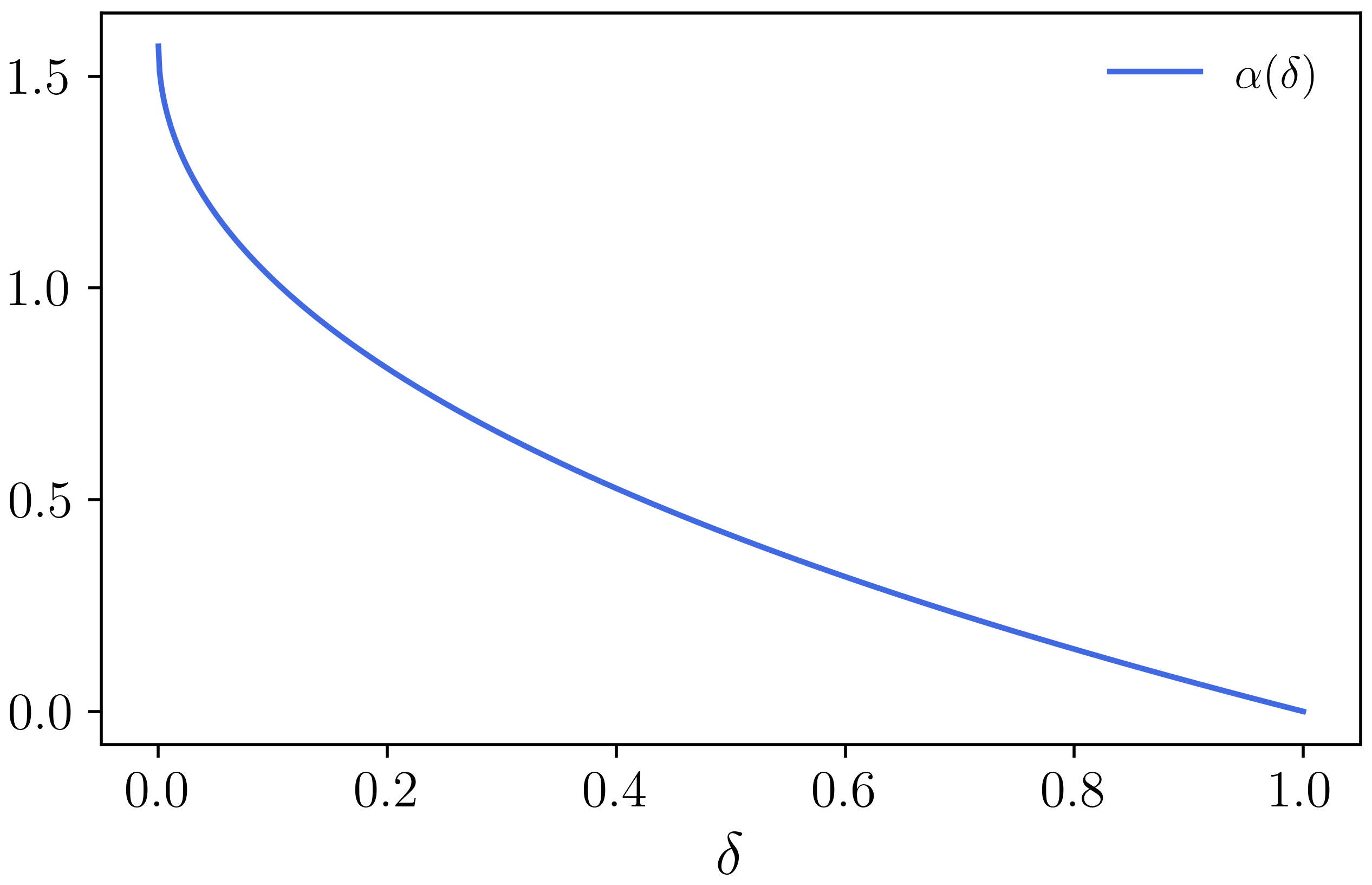
Note that depends only on the fidelity between the initial and final states. The fidelity, or overlap, between two pure states and is .
Although the Margolus-Levitin QSL (3) is quite surprising, its proof is relatively simple [9]. Giovannetti et al.’s estimate (4) reduces to the Margolus-Levitin QSL for , but the derivation in Ref. [10] for a general is rather complicated. Moreover, it is partly based on numerical calculations. In this section, we derive (4) analytically. We also characterize the systems, that is, the states and Hamiltonians that saturate (4).
For simplicity, we write for the expected energy of a system without reference to its state. Furthermore, we write for the difference between and the smallest eigenvalue of . We call this quantity the normalized expected energy. In this paper we only consider isolated systems, that is, systems where a time-independent Hamiltonian governs the dynamics. For such systems, the expected energy and normalized expected energy are conserved quantities. The expected energy and normalized expected energy thus depend on the initial state but do not change as the state evolves.
II.1 The extended Margolus-Levitin quantum speed limit for a two-dimensional system
In this section we show that Giovannetti et al.’s estimate (4) is valid and tight for qubit systems. Derivations of the statements in this section can be found in Appendix A.
Consider a qubit system with Hamiltonian
| (6) |
the vectors and being orthonormal. We identify each qubit state with a unit length vector called the Bloch vector of by defining
| (7) | ||||
| (8) | ||||
| (9) |
The dynamics induced by causes the Bloch vectors to rotate about the axis with a constant inclination and an azimuthal angular speed . Furthermore, a state’s expected energy is determined by, and determines, the coordinate of its Bloch vector:
| (10) |
Two states thus have the same expected energy if and only if their Bloch vectors have the same coordinate.
Let and be the Bloch vectors of two states with a common coordinate and fidelity , and suppose that causes to rotate to in time . Using (7)–(9) one can show that the inner product between and relates to the fidelity as
| (11) |
To determine the distance traveled by the rotating Bloch vector consider the orthogonal projections and of and on the plane. During the evolution, rotates to along the peripheral arc of a circular sector in the plane of radius and apex angle . The distance traveled by the rotating Bloch vector equals the length of the peripheral arc and is, thus,
| (12) |
The speed of the rotating Bloch vector is , and hence, by (12), the evolution time is
| (13) |
Combined with (10), this gives that
| (14) |
The relation (11) implies that the coordinate squared of the Bloch vectors of two states with the same expected energy is less than the fidelity between the states:
| (15) |
Conversely, each expected energy level corresponding to a such that contains Bloch vectors of states with fidelity . We conclude that for a qubit. Equality holds if and only if the coordinate of the Bloch vector of the initial state minimizes the right side of (14) over the interval and thus is such that
| (16) |
II.2 The extended Margolus-Levitin quantum speed limit for systems of arbitrary dimension
Section II.1 shows that Giovannetti et al.’s estimate (4) is valid and tight for qubit systems. Section II.1 also shows that for an arbitrary isolated system with Hamiltonian there is a state that evolves into one with fidelity in such a way that (4) is an identity: Let and be eigenvectors of with eigenvalues and , with . Choose a with support in the span of and and such that defined by (9) satisfies (16). Then will evolve to a state with fidelity in time . Conversely, for any system in a state , a Hamiltonian exists that transforms into a state with fidelity in such a way that (4) is saturated: Take an whose sum of two eigenspaces, one of which corresponds to its smallest eigenvalue , contains the support of . Adjust ’s spectrum so that defined by (9) satisfies (16). Then will evolve to a state with fidelity in time .
An effective qubit for is a state with support in the sum of two eigenspaces of . It behaves like a genuine qubit in that its support evolves in the linear span of two energy eigenvectors, one from each eigenspace covering the initial support. The above discussion shows that (4) holds for and can always be saturated by an effective qubit. We say that a state is partly grounded if the eigenspace corresponding to is not contained in the kernel of the state or, equivalently, if the eigenspace of is not orthogonal to the support of the state. In Appendix B we show the first main result of this paper: If assumes its smallest possible value when evaluated for all Hamiltonians , states , and such that transforms into a state with fidelity in time , then is a partly grounded effective qubit for and . The extended Margolus-Levitin QSL (4) thus holds generally and is a tight estimate saturable in all dimensions. We interpret (4) geometrically in Sec. III. There we see, among other things, that one can interpret as an extremal dynamical phase. Notice the contrast with the Mandelstam-Tamm QSL, where the numerator is a geodesic distance.
Remark 1.
If we select a subset of the spectrum of and consider only initial states with support in the sum of the eigenspaces of the eigenvalues in the subset, then the support of the evolved state will remain in that sum. The proof in Appendix B shows that the evolution time of each such state satisfies the inequality
| (17) |
with being the smallest eigenvalue in the subset.555To avoid having to treat trivial cases separately, we assume that the subset contains at least two different eigenvalues. Furthermore, by Sec. II.1, inequality (17) can be saturated with an effective qubit that evolves in the sum of the eigenspaces corresponding to two eigenvalues in the subset, one of which is . As a special case, we have that the evolution time is bounded according to
| (18) |
where is the smallest occupied energy, that is, the smallest eigenvalue of whose corresponding eigenspace is not annihilated by . Often, the Margolus-Levitin QSL is formulated with the expected energy shifted by the smallest occupied energy rather than the smallest energy. Mathematically, however, there is no difference because we can always reduce the Hilbert space to an effective Hilbert space and consider the smallest occupied energy as the smallest energy. (However, see Remark 2.)
Remark 2.
The state must evolve in the span of two eigenvectors of to saturate (4), one of which has eigenvalue . No requirements are placed on the eigenvalue of the second eigenvector except that it must differ from . However, if we want the evolution time to be as short as possible, must be the largest eigenvalue of . This follows from (10) since saturation of (4) implies that the quotient is independent of . Thus, the maximum value of , and consequently the minimum value of , is obtained for the maximizing the difference . The observation that the state that saturates (4) with the shortest possible evolution time is an effective qubit with support in the sum of the eigenspaces belonging to the largest and the smallest eigenvalue generalizes the main result in Ref. [15] to arbitrary fidelity; see also Ref. [16]. A corresponding statement holds if we restrict the Hilbert space as in Remark 1.
In contrast to the energy uncertainty, we cannot consider the normalized expected energy as a measure of a state’s rate of change. Since for each state there exist Hamiltonians and , with smallest eigenvalues and , that identically evolve the state but for which and are different. Thus, unlike most QSLs, the extended Margolus-Levitin QSL is not a quotient of a distance and a speed [1, 2, 11, 12].
III Geometry of the extended Margolus-Levitin quantum speed limit
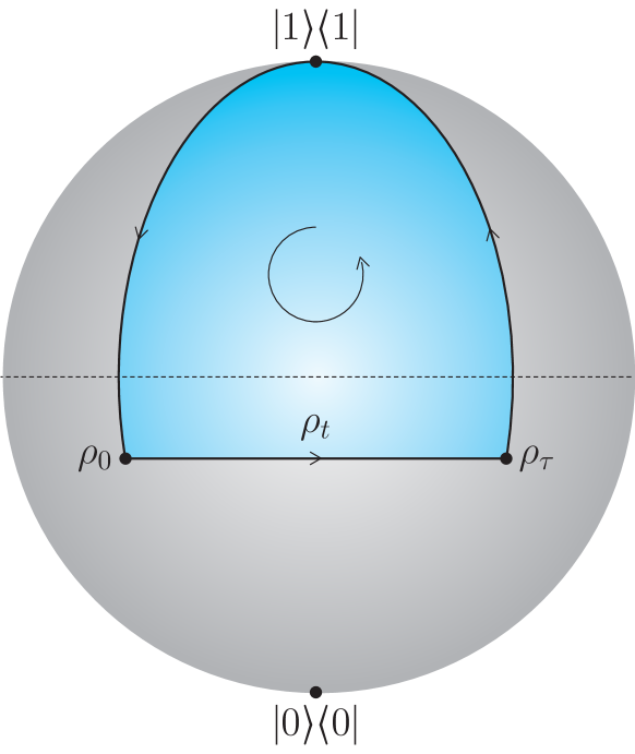
Equations (7)–(9) describe a diffeomorphism between the projective Hilbert space of qubit states and the Bloch sphere. (Thus, we can identify qubit states with their corresponding Bloch vectors.) We push forward the Fubini-Study Riemannian metric and symplectic form using this diffeomorphism.666The Fubini-Study distance is equal to half of the standard distance function on the unit sphere, and the Fubini-Study symplectic form is equal to half the standard area form on the unit sphere. The expression in (14) is then the negative of the symplectic area of a surface with a triangular boundary in the Bloch sphere. The path traced out by the evolving state and the shortest geodesics connecting the initial and final state to the lowest energy state form the boundary of the surface; see Fig. 2.

Notice that we have oriented the boundary so that the surface has the reverse orientation compared with the standard orientation of the Bloch sphere. In Sec. III.2, we show that is equal to the negative of the symplectic area of such a triangular surface also in the general case.
The expected energy level to which the initial qubit state belongs is a geodesic sphere centered at , that is, a sphere made up of all states at a fixed distance from . The radius of the geodesic sphere is
| (19) |
Therefore, . If we substitute for on the right-hand side of (5) we get
| (20) |
where ranges from to . Section III.3 shows that the expression minimized on the right-hand side is an extremal dynamical phase in a gauge specified by a stationary state with eigenvalue . First, in Sec. III.1, we interpret as a dynamical phase.
III.1 Evolution time times normalized expected energy as a dynamical phase
Consider a quantum system modeled on a finite-dimensional Hilbert space . Let be the unit sphere in and be the projective Hilbert space of orthogonal projection operators of rank on .777Such operators represent pure states. The Hopf bundle is the -principal bundle that sends each in to the corresponding state in . The Berry connection on the Hopf bundle is defined as
| (21) |
on tangent vectors at .
Assume the system has a Hamiltonian . Choose an eigenstate of with eigenvalue . Let be the open neighborhood of consisting of all states that are not fully distinguishable from . Hypersurfaces in , one for each vector in the fiber over , foliate the preimage of under ; see Fig. 3 and Ref. [17].
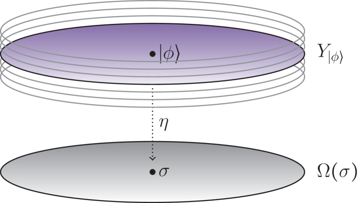
The hypersurface consists of all vectors in that are in phase with , that is, are such that . The gauge group permutes the hypersurfaces, and maps each hypersurface diffeomorphically onto . We can thus define a gauge potential on by pushing down the restriction of to an arbitrary hypersurface . The potential depends on but not on the choice of in the fiber over .
The second main result in the paper reads: If is a state in , and , where , is the evolution curve starting from , then is contained in and
| (22) |
In other words, is the dynamical phase of in a gauge associated with .888Some authors call the negative of the right-hand side of (22) the dynamical phase of . To prove (22) select a in the fiber over , let be the vector over in phase with , and let be the curve that extends from and has the velocity field . The curve is in phase with and projects to :
| (23) | |||
| (24) |
Hence,
| (25) |
Notice that if is a ground state.
III.2 Evolution time times normalized expected energy as the negative of a symplectic area
We equip the projective Hilbert space with the Fubini-Study Riemannian metric and symplectic form . For tangent vectors and at ,999We normalize and asymmetrically as this gives rise to cleaner formulas.
| (26) | |||
| (27) |
The geodesic distance function associated with the Fubini-Study metric is
| (28) |
Suppose the system is in a state and a Hamiltonian governs its dynamics. Let , , represent the evolving state. Since is time-independent, the distances between and the eigenstates of are preserved. Let be an eigenstate with eigenvalue located at a distance from . Furthermore, let and be the shortest unit speed geodesics from to and from to , respectively. The closure of is the concatenation defined as
| (29) |
The left part of Fig. 4 illustrates the closure.
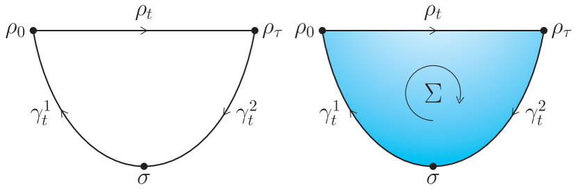
Below we show the third main result of the paper:
| (30) |
where is any Seifert surface for that is homologous to a Seifert surface for in . A Seifert surface for is an oriented surface in whose boundary is parametrized by as illustrated in the right part of Fig. 4. For example, the ruled surface obtained by connecting and each with the shortest arclength-parametrized geodesic is such a Seifert surface. In Appendix C we provide formulas for the geodesics and and explicitly construct a ruled Seifert surface for .
The pull-back of to by the Hopf projection is exact and equals the negative of the Berry curvature, [17]. We construct a lift of to as follows. Let be any vector in the fiber over , let be the lift of which is in phase with , and for define and as
| (31) | |||
| (32) |
The curves and are lifts of and connecting to and to , respectively; see Appendix C. We define as the concatenation . The curve is a lift of that is in phase with .
Suppose that is homologous to a Seifert surface in . The Hopf bundle restricts to a diffeomorphism from the hypersurface of vectors in that are in phase with onto [17]. Lift to a Seifert surface for in . By Stoke’s theorem,
| (33) |
The first identity is a consequence of being a homological boundary and that is closed; cf. Remark 3 below. The second identity results from being a diffeomorphism from onto and being the pull-back of . The third identity follows from parametrizing the boundary of the lift of .
A direct calculation shows that the Berry connection annihilates the velocity fields of and :
| (34) |
Thus we have that
| (35) |
Equations (25), (33), and (35) yield the third main result (30). Note that the calculations rely on not being fully distinguishable from , cf. Remark 1.
Remark 3.
The homology class of the projectivization of any two-dimensional subspace of , that is, a Bloch sphere, generates the second singular homology group of with integer coefficients [18]. We choose such a Bloch sphere that we orient so that its symplectic area is positive. The area is , and is thus of integral class.
The difference between two Seifert surfaces for is a -cycle. The homology class of such a difference is an integer multiple of the homology class for the Bloch sphere. It follows that the difference of the symplectic areas of two Seifert surfaces for is an integer multiple of the symplectic area of the Bloch sphere. Hence, for an arbitrary Seifert surface for ,
| (36) |
We can equivalently express this as being equal to the Aharonov-Anandan geometric phase [13] of the closure of modulo . This connection to the Aharonov-Anandan phase is utilized in Ref. [19] where QSLs for cyclic systems are derived.
III.3 as an extremal dynamical phase
Let be any state and be the geodesic sphere of radius centered at . The geodesic sphere consists of all states at distance from . Fix a fidelity and choose such that . The geodesic sphere is then contained in and includes states between which the fidelity is .
Write for the space of smooth curves in that extend between two states with fidelity . Define to be the functional that assigns the dynamical phase to each in in the gauge specified by ,
| (37) |
In Appendix D we show that is an extremal for if and only if for every in the fiber over , the lift of which is in phase with splits orthogonally as
| (38) |
for some function that vanishes for . The corresponding extreme value is
| (39) |
The constraint on arising from the assumption that extends between two states with fidelity reads
| (40) |
Thus,
| (41) |
According to (20), is equal to the smallest positive extreme value of minimized over the interval . This observation is the fourth main result of the paper.
IV Related quantum speed limits
The maximum of the Mandelstam-Tamm and the extended Margolus-Levitin QSLs is a new QSL. Interestingly, the maximum QSL behaves differently for fully and not fully distinguishable initial and final states. We describe this difference in Sec. IV.1. In Sec. IV.2 we derive a QSL that extends the dual Margolus-Levitin QSL studied in Ref. [20], and in Sec. IV.3 we provide three QSLs that are less sharp but easier to calculate than the extended Margolus-Levitin QSL. These three QSLs are not new but can be found in the cited papers.
IV.1 The maximum quantum speed limit
According to Anandan and Aharonov [7], the QSL of Mandelstam and Tamm (2) is saturated if and only if the evolving state follows a shortest Fubini-Study geodesic. Furthermore, by Brody [21], such a state is an effective qubit that follows the equator of the Bloch sphere associated with the two eigenvectors that have nonzero fidelity with the initial state; cf. Sec. II.1.101010None of the eigenvectors need to be associated with the smallest eigenvalue of the Hamiltonian. Levitin and Toffoli [16] showed that if we require the initial and final states to be fully distinguishable, the same holds for the Margolus-Levitin QSL (3). However, in that case, one of the eigenvectors must belong to the smallest eigenvalue (or be replaced by the smallest occupied energy, cf. Remark 1). Thus, if (3) is saturated, so is (1), and the reverse holds if the support of the initial state is not perpendicular to the eigenspace belonging to the smallest eigenvalue. These observations led Levitin and Toffoli to conclude that the maximum of and is a tight lower bound for the evolution time only reachable for states such that . We can draw the same conclusion from the discussion in Sec. II.
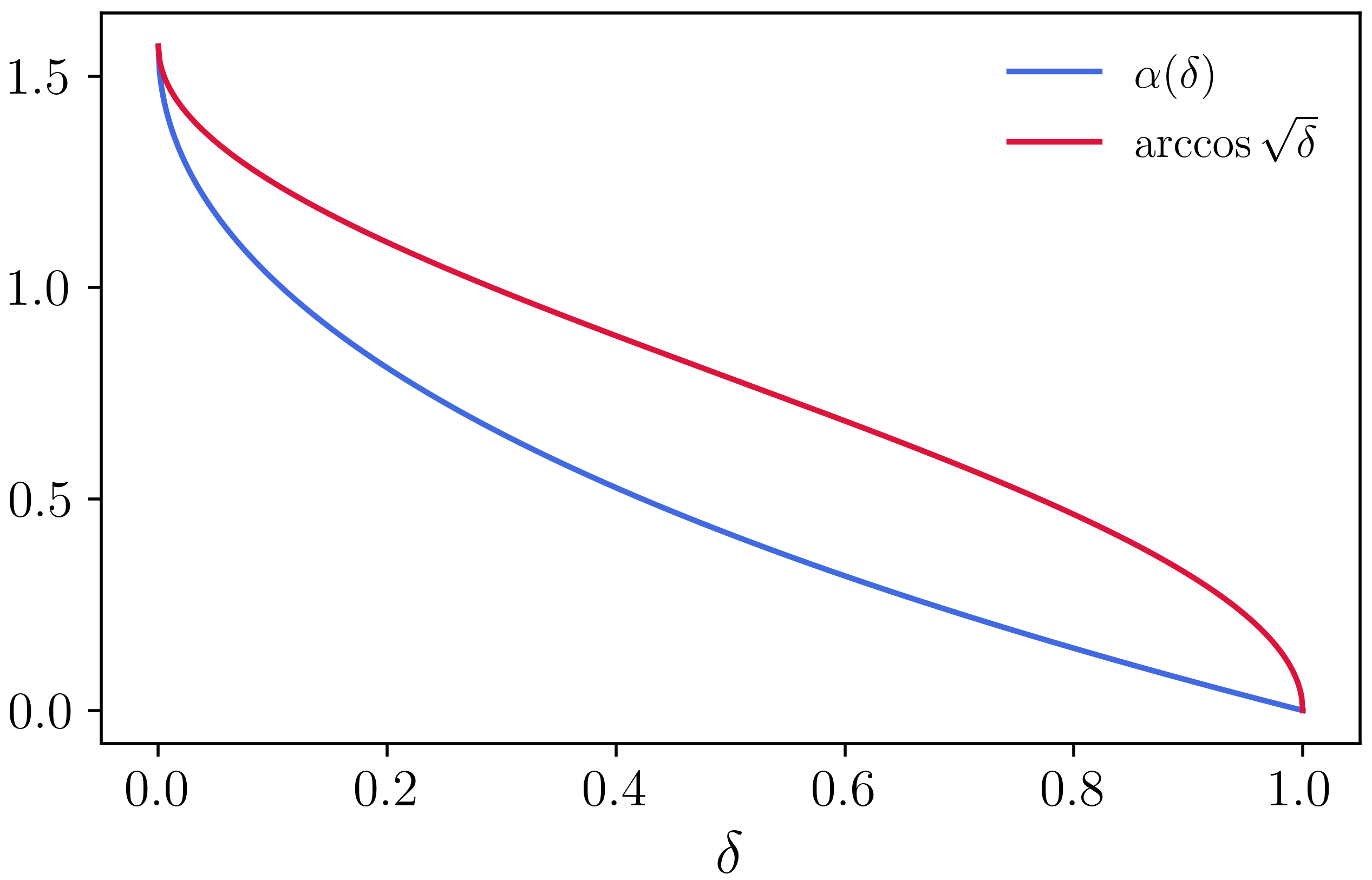
Interestingly, the situation is almost the reverse for a nonzero fidelity between initial and final states; the Mandelstam–Tamm and the extended Margolus–Levitin QSLs can never saturate simultaneously: If the state follows a geodesic, then (4) is not saturated by Sec. II.1, and if (4) is an identity, the state does not follow a geodesic. However, the maximum QSL can be reached: If the state follows a geodesic, , and if condition (16) is satisfied, . In the latter case, must differ from since is strictly less than for ; see Fig. 5.
Remark 5.
The state does not follow a geodesic in a system that saturates the extended Margolus-Levitin QSL for a nonzero fidelity. However, the state follows a sub-Riemannian geodesic in a geodesic sphere centered at a ground state. See Appendix C for details.
Remark 6.
In quite a few papers it is claimed that is a QSL for isolated systems. Figure 5 and the fact that the extended Margolus-Levitin QSL is tight show that this is not true in general.
IV.2 The dual extended Margolus-Levitin quantum speed limit
Let and be states with fidelity , and suppose that evolves to in time . Then evolves to in time . The smallest eigenvalue of is , where is the largest eigenvalue of , and according to the extended Margolus-Levitin QSL,
| (42) |
This estimate generalizes the main result in Ref. [20] to an arbitrary fidelity between initial and final states. We adhere to the terminology in Ref. [20] and call the dual extended Margolus-Levitin QSL. Note that for some states, is greater than and .
Since the estimate in (42) is a consequence of applying the extended Margolus-Levitin QSL to evolution generated by , it follows from Appendix B that (42) can be saturated in all dimensions and that, when so, the state is an effective qubit for whose support is not orthogonal to the eigenspace corresponding to . But then the state is also an effective qubit for whose support is not orthogonal to the eigenspace corresponding to . We call such an effective qubit partly maximally excited. To summarize, if assumes its smallest possible value when evaluated for all Hamiltonians , states , and such that transforms into a state with fidelity in time , then is a partly maximally excited effective qubit for and .
Remark 7.
If we restrict the set of states as in Remark 1, can be replaced by the largest occupied energy.
The discussion in Sec. III, where we deliberately did not specify the eigenvalue , tells us that
| (43) |
where is an eigenstate of with eigenvalue that has nonzero fidelity with the initial state. The surface is an arbitrary Seifert surface for the closure in . In Fig. 6 we have illustrated such a Seifert surface in the Bloch sphere for the same evolution as in Fig. 2.
In this case, a concatenation of the evolution curve with the shortest geodesic connecting the initial and final states to the excited state parametrizes the boundary of the Seifert surface. Furthermore, the orientation of the boundary is such that the Seifert surface has a positive symplectic area, which is consistent with equation (43). The coordinate of a qubit state that saturates the dual extended Margolus-Levitin QSL satisfies the equation
| (44) |
For , the coordinate of a saturating evolution is strictly positive in contrast to an evolution that saturates the “original” extended Margolus-Levitin QSL, in which case the coordinate is strictly negative, as in Fig. 2. This observation lets us conclude that for not fully distinguishable initial and final states, the extended Margolus-Levitin QSL and its dual can never saturate simultaneously. Because if that were the case, the state would be an effective qubit with support in the span of a ground state and a highest energy state. In the projectivization of the span of these eigenstates, the coordinate of the Bloch vector of the system’s state would be strictly positive and strictly negative, which is contradictory. For , however, the QSLs can saturate simultaneously. The evolving state then follows a geodesic and
| (45) |
IV.3 Approximations of the extended Margolus-Levitin quantum speed limit
Consider a quantum system in a state with Hamiltonian . Suppose the system evolves into a state with fidelity relative to in time . Then
| (46) |
where the requirement that is a tangent line to specifies (). Also,
| (47) | |||
| (48) |
Derivations of (46) and (47) are found in Refs. [22, 23], and (48) is mentioned in Ref. [10]. Where this latter QSL comes from is still unclear to the authors.
Figure 7 displays the graphs of the extended Margolus-Levitin QSL as well as the QSLs , , and multiplied by .
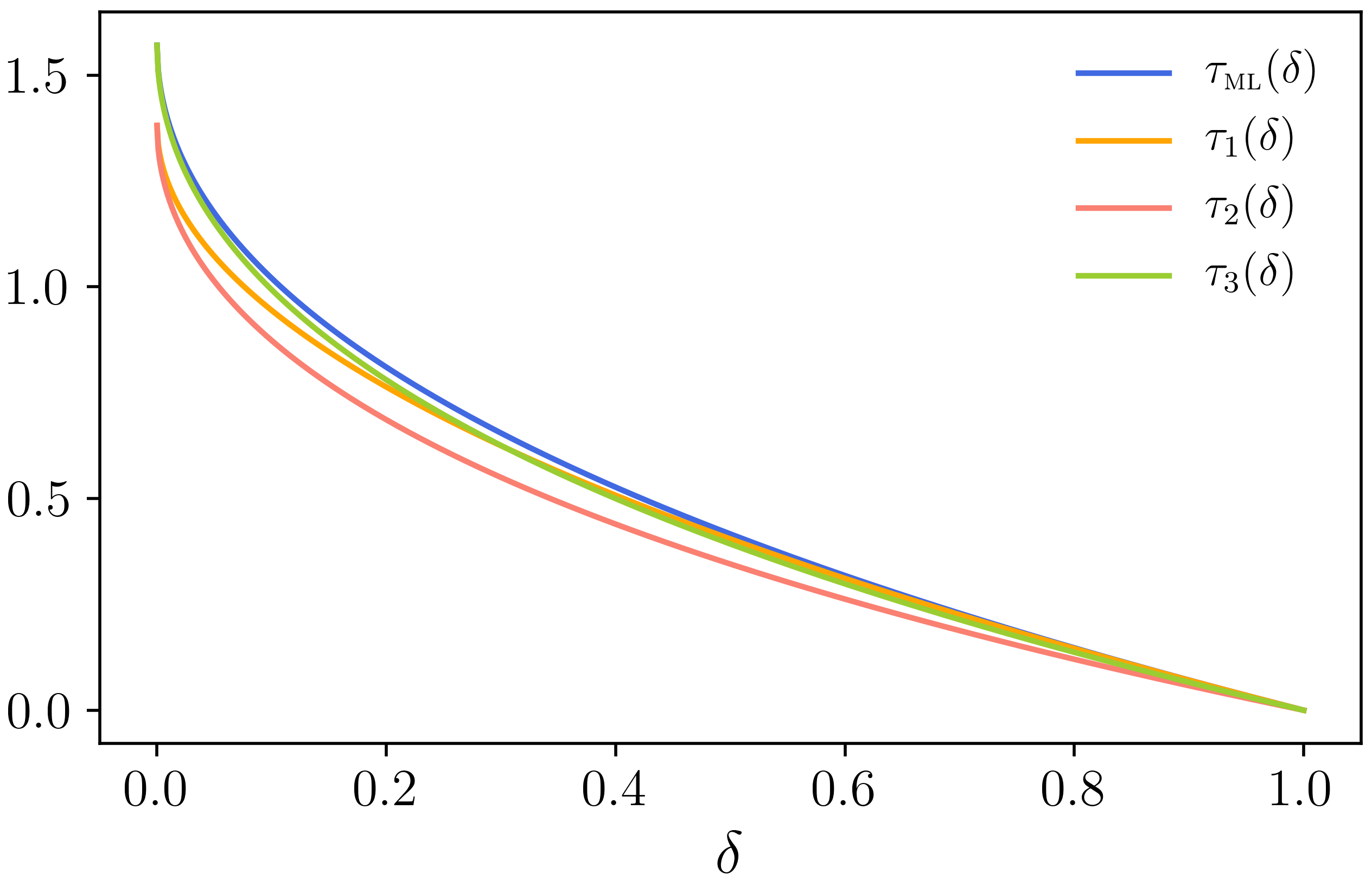
Apparently, , , and are weaker than , and is weaker than and . However, which of and is the stronger QSL depends on the fidelity , with being greater than for large values of and being greater than for small values of .
V Summary and outlook
Giovannetti et al. [10] showed, partly numerically, that if an isolated system evolves between two states with fidelity , then the evolution time is bounded from below by the extended Margolus-Levitin QSL (4). Giovannetti et al. also showed that this QSL is tight in all dimensions.
In this paper, we have derived the extended Margolus-Levitin QSL analytically and characterized the systems for which this QSL is saturated. Furthermore, we have interpreted the extended Margolus-Levitin QSL geometrically as an extremal dynamical phase in a gauge specified by the system’s ground state. We have also shown that the maximum of the Mandelstam-Tamm and the extended Margolus-Levitin QSLs is a tight QSL that behaves differently depending on whether or not the initial state and the final state are fully distinguishable. In addition, we have derived a tight dual version of the extended Margolus-Levitin QSL using a straightforward time-reversal argument. The dual QSL has similar properties as the extended Margolus-Levitin QSL and saturates under similar circumstances but involves the largest rather than the smallest occupied energy. We showed that the two QSLs can only be saturated simultaneously if the start and end states are fully distinguishable. We concluded the paper by reproducing three QSLs related to, but slightly weaker than, the extended Margolus-Levitin QSL.
A recent paper on evolution time estimates for closed systems [14] suggests that the Margolus-Levitin QSL does not straightforwardly extend to systems whose dynamics are governed by time-dependent Hamiltonians, at least not without limitations on the width of the energy spectrum.
The geometric analysis performed here shows that extended Margolus-Levitin QSL is closely related to the Aharonov-Anandan geometric phase [13]. This observation is further elaborated in Ref. [19] where QSLs for cyclically evolving systems are derived.
Mixed state QSLs resembling the Margolus-Levitin QSL exist [24, 23, 22], and Giovannetti et al. [10] showed that also the extended Margolus-Levitin QSL can be generalized to a QSL for systems in mixed states, with being the Uhlmann fidelity between the initial and final states [25]. Whether this generalization has a symplectic-geometric interpretation similar to the one presented here is an open question. So is the question whether the generalized extended Margolus-Levitin QSL connects to a geometric phase for mixed states [23, 28, 29, 27, 26]. The authors intend to investigate these questions in a forthcoming paper.
Acknowledgments
We thank Dan Allan for valuable discussions.
Appendix A The extended Margolus-Levitin quantum speed limit for qubit systems
Let be the Hamiltonian in (6) and be a qubit state whose Bloch vector is defined by (7)–(9). Then
| (49) |
Equation (10) follows from
| (50) |
To prove equation (11) consider two qubit states and with Bloch vectors and , respectively. Let be the fidelity between and . Then
| (51) |
This proves equation (11).
The dynamics caused by can be described as a rigid rotation of the Bloch sphere about the axis. To prove (12) assume and that rotates to during the evolution. Since the coordinate remains fixed, follows a path of the same length as the orthogonal projection of on the plane. The projection rotates to the projection of along a circular arc in the plane. The radius of the corresponding circle sector is
| (52) |
Furthermore, according to (11), the circle sector has apex angle
| (53) |
Thus, the length of the circular arc is
| (54) |
Finally, to prove (13) we first determine the speed of the rotating Bloch vector. Write , , and for the coordinates of the rotating Bloch vector. We have
| (55) |
Hence and . The rotating Bloch vector thus has the speed
| (56) |
This equation also says that causes the Bloch sphere to rotate with the angular speed about the axis. The evolution time equals the distance traveled by the Bloch vector divided by the speed of the Bloch vector,
| (57) |
This is the statement in equation (13).
Appendix B Characterization of time-optimal systems
Consider a quantum system of dimension . Let and set
| (58) |
where the infimum is over all triples consisting of a Hamiltonian , a state , and a time such that
| (59) |
As before, is the smallest eigenvalue of . In this appendix we show that some triple realizes the infimum and that for any such triple, is a partly grounded effective qubit for . Furthermore, we show that is the same for all and thus equals defined in equation (5). Note that condition (59) says that if controls the dynamics of the system, then will evolve to a state with fidelity in time .
B.1 Reduction to admissible pairs
We begin by establishing that
| (60) |
where the infimum is over all pairs consisting of a Hamiltonian with spectrum in and a state such that
| (61) |
We call such a pair admissible.
Take an arbitrary triple that satisfies condition (59). Let and set . The Hamiltonian is positive, has the minimum eigenvalue , and gives rise to dynamics identical to that caused by . Hence, satisfies condition (59). Since and have the same eigenspaces and, in particular, they have the same eigenspace for their smallest eigenvalues, is a partly grounded effective qubit for if and only if is a partly grounded effective qubit for .
Next, we normalize the evolution time by setting . The Hamiltonian is positive, has the minimum eigenvalue , and evolves to along the same path as but in time . Thus satisfies condition (59). Since and have the same eigenspaces, especially for the eigenvalue , is a partly grounded effective qubit for if and only if is a partly grounded effective qubit for .
Lastly, we define as the Hamiltonian obtained from by replacing each eigenvalue of with the in satisfying . The Hamiltonian is positive, has the smallest eigenvalue , and evolves to in time . The expectation value of is not greater than that of . We thus have that
| (62) |
This shows that , where the infimum is over all admissible pairs. The reverse inequality is automatically satisfied. Since the space of admissible pairs is compact, is attained for an admissible pair.
Now, suppose that is a partly grounded effective qubit for and thus for . Then is also a partly grounded effective qubit for . For eigenspaces of can merge when forming , but not in such a way that the support of is covered by the eigenspace of that belongs to the eigenvalue . The reverse, however, is not necessarily true. If is a partly grounded effective qubit for , need not be a partly grounded effective qubit for . But in that case, the inequality in (62) is strict, and the original triple does not saturate (58).
Remark 8.
One can choose the state arbitrarily and further restrict the infimum to Hamiltonians that form an admissible pair with the selected state. For if satisfies (59), is an arbitrary state, is a unitary such that , and , then also satisfies (59). Furthermore, and have the same spectrum, the expectation value of when the state is is the same as the expectation value of when the state is , and is a partly grounded effective qubit for if and only if is a partly grounded effective qubit for .
B.2 Not fully distinguishable initial and final states
Assume that . (For the sake of completeness, we treat the case in Appendix B.3, although this case has been dealt with earlier [15, 16].) Let denote a point in the compact rectangular block . Define the functions , , and on as
| (63) | |||
| (64) | |||
| (65) |
Furthermore, let be the subset of defined by the constraints and . Since is compact and is continuous, the restriction of to , denoted , assumes a minimum value. This minimum value is . To see this suppose that is an admissible pair such that . Let be the eigenvalues of , with corresponding eigenvectors , and set . The point belongs to , since and , and . Thus, assumes the value . To see that is the smallest value of let is an arbitrary point in . Then, let be an arbitrary orthonormal basis for the Hilbert space of the system and define and . The pair is admissible and . Hence, .
Let be a point in at which assumes its minimum value and let be the set of indices for which . The minimum point has the following properties:
-
(i)
There are indices and in such that and .
-
(ii)
For all indices and in such that and we have that .
Before showing that has these properties let us discuss their implications for the extended Margolus-Levitin QSL.
Assume that is an admissible pair such that . Let be the spectrum of and let be the probability of obtaining when measuring in the state divided by the degeneracy of . The point belongs to since according to the normed evolution time condition (61) and according to the law of total probability. Furthermore, assumes its minimum value at since . Property (i) says that is partly grounded; that is, its support is not orthogonal to the eigenspace belonging to the smallest eigenvalue of , which in this case is . Property (ii) says that is an effective qubit because the support of is only non-orthogonal to one eigenspace other than that belonging to .
Let us now prove properties (i) and (ii). For clarity let denote an arbitrary, unspecified point in and let be a point in at which assumes its minimum value. Let be the number of nonzero s. Since the values of , , and are invariant under rearrangements of the form , where is a permutation of the set , we can assume that the nonzero s are placed first in the sequence , so that , where is the vector consisting of zeros, and that the corresponding s are arranged in descending order of magnitude. We assume that the number of nonzero s among the first is . These constitute the first elements of . We denote the remaining s by , so that . The minimum point has the following properties:
-
(a)
are strictly less than . For suppose that some . If we change the value of this to , and will not change their values, and hence we are still in . However, since , such a change lowers the value of . This contradicts that assumes its minimum value at .
-
(b)
There exists a such that and , and thus . For suppose that . The functions and assume the same values at and , so both points belong to . However, since , has a lower value at the latter point. This contradicts that assumes its minimum value in . Since not all the s can be zero, statement (i) follows.
It remains to prove statement (ii), that is, that all the nonzero have the same value. Since we have assumed that , there exists a unique function on with values in the interval such that
| (66) | |||
| (67) |
This follows immediately from the observation that if and only if for a unique in . Now, consider the restrictions of , , and to :
| (68) | |||
| (69) | |||
| (70) |
The point lies in the intersection of and the interior of . Let . The gradient vectors of , , and at are
| (71) | ||||
| (72) | ||||
| (73) |
None of these are zero. According to the method of Lagrange multipliers, there are real and nonzero constants and such that . We thus have that
| (74) | ||||
| (75) | ||||
| (76) |
Equations (74) and (75) hold for . These equations imply that all the s are solutions to the quadratic equation . For if we move to the left side in (74), square both (74) and (75), and then add them, we obtain the equation . Thus, the s can assume at most two values,
| (77) | |||
| (78) |
We assume that both of these are present among the s. (Otherwise, we are done.) According to (77) and (78), is the arithmetic mean of and . Furthermore, (74) and (75) imply that
| (79) | ||||
| (80) |
Thus,
| (81) |
for an odd integer . Consequently,
| (82) | |||
| (83) |
Together with (74) och (75), these equations imply
| (84) |
Since and has the unique solution in this interval, we can conclude that .
B.3 Fully distinguishable initial and final states
If we must modify the previous section’s arguments slightly. We start by replacing with the two functions
| (85) | |||
| (86) |
and define as the subset of given by the constraints , , and . We again let be a point in at which assumes its minimum value, which in this case is . We arrange the coordinates in as in Appendix B.2. Properties (a) and (b) of also apply in this case. We consider the restrictions of , , , and to :
| (87) | |||
| (88) | |||
| (89) | |||
| (90) |
The point lies in the intersection of and the interior of , and the gradient vectors of the restrictions of , , and to at are
| (91) | ||||
| (92) | ||||
| (93) | ||||
| (94) |
None of these are zero. According to the method of Lagrange multipliers there exist real nonzero constants , , and such that . We thus have that
| (95) | ||||
| (96) | ||||
| (97) |
Equations (95) and (96) hold for . If we move to the left side in (95), square both (95) and (96), and then add them, we get the equation . Thus there are only two possibilities for the s,
| (98) | |||
| (99) |
We assume both are present among the s and, therefore, are strictly positive. The multiplier , and hence , is the arithmetic mean of and . It follows that
| (100) |
This equation cannot be satisfied for positive and . Thus, we have reached a contradiction. The conclusion is that only one of and is present among the s and, therefore, all the s have the same value.
B.4 Conclusion
Appendices B.2 and B.3 show that if assumes its smallest possible value under the requirement that the state evolves between two states with fidelity , then the state is a partly grounded effective qubit. Consequently, the case reduces to that treated in Sec. II.1, regardless of the dimension of the system. We conclude that and thus that the extended Margolus-Levitin QSL (4) is valid in all dimensions.
Appendix C Geodesics and ruled Seifert surfaces
A curve in is a geodesic if its acceleration vanishes, . For the Fubini-Study metric, ; see, e.g., Ref. [8]. Let and be two states at a distance apart. There is a unique shortest unit speed geodesic from to : Choose a unit vector over and let be the unit vector over that is in phase with . Then . Define by the condition , and let . The curve
| (101) |
is the shortest unit speed geodesic that extends from to ; straightforward calculations show that , that , and that has the length .
C.1 Optimal evolution curves are sub-Riemannian geodesics
If the extended Margolus-Levitin QSL is saturated, the state is a partly grounded effective qubit:
| (102) |
Here and are eigenvectors of the Hamiltonian with eigenvalues and , respectively. This state evolves on the geodesic sphere around with radius . The evolution curve is
| (103) |
This curve has the acceleration
| (104) |
The acceleration vanishes identically if and only if . In this case, the state moves along the equator in the projectivization of the span of and . Otherwise, the evolution curve is not a geodesic in . However, since the acceleration is everywhere perpendicular to , the evolution curve is a sub-Riemannian geodesic in , that is, a geodesic when considered a curve in with the sub-Riemannian geometry. To see this, fix a and let , , be the shortest, arclength-parametrized geodesic from to . According to Gauss’s lemma [30], its velocity vector at is perpendicular to . Explicitly, we have that
| (105) |
By equations (104) and (105), , which implies that is perpendicular to at . Consequently, is a sub-Riemannian geodesic.
C.2 Ruled Seifert surfaces
Let , , be a curve in which for each is at the distance from . We can construct a Seifert surface for its closure in the following way. Let be a lift of , let be the lift of that is in phase with , define by the condition , and set for and . Then is a Seifert surface for consisting of geodesics starting from and ending at points on .
Appendix D Extreme values of
Let be an arbitrary state and be the set of smooth curves in that stretches between two states with fidelity . Consider the functional on defined as
| (106) |
We calculate the extreme values of .
Fix an arbitrary lift of and recall that is the hypersurface in consisting of all vectors in phase with . Let be the first vector in an orthonormal basis for . Every lift of a curve in to has a decomposition of the form , where
| (107) |
for some real-valued functions and satisfying
| (108) |
Conversely, any such curve in projects to a curve in . Let and assume that . Then
| (109) |
Suppose that the fidelity between and is and that is extremal for . The s and s then satisfy the Euler-Lagrange equations for the augmented Lagrangian
| (110) |
The Euler-Lagrange equations read
| (111) | |||
| (112) | |||
| (113) |
These equations imply that , with being the integral of the Lagrange multiplier,
| (114) |
Thus, . That the fidelity between and is translates to
| (115) |
We conclude that
| (116) |
and, hence, that
| (117) |
References
- [1] M. R. Frey, Quantum speed limits—primer, perspectives, and potential future directions, Quantum Inf. Process. 15, 3919 (2016).
- [2] S. Deffner and S. Campbell, Quantum speed limits: From Heisenberg’s uncertainty principle to optimal quantum control, J. Phys. A: Math. Theor. 50, 453001 (2017).
- [3] S. Deffner, Quantum speed limits and the maximal rate of information production, Phys. Rev. Res. 2, 013161 (2020)
- [4] D. P. Pires, M. Cianciaruso, L. C. Céleri, G. Adesso, and D. O. Soares-Pinto, Generalized geometric quantum speed limits, Phys. Rev. X 6, 021031 (2016)
- [5] A. del Campo, I. L. Egusquiza, M. B. Plenio, and S. F. Huelga, Quantum speed limits in open system dynamics, Phys. Rev. Lett. 110, 050403 (2013).
- [6] L. Mandelstam and I. Tamm, The uncertainty relation between energy and time in non-relativistic quantum mechanics, J. Phys. (USSR) 9, 249 (1945).
- [7] J. Anandan and Y. Aharonov, Geometry of quantum evolution, Phys. Rev. Lett. 65, 1697 (1990).
- [8] N. Hörnedal, D. Allan, and O. Sönnerborn, Extensions of the Mandelstam–Tamm quantum speed limit to systems in mixed states, New J. Phys. 24, 055004 (2022).
- [9] N. Margolus and L. B. Levitin, The maximum speed of dynamical evolution, Phys. D 120, 188 (1998).
- [10] V. Giovannetti, S. Lloyd, and L. Maccone, Quantum limits to dynamical evolution, Phys. Rev. A 67, 052109 (2003).
- [11] M. M. Taddei, B. M. Escher, L. Davidovich, and R. L. de Matos Filho, Quantum speed limit for physical processes, Phys. Rev. Lett. 110, 050402 (2013).
- [12] M. M. Taddei, Quantum Speed Limits for General Physical Processes, Ph.D. thesis, Universidade Federal do Rio de Janeiro, 2014 (unpublished), arXiv:1407.4343.
- [13] Y. Aharonov and J. Anandan, Phase change during a cyclic quantum evolution, Phys. Rev. Lett. 58, 1593 (1987)
- [14] N. Hörnedal and O. Sönnerborn, Closed systems refuting quantum-speed-limit hypotheses, Phys. Rev. A 108, 052421 (2023).
- [15] J. Söderholm, G. Björk, T. Tsegaye, and A. Trifonov, States that minimize the evolution time to become an orthogonal state, Phys. Rev. A 59, 1788 (1999).
- [16] L. B. Levitin and T. Toffoli, Fundamental limit on the rate of quantum dynamics: The unified bound is tight, Phys. Rev. Lett. 103, 160502 (2009).
- [17] N. Mukunda and R. Simon, Quantum kinematic approach to the geometric phase. I. General formalism, Ann. Phys. 228, 205 (1993).
- [18] G. E. Bredon, Topology and Geometry, Graduate Texts in Mathematics (Springer, New York, 1993).
- [19] N. Hörnedal and O. Sönnerborn, Tight lower bounds on the time it takes to generate a geometric phase, Phys. Scr. 98, 105108 (2023).
- [20] G. Ness, A. Alberti, and Y. Sagi, Quantum speed limit for states with a bounded energy spectrum, Phys. Rev. Lett. 129, 140403 (2022).
- [21] D. C. Brody, Elementary derivation for passage times, J. Phys. A: Math. Gen. 36, 5587 (2003).
- [22] O. Andersson and H. Heydari, Quantum speed limits and optimal Hamiltonians for driven systems in mixed states, J. Phys. A: Math. Theor. 47, 215301 (2014).
- [23] O. Andersson, Holonomy in Quantum Information Geometry, Ph. Lic. thesis, Stockholm University, 2018 (unpublished), arXiv:1910.08140.
- [24] M. Andrecut and M. K. Ali, The adiabatic analogue of the Margolus–Levitin theorem, J. Phys. A: Math. Gen. 37, L157 (2004).
- [25] A. Uhlmann, The “transition probability” in the state space of a -algebra, Rep. Math. Phys. 9, 273 (1976).
- [26] A. Uhlmann, Geometric phases and related structures, Rep. Math. Phys. 36, 461 (1995).
- [27] E. Sjöqvist, A. K. Pati, A. Ekert, J. S. Anandan, M. Ericsson, D. K. L. Oi, and V. Vedral, Geometric phases for mixed states in interferometry, Phys. Rev. Lett. 85, 2845 (2000)
- [28] O. Andersson and H. Heydari, A symmetry approach to geometric phase for quantum ensembles, J. Phys. A: Math. Theor. 48, 485302 (2015).
- [29] A. Uhlmann, Operational geometric phase for mixed quantum states, New J. Phys. 15, 053006 (2013).
- [30] T. Sakai, Riemannian Geometry, Translations of Mathematical Monographs (American Mathematical Society, Providence, Rhode Island, 1996), Vol. 149.