Planar Object Tracking via Weighted Optical Flow

Abstract

We propose WOFT – a novel method for planar object tracking that estimates a full 8 degrees-of-freedom pose, i.e. the homography w.r.t. a reference view. The method uses a novel module that leverages dense optical flow and assigns a weight to each optical flow correspondence, estimating a homography by weighted least squares in a fully differentiable manner. The trained module assigns zero weights to incorrect correspondences (outliers) in most cases, making the method robust and eliminating the need of the typically used non-differentiable robust estimators like RANSAC. The proposed weighted optical flow tracker (WOFT) achieves state-of-the-art performance on two benchmarks, POT-210 [23] and POIC [7], tracking consistently well across a wide range of scenarios.

1 Introduction

In this paper, we address the rigid planar object tracking problem, which is a specific subtopic of visual object tracking. Given an object identified in the first frame, a tracker should output the tracked object pose or absence of the object in the frame, on every subsequent frame of a video sequence. In a general model-free setting, the tracker has no prior knowledge about the target class except for target-specific information coming from the first frame initialization. In standard tracking benchmarks, such as OTB [46], VOT [18, 20], LaSOT [11], TrackingNet [30], or YT-BB [36], the object pose is represented by axis-aligned or rotated bounding boxes. Tracking with segmentation mask representation has gained popularity in recent years, with benchmarks such as VOT2020 [19], DAVIS [33, 35], and YouTube-VOS [47].

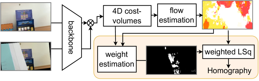
Figure 1: Planar object tracking with a homography estimated by a novel weighted least squares (LSq) homography module called WFH (orange box) on optical flow correspondences. The proposed trainable flow weight CNN assigns a weight $w_{i}\in[0,1]$ to each flow vector based on samples from correlation cost-volume.

In planar rigid object tracking, the object pose is related to its initial pose by an 8 degrees-of-freedom (DoF) homography when using a perspective camera, and the target is fully specified by the initialization mask. Planar trackers can output precise 8-DoF object poses, enabling applications not possible with bounding-box or segmentation mask level trackers, in areas such as film post-production, visual servoing [50, 5], SLAM [41], or markerless augmented reality [44, 34, 39]. Man-made objects are often either completely planar or consist of planar surfaces, allowing for planar object tracking in a wide range of scenarios.

Current state-of-the-art methods struggle on seemingly toy-like sequences in standard planar object tracking datasets, POT-210 [23] and POIC [7]. The target planarity poses challenges, e.g., strong perspective distortion, significant illumination changes caused by specular highlights, and motion blur caused by a shaking hand-held camera.

In this work, we introduce a novel model-free planar object tracker. The proposed method estimates dense correspondences between the template (initial image) and the current image with a deep optical flow network. A novel homography estimation module then assigns a weight to each optical flow correspondence, and a homography is estimated as a solution to a weighted least squares problem. The network assigns low weights to incorrect flow vectors and thus it is not necessary to use robust outlier detection algorithms like RANSAC.

Using dense OF correspondences has several advantages. First, OF estimation is well researched and high-quality methods are available off-the-shelf. Second, the dense per-pixel correspondences help on low-textured objects, where sparse key-point correspondences fail. Finally, having dense correspondences enables us to compute a homography correspondence support set and detect a tracking failure if the support is small.

The proposed homography estimation procedure is fully differentiable, allowing us to train both the weight estimator and the optical flow network using homography supervision. The main contributions of this work are the following.

• We propose a novel fully differentiable homography estimation neural network module.

• We propose a novel planar target tracker employing the weighted flow homography estimation (code public).

• The proposed tracker sets a new state-of-the-art on the POT-210 [23], POT-280 [22], and POIC [23] datasets, performing well across all challenge types. On POT-210, the tracker error is half of the error of the best competing method.

• We analyze the ground truth on the POT-210 dataset and publish a precise re-annotation of its subset. The inaccuracy of the original annotation accounted for half of the errors of the proposed tracker.

2 Related Work

General visual object tracking methods have been improving consistently, with deep-learning-based trackers dominating classical methods[21, 19]. In contrast, planar object trackers have only recently started using deep learning.

The homography trackers can be roughly divided into three main categories [23]: keypoint methods, direct methods, and deep methods. Traditional keypoint-based tracking consists of three steps: (i) keypoint detection and description using, e.g., SIFT[27] or SURF[3], (ii) keypoint matching by nearest neighbor search in the descriptor space, and (iii) robust homography estimation with RANSAC [12]. The SOL [14] tracker uses SVM to learn keypoint descriptors and PROSAC [9] ordering. In Gracker [45], the keypoints are not matched independently based only on descriptor similarity, but instead a graph-matching approach is used. The OBD [29] tracker uses ORB keypoints for target detection and optical flow tracking. In the POT-280 [22] benchmark, the authors compare several deep-learning based homography trackers. The best ones use the SIFT keypoint detector, a deep learning descriptor such as GIFT [25], MatchNet [13], SOSNet [43], or LISRD [32], followed by RANSAC.

Direct methods formulate the tracking task as image registration. Given the current frame, they attempt to find a homography warping that optimizes the alignment of the current frame with the object in the initial frame. In the classical Lucas-Kanade [28] and the Inverse Compositional [2] methods, the warp quality is measured directly on the image intensities by a sum of squared differences. The ESM [4] tracker avoids the costly computation of Hessian in Lucas-Kanade by using an efficient second-order minimization (ESM) technique. GO-ESM [8] improved robustness to illumination changes by adding a gradient orientation feature on top of the image intensities and generalizing the ESM tracker to multidimensional features. The GOP-ESM [7] tracker extends GO-ESM with a feature pyramid and a coarse-to-fine iterative approach. Chen et al. [6] proposed to use the ESM algorithm as a differentiable layer in a siamese neural network architecture. The ESM layer iteratively aligns the template and the query frame feature maps obtained from a ResNet-18 [16] backbone pre-trained on ImageNet. The whole architecture is then fine-tuned on image pairs synthesized from the MS-COCO dataset [24]. Direct methods perform well on the POIC[7] dataset, but typically fail on motion blur, partial occlusions and partially out-of-view targets, e.g. in the POT-210 [23] dataset.

Deep learning homography estimation is typically done by regression of four control points. The HomographyNet [10] and UDH [31] feed a concatenated pair of homography-related images through a CNN and formulate the homography estimation as direct regression of four control points. Rocco et al. [37] proposed to regress the four homography control points from a correlation cost-volume containing each-to-each similarities between Siamese VGG-16 [40] feature maps. The four-point regression is also used by the recently proposed HDN [49] method, which decomposes the homography into a similarity transform and a homography residual. These control-point regression methods struggle with occlusions and often assume that the whole images are related by a homography, and do not distinguish between the target and the background motion. The PFNet [48] uses a custom convolutional architecture to estimate a dense flow field, which is then used in RANSAC, making the method not differentiable and end-to-end training not possible.

3 Method

We propose a weighted flow homography module (WFH) that assigns a flow weight $w_{i}\in[0,1]$ to each OF correspondence and estimates a homography using a weighted least squares formulation (Sec. 3.1). The WFH is differentiable, making end-to-end training of both the WFH and the OF network possible. In Sec. 3.2, we propose a weighted optical flow tracker (WOFT) built around the WFH homography estimator.

3.1 Weighted Flow Homography Module

The idea of the WFH module is to compute a flow weight $w_{i}\in[0,1]$ for each optical flow vector and to predict a homography by solving a weighted least squares (LSq) problem. The standard least squares homography fitting is sensitive to grossly incorrect correspondences (outliers). This is usually addressed by RANSAC, which uses repeated hypothesis sampling to find a homography and its outlier-free correspondence support set. The WFH instead eliminates outliers by setting their flow weights close to zero, allowing for a robust, single iteration, and fully differentiable weighted least squares fitting.

We process a pair of images with an optical flow estimation network, such as RAFT [42] to get OF correspondences $\left({\mathbf{p}}_{i},{\mathbf{p^{\prime}}}_{i}\right)$, where ${\mathbf{p}}_{i}=(x_{i},y_{i})$ is a position in one image and ${\mathbf{p}}_{i}^{\prime}=(x_{i}^{\prime},y_{i}^{\prime})$ the corresponding position in the second image. We then pass a suitable inner representation of the OF network to a weight-estimation CNN that predicts the flow weight $w_{i}$ for each OF vector. Finally, we estimate homography by solving a system of equations by weighted least squares. First, we introduce plain least squares homography estimation, then we describe the weighted variant and the training loss function. Finally, we describe the weight estimation CNN in detail.
LSq Homography. Given the optical flow correspondences, we want to find a homography matrix ${\mathbf{H}}\in\mathbb{R}^{3\times 3}$ mapping $\left(x_{i},y_{i},1\right)$ to $\left(\lambda x_{i}^{\prime},\lambda y_{i}^{\prime},\lambda\right)$, $\lambda\neq 0$. This leads to an overdetermined homogeneous system of equations ${\mathbf{A}}{\mathbf{h}}={\mathbf{0}}$, with ${\mathbf{h}}\in\mathbb{R}^{9\times 1}$ being the flattened ${\mathbf{H}}$-matrix and ${\mathbf{A}}\in\mathbb{R}^{2N\times 9}$ encoding the data constraints. The system is usually solved in the least-norm sense via a singular value decomposition (SVD) of ${\mathbf{A}}$. We use the PyTorch machine learning framework which includes differentiable SVD, but the back-propagated gradients are often unstable. To overcome this issue, we constrain the homography by fixing its bottom-right element $h_{3,3}=1$, leading to a non-homogeneous system $\tilde{{\mathbf{A}}}\tilde{{\mathbf{h}}}={\mathbf{b}}$, which can be solved in the least-squares sense using the QR decomposition with more stable gradients. Not all homographies are representable with this constraint (see Sec. 4.1.2 in [15]), but we have not encountered such a case in the tracking scenario.

In the non-homogeneous formulation, each correspondence adds two equations into $\tilde{{\mathbf{A}}}\in\mathbb{R}^{2N\times 8}$ and ${\mathbf{b}}\in\mathbb{R}^{2N}$:

$$\begin{bmatrix}0&0&0&-x_{i}&-y_{i}&-1&y_{i}^{\prime}x_{i}&y_{i}^{\prime}y_{i}\\ x_{i}&y_{i}&1&0&0&0&-x_{i}^{\prime}x_{i}&-x_{i}^{\prime}y_{i}\\ \end{bmatrix}\tilde{{\mathbf{h}}}=\begin{bmatrix}-y_{i}^{\prime}\\ x_{i}^{\prime}\end{bmatrix}$$ (1)

Figure 2: High weights of optic flow (yellow) appear mainly on corners and well-textured areas. Bottom: the POT-210 target with the highest average flow weights (left); weight values drop (purple) when ”occluded” by a reflection (right). Best viewed in color.

We solve the least squares problem

$$\min\limits_{\tilde{{\mathbf{h}}}}\sum\limits_{j=1}^{2N}\lVert\tilde{{\mathbf{A}}}_{j,\cdot}\tilde{{\mathbf{h}}}-{\mathbf{b}}_{j}\rVert_{2}^{2}$$ (2)

by QR decomposition of the data matrix $\tilde{{\mathbf{A}}}={\mathbf{Q}}{\mathbf{R}}$ followed by solving the triangular system ${\mathbf{R}}\tilde{{\mathbf{h}}}={\mathbf{Q}}^{\intercal}{\mathbf{b}}$ (triangular system solver available in PyTorch).
Weighted LSq Homography. In the proposed weighted least squares formulation, we weight each pair of equations with the corresponding estimated flow weight $w_{i}$ and find

$$\min\limits_{\tilde{{\mathbf{h}}}}\sum\limits_{j=1}^{2N}w_{j}\lVert\tilde{{\mathbf{A}}}_{j,\cdot}\tilde{{\mathbf{h}}}-{\mathbf{b}}_{j}\rVert_{2}^{2}$$ (3)

$$=\min\limits_{\tilde{{\mathbf{h}}}}\sum\limits_{j=1}^{2N}\lVert\left(\sqrt{w_{j}}\tilde{{\mathbf{A}}}\right)_{j,\cdot}\tilde{{\mathbf{h}}}-\left(\sqrt{w_{j}}{\mathbf{b}}_{j}\right)\rVert_{2}^{2}$$ (4)

The weighted problem (3) is transformed into non-weighted (Eq. (2)) by multiplying each row of $\tilde{{\mathbf{A}}}$ and each element of ${\mathbf{b}}$ by the square root of the corresponding weight $\sqrt{w_{i}}$.
Training WFH. We train the WFH weight estimation CNN using a loss function on the predicted homography. We warp points forward by the ground truth homography ${\mathbf{H}}_{GT}$ then backward by the inverse of the estimated ${\mathbf{H}}$ and finally compute L1 loss on the projection errors as:

$$L({\mathbf{H}})=\frac{1}{N}\sum\limits_{i=1}^{N}\lVert p_{i}-{\mathbf{H}}^{-1}{\mathbf{H}}_{GT}p_{i}\rVert_{2}$$ (5)

Both the optical flow network and the flow weight estimation CNN are trained using a single loss function, and we do not use additional direct supervision of the flow weight predictor. The learned flow weights resemble a keypoint detector output (corners, well-textured patches), but with information from both images, therefore giving low weights on occlusions or significant appearance changes as shown in figure 2.
Weight Estimation CNN The proposed WFH module operates on the correlation cost-volume pyramid of the RAFT [42] optical flow estimator, but the idea is applicable to other OF networks (Sec. 4.2). RAFT computes a correlation volume $\mathbf{C}^{1}\in\mathbb{R}^{H/8\times W/8\times H/8\times W/8}$ that captures the similarity between all pairs of feature vectors extracted from the two input images. Next, they construct a 4-layer correlation pyramid $\left\{\mathbf{C}^{1},\mathbf{C}^{2},\mathbf{C}^{3},\mathbf{C}^{4}\right\}$. Finally, $9\times 9$ patches centered on current flow vector estimates are sampled from this pyramid and processed by a neural network that produces a flow vector update. This is repeated several times to produce the final optical flow field.

In WFH we sample the correlation pyramid once more on the final OF positions, resulting in a $9\times 9\times 4$ feature map for each flow vector in the spatial resolution of $H/8\times W/8$. To capture the global context, we then append an additional channel containing the mean correlation volume response $M(i,j)=\sum\limits_{m=1}^{H/8}\sum\limits_{n=1}^{W/8}\mathbf{C}_{i,j,k,l}^{1}$ for the given position $(i,j)\in\{1,\dots,H/8\}\times\{1,\dots,W/8\}$ in the first input image feature map. We process the resulting features $f_{i,j}\in\mathbb{R}^{9\times 9\times 5}$ with a three-layer convolutional network (kernel size 3, 128 output channels, ReLU) followed by a $1\times 1$ convolution (single output channel) and global average pooling. Finally, we up-sample the results with the RAFT up-sampling module and apply a sigmoid activation to get a $H\times W$ score map with weights between $0$ and $1$.

3.2 Homography tracker

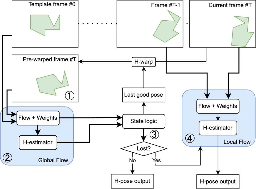
Figure 3: The WOFT tracker pre-warps the current frame using the last good pose (1). It then estimates a homography between the template and the pre-warped frame (2) and the reliability of the estimated homography is assessed (3). When the estimate is not reliable (‘lost‘ state) a homography based on a local flow (4) is returned instead.

We propose a planar object tracker based on the weighted flow homography module, WFH. Our weighted optical flow tracker, denoted WOFT, consists of four main parts as shown in Fig. 3.

First, we apply a pre-warping technique to reduce large pose differences, which are not handled well by OF methods. The current video frame $I_{t}$ is pre-warped by the homography from the last reliable frame $I_{G}$, with $G=0$ initially. The pre-warp $\tilde{I}_{t}=\mathcal{W}({\mathbf{H}}_{0\rightarrow G}^{-1},I_{t})$ reduces the pose difference between the template and the current images, resulting in a motion similar to the typical $I_{(t-1)}\rightarrow I_{t}$ optical flow scenario. The possible appearance difference between the template and a temporarily distant frame (caused mainly by illumination changes and motion blur) is implicitly handled by the optical flow feature encoder.

Second, we compute the global optical flow between the template frame $I_{0}$ and the pre-warped current frame $\tilde{I}_{t}$ and the corresponding flow weights. We mask the flow correspondences, only leaving the ones starting inside the template mask and ending inside the current image. To speed up the homography estimation, we randomly subsample the correspondences, only keeping 500. We then estimate homography ${\mathbf{H}}_{0\rightarrow\tilde{t}}$ using weighted least squares as described in Sec. 3.1. Computing the homography between the template and the pre-warped current frame prevents error accumulation and target drift (Sec. 4.2).

We pass the weighted optical flow together with the computed homography to a state logic block that decides whether the tracking was successful or not. The lost/not-lost decision is made based on the support set size of the estimated homography. In particular, with optical flow correspondences $({\mathbf{p}}_{i},{\mathbf{p}}_{i}^{\prime})$ we warp each position ${\mathbf{p}}_{i}=(x_{i},y_{i})$ using the homography ${\mathbf{H}}_{0\rightarrow\tilde{t}}$ and compute the Euclidean distance to the position ${\mathbf{p}}_{i}^{\prime}=(x_{i}^{\prime},y_{i}^{\prime})$. The $i$-th correspondence is an inlier when $\lVert\mathcal{W}({\mathbf{H}}_{0\rightarrow\tilde{t}},{\mathbf{p}}_{i})-{\mathbf{p}}_{i}^{\prime}\rVert\leq 5$ pixels – a standard threshold on planar tracking benchmarks [23, 7]. We declare the tracker lost when it has a small support set, i.e. less than $20\%$ inliers.

When the tracker is not lost, we return ${\mathbf{H}}_{0\rightarrow t}={\mathbf{H}}_{0\rightarrow G}^{-1}{\mathbf{H}}_{0\rightarrow\tilde{t}}$ and update the last good frame index used for pre-warping $G=t$. When the tracker is lost, we make a second attempt to estimate the pose using a local optical flow $I_{(t-1)}\rightarrow I_{t}$. The local flow tends to drift, but it helps to keep track of the target pose in the short term. The temporarily close input images are close in appearance (similar illumination, similar motion blur, etc.). We estimate ${\mathbf{H}}_{(t-1)\rightarrow t}$ by weighted least squares as described above and output ${\mathbf{H}}_{0\rightarrow t}={\mathbf{H}}_{(t-1)\rightarrow t}{\mathbf{H}}_{0\rightarrow(t-1)}$. Moreover, when the tracker is lost for more than 10 frames, we reset the pre-warping last good frame index $G=0$. The target pose can change significantly over the 10 frames, making the pre-warp information outdated. Moreover, a bad pre-warp homography can ruin any chance of recovering, e.g. an outdated strong perspective change pre-warp distorts the current target area beyond being recognizable, and the identity homography with $G=0$ is the safest choice.

3.3 Implementation details

For optical flow, we use the author-provided RAFT checkpoint trained on Sintel. We then train the weight estimation CNN for 10 epochs on a synthetic dataset with 50000 image pairs. We generate the training set by repeatedly sampling a random MS COCO[24] image and warping it with two random homographies representing the template and the current frame pose. The random homographies are generated by perturbing each corner of the image with a random vector of length up to $20\%$ of the image diagonal. We blur the second warped image by a random linear motion of length up to 20 pixels. Finally, both images are passed through JPEG compression with quality set to 25.

We train with AdamW [26] optimizer with an initial learning rate $1e^{-3}$, which is then halved after every epoch. Finally, we fine-tune the whole network, including RAFT for 2 epochs, starting from the learning rate $1e^{-5}$ and again halving it after every epoch. To stabilize the training procedure, we discard training samples achieving loss over 100.

The tracker runs at around 3.5 FPS on a GeForce RTX 2080 Ti GPU (i7-8700K CPU @ 3.70GHz). The majority of time is spent on the optical flow computation (275ms). The weight computation (2ms), the weight up-sampling (1ms), and the least squares homography estimation (5ms) take negligible time. Image pre-warping (done on CPU), optical flow masking, and subsampling cost an additional 7ms.

A faster variant WOFT_{$\downarrow\!s$} downscales the input images to $H/s\times W/s$ and rescales the output homographies to the original resolution.

Figure 4: Precise re-annotation examples. Original ground truth annotation (left), improved ground truth annotation (right). The grayscale template in green channel, the GT-warped current frame in red and blue channels. Imprecise annotation causes green and magenta shadows, while precisely aligned images produce a grayscale result. The green bands on top and on right side respectively are caused by a partial occlusion on current frame. The alignment error of the original GT evaluated on the improved ground truth is $15.8$px (top) and $7.2$px (bottom).

4 Experiments

We evaluate the proposed tracker on two standard planar object tracking datasets, POT-210 and POIC and show that it consistently achieves high accuracy and robustness.
POT-210[23]: The Planar Object Tracking in the Wild benchmark contains 210 videos of 30 objects. Each object appears in 7 video sequences with different challenging attributes – scale change, in-plane rotation, perspective distortion, motion blur, occlusion, out-of-view, and unconstrained. The sequences have a fixed length of 501 frames. POT-280 [22] extends POT-210 by 10 new objects.
POIC[7]: the Planar Objects with Illumination Changes dataset consists of 20 sequences of varying length giving a total of 22971 frames. The dataset contains sequences with translation, in- and out-of-plane rotations, and scale changes, but mainly focuses on strong specular highlights and other significant illumination changes, making it complementary to POT-210.
Evaluation protocol: On both POT-210 and POIC, a tracker is initialized on the first frame and left to track till the end of the sequence. The alignment error $e_{AL}$ is computed for each annotated frame. Given four reference points ${\mathbf{x}}_{i}\in X$ in the first frame, the alignment error is defined as root-mean-square error between their projection into the current frame by the ground truth homography ${\mathbf{H}}^{*}$ and by the tracker homography ${\mathbf{H}}$,

$$e_{AL}({\mathbf{H}};{\mathbf{H}}^{*},X)=\sqrt{\frac{1}{4}\sum\limits_{i=1}^{4}\left(\mathcal{W}({\mathbf{H}}^{*},{\mathbf{x}}_{i})-\mathcal{W}({\mathbf{H}},{\mathbf{x}}_{i}\right))^{2}},$$ (6)

with $\mathcal{W}({\mathbf{H}},{\mathbf{x}})$ representing the projection of vector ${\mathbf{x}}$ by a homography ${\mathbf{H}}$. Tracker precision is measured as a fraction of frames with $e_{AL}\leq 5$ px (P@5 score). Additionally, we measure $e_{AL}\leq 15$ px (P@15 score), corresponding to the fraction of frames with target not tracked perfectly, but not completely lost either – we call this robustness regime.

4.1 Ground truth quality

During the analysis of WOFT performance on POT-210, we found that in many cases the ground truth (GT) annotations are less accurate than the official 5px error threshold. We have performed reannotation of a subset of the POT-210 dataset to measure the original GT quality and provide more accurate estimates of tracker performance, see Fig. 4. Our annotation tool shows the template, the object on the current frame warped with the current annotation, and, most importantly, an alignment visualization. We convert both the template frame and the current frame to grayscale and overlay the warped frame over the template, putting the template into the green channel and the current frame into the red and the blue channels. This allows for very precise alignment over the whole extent of the target, unlike the annotation interface used for the original annotation (Fig. 4 in [23]). We have fully manually reannotated frames 82, 172, 252, 332, and 412 from each sequence, without seeing the WOFT estimated poses and the new GT will be made publicly available. More examples of the reannotation overlay are in the supplementary materials. The alignment error of the original GT evaluated on our re-annotation is $3.63$ on average, and worse than the official $5$px threshold in $15\%$ cases.

4.2 Ablation study

In Table 1, we show the impact of various design choices of WOFT on POT-210 performance (both on the original and the more accurate re-annotated ground truth). First, we show the importance of computing the optical flow between the template and the pre-warped current frame. In rows 1, 2 we only use the local flow (from $I_{(t-1)}$ to $I_{t}$). The tracker drifts and quickly loses the target, resulting in overall poor performance. A big performance improvement is achieved by using global flow (from $I_{0}$ to $\tilde{I}_{t}$) and always using the previous frame for pre-warping (rows 3, 4). Another boost in performance is achieved with the controlled pre-warping (rows 5 - 9), where the local flow is used when the global flow fails and the pre-warp homography is reset when the target is ‘lost‘ for more than 10 frames.

Using the weighted least squares homography estimation consistently improves the performance – compare row 2 to row 1 (P@5 $+1.3$), row 4 to row 3 (P@5 $+10.7$), and row 6 to row 5 (P@5 $+8.3$). In row 7, we used the same settings as in WOFT (row 6), but without the RAFT fine-tuning, resulting in a drop in P@5 ($-7.4$). We have also experimented (row 8) with estimating homography by weighted iterative reweighted least squares (IRLSq) instead of ordinary weighted least squares. We have set the IRLSq to optimize the Huber loss (also called smooth L1 loss) which is more robust to outliers than least squares. This did not change the performance (w.r.t. row 6), indicating that our estimated weights already take care of outliers and the robust estimator is not necessary. Next, we compare RANSAC (row 9) with the proposed WOFT (row 6). The weighted least squares approach achieves better results (P@5 $+0.9$) in a single differentiable pass.

Rows 10-12 show WOFT with LiteFlowNet2 [17] flow (details in supplementary) instead of RAFT. Again, the weighted LSq estimator (row 12) works better than plain LSq (row 10) or RANSAC (row 11).

						P@5		P@15
	M	PW	H	W	F	orig	rean	orig	rean
(1)	R	–	LSq	–	$\checkmark$	5.7	0.8	16.6	10.7
(2)	R	–	LSq	$\checkmark$	$\checkmark$	7.0	2.1	22.5	17.3
(3)	R	$\checkmark$	LSq	–	$\checkmark$	57.6	63.6	68.1	68.9
(4)	R	$\checkmark$	LSq	$\checkmark$	$\checkmark$	66.7	74.3	75.5	76.4
(5)	R	C	LSq	–	$\checkmark$	73.1	82.1	89.9	92.0
(6)	R	C	LSq	$\checkmark$	$\checkmark$	80.6	90.4	93.9	95.6
(7)	R	C	LSq	$\checkmark$	–	75.1	83.0	87.3	87.8
(8)	R	C	IRLSq	$\checkmark$	$\checkmark$	80.6	90.4	93.9	95.6
(9)	R	C	RSAC	–	$\checkmark$	79.5	88.8	92.7	93.5
(10)	L	C	LSq	–	–	66.9	74.8	82.3	82.6
(11)	L	C	RSAC	–	–	72.8	80.9	84.4	85.1
(12)	L	C	LSq	$\checkmark$	–	72.8	81.0	86.1	87.1

Table 1: Ablation study on POT-210, evaluated on the original ground truth (orig) and the reannotation (rean). In all experiments, weighted least squares perform better than non-weighted alternative in both P@5 and P@15. M – flow method: RAFT (R), LiteFlowNet2 (L). PW – use of the global pre-warped flow: never (–), always ($\checkmark$), controlled (C). H – homography estimation method: least squares (LSq), iterative re-weighted least squares with Huber loss (IRLSq), RANSAC (RSAC). W – using the estimated weights. F – using the fine-tuned RAFT flow.

4.3 Weights Evaluation

Figure 5 shows how the learned weights correlate with the optical flow quality. Low-textured areas and ambiguous features are often assigned a low weight (Fig. 2) even when the corresponding optical flow is correct. Importantly, the incorrect flow vectors are assigned low weights.

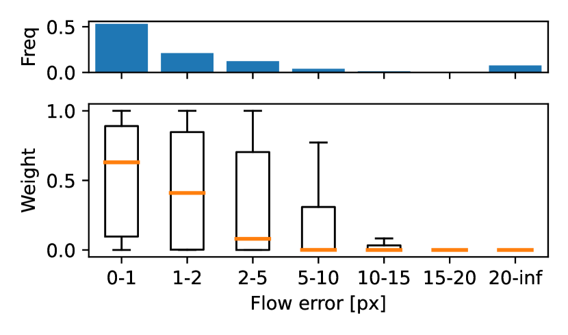
Figure 5: Weight distribution for different optical flow error ranges measured against the re-annotated POT-210 [23] ground truth. Median in orange. Top: frequency of each flow error range. The weight network learned to assign zero weight to incorrect flow vectors (outliers) and high weight to some correct flow vectors.

4.4 POT-210 and POT-280 evaluation

			P@5		P@15
method	year	FPS	orig	rean	orig	rean
GOP-ESM [7]	2019	4.95*	42.9	–	49.7	–
SuperGlue [38, 22]	2020	3.7*	39.1	42.1	58.0	55.7
Gracker [45]	2017	4.8*	39.2	–	63.2	–
SiamESM [6]	2019	–	58.7	–	66.2	–
SOSNet [43, 22]	2019	1.5*	56.6	60.9	69.9	67.0
SIFT [27, 22]	2004	0.8*	62.2	65.8	71.3	69.6
OBD [29]	2021	30*	48.4	54.3	79.3	79.2
LISRD [32, 22]	2020	7*	61.6	68.3	79.6	79.2
HDN [49]	2022	10.6*	61.3	70.9	91.5	92.4
WOFT$\downarrow$3 (ours)		19.2	68.9	80.5	91.2	92.3
WOFT (ours)		3.5	80.6	90.4	93.9	95.6

Table 2: Results on POT-210 [23] dataset. The proposed WOFT tracker sets a new state-of-the-art performance in both accuracy (P@5) and robustness (P@15). Evaluated on the original ground truth (orig) and the re-annotation (rean). Tracking speed in frames per second (FPS). ^* speeds from the papers, different hardware.

                        

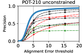
Figure 6: Alignment Error on POT-210 [23] (original GT). WOFT performs well on all sequence types, reducing the error on the official 5px threshold to half of the best competitor. Method types: (red circle) – keypoint, (green triangle) – direct, (black square) – deep.

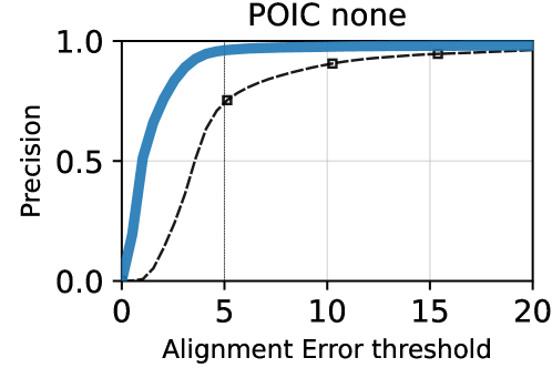
Figure 7: Alignment Error evaluation on POIC [7]. The proposed WOFT achieves state-of-the-art with $96.1$ P@5 and $98.0$ P@15.

We compare WOFT method against the best performing methods on the POT-210 [23] dataset. Namely keypoint methods: SIFT [27], OBD [29], and Gracker [45], deep control point regression HDN [49], the deep learning based methods evaluated in [22]: SOSNet [43], SuperGlue [38], LISRD [32], the direct methods: GOP-ESM [7], and Siam-ESM [6] (deep + direct).

The proposed WOFT achieves state-of-the-art on the POT-210 dataset. The Alignment Error $e_{AL}$ results are depicted on Fig. 6 and in Tab. 2. Evaluated over all 210 sequences (all plot) The WOFT tracker performs better than all the other methods, both in terms of accuracy (P@5), and robustness (P@15). More than half of the 5px threshold errors of WOFT are explained by imprecise GT. The WOFT_{$\downarrow$3} variant operating on $H/3\times W/3$ images runs close to real-time and achieves state-of-the-art accuracy (details in supplementary). WOFT also achieves top results on POT-280 [22] ($76.9$ P@5, $93.2$ P@15), see supplementary.

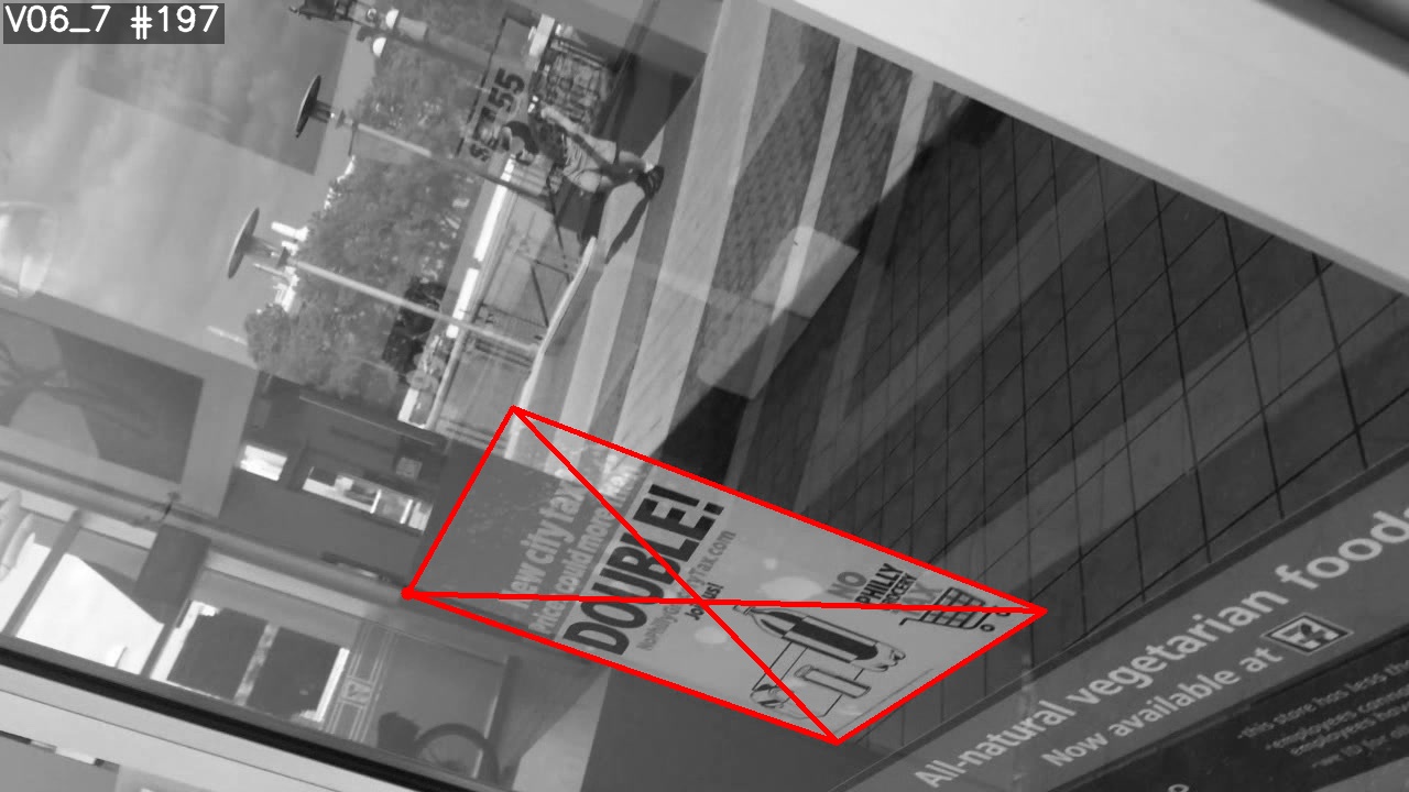
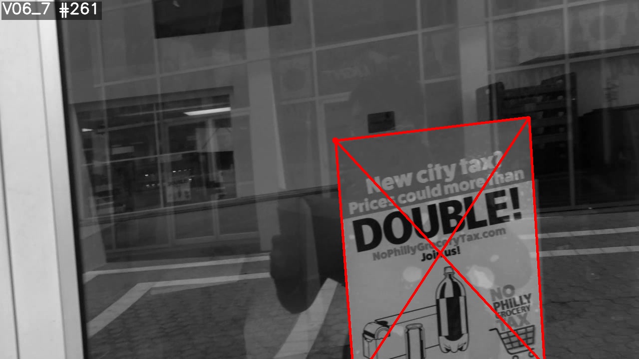
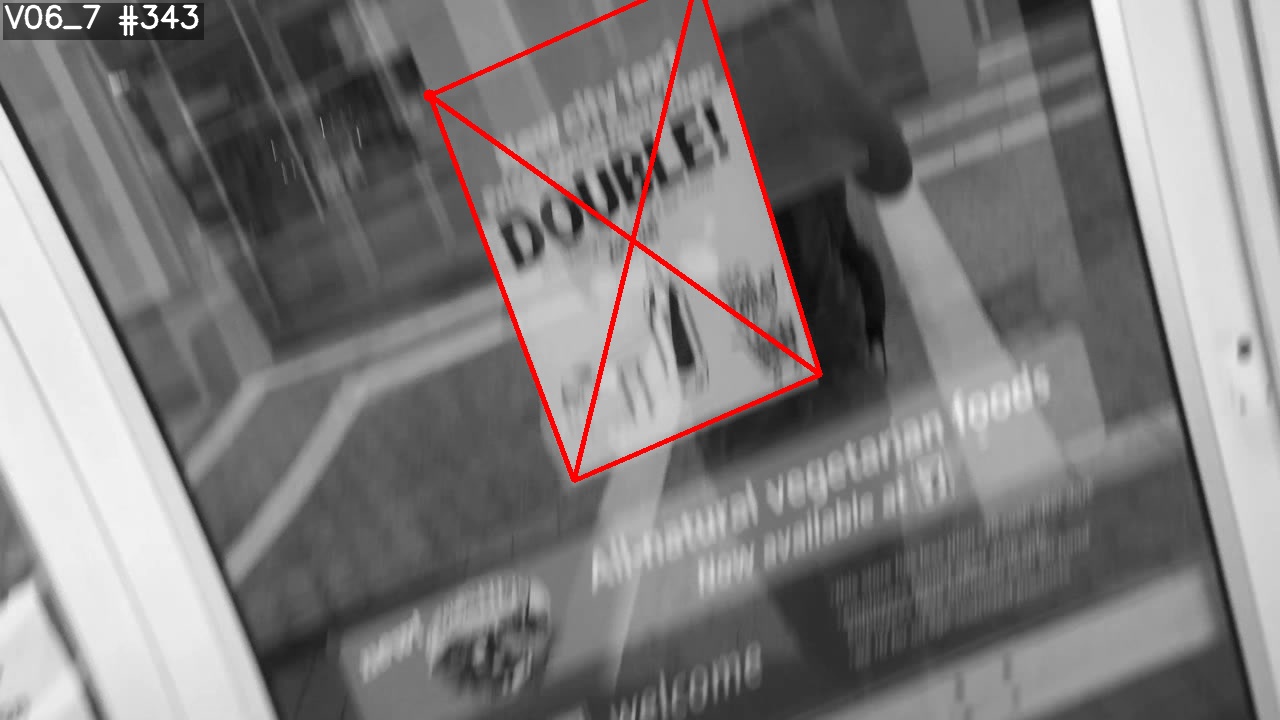
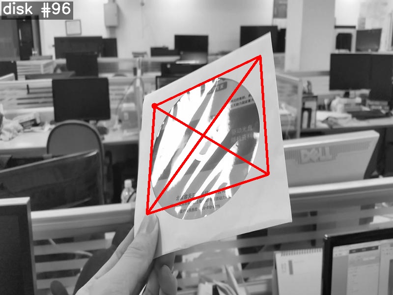
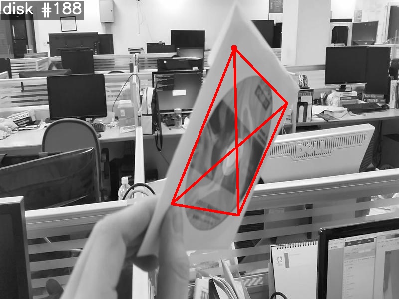
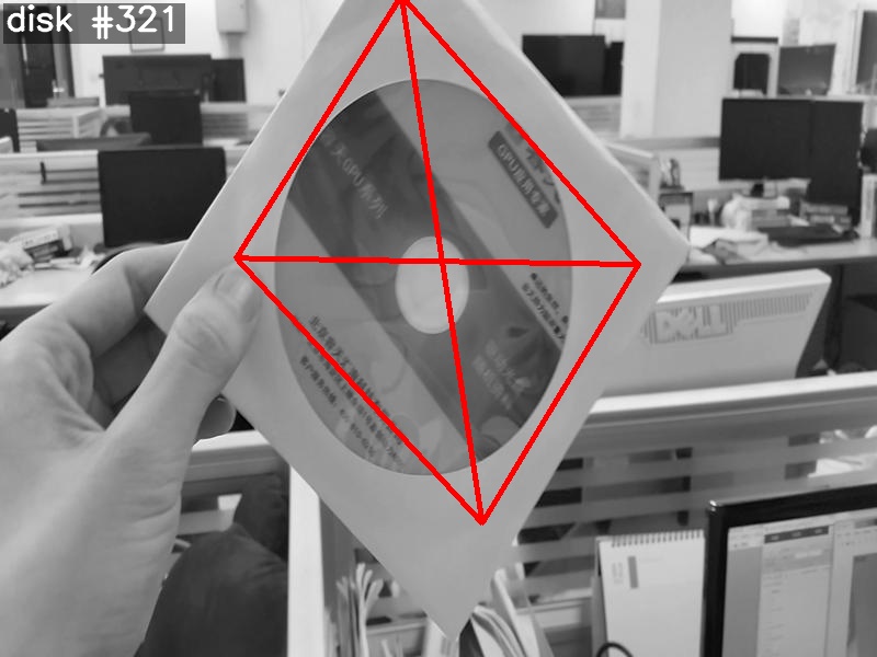
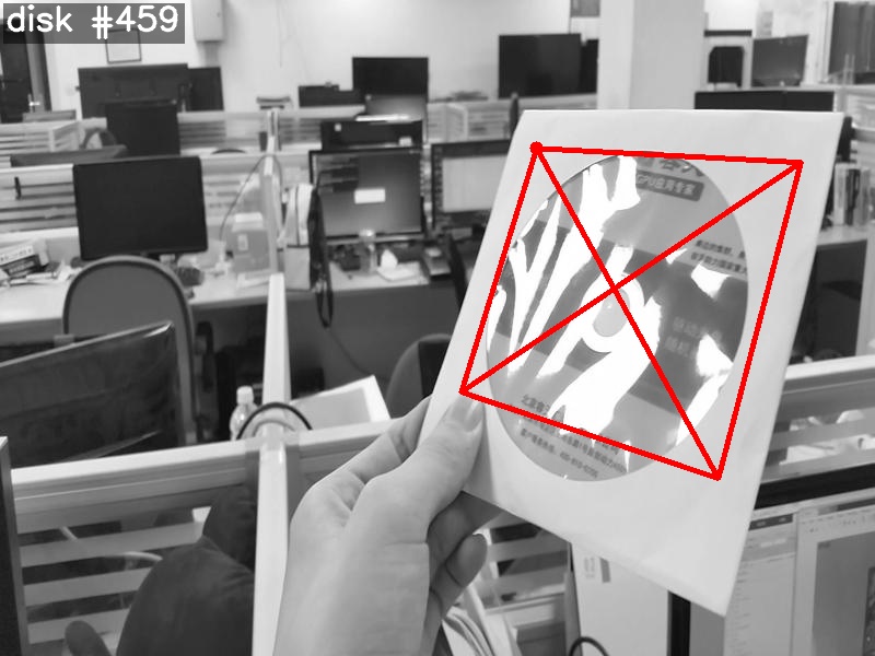
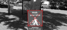
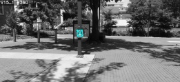
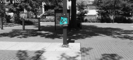
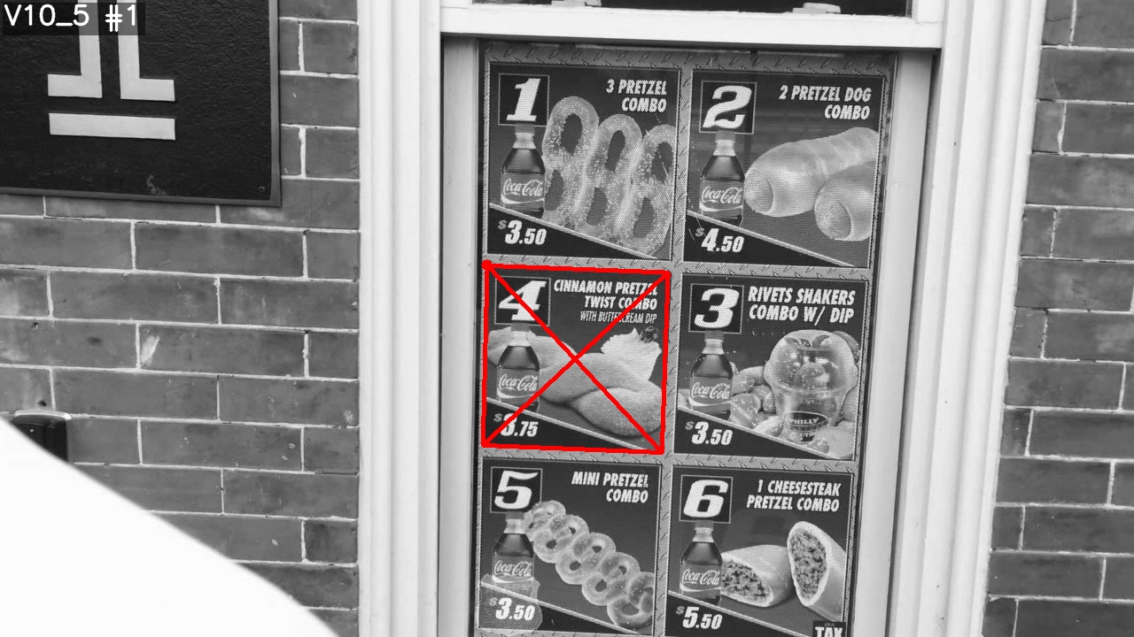
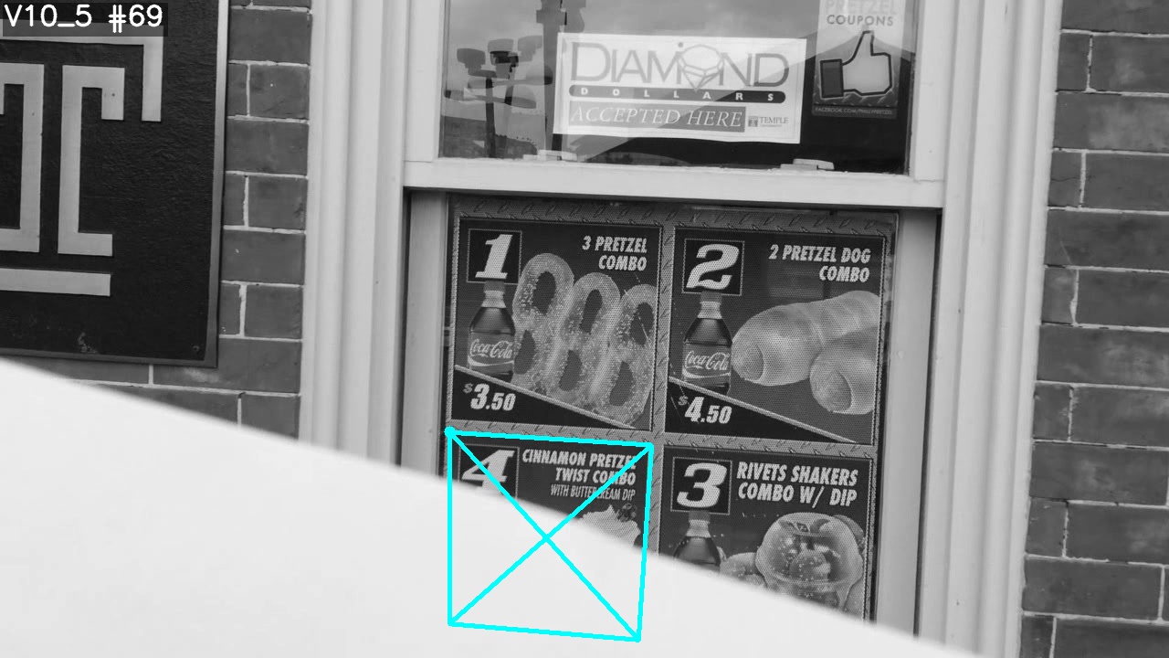
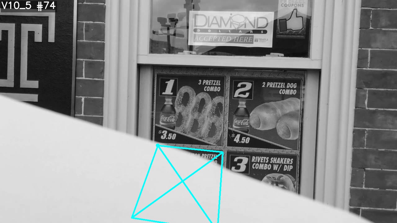
Figure 8: WOFT tracking. State visualization - red: tracking, cyan: lost - switch to local flow. First row: WOFT handles strong occlusions on the POT-210 V18_5 sequence. Second row: successful tracking on the V06_7 POT-210 unconstrained with perspective change, partial occlusion, scale change and motion blur. Third row: successful tracking in a POIC disk sequence, where a large part of the target surface changes appearance because of specular reflection. The last two rows show selected tracking failures. Row 4: the tracker is ‘lost‘ and did not recover because of a big scale difference w.r.t. the template frame, however, the local homography estimation prevents complete failure. Row 5: the target becomes almost fully occluded and the tracker switches to track a nearby distractor patch. Later WOFT reacquired the correct target. Last row: WOFT can handle a moderate amount of motion blur, but fails on extremely blurred frames.

4.5 POIC evaluation

We compare (Fig. 7) the WOFT tracker performance with the top methods evaluated on the POIC [7] dataset. Apart from the methods evaluated on POT-210, this includes SOL [14] and Bit-Planes [1]. WOFT achieves state-of-the-art results with $96.1$ P@5 and $98.0$ P@15. More results are in supplementary materials. See Fig. 8 for WOFT output examples on both POT-210 and POIC.

5 Discussion and Limitations

The WOFT tracker handles partial occlusions, a moderate amount of motion blur, and the illumination changes and lack of texture present in the POIC dataset. In comparison, other methods performing well on POIC (SiamESM [6], GOP-ESM [7]) have low performance on POT-210 and vice versa (LISRD [32], SIFT [27]). WOFT does not feature a re-detection scheme and estimates only the residual transformation after the pre-warp step. This causes issues when the tracker gets lost for more than 10 frames on the scale subset. After resetting the pre-warp source frame to $G=0$ (pre-warp with an identity homography), the scale component of the residual transformation is sometimes bigger than what the flow network can handle (see Fig. 8).

We tested the proposed WFH homography method on the RAFT OF network, which is accurate (Fig. 5), but slow (275ms per frame). However, the OF estimation is an active area of research and we expect new accurate and fast methods to be published in the future. The core idea of WFH – flow weights computed from an OF cost-volume and a differentiable homography estimation with weighted LSq – is applicable to other OF methods. The ablation study results with RAFT replaced by LiteFlowNet2 support this claim. We also proposed a simple WOFT_{$\downarrow\!3$} variant that operates fast (19.2 FPS) and still achieves state-of-the-art.

6 Conclusions

We proposed a novel formulation of deep homography estimation by weighted least squares. The weighted flow homography (WFH) module is differentiable and can be trained end-to-end together with an optical flow network that provides dense correspondences. A novel planar object tracker, called WOFT, that uses WFH was evaluated on two complementary planar object tracking benchmarks and sets a new state-of-the-art on POIC, POT-210, and POT-280. On POT-210 it outperforms all other published methods by a large margin. Inaccuracy of the POT-210 ground truth accounted for half of the WOFT errors. We publish the WOFT code, trained model and an improved GT annotation of a POT-210 subset.
Acknowledgements. This work was supported by Toyota Motor Europe, by CTU student grant SGS20/171/OHK3/3T/13, and by the Research Center for Informatics project CZ.02.1.01/0.0/0.0/16_019/0000765 funded by OP VVV.

References

- [1] Hatem Alismail, Brett Browning, and Simon Lucey. Robust tracking in low light and sudden illumination changes. In 2016 Fourth International Conference on 3D Vision (3DV), pages 389–398. IEEE, 2016.
- [2] Simon Baker and Iain Matthews. Lucas-kanade 20 years on: A unifying framework. International journal of computer vision, 56(3):221–255, 2004.
- [3] Herbert Bay, Andreas Ess, Tinne Tuytelaars, and Luc Van Gool. Speeded-up robust features (surf). Computer vision and image understanding, 110(3):346–359, 2008.
- [4] Selim Benhimane and Ezio Malis. Real-time image-based tracking of planes using efficient second-order minimization. In 2004 IEEE/RSJ International Conference on Intelligent Robots and Systems (IROS)(IEEE Cat. No. 04CH37566), volume 1, pages 943–948. IEEE, 2004.
- [5] Selim Benhimane and Ezio Malis. Homography-based 2d visual tracking and servoing. The International Journal of Robotics Research, 26(7):661–676, 2007.
- [6] Lin Chen, Yaowu Chen, Haibin Ling, Xiang Tian, and Yuesong Tian. Learning robust features for planar object tracking. IEEE Access, 7:90398–90411, 2019.
- [7] Lin Chen, Haibin Ling, Yu Shen, Fan Zhou, Ping Wang, Xiang Tian, and Yaowu Chen. Robust visual tracking for planar objects using gradient orientation pyramid. Journal of Electronic Imaging, 28(1):1–16, 2019.
- [8] Lin Chen, Fan Zhou, Yu Shen, Xiang Tian, Haibin Ling, and Yaowu Chen. Illumination insensitive efficient second-order minimization for planar object tracking. In 2017 IEEE International Conference on Robotics and Automation (ICRA), pages 4429–4436. IEEE, 2017.
- [9] Ondrej Chum and Jiri Matas. Matching with prosac-progressive sample consensus. In 2005 IEEE computer society conference on computer vision and pattern recognition (CVPR’05), volume 1, pages 220–226. IEEE, 2005.
- [10] Daniel DeTone, Tomasz Malisiewicz, and Andrew Rabinovich. Deep image homography estimation. arXiv preprint arXiv:1606.03798, 2016.
- [11] Heng Fan, Liting Lin, Fan Yang, Peng Chu, Ge Deng, Sijia Yu, Hexin Bai, Yong Xu, Chunyuan Liao, and Haibin Ling. Lasot: A high-quality benchmark for large-scale single object tracking. In Proceedings of the IEEE Conference on Computer Vision and Pattern Recognition, pages 5374–5383, 2019.
- [12] Martin A Fischler and Robert C Bolles. Random sample consensus: a paradigm for model fitting with applications to image analysis and automated cartography. Communications of the ACM, 24(6):381–395, 1981.
- [13] Xufeng Han, Thomas Leung, Yangqing Jia, Rahul Sukthankar, and Alexander C Berg. Matchnet: Unifying feature and metric learning for patch-based matching. In Proceedings of the IEEE conference on computer vision and pattern recognition, pages 3279–3286, 2015.
- [14] Sam Hare, Amir Saffari, and Philip HS Torr. Efficient online structured output learning for keypoint-based object tracking. In 2012 IEEE Conference on Computer Vision and Pattern Recognition, pages 1894–1901. IEEE, 2012.
- [15] R. I. Hartley and A. Zisserman. Multiple View Geometry in Computer Vision. Cambridge University Press, ISBN: 0521540518, second edition, 2004.
- [16] Kaiming He, Xiangyu Zhang, Shaoqing Ren, and Jian Sun. Deep residual learning for image recognition. In Proceedings of the IEEE conference on computer vision and pattern recognition, pages 770–778, 2016.
- [17] Tak-Wai Hui, Xiaoou Tang, and Chen Change Loy. A lightweight optical flow cnn—revisiting data fidelity and regularization. IEEE transactions on pattern analysis and machine intelligence, 43(8):2555–2569, 2020.
- [18] Matej Kristan, Ales Leonardis, Jiri Matas, Michael Felsberg, Roman Pflugfelder, Luka Cehovin Zajc, Tomas Vojir, Goutam Bhat, Alan Lukezic, Abdelrahman Eldesokey, et al. The sixth visual object tracking vot2018 challenge results. In Proceedings of the European Conference on Computer Vision (ECCV), 2018.
- [19] Matej Kristan, Aleš Leonardis, Jiří Matas, Michael Felsberg, Roman Pflugfelder, Joni-Kristian Kämäräinen, Martin Danelljan, Luka Čehovin Zajc, Alan Lukežič, Ondrej Drbohlav, et al. The eighth visual object tracking vot2020 challenge results. In European Conference on Computer Vision, pages 547–601. Springer, 2020.
- [20] Matej Kristan, Jiri Matas, Ales Leonardis, Michael Felsberg, Roman Pflugfelder, Joni-Kristian Kamarainen, Luka Cehovin Zajc, Ondrej Drbohlav, Alan Lukezic, Amanda Berg, et al. The seventh visual object tracking vot2019 challenge results. In Proceedings of the IEEE International Conference on Computer Vision Workshops, pages 0–0, 2019.
- [21] Matej Kristan, Jiří Matas, Aleš Leonardis, Michael Felsberg, Roman Pflugfelder, Joni-Kristian Kämäräinen, Hyung Jin Chang, Martin Danelljan, Luka Cehovin, Alan Lukežič, Ondrej Drbohlav, Jani Käpylä, Gustav Häger, Song Yan, Jinyu Yang, Zhongqun Zhang, and Gustavo Fernández. The ninth visual object tracking vot2021 challenge results. In Proceedings of the IEEE/CVF International Conference on Computer Vision (ICCV) Workshops, pages 2711–2738, October 2021.
- [22] Pengpeng Liang, Haoxuanye Ji, Yifan Wu, Yumei Chai, Liming Wang, Chunyuan Liao, and Haibin Ling. Planar object tracking benchmark in the wild. Neurocomputing, 454:254–267, 2021.
- [23] Pengpeng Liang, Yifan Wu, Hu Lu, Liming Wang, Chunyuan Liao, and Haibin Ling. Planar object tracking in the wild: A benchmark. In 2018 IEEE International Conference on Robotics and Automation (ICRA), pages 651–658. IEEE, 2018.
- [24] Tsung-Yi Lin, Michael Maire, Serge Belongie, James Hays, Pietro Perona, Deva Ramanan, Piotr Dollár, and C Lawrence Zitnick. Microsoft coco: Common objects in context. In European conference on computer vision, pages 740–755. Springer, 2014.
- [25] Yuan Liu, Zehong Shen, Zhixuan Lin, Sida Peng, Hujun Bao, and Xiaowei Zhou. Gift: Learning transformation-invariant dense visual descriptors via group cnns. Advances in Neural Information Processing Systems, 32, 2019.
- [26] Ilya Loshchilov and Frank Hutter. Decoupled weight decay regularization. In International Conference on Learning Representations, 2018.
- [27] David G Lowe. Distinctive image features from scale-invariant keypoints. International journal of computer vision, 60(2):91–110, 2004.
- [28] Bruce D Lucas and Takeo Kanade. An iterative image registration technique with an application to stereo vision. In Proceedings of the 7th international joint conference on Artificial intelligence-Volume 2, pages 674–679, 1981.
- [29] Dmitrii Matveichev and Daw-Tung Lin. Mobile augmented reality: Fast, precise, and smooth planar object tracking. In 2020 25th International Conference on Pattern Recognition (ICPR), pages 6406–6412. IEEE, 2021.
- [30] Matthias Muller, Adel Bibi, Silvio Giancola, Salman Alsubaihi, and Bernard Ghanem. Trackingnet: A large-scale dataset and benchmark for object tracking in the wild. In Proceedings of the European Conference on Computer Vision (ECCV), pages 300–317, 2018.
- [31] Ty Nguyen, Steven W Chen, Shreyas S Shivakumar, Camillo Jose Taylor, and Vijay Kumar. Unsupervised deep homography: A fast and robust homography estimation model. IEEE Robotics and Automation Letters, 3(3):2346–2353, 2018.
- [32] Rémi Pautrat, Viktor Larsson, Martin R Oswald, and Marc Pollefeys. Online invariance selection for local feature descriptors. In European Conference on Computer Vision, pages 707–724. Springer, 2020.
- [33] F. Perazzi, J. Pont-Tuset, B. McWilliams, L. Van Gool, M. Gross, and A. Sorkine-Hornung. A benchmark dataset and evaluation methodology for video object segmentation. In Computer Vision and Pattern Recognition, 2016.
- [34] Christian Pirchheim and Gerhard Reitmayr. Homography-based planar mapping and tracking for mobile phones. In 2011 10th IEEE International Symposium on Mixed and Augmented Reality, pages 27–36. IEEE, 2011.
- [35] Jordi Pont-Tuset, Federico Perazzi, Sergi Caelles, Pablo Arbeláez, Alex Sorkine-Hornung, and Luc Van Gool. The 2017 davis challenge on video object segmentation. arXiv preprint arXiv:1704.00675v2, 2017.
- [36] Esteban Real, Jonathon Shlens, Stefano Mazzocchi, Xin Pan, and Vincent Vanhoucke. Youtube-boundingboxes: A large high-precision human-annotated data set for object detection in video. In proceedings of the IEEE Conference on Computer Vision and Pattern Recognition, pages 5296–5305, 2017.
- [37] Ignacio Rocco, Relja Arandjelovic, and Josef Sivic. Convolutional neural network architecture for geometric matching. In Proceedings of the IEEE conference on computer vision and pattern recognition, pages 6148–6157, 2017.
- [38] Paul-Edouard Sarlin, Daniel DeTone, Tomasz Malisiewicz, and Andrew Rabinovich. Superglue: Learning feature matching with graph neural networks. In Proceedings of the IEEE/CVF Conference on Computer Vision and Pattern Recognition, pages 4938–4947, 2020.
- [39] Gilles Simon, Andrew W Fitzgibbon, and Andrew Zisserman. Markerless tracking using planar structures in the scene. In Proceedings IEEE and ACM International Symposium on Augmented Reality (ISAR 2000), pages 120–128. IEEE, 2000.
- [40] Karen Simonyan and Andrew Zisserman. Very deep convolutional networks for large-scale image recognition. CoRR, abs/1409.1556, 2014.
- [41] Fang Sun, Xiangyi Sun, Banglei Guan, Tao Li, Cong Sun, and Yingchao Liu. Planar homography based monocular slam initialization method. In Proceedings of the 2019 2nd International Conference on Service Robotics Technologies, pages 48–52, 2019.
- [42] Zachary Teed and Jia Deng. RAFT: Recurrent all-pairs field transforms for optical flow. In European Conference on Computer Vision, pages 402–419. Springer, 2020.
- [43] Yurun Tian, Xin Yu, Bin Fan, Fuchao Wu, Huub Heijnen, and Vassileios Balntas. SOSNet: Second order similarity regularization for local descriptor learning. In Proceedings of the IEEE/CVF Conference on Computer Vision and Pattern Recognition, pages 11016–11025, 2019.
- [44] Julien Valognes, Niloufar Salehi Dastjerdi, and Maria Amer. Augmenting reality of tracked video objects using homography and keypoints. In International Conference on Image Analysis and Recognition, pages 237–245. Springer, 2019.
- [45] Tao Wang and Haibin Ling. Gracker: A graph-based planar object tracker. IEEE transactions on pattern analysis and machine intelligence, 40(6):1494–1501, 2017.
- [46] Yi Wu, Jongwoo Lim, and Ming-Hsuan Yang. Object tracking benchmark. IEEE Transactions on Pattern Analysis and Machine Intelligence, 37(9):1834–1848, 2015.
- [47] Ning Xu, Linjie Yang, Yuchen Fan, Dingcheng Yue, Yuchen Liang, Jianchao Yang, and Thomas Huang. Youtube-vos: A large-scale video object segmentation benchmark. arXiv preprint arXiv:1809.03327, 2018.
- [48] Rui Zeng, Simon Denman, Sridha Sridharan, and Clinton Fookes. Rethinking planar homography estimation using perspective fields. In Asian Conference on Computer Vision, pages 571–586. Springer, 2018.
- [49] Xinrui Zhan, Yueran Liu, Jianke Zhu, and Yang Li. Homography decomposition networks for planar object tracking. In Proceedings of the AAAI Conference on Artificial Intelligence, volume 36, pages 3234–3242, 2022.
- [50] Kaixiang Zhang, Jian Chen, and Bingxi Jia. Asymptotic moving object tracking with trajectory tracking extension: A homography-based approach. International Journal of Robust and Nonlinear Control, 27(18):4664–4685, 2017.