This paper provides an overview of the Pythagorean centrality measures, which are the arithmetic, geometric, and harmonic means. Both the evolution of their meaning through history and their geometrical interpretation are outlined. Relevant examples of use cases for each of them are introduced, spanning a variety of areas of knowledge. Their differences and similarities are explored. Finally, the issue of which mean to use in different situations in order to make advantageous predictions is addressed.
Keywords: central tendency, Pythagorean means, arithmetic mean, geometric mean, harmonic mean, data selection.

1 Introduction

The concept of the mean of a set of measurements was known in civilizations before our era. Its meaning has evolved over time, according to needs. In ancient India, Rituparna estimated the number of leaves on a tree based on a single twig, which he multiplied by the estimated number of twigs on the branches. This can be seen as an intuitive predecessor to the arithmetic mean, as the leaf count of a single twig was taken to be representative of any other twig [1]. During the civilization of the ancient Greeks, the Pythagoreans found several mathematical formulations of the mean which can give different values for the same two numbers [4]. The 9th-century mathematician Al-Kindi introduced cryptography which used several statistical concepts including the relative frequency and the arithmetic mean [5]. The 16th and 17th centuries brought a shift in paradigm that led to the arithmetic mean being viewed as the ”true” mean in the eyes of most people [4].

In our current knowledge, given the non-negative measurements $x_{1}<\cdots<x_{n}$, the mean can be any value between $x_{1}$ and $x_{n}$ [6]. However for practical reasons, a requirement is mandatory in order to target one value among all the values. The requirement is often expressed by informal arguments, such as the mean value must greatly resemble other measurements, or that it must be the closest to the others, or the one that expresses a trend of the phenomenon, or the value that compensates for errors such as the additive noise in a signal. No matter how the informal requirement is expressed, the mean value is the closest to the measurements, up to some transform, according to some criterion, e.g. the value $\mu$ minimizing the quadratic error $\sum_{i=1}^{n}(T(x_{i})-O(\mu))^{2}$, where $T()$ and $O()$ are some transforms. One may think that in order to sidestep an arbitrary choice of a value as a mean among all, it is enough to determine the value that satisfies a predefined criterion. But it is not so, because there can be an infinity of criteria. In other words, we are not escaping arbitrariness altogether, but moving from a type of arbitrariness where the mean is in $[x_{1},x_{n}]$ to an agreed arbitrariness where the mean value fulfils some criterion chosen arbitrarily among many others. Despite the arbitrariness, the mean is a concept that many among us claim to know and is the basis of reasoning in various fields. It is widely used for purposes such as determining the price evolution of consumer products, estimating the Human Development Index, evaluating students learning, measuring the daily air temperature in a city, and calculating the capacitance of several capacitors connected in series. The goal of this paper is to examine Pythagorean centrality measures: the arithmetic mean (AM), the geometric mean (GM), and the harmonic mean (HM). For this purpose, we will describe these three means as a finite set of non-negative measurements and explore the relationship between them, their history, and their use. Moreover, we will propose a geometric interpretation of the three means in terms of dimensions of hyperrectangles as well as a statistical interpretation in terms of data selection. The next section is devoted to the definition and the usefulness of Pythagorean centrality measures. Their history and the comparison between them are described in Section 3. In Section 4, we present the means as a mechanism of data selection. Examples of use cases are in section 5.

2 Pythagorean centrality measures

The term Pythagorean centrality measures encompass the arithmetic, geometric, and harmonic means. In all this study, we limit ourselves to the case of non-negative measurements. Given $n$ scalar measurements $x_{1}<\cdots<x_{n}$, the interpretation given our current knowledge would suggest that a Pythagorean centrality measure is located between $x_{1}$ and $x_{n}$ [6] and is related to compensation of errors, tendency, balance, and representativeness. These qualifications can be considered synonymous because all can be couched as the value $\mu$ minimizing a criterion based on the squared error; i.e. $\sum_{i=1}^{n}w_{i}(T(x_{i})-O(\mu))^{2}$, where $T()$ and $O()$ are some transforms. The non-negative weight $w_{i}$ of $x_{i}$ can be interpreted as its relative frequency, the empirical probability of observing it, and its relevance according to a certain criterion. In what follows, we will use centrality, trend, and mean interchangeably and focus only on the mean of a finite set of measurements. In reality, the geometric (resp. harmonic) mean is also an arithmetic mean of measurements transformed by logarithmic (resp. inverse) transform as shown in Table 2. In both these cases, the measurements in the original space are transformed, the arithmetic mean is calculated in the transformed space, and then the mean is transported back to the original space. The squared-error-based criterion to be minimized is expressed in the transformed space. As we will see later, this formalization of the Pythagorean centrality measures in Table 2 makes it possible to explain one of the data selection mechanisms.

	AM	GM	HM
Criterion	$min_{a}\sum_{i=1}^{n}w_{i}(y_{i}-a)^{2}$, $w_{i}\geq 0$ $\forall i$, and $\sum_{i=1}^{n}w_{i}=1$
Data transform	y=x	$y=ln(x)$	$y=1/x$
Parametrization	$a=\mu$	$a=ln(\mu)$	$a=1/\mu$
Mean ($\mu$)	$\sum_{i=1}^{n}w_{i}x_{i}$	$\prod_{i=1}^{n}x_{i}^{w_{i}}$	$1/(\sum_{i=1}^{n}w_{i}/x_{i})$

Table 2: Pythagorean centrality measures: the minimization problem by which each is derived, the data transform, the parametrization used, and the mean.

Most humans default to the arithmetic mean when asked to find the average of a sample. During an undergraduate class in computer science, 30 students were asked to calculate the mean of three numbers. As expected, all calculated the arithmetic mean and no one thought of using another measure of centrality. There are countless examples of everyday use for the arithmetic mean, such as the estimation of marks obtained by students, the daily temperature, the position of a centre of mass [10], and the Consumer Product Index (CPI) [36]. It is easy to compute and understand, and, unlike the other two means, it does not require a transformation of measurements. The arithmetic mean is suitable for indicating the tendency when the dispersion of measurements is not high. For the compensation of errors, a noisy measurement can be replaced by the arithmetic mean estimated from the closest measurements in the case of uncorrelated and additive noise [31]. However, it is sensitive to extreme values. For example, let’s assume that the five equally-weighted measurements of the daily temperature reported are 8, 13, 14, 10, and 1000 degrees. Although 1000 degrees is clearly a mistake, it influences the average daily temperature, resulting in an unrealistic value: 209 degrees. This sensitivity of the arithmetic mean may explain why the geometric mean has regained popularity in many areas of knowledge. In physics, it expresses the relationship between the classical and the relativistic Doppler effect [13]. In image processing, a geometric filter based on the geometric mean is used for the reduction of speckle in radar images [16]. As a filter, the geometric mean weakens the contribution of high values heavily corrupted by multiplicative noise. In finance, the geometric mean is used to characterize the growth rates of an investment [17]. It is also used to assess the effectiveness of a vaccine [11]. The CPI is estimated using the geometric mean for certain products, as will be discussed below. The harmonic mean is used for change detection in radar images [20], estimation of the average velocity over a trip [21], averaging the financial multiples with price in the numerator [23], estimation of the pollutant load that can be permitted in a water quality limited stream [18], and estimation of the properties of a heterogeneous system of porous media [18]. In the case of multiples, the harmonic mean can provide more accurate estimates than the arithmetic mean. This surprising result has been addressed several times in litigation in the United States [19]. The geometric and harmonic means favour small values and are therefore less sensitive than the arithmetic mean to larger outliers. In the example presented above the arithmetic mean is 209 degrees while the geometric and harmonic means are around 27.02 and 13.36 degrees, respectively. While the former is far from the median, which is 13 degrees, the latter is close to it.

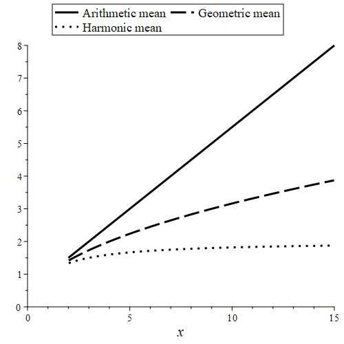
Figure 1: The three means of 1 and x.

Finally, the three means can be ranked. To illustrate this, the three means of 1 and $x$ are plotted in Fig. 1 as a function of $x\in[2,15]$. It can be observed that the means are contained in the interval $[0,x]$ and AM $>$ GM $>$ HM. The inequality is valid for any finite number of measurements. The reader can find the formal proof in [24].

3 Evolution of the Pythagorean centrality measures

Note that historical clarification is required to summarize what was defined by Pythagoras, his disciples and what has been introduced afterwards. For example, in [9], it is stated that the geometric mean was introduced at the beginning of the 19th century. For this purpose, the history of the three means and the current geometrical interpretation are the focus of this section.

3.1 History

The arithmetic, geometric, and harmonic means of a sample appeared during the last centuries BCE. The Babylonians used the arithmetic mean in astronomy [25], classical Greek music theorists employs the geometric mean in tuning instruments [26], and the harmonic mean is the basis of a solution of a division of loaves of bread by 10 [28]. However, it was in ancient Greece that the study of the mean figured prominently because Greek mathematics was primarily concerned with proportions, as is the case with ratios and the Pythagorean theorem. The remarkable contributions of Pythagoras in the study of proportions probably led to the three measures of centrality attributed to Pythagoras and his disciples, i.e. Pythagorean means [22]. Much later, Al-Kindi introduced cryptography in the 9th century, using several statistical concepts, including relative frequency and arithmetic mean [5]. In the 11th century, Al-Biruni used the midrange as a mean in astronomy [4]. Until the end of the Middle Ages, the notion of mean had several interpretations. One of these was the midrange [29], which is the value located equidistant from the two extreme values. This is not easily generalizable to the case of more than two measurements, which is why the definition of the arithmetic mean of a sample as we know it today was not proposed until the 16th century [4]. There is no consensus on the origin of the arithmetic mean of a population (i.e. the mathematical expectation). Some date it to the 17th century, attributing it to Blaise Pascal. Regardless, it was only formalized in the 19th century, by Laplace [30]. Also in the Middle Ages, the harmonic mean was used to solve what is commonly called the cistern mathematical problem that appeared in Europe and India [27]. Details regarding the development of the harmonic mean after this time period seem to be lacking in the literature. The geometric mean as we know it was not proposed until the beginning of the 19th century [9]. Surprisingly, the population geometric mean was only introduced in 2013 [9]. Note that the geometric and arithmetic means have been combined to form the arithmetic-geometric mean used in the calculation of integrals [32, 33]. As its name suggests, this average consists of iteratively calculating the arithmetic and geometric mean of the measurements.

3.2 Geometric interpretation

The geometric interpretation is only provided for equal weights measurements. Let us consider a sample of only two values, $x_{1}$ and $x_{2}$ with equal weights. The three means can be represented geometrically using a circle of diameter $x_{1}+x_{2}$, as depicted in Fig. 2.

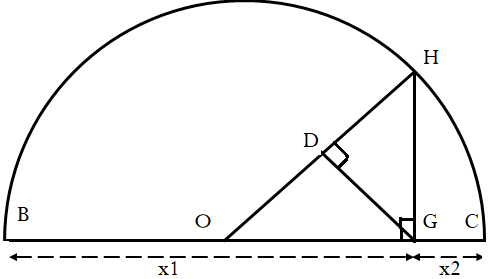
Figure 2: Representation of the three means of two numbers.

The lengths of BG and GC are $x_{1}$ and $x_{2}$, respectively. The arithmetic mean coincides with the radius of the circle (OH), HG corresponds to the geometric mean, and HD to the harmonic mean [2]. This relationship among the three means is only applicable to two numbers. We suggest an alternative geometric interpretation that can be applied to more than two numbers $(n\geq 2)$. Let us consider the hyperrectangle $R_{n}$, where $x_{1}$, …, $x_{n}$ are its dimensions. In $R_{n}$, there is a total of $2^{(n-1)}n$ edges. As a result, each edge is repeated $2^{(n-1)}$ times. For instance, in $R_{3}$, each one of the 3 edges would be repeated 4 times. The hyperperimeter of $R_{n}$ is given by:

$$P_{n}=2^{(n-1)}(x_{1}+x_{2}+...+x_{n})$$ (1)

According to this formula, the hyperperimeter is the arithmetic mean multiplied by a factor whose value is contingent on the number of dimensions:

$$AM=\frac{P_{n}}{2^{(n-1)}n}$$ (2)

The hypervolume $V_{n}=x_{1}x_{2}...x_{n}$ of $R_{n}$ is the geometric mean raised to the n^th power:

$$GM=\sqrt[n]{V_{n}}$$ (3)

The hyperrectangle $R_{n}$ is made up of $n$ pairs of equal $(n-1)$-dimensional hyperrectangles. For example, in $R_{3}$, there are 6 rectangles that are equal to one another two by two. Let us consider the $j^{th}$ hyperrectangle $R_{n-1,j}$ with hypervolume $V_{n-1,j}=\prod\limits_{i\neq j}^{n}x_{i}$. The arithmetic mean of the hypervolumes of the $2n$ hyperrectangles $R_{n-1,j}$ is:

$$A_{n}=\frac{1}{2n}\sum^{2n}_{j=1}V_{n-1,j}=\frac{1}{n}\sum^{n}_{j=1}V_{n-1,j}$$ (4)

The harmonic mean is expressed in terms of a ratio between the hypervolume of $R_{n}$ and the arithmetic mean of the hypervolumes of these n $R_{n-1}$:

$$H_{n}=\frac{V_{n}}{A_{n}}$$ (5)

In other terms, this is the ratio between the geometric mean of edges to the power of $n$ and the arithmetic mean $A_{n}$ of the hypervolumes of $n$ hyperrectangles of dimension $n-1$. To conclude, the geometric interpretation of the three Pythagorean centrality measures leads to translate the inequality between them into an inequality between geometric primitives of a hyperrectangle.

4 Data selection

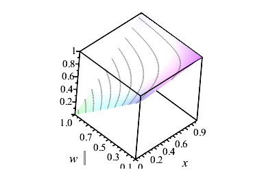
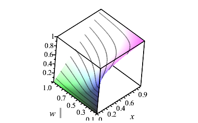
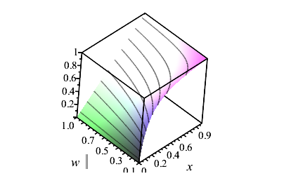
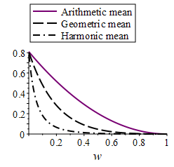
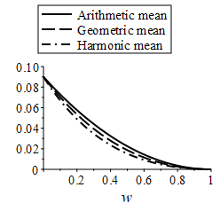
Figure 3: Weighted Pythagorean centrality measures of 1 and $x$ as a function of $x$ and the weight $w$ of $x$. The upper row shows the arithmetic, geometric, and harmonic means respectively. The bottom row shows the velocities of the means when $x=0.1$ (left) and $x=0.7$ (right).

Remember that the non-negative weight $w_{i}$ of $x_{i}$ encodes its relative frequency, the empirical probability of observing it, or its relevance according to a certain criterion. Let us call it, the w-weight. When estimating the mean, the w-weights implement a selection mechanism for measurements, since they indicate how each of them contributes to the estimated mean. Note that the selection of a measurement is not taken in the sense of all-or-nothing. Assigning a weight to a measurement is a selection since the measurement’s contribution is strengthened or weakened depending on this weight [12, 3, 34]. Fig. 3 displays the three weighted means of two numbers 1 and $x$, by varying $x\in[0,1[$ and the weight $w\in]0,1]$ of $x$. For the three weighted means, the more $w$ increases, the more strongly they are attracted by $x$. The difference between the three means is explained by the velocity at which each move towards $x$ as $w$ increases. For a given $w$, the velocity of a mean can be set to the square of the difference between the mean and $x$. Fig. 3 presents the velocities of the three means for $x=0.1$ and $x=0.7$. For a small $x$, the harmonic mean approaches $x$ more quickly than the geometric mean which in turn approaches $x$ more quickly than the arithmetic mean. This explains why the harmonic mean is the most sensitive to small values. When $x$ increases, the difference between the velocities of the three means is reduced.

We propose to make explicit another mechanism for selecting measurements which does not seem to have been made explicit before. The mechanism is expressed in the original space (the measurement space). For the sake of simplicity, first we consider that all measurements have the same w-weight. Let us return to the measurements $x_{1}<\cdots<x_{n}$. A centrality measure can be seen as a value belonging to the interval $[x_{1},x_{n}]$, where each of the measurements contributes to its identification. The closer a measure is to it, the more influence it has on it to keep it close. This conception implicitly establishes an analogy with the Coulomb’s law; i.e. both $x$ and the mean are seen as electric charges whose force of attraction decreases with the square of the distance between them. This analogy leads to basing attraction on the Euclidean distance $d(x,\mu)$ between a measurement $x$ and a Pythagorean centrality measure $\mu$ of the measurements. Since the influence of $x$ on $\mu$ decreases as $d(x,\mu)$ increases, an attraction function can be any decreasing function on $d(x,\mu)$, such as a Cauchy or Gaussian pdfs. Fig. 4 presents an example of the attraction function, which we call the Cauchy attraction function $f_{p}(x)=\frac{d^{2}(x_{n},x_{1})}{d^{2}(x,\mu_{p})+1}$, where $d^{2}(a,b)=(a-b)^{2}$ and $p~{}\in$ {arithmetic, geometric, harmonic}. The squared distance $d^{2}(x_{n},x_{1})$ is the range of measurements used as the normalization constant. In the denominator, one is added to $d^{2}()$ in order to avoid division by zero.

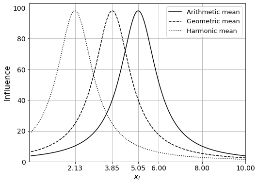
Figure 4: The attraction functions over the three central tendencies obtained by regular sampling of $[0.1,10]$.

Fig. 4 depicts the attraction functions obtained by regular sampling of $[0.1,10]$. The arithmetic, geometric, and harmonic means are around 5.05, 3.85, and 2.13 respectively. It can be noted that the measurements close to the means have the greatest attraction, regardless of the means used. The attraction of high values is higher in the case of the arithmetic mean. For example, the attraction function of the arithmetic mean at $x=10$ is greater than that of the geometric mean, which in turn is greater than that of the harmonic mean. Conversely, at $x=0.1$ the attraction function of the harmonic mean is greater than that of the geometric mean which in turn is greater than that of the arithmetic mean. Let us examine how the two selection mechanisms (w-weights and attraction function) can be combined. The combination is straightforward because the weighted attraction function can be either Cauchy $f_{p}(x_{i})\propto 1/(w_{i}d^{2}(x_{i},\mu_{p})+1)$ or Gaussian with a non-constant variance $g_{p}(x_{i})\propto exp(-w_{i}(x_{i}-\mu_{p})^{2})$. Fig. 5 shows the student grades and the Cauchy weighted attraction functions for the three means. The observations deduced from Fig. 4 remain valid. Moreover, the data are noisy which explains the difference between the weighted attraction functions at the maximum points.

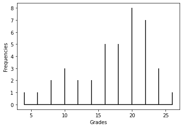
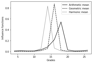
Figure 5: Frequencies of student grades and the three weighted attraction functions over the three central tendencies.

The third data selection mechanism is implemented by performing transformations to calculate geometric and harmonic means (see Table 2). Indeed, these two transformations modify the measurements in such a way as to enhance some and weaken the others. For example, the logarithm accentuates the difference between small values and attenuates the difference between large values. Someone may think that the inverse transform neutralizes the effects of the measurements transform. However, the back-transformed arithmetic mean calculated in the transformed space does not cancel the transformation of the measurements because the two transformations are not linear.

To conclude, a weighted mean implements three data selection mechanisms. One of the mechanisms is based on a frequency or any priori knowledge and the two other on the measurement itself. Thus, choosing which Pythagorean centrality measure to use defines how the measurements are considered and which ones are relevant. It follows that the right choice of a mean can be the cause of appropriate subsequent use of measurements such as accurate predictive analysis and fair decision-making.

5 Applications

5.1 Predictions

Let’s take the example of an airline that needs to estimate the optimal number of additional tickets to sell [35]. These seats are those purchased by passengers, called no-shows, who do not show up for a flight. For estimation purposes, the number of no-shows must be predicted as accurately as possible, because prediction errors lead to financial losses for the airline. A free seat is a loss of earnings and an oversold seat means that a person will be compensated for not boarding. To make the prediction, the airline uses the number of no-shows per flight over the last 200 flights. These data are indicated in Table 3. For each number of no-shows, the table gives the number of flights and the relative frequency of these flights, considered as an empirical probability of the flights.

No-shows	1	2	3	4	5	6	Total
Number of flights	70	40	10	20	20	40	200
Probability	0.35	0.20	0.05	0.10	0.10	0.20	1

Table 3: Number of no-shows on the last 200 flights, the number of flights per number of no-shows, and the empirical probability of the flights.

The prediction is made by a consultant whose compensation is linked to the accuracy of the predictions. If $x$ is the expected number of ”no-shows” and $n$ the actual number, the compensation is given by the following gain function expressed in a transformed space:

$$g(x,n)=1000-30(T(x)-T(n))^{2}$$ (6)

As shown in the table 2, $T(a)=a$ gives the arithmetic mean, $T(a)=ln(a)$ the geometric mean, and $T(a)=1/a$ the harmonic mean. Because $n$ is unknown, a way of finding the prediction $x$ is to use the expectation of the gain function, named the return function.

$$R(x)=1000-\sum\limits^{6}_{n=1}30(T(x)-T(n))^{2}pr(n)$$ (7)

Because $T()$ is invertible, maximizing $R(x)$ w.r.t $x$ allows to find the best predictor:

$$x^{*}=T^{-1}(\sum\limits^{6}_{n=1}T(n)\text{pr}(n))$$ (8)

Table 4 provides the three return functions, their maximum values, and the best predictors. For the consultant, the harmonic mean is the best scenario, since it allows her or him to earn more. In the absence of ground truth and other economic data, it is difficult to choose the best predictor for the airline. However, the airline could object to the use of a return function and therefore a central tendency measure.

Return function $R(x)$	Best predictor $x^{*}$	Best return $R(x^{*})$
$1000-30\sum_{n=1}^{6}(x-n)^{2}pr(n)$	AM = 3.00	883.00
$1000-30\sum_{n=1}^{6}(ln(x)-ln(n))^{2}pr(n)$	GM=2.34	984.26
$1000-30\sum_{n=1}^{6}(1/x-1/n)^{2}pr(n)$	HM=1.83	996.27

Table 4: Return functions expressed in the original and transformed spaces of data, their maximum values, and their best predictors

5.2 Consumer Price Index

We briefly describe the case of Canada. The CPI represents price change by comparing, over time, the cost of the same basket of goods and services. For decades, it was calculated using different formulas, including the arithmetic mean, but since 1995, for many products, the geometric mean has been used [36]. The arithmetic mean is still used for three out of 691 products (rents, tuition, and passenger vehicle insurance premiums) on the grounds that they are unlikely to have outliers. It is also used to group products into broader categories, such as food, housing and transport and to calculate the all-items CPI. The idea of using the geometric mean instead of the arithmetic mean to estimate CPI was put forward by economist W. S. Jevons in 1863 [7]. Later, however, he proposed the use of the harmonic mean instead. The reason for this choice was never explicitly stated in his published work [8]. Let’s examine the effect of Pythagorean centrality on the CPI using Canadian data acquired during the two years 2002 and 2017. Note that, the Canadian government tracks a wide variety of products and services. Based on consumer habits, weights are assigned to products indicating their importance to consumers. Table 5 summarizes the weights of the individual product groups and their CPIs in 2017, taking 2002 as the reference period. Table  6 shows the overall CPI as a function of Pythagorean centrality measures. As expected, the highest CPI is given by the arithmetic mean and the lowest by the harmonic mean. The latter is 1.3% lower than the CPI based on the arithmetic mean. It seems that there are not yet formal arguments to choose the central tendencies to use for the calculation of the CPI. This could open the door to arbitrariness and arguments of a political nature. Nevertheless, a good understanding of data selection could guide the choice of the appropriate central tendencies.

Product group	Weight	CPI
Food	0.1648	141.5
Shelter	0.2736	137.8
Household operations,	0.1280	121.4
furnishings, and equipment
Clothing and footwear	0.0517	91.1
Transportation	0.1995	133.0
Health and personal care	0.0479	123.4
Recreation, education, and reading	0.1024	111.3
Alcohol, beverages, tobacco,	0.0321	158.7
products, and cannabis

Table 5: Weights and CPI associated with each basket category as of January 2017 [37, 38].

Arithmetic mean	Geometric mean	Harmonic mean
130.20	129.40	128.50

Table 6: All-items CPI given by the three Pythagorean means.

5.3 Ellipse fitting

Fitting ellipses to given points is a problem that arises in computer graphics, remote sensing, geology, environment, and statistics, among many others. Different ideas have been implemented, including least-squares error minimizing and probability density estimation [39, 14, 15]. For 2D scatter points, we want to estimate an enclosing ellipse. An ellipse is defined by its centre and its principal axes. The centre can be estimated by using a Pythagorean centrality measure of the coordinates of the points. The directions of the principal axes are the eigenvectors of the covariance matrix estimated in the original data space or in the transformed space and transported back to the original space. The lengthening of the ellipse on each of the two axes is determined by the eigenvalues of the covariance matrix. Each of the three means is used for the calculation of both the center of mass and the principal axes of the ellipse. We can see in Fig. 6 that the direction of the principal axes of the ellipses is almost the same, but there is no spatial coincidence of their centres. This is expected because the harmonic mean and the associated ellipse are shifted toward the origin of the data space while the arithmetic mean and the associated ellipse are the farthest.

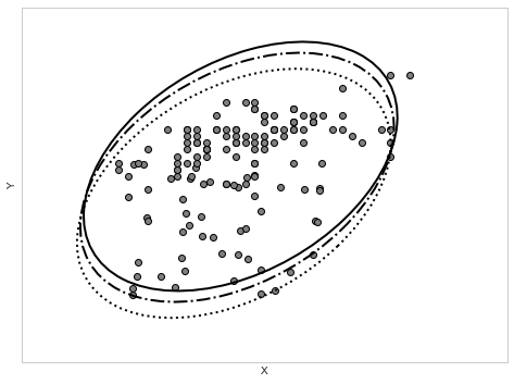
Figure 6: Ellipses obtained by using the arithmetic mean (solid), geometric mean (-.), and harmonic mean (..).

Conclusion

The arithmetic, geometric, and harmonic means make it possible to estimate the centrality of measurable phenomena. The arithmetic mean is the most used. The use of geometric and harmonic means reduces the influence of large measurements because they give greater influence to small measurements, which leads to the inequality: AM $>$ GM $>$ HM. Initially, this inequality was displayed in the case of the central tendencies of two measurements. We have provided a generalization that gives a geometric interpretation of these means in the case of several measurements. Through examples, we have shown the importance of selecting the appropriate mean in the sale of airline tickets, the ellipse estimation, and the estimation of the Consumer Price Index. We have also explained three data selection mechanisms implemented by Pythagorean means. It should be noted that the choice of the mean has been the subject of several lawsuits. Ultimately, this paper is just a brief overview of the concept of Pythagorean centrality measures. Much remains to be done to understand and better exploit the concept of centrality for data selection. For example, it’s hard to summarize and fully understand a set of measurements by using a single centrality measure. Selecting measurements using different centrality measures could provide a more complete picture of data.

References

- [1] A. Bakker. The Early History of Average Values and Implications for Education. Journal of Statistics Education 11, 2003.
- [2] C. Alsina and R. Nelsen. Math Made Visual: Creating Images for Understanding Mathematics. Mathematical Association of America, 2006.
- [3] M.W. Ayech, D. Ziou. Segmentation of Terahertz imaging using k-means clustering based on ranked set sampling. Expert Systems with Applications 42, pp. 2959-2974, 2015.
- [4] C. Eisenhart. The Development of the Concept of the Best Mean of a Set of Measurements from Antiquity to Present Day. Annual Meeting of the American Statistical Association, 1971.
- [5] L. D. Broemeling. An Account of Early Statistical Inference in Arab Cryptology. The American Statistician 4, pp. 255-257, 2011.
- [6] J. M. Borwein and P. B. Borwein. Pi and the AGM: A Study in the Analytic Number Theory and Computational Complexity. Wiley-Interscience, 1987.
- [7] W. S. Jevons. A Serious Fall in the Value of Gold Ascertained: And Its Social Effects Set Forth. E. Stanford, 1863.
- [8] F. Coggeshall. The Arithmetic, Geometric, and Harmonic Means. The Quarterly Journal of Economics 1, p. 83-86 , 1886.
- [9] R. M. Vogel. The geometric mean? Communications in Statistics - Theory and Methods 51, pp. 82-9, 2022.
- [10] J. R. Taylor. Mécanique classique. De Boeck supérieur, 2012.
- [11] K. A. Earle et al. Evidence for antibody as a protective correlate for COVID-19 vaccines. Vaccine 39, pp. 4423-4428, 2021.
- [12] S. Boutemedjet, D. Ziou. and N. Bouguila. Unsupervised Feature Selection for Accurate Recommendation of High-Dimensional Image Data. NIPS, pp. 177-184, 2007.
- [13] E. Baird. Special relativity considered as an average of earlier theories. Research Gate, 2020.
- [14] K. C. Chen, N. Bouguila, D. Ziou. Quantization-free parameter space reduction in ellipse detection. Expert Systems with Applications 38, pp. 7622-7632, 2011.
- [15] A. B. Goumeidane, D. Ziou, and N. Nacereddine. Scale Space Radon Transform for Non Overlapping Thick Ellipses Detection. Int, Conf. on Image Processing Theory, Tools and Applications (IPTA), pp. 1-6, 2022.
- [16] N. Gasnier, L. Denis, and F. Tupin. On the use and denoising of the temporal geometric mean for SAR time series. IEEE Geoscience and Remote Sensing Letters, 2021.
- [17] J. Hull. Options, futures and other derivatives. Pearson Education, 2015.
- [18] J. F. Limbrunner, R. M. Vogel, and L. C. Brown. Estimation of Harmonic Mean of a Lognormal Variable. Journal of Hydrologic Engineering 5, pp. 59-66, 2000.
- [19] G. E. Matthews. When Averaging Multiples, the Arithmetic Mean Is Inferior to the Harmonic Mean. Business Valuation Review 40, pp. 61–67, 2021.
- [20] G. Quin, B. Pinel-Puysségur, and J.-M. Nicolas. Comparison of Harmonic, Geometric and Arithmetic means for change detection in SAR time series. European Conference on Synthetic Aperture, pp. 255-258, 2012.
- [21] R. Falk, A. Lann, and S. Zamir. Average Speed Bumps: Four Perspectives on Averaging Speeds. CHANCE 18, pp. 25-32, 2005.
- [22] M. K. Faradj. Which mean do you mean?: an exposition on means. LSU Master’s Theses, 2004.
- [23] G. E. Matthews. When Averaging Multiples, Apply the Harmonic Mean. Business Valuation Update 12, 2006.
- [24] B. L. Burrows and R. F. Talbot. Which mean do you mean? International Journal of Mathematical Education in Science and Technology 17, pp. 275-284, 1986.
- [25] Y. Dodge. Arithmetic Mean. The Concise Encyclopedia of Statistics, Springer, 2008.
- [26] C. Huffman. Archytas. Stanford Encyclopedia of Philosophy, 2008.
- [27] P. Ballew. The Harmony of the Harmonic Mean, and more Related Problems. Pat’s Blog. https://pballew.blogspot.com/2019/12/the-harmony-of-harmonic-mean-and-more.html, 2019.
- [28] A. Spalinger. The Rhind Mathematical Papyrus as a Historical Document. Studien zur Altägyptischen Kultur. Helmut Buske Verlag. 17, pp. 295–337, 1990.
- [29] A. Bakker and K. P. E. Gravemeijer. An Historical Phenomenology of Mean and Median. Educational Studies in Mathematics 62, pp. 149-168, 2006.
- [30] P. S. Laplace. Essai philosophique sur les probabilités. Courcier, imprimeur-Libraire pour les mathématiques, 1814.
- [31] D. Ziou and S. Tabbone. Edge Detection Techniques: An Overview. International Journal of Pattern Recognition and Image Analysis 8, pp. 537-559, 1998.
- [32] G. Almkvist and B. Berndt. Gauss, Landen, Ramanujan, the Arithmetic-Geometric Mean, Ellipses, , and the Ladies Diary. The American Mathematical Monthly 95, pp. 585-608, 1988.
- [33] M. Abramowitz and I. A. Stegun. The Process of the Arithmetic-Geometric Mean. Handbook of Mathematical Functions with Formulas, Graphs, and Mathematical Tables, pp. 571 and 598-599, 1972.
- [34] N Bouguila and D Ziou. A countably infinite mixture model for clustering and feature selection. Knowledge and information systems 33 pp. 351-370, 2012.
- [35] M. Holt and S. M. Scariano. Mean, Median, and Mode from a Decision Perspective. Journal of Statistics Education 17, 2009.
- [36] Chapter 6 – Calculation of the Consumer Price Index. Statistics Canada, https://www150.statcan.gc.ca/n1/pub/62-553-x/2014001/chap/chap-6-eng.htm. Accessed 6 January 2021.
- [37] Basket weights of the Consumer Price Index, Canada, provinces, Whitehorse, Yellowknife and Iqaluit. Statistics Canada, https://www150.statcan.gc.ca/t1/tbl1/en/tv.action?pid=1810000701. Accessed 13 January 2021.
- [38] Consumer Price Index by product group, monthly, percentage change, not seasonally adjusted, Canada, provinces, Whitehorse, Yellowknife and Iqaluit. Statistics Canada, https://www150.statcan.gc.ca/t1/tbl1/en/tv.action?pid=1810000413. Accessed 13 January 2021.
- [39] C. Y. Wong, S. C. F. Lin, T. R. Ren, and N. M. Kwok. A survey on ellipse detection methods. IEEE Int. Symposium on Industrial Electronics, pp. 1105-1110, 2012.