Decentralized ADMM with Compressed and Event-Triggered Communication

Abstract

This paper focuses on the decentralized optimization problem, where agents in a network cooperate to minimize the sum of their local objective functions by information exchange and local computation. Based on alternating direction method of multipliers (ADMM), we propose CC-DQM, a communication-efficient decentralized second-order optimization algorithm that combines compressed communication with event-triggered communication. Specifically, agents are allowed to transmit the compressed message only when the current primal variables have changed greatly compared to its last estimate. Moreover, to relieve the computation cost, the update of Hessian is scheduled by the trigger condition. To maintain exact linear convergence under compression, we compress the difference between the information to be transmitted and its estimate by a general contractive compressor. Theoretical analysis shows that CC-DQM can still achieve an exact linear convergence, despite the existence of compression error and intermittent communication, if the objective functions are strongly convex and smooth. Finally, we validate the performance of CC-DQM by numerical experiments.

Index Terms—  decentralized optimization, ADMM, efficient communication, second-order algorithms.

1 Introduction

In recent years, the decentralized optimization problem has attracted increasing attention due to its extensive application in multi-robots network [1], smart grids [2], large-scale machine learning [3], wireless sensor networks [4], etc. A large number of first-order algorithms including [5, 6, 7] have been proposed for decentralized optimization problems. Compared with the first-order algorithms which just utilize the gradient of the objective function, the second-order algorithm leveraging the extra Hessian information can accelerate the convergence. Recently, several decentralized second-order algorithms are proposed, see [8, 9, 10, 11, 12], to name a few.

Decentralized optimization relies on communication between agents. In most existing decentralized second-order algorithms including [8, 9, 10, 11, 12], agents need to transmit accurate updates at every iteration, which can cause high communication costs due to the large payloads and frequent communication. High communication costs is undesirable for the scenarios with limited bandwidth and power constraints. Moreover, in many second-order algorithms including [8, 9, 10, 11], to approximate the Newton direction, agents are required to implement several rounds of inner-loop where extra communication is needed. Hence it is very necessary to improve the communication efficiency of the second-order algorithm.

To relieve the communication cost, a popular method is to compress the exchanged message so that fewer bits are transmitted per communication round. In decentralized optimization, many algorithms with compressed communication [13, 14, 15, 16, 17, 18] have been proposed, among which [13, 14, 15] belong to ADMM-based quantization algorithms where solving subproblem at every iteration is required and [16, 17, 18] belong to first-order communication-compressed methods. Based on DGD [5], the work of [16] proposes a well-designed quantization scheme and achieve the exact convergence. In [18], a gradient tracking algorithm with compressed communication is introduced, which can converge exactly at a linear convergence. Based on the first-order algorithm NIDS[19], the authors in [17] propose a compressed communication algorithm which can also achieve linear exact convergence. Despite the progress, few decentralized second-order algorithms with compressed communication are reported.

An alternative method to alleviate the communication cost is intermittent communication which can reduce total communication rounds. The event-triggered communication scheme is a very appealing method in reducing communication rounds. It can also be regarded as the celebrated communication-censoring mechanism[20, 21] whose main idea is only to transmit informative message. Recently, many decentralized algorithms with event-triggered communication are reported, see [21, 22, 23], to name a few. Moreover, there are some works, including [14, 24, 25], that combine compressed communication with event-triggered communication.

In this paper, we aim at developing a decentralized communication-efficient second-order algorithm with a linear convergence rate to the exact solution. Since the communication cost is determined by the total communication rounds and the bits per communication round, we improve communication efficiency from these two aspects. Our main contributions are as follows.

• Based on ADMM, We develop a communication-efficient second-order algorithm by combining communication compression with event-triggered communication termed CC-DQM. Compared with our prior work C-DQM [23], an event-triggered communication algorithm, CC-DQM can save the transmitted bits per communication round. Compared with the existing quantized ADMM [13, 24], CC-DQM can achieve an exact convergence due to the implementation of a totally different contractive compressor. Compared with CQ-GGADMM [14], CC-DQM can be applicable to a general contractive compressor, not just a specific quantizer. Moreover, CQ-GGADMM can only apply to bipartite graphs while C-DQM can apply to non-bipartite graphs.

• We theoretically prove that CC-DQM can achieve an exact linear convergence if the objective functions are strongly convex and smooth. Numerical experiments demonstrate the effectiveness and efficacy of the proposed algorithm.

2 Problem Setup

Consider $n$ agents connected through a communication network cooperatively solve the following consensus optimization problem

$$\min_{\mathbf{x}\in\mathbb{R}^{d}}\sum_{i=1}^{n}f_{i}(\mathbf{x}),$$ (1)

where $\mathbf{x}$ refers to the decision variable and $f_{i}:\mathbb{R}^{d}\to\mathbb{R}$ is the local objective function owned by agent $i$. Denote the communication graph as $\mathcal{G}=\{\mathcal{V},\mathcal{E}\}$, where $\mathcal{V}=\{1,2,\cdots,n\}$ is the set of agents and $\mathcal{E}\subset\mathcal{V}\times\mathcal{V}$ is the set of edges. $(j,i)\in\mathcal{E}$ implies that message can be transmitted from agent $j$ to agent $i$. Moreover, there does not exist self-loop in $\mathcal{G}$, i.e., $(i,i)\notin\mathcal{E}$. We use $\mathcal{N}_{i}=\{j\;|\;(j,i)\in\mathcal{E}\}$ to represent the set of neighbors of agent $i$ and $d_{i}=|\mathcal{N}_{i}|$ to represent the degree of agent $i$. The degree matrix is represented by $\mathbf{D}=\operatorname*{diag}\{d_{1},d_{2},\cdots,d_{n}\}$ and denote the adjacent matrix of $\mathcal{G}$ as $\mathbf{W}$, where $w_{ij}=1$ if $(j,i)\in\mathcal{E}$ and $w_{ij}=0$ otherwise. The signed Laplacian matrix is defined as $\mathbf{L}=\mathbf{D}-\mathbf{W}$ and the unsigned Laplacian matrix is defined as $\mathbf{L}_{\mathsf{u}}=\mathbf{D}+\mathbf{W}$. Denote the eigenvalues of $\mathbf{L}$ with ascending order as $\lambda_{1}\leq\lambda_{2}\leq\cdots\leq\lambda_{n}$. Similarly, we use $\hat{\lambda}_{1}\leq\hat{\lambda}_{2}\leq\cdots\leq\hat{\lambda}_{n}$ to represent the eigenvalues of $\mathbf{L}_{\mathsf{u}}$. The Euclidean norm of vector $\mathbf{x}$ is denoted by $\|\mathbf{x}\|$.

3 Algorithm Development

In this section, we develop a communication-efficient decentralized second-order method. To solve problem (1), based on ADMM, the authors in [12] proposed an elegant second-order method DQM, where the update of agent $i$ is as follows:

$$\mathbf{x}_{i,k+1}={} \mathbf{x}_{i,k}-\Big{(}2cd_{i}\mathbf{I}+\nabla^{2}f_{i}(\mathbf{x}_{i,k})\Big{)}^{-1}\bigg{(}\nabla f_{i}(\mathbf{x}_{i,k})$$

$$+c\sum_{j\in\mathcal{N}_{i}}(\mathbf{x}_{i,k}-\mathbf{x}_{j,k})+\boldsymbol{\phi}_{i,k}\bigg{)}$$ (2a)

$$\boldsymbol{\phi}_{i,k+1}={} \boldsymbol{\phi}_{i,k}+c\sum_{j\in\mathcal{N}_{i}}(\mathbf{x}_{i,k+1}-\mathbf{x}_{j,k+1}),$$ (2b)

where the penalty parameter $c$ is a positive constant. DQM is an ADMM-type algorithm, which reduces the computation burden of DADMM [26] by approximating the objective function quadratically. In DQM, information is required to be transmitted at every iteration, which is undesirable for settings where the communication source is limited. To relieve the communication burden of DQM, in our prior work [23], a communication-censored mechanism is leveraged to reduce the communication round. In order to further reduce communication costs, we not only schedule the communication instants by communication-censored mechanism but also compress the exchanged information. The resulting algorithm is termed communication-censored and communication-compressed DQM, abbreviated as CC-DQM.

Communication compression. The compression scheme we implement is a common $\delta$-contractive compressor, which is defined as follows:

Definition 1.

The compressor $\mathcal{C}$ $:$ $\mathbb{R}^{d}\rightarrow\mathbb{R}^{d}$ is called $\delta$-contractive compressor if it satisfies

$$\mathbb{E}\big{(}\|\mathbf{x}-\mathcal{C}(\mathbf{x})\|^{2}\big{)}\leq\delta\|\mathbf{x}\|^{2}\quad\forall x\in\mathbb{R}^{d},$$ (3)

where $0\leq\delta<1$.

Many important sparsifiers and quantizers satisfy definition 1. Next, We introduce some contractive compression operators.

Example 1.

[27] $\mathcal{C}(\mathbf{x})=q(\mathbf{x})\tau-\|\mathbf{x}\|_{\infty}\mathbf{1}_{d},$ where $[q(\mathbf{x})]_{i}=\lfloor\frac{[\mathbf{x}]_{i}+\|\mathbf{x}\|_{\infty}}{\tau}+\frac{1}{2}\rfloor,\tau=2\|\mathbf{x}\|_{\infty}/(2^{b}-1).$

Example 2.

[17] Denote $\operatorname{sign}{(\mathbf{x})}$ and $|\mathbf{x}|$ as the elementwise sign of $\mathbf{x}$ and the elementwise absolute value of $\mathbf{x}$, then the compressor is defined as

$$\mathcal{C}(\mathbf{x})=\big{(}\|\mathbf{x}\|_{\infty}\operatorname{sign}{(\mathbf{x})}2^{-(b-1)}\big{)}\cdot\lfloor\frac{2^{b-1}|\mathbf{x}|}{\|\mathbf{x}\|_{\infty}}+\mathbf{u}\rfloor,$$

where $\cdot$ stands for the the Hadamard product and $\mathbf{u}$ is a random vector uniformly distributed in $[0,1]^{d}$.

Example 1 is a deterministic quantizer and $32+bd$ bits are required to quantize a vector with $d$ dimensions. Example 2 is a stochastic quantizer and $32+(b+1)d$ bits are required to quantize a vector with $d$ dimensions.

For any agent $i$, since it can not get $\mathbf{x}_{j,k}$, the exact iterates of its neighbors $j$, to estimate $\mathbf{x}_{j,k}$ and its iterates $\mathbf{x}_{i,k}$, two state variables $\mathbf{y}_{j,k}$ and $\mathbf{y}_{i,k}$ are introduced respectively. It is worth noting what we compress is $\mathbf{x}_{i,k+1}-\mathbf{y}_{i,k}$, the difference between the decision variable $\mathbf{x}_{i,k+1}$ and the state variable $\mathbf{y}_{i,k}$.

Communication-censored mechanism(Event-triggered communication mechanism). The key idea of this mechanism is that communication is allowed only when the difference between the current decision variable and the latest estimate is sufficiently large. Specifically, if the innovation $\|\mathbf{x}_{i,k+1}-\mathbf{y}_{i,k}\|$ is greater than the threshold $\mu_{k}$, agent $i$ will compress $\mathbf{x}_{i,k+1}-\mathbf{y}_{i,k}$ and transmit it to the neighbors. Otherwise, agent $i$ does not transmit any message. After receiving all the information, agent $i$ updates the state variables $\mathbf{y}_{j,k+1}$ with $j\in i\cup\mathcal{N}_{i}$. Moreover, to reduce the computation cost resulting from calculating the inverse of $2cd_{i}\mathbf{I}+\nabla f(\mathbf{x}_{i,k})$, the update of Hessian is scheduled by th triggered condition. Specifically, for agent $i$, if communication is un-triggered at iteration $k$, then it does not need to perform the matrix inversion step at iteration $k+1$. The detailed procedure of our proposed algorithm is shown in Algorithm 1.

Algorithm 1 CC-DQM

1:For any agent $i$, randomly choose $\mathbf{x}_{i,0}\in\mathbb{R}^{d}$. Let $\boldsymbol{\phi}_{i,0}=\mathbf{0},\mathbf{y}_{i,0}=\mathbf{0}$.

2:for $k=0,1,2,\cdots$ do

3:     for $i=1$ to $N$ do

4:         Update $\mathbf{x}_{i,k+1}$ by eq. (4a);

5:         if  $\|\mathbf{x}_{i,k+1}-\mathbf{y}_{i,k}\|\geq\mu_{k}$ then

6:              Compute $\mathcal{C}(\mathbf{x}_{i,k+1}-\mathbf{y}_{i,k})$;

7:              Transmit $\mathcal{C}(\mathbf{x}_{i,k+1}-\mathbf{y}_{i,k})$;

8:              Let $\mathbf{y}_{i,k+1}=\mathcal{C}(\mathbf{x}_{i,k+1}-\mathbf{y}_{i,k})+\mathbf{y}_{i,k}$.

9:         else

10:              Let $\mathbf{y}_{i,k+1}=\mathbf{y}_{i,k}$;

11:              Do not send any message.

12:         end if

13:         Update $\boldsymbol{\phi}_{i,k+1}$ by eq. (4b).

14:     end for

15:end for

According to the above discussion, we give the update of $\mathbf{x}_{i}$ and $\boldsymbol{\phi}_{i}$, which are as follows:

$$\mathbf{x}_{i,k+1}={} \mathbf{x}_{i,k}-\Big{(}2cd_{i}\mathbf{I}+\nabla^{2}f_{i}(\mathbf{y}_{i,k})\Big{)}^{-1}\bigg{(}\nabla f_{i}(\mathbf{x}_{i,k})$$

$$+c\sum_{j\in\mathcal{N}_{i}}(\mathbf{y}_{i,k}-\mathbf{y}_{j,k})+\boldsymbol{\phi}_{i,k}\bigg{)}$$ (4a)

$$\boldsymbol{\phi}_{i,k+1}={} \boldsymbol{\phi}_{i,k}+c\sum_{j\in\mathcal{N}_{i}}(\mathbf{y}_{i,k+1}-\mathbf{y}_{j,k+1}).$$ (4b)

Compared with the quantized ADMM [13, 24], CC-DQM can converge exactly and enjoy a smaller computation cost since it does not need to solve a subproblem at every iteration. Compared with the communication-censored ADMM [21, 23, 28], CC-DQM can reduce the transmitted bits per communication, thus relieving the communication cost greatly. Moreover, as we will show later, compared with the quantized first-order method [17, 25], CC-DQM enjoys a faster convergence rate, thus achieving a smaller communication cost. The work in [29] proposed an elegant compressed second-order decentralized algorithm, which can achieve an asymptotic local super-linear convergence. Compared with CC-DQM, it reduce the communication round by accelerating the convergence rate not by intermittent communication. Moreover, due to the exchange of Hessian and multi-step consensus, it may transmit more bits per communication round.

4 Convergence Results

In this section, we will show the convergence properties of CC-DQM.

Assumption 1.

The local objective function $f_{i}$ is $v_{i}$-strongly convex and its gradient is $\ell_{i}$-Lipschitz continuous, i.e., $\forall x,x^{\prime}\in\mathbb{R}^{d}$, $\left\langle\nabla f_{i}(x^{\prime})-\nabla f_{i}(x),x^{\prime}-x\right\rangle\geq v_{i}\left\|x^{\prime}-x\right\|^{2}$, and $\left\|\nabla f_{i}(x^{\prime})-\nabla f_{i}(x)\right\|\leq\ell_{i}\|x^{\prime}-x\|$.

Assumption 2 (Communication Graph).

$\mathcal{G}$ is undirected, connected and $\mathbf{L}_{\mathsf{u}}$ is positive definite.

Assumption 1 is very common in decentralized optimization. Under Assumption 1, we can know $f$ is $v$-strongly convex and $\ell$-smooth, with ${v}=\min_{i}\{v_{i}\}$ and ${\ell}=\max_{i}\{\ell_{i}\}$. Assumption 2 implies that $\mathbf{L}$ is semi-positive definite with a simple zero eigenvalue. Note that a positive definite $\mathbf{L}_{\mathsf{u}}$ means $\mathcal{G}$ is non-bipartite. We first give the convergence result when the event-triggered communication is absent.

Theorem 1.

Under Assumptions 1 and 2, let $\mathcal{C}$ be $\delta$-contractive compressor, in CC-DQM, if $\mu_{k}=0$, $c$ and $\delta$ are chosen such that

$$\frac{\delta}{(1-\sqrt{\delta})^{2}}<\frac{G(\beta)}{3c\lambda_{n}+2c\beta\lambda_{n}+\frac{c\lambda_{n}^{2}}{\beta\lambda_{2}}},$$ (5)

with $G(\beta)>0$, $\beta>\frac{\ell^{2}}{2c\lambda_{2}v}$, where

$$G(\beta)={\frac{c\hat{\lambda}_{1}}{2}-\frac{2c\beta\lambda_{2}\ell^{2}}{2c\beta\lambda_{2}v-\ell^{2}}-\frac{(c^{2}\hat{\lambda}_{n}^{2}+4\ell^{2})}{c\beta\lambda_{2}}},$$

then the sequence $\mathbb{E}(\tilde{\mathbf{x}}_{k})$ with $\tilde{\mathbf{x}}_{k}=[\mathbf{x}_{1,k},\dots,\mathbf{x}_{n,k}]$ is convergent to the optimal solution $\mathbf{x}^{*}$ at a linear rate $\mathcal{O}(\sigma^{k})$ with $0<\sigma<1$.

The introduction of compression makes the update inexact and therefore may slow down the convergence rate. But when the $\delta$ is not very large, the effect is almost negligible. To satisfy (5), $\delta$ can not be too large, which means that excessive compression of the information to be transmitted should be avoided. The RHS of (5) has a global maximum $F^{*}$ only determined by the communication graph, meaning that the choice of $\delta$ is related to the graph but not the objective function. When $\delta$ is chosen such that the LHS of (5) is less than $F^{*}$, then there always exists a sufficiently large $c$ such that (5) holds. Moreover, when we adopt Example 1 or Example 2, $\delta$ decays exponentially as the number of quantization bits $b$ increases. So a very small $b$ can satisfy the requirement, which will be demonstrated in our experiment. The restriction on $\delta$ implies that to ensure a linear convergence, the decaying rate of the compressed error can not be too slow.

Corollary 1.

Under Assumptions 1 and 2, let $\mathcal{C}$ be $\delta$-contractive compressor, when $\mu_{k}=0$ and $\mathcal{C}$ is unbiased, i.e. $\mathbb{E}\big{(}\mathcal{C}(\mathbf{x})\big{)}=\mathbf{x}$, if $\frac{\delta}{(1-\sqrt{\delta})^{2}}<\frac{\hat{\lambda}_{1}}{3\lambda_{n}}$ and $c>\frac{\ell^{2}}{v}\frac{2(1-\sqrt{\delta})^{2}}{\hat{\lambda}_{1}(1-\sqrt{\delta})^{2}-3\lambda_{n}\delta}$, the sequence $\mathbb{E}(\tilde{\mathbf{x}}_{k})$ is convergent to the optimal solution $\mathbf{x}^{*}$ at a linear rate.

Finally, we will give the result of combining the compression with the communication-censored mechanism.

Theorem 2.

Under Assumptions 1 and 2, let $\mathcal{C}$ be $\delta$-contractive compressor, if $c$ and $\delta$ are chosen such that (5) holds and $\mu_{k}=\alpha\rho^{k-1}$ with $\alpha>0$, $0<\rho<1$, the sequence $\mathbb{E}(\tilde{\mathbf{x}}_{k})$ is convergent to the optimal solution $\mathbf{x}^{*}$ at a linear rate $\mathcal{O}(\tilde{\sigma}^{k})$, where $\tilde{\sigma}=\max(\sigma,\rho)$.

Theorem 2 shows that CC-DQM can still achieve an exact and linear convergence after combining event-triggered communication with compression if $\mu_{k}$ decays linearly. It is worth noting that the convergence rate parameter $\mathcal{\tilde{\sigma}}$ equals $\max(\sigma,\rho)$, which implies that the convergence rate of CC-DQM can not exceed the decaying rate of the threshold.

5 Numerical Experiments

This section provides numerical simulations to show the performance of CC-DQM. We consider a logistic regression problem where the dataset comprises German credit data from the UCI Machine Learning Repository. Define the connectivity ratio $\tau$ as the number of edges divided by $\frac{n(n-1)}{2}$. The communication graph is a stochastic graph with connectivity ratio $\tau=0.4$. There exist $n=100$ agents in the graph and each agent holds $m_{i}=10$ samples. The optimization problem is $\min_{\mathbf{x}\in\mathbb{R}^{d}}f(\mathbf{x})=\sum_{i=1}^{n}\frac{1}{m_{i}}\sum_{j=1}^{m_{i}}\log\left(1+e^{-b_{ij}\mathbf{x}^{\mathsf{T}}\mathbf{a}_{ij}}\right),$ where $\mathbf{a}_{ij}\in\mathbb{R}^{24}$ represents the feature vector and $b_{ij}\in\{1,-1\}$ represents the label. Moreover, we define $\mathrm{err}_{k}:=\frac{\left\|\mathbf{x}_{k}-\mathbf{x}^{*}\right\|^{2}}{\left\|\mathbf{x}_{0}-\mathbf{x}^{*}\right\|^{2}}$ to measure the convergence. We tune the parameter $c$ such that DQM can achieve the fastest convergence and $\rho$ is tuned to make C-DQM get the best communication rounds performance.

We first compare CC-DQM with the existing ADMM-type communication-efficient algorithm including COCA, DQM, C-DQM. COCA [21] is a communication-censored ADMM, where agents need to solve subproblems at every iteration. C-DQM [23] is the communication-censored version of DQM. In this experiment, the compressor we implement is Example 1, the deterministic quantizer. The relevant results can be seen in Fig. 1. As we can see, CC-DQM is the most communication efficient as it can not only save communication rounds but also reduce the transmitted bits per communication round. Our Theorem 1 shows that to achieve a linear and exact convergence, the number of quantization bits can not be too small. In our experiment, CC-DQM can converge linearly when we implement 2 bit deterministic quantization. Moreover, it is worth noting that the convergence of CC-DQM is nearly the same as DQM.

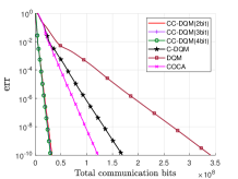
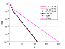
Fig. 1: Comparison with the existing ADMM-type communication-efficient algorithm.

We then compare CC-DQM with the existing first-order communication-efficient methods, including SPARQ-SGD [25] and LEAD [17]. SPARQ-SGD combines event-triggered communication with compressed communication and LEAD is a communication-compressed algorithm. For a fair comparison, in SPARQ-SGD, we use the full gradient instead of the stochastic gradient. We consider biased compressor Example 1 and the unbiased compressor Example 2. In both schemes, we let $b=2$. As shown in Fig. 2, compared with the existing first-order methods, no matter what kind of compressor is implemented, CC-DQM always enjoys the smallest communication cost. This is because CC-DQM enjoys a faster convergence rate than other algorithms.

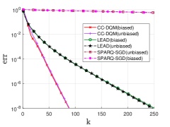
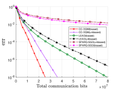
Fig. 2: Comparison with the performance of existing first-order algorithms.

Supplementary Material

Appendix A Preparation for the Proof

We first give the matrix form of CC-DQM, which is as follows:

$$\tilde{\mathbf{x}}_{k+1}={} \tilde{\mathbf{x}}_{k}-\tilde{\mathbf{D}}^{-1}\bigg{(}\nabla f(\tilde{\mathbf{x}}_{k})+\boldsymbol{\phi}_{k}+c\mathbf{L}\tilde{\mathbf{y}}_{k}\bigg{)}$$ (6a)

$$\boldsymbol{\phi}_{k+1}={} \boldsymbol{\phi}_{k}+c\mathbf{L}\tilde{\mathbf{y}}_{k+1}$$ (6b)

where $\tilde{\mathbf{D}}=2c\mathbf{D}+\nabla^{2}f(\tilde{\mathbf{y}}_{k})$. To proof Theorem 1 and Theorem 2, we introduce a key Lemma estimating the error caused by event-triggered communication and compression. Define $\tilde{\mathbf{e}}_{k}=\tilde{\mathbf{y}}_{k}-\tilde{\mathbf{x}}_{k}$.

Lemma 1.

Denote $\mathcal{C}$ as the contractive operator with the parameter $\delta\in[0,1),$ in CC-DQM, the error $\tilde{\mathbf{e}}_{k+1}$ satisfies

$$\mathbb{E}(\|\tilde{\mathbf{e}}_{k+1}\|^{2})\leq \sqrt{\delta}\mathbb{E}(\|\tilde{\mathbf{e}}_{k}\|^{2})+\frac{\delta}{1-\sqrt{\delta}}\mathbb{E}(\|\tilde{\mathbf{x}}_{k+1}-\tilde{\mathbf{x}}_{k}\|^{2})$$

$$+n\mu_{k+1}^{2}.$$ (7)

Proof.

For agent $i$ at iteration $k+1$, if $h_{i,k}=\|\mathbf{x}_{i,k+1}-\mathbf{y}_{i,k}\|-\mu_{k+1}<0$, then communication is not triggered and $\mathbf{y}_{i,k+1}=\mathbf{y}_{i,k}$. So we can get

$$\mathbf{e}_{i,k+1}=\|\mathbf{x}_{i,k+1}-\mathbf{y}_{i,k+1}\|<\mu_{k+1}$$ (8)

When $h_{i,k}>0$, $\mathbf{y}_{i,k+1}=\mathcal{C}(\mathbf{x}_{i,k+1}-\mathbf{y}_{i,k})+\mathbf{y}_{i,k}$. So we can know

$$\mathbf{e}_{i,k+1}= \mathcal{C}(\mathbf{x}_{i,k+1}-\mathbf{y}_{i,k})-(\mathbf{x}_{i,k+1}-\mathbf{y}_{i,k})$$ (9)

According to the property of compressor, we can obtain:

$$\mathbb{E}(\|\mathbf{e}_{i,k+1}\|^{2}|\mathbf{y}_{i,k},\mathbf{x}_{i,k+1})\leq{} \delta\|\mathbf{x}_{i,k+1}-\mathbf{y}_{i,k}\|^{2}$$

$$\leq{} \delta\|\mathbf{x}_{i,k+1}-\mathbf{x}_{i,k}-(\mathbf{y}_{i,k}-\mathbf{x}_{i,k})\|^{2}$$

$$\leq{} \delta(1+t^{-1})(\|\mathbf{x}_{i,k+1}-\mathbf{x}_{i,k}\|^{2})$$

$$+\delta(1+t)\|\mathbf{e}_{i,k}\|^{2}$$ (10)

Let $t=\frac{1}{\sqrt{\delta}}-1$ and take expectations, then we can obtain

$$\mathbb{E}(\|\mathbf{e}_{i,k+1}\|_{2}^{2})\leq\sqrt{\delta}\mathbb{E}(\|\mathbf{e}_{i,k}\|_{2}^{2})+\frac{\delta}{1-\sqrt{\delta}}\mathbb{E}(\|\mathbf{x}_{i,k+1}-\mathbf{x}_{i,k}\|^{2}).$$ (11)

By combing (8) and (11), then we can finish the proof. ∎

Since CC-DQM is an ADMM-type algorithm, according to [26], we give its optimal condition.

Lemma 2.

Suppose $(\tilde{\mathbf{x}}^{*},\tilde{\mathbf{z}}^{*},\boldsymbol{\lambda}^{*})$ is a primal-dual optimal pair of the augmented Larriangian. Then, it holds that $\mathbf{M}\tilde{\mathbf{x}}^{*}=\mathbf{0}$, $\frac{1}{2}\mathbf{M}_{\mathsf{u}}\tilde{\mathbf{x}}^{*}=\tilde{\mathbf{z}}^{*}$, and there exist a unique $\boldsymbol{\mu}^{*}$ lying in the column space of $\mathbf{M}$ satisfying $\boldsymbol{\phi}^{*}=\mathbf{M}^{\mathsf{T}}\boldsymbol{\mu}^{*}$, $\boldsymbol{\lambda}^{*}=[\boldsymbol{\mu}^{*};-\boldsymbol{\mu}^{*}]$, and

$$\nabla f(\tilde{\mathbf{x}}^{*})+\boldsymbol{\phi}^{*} =\mathbf{0}.$$ (12)

Next, we show the relationship between $\mathbf{r}_{k}$ and $\boldsymbol{\phi}_{k}$. As $\boldsymbol{\phi}_{0}=\boldsymbol{0}$, by recursive computation based on (6b), we have $\boldsymbol{\phi}_{k+1}=\boldsymbol{\phi}_{0}+c\sum_{s=1}^{k+1}\mathbf{L}\tilde{\mathbf{y}}_{s}=c\sum_{s=1}^{k+1}\mathbf{L}\tilde{\mathbf{y}}_{s}$. As $\mathbf{L}=\frac{1}{2}\mathbf{M}^{\mathsf{T}}\mathbf{M}$, we further have

$$\boldsymbol{\phi}_{k+1}={} 2c\mathbf{M}^{\mathsf{T}}\mathbf{r}_{k+1},$$ (13)

$$\mathbf{r}_{k+1}={} \mathbf{r}_{k}+\frac{1}{4}\mathbf{M}\tilde{\mathbf{y}}_{k+1}.$$ (14)

Recalling Lemma 2, by letting $\mathbf{r}^{*}=\frac{1}{2c}\boldsymbol{\mu}^{*}$, we have $\boldsymbol{\phi}^{*}=2c\mathbf{M}^{\mathsf{T}}\mathbf{r}^{*}$. The remain task is to show the convergence of $(\tilde{\mathbf{x}}_{k},\mathbf{r}_{k})$ to $(\tilde{\mathbf{x}}^{*},\mathbf{r}^{*})$.

Define

$$V_{k}=\frac{c}{2}\mathbb{E}(\left\|\tilde{\mathbf{x}}_{k}-\tilde{\mathbf{x}}^{*}\right\|^{2}_{\mathbf{L}_{\mathsf{u}}})+4c\mathbb{E}(\left\|\mathbf{r}_{k}-\mathbf{r}^{*}\right\|^{2})+r\mathbb{E}(\|\tilde{\mathbf{e}}_{k}\|^{2}),$$ (15)

where $r$ is a positive constant, which will be determined later. It is clear that the convergence of CC-DQM is equivalent to $V_{k}\to 0$ as $k\to\infty$. Regarding the evolution of $V_{k}$. We have the following lemma, which is infrastructural for our main result.

Lemma 3.

Under Assumptions 1, 2, 3 if $c$ and $\delta$ is chosen such that

$$\frac{\delta}{(1-\sqrt{\delta})^{2}}<\frac{G(\beta)}{3c\lambda_{n}+2c\beta\lambda_{n}+\frac{c\lambda_{n}^{2}}{\beta\lambda_{2}}},$$ (16)

with $G(\beta)>0$, $\beta>\frac{\ell^{2}}{2c\lambda_{2}v}$, where

$$G(\beta)={\frac{c\hat{\lambda}_{1}}{2}-\frac{4\ell^{2}c\beta\lambda_{2}}{4c\beta\lambda_{2}v-2\ell^{2}}-\frac{(c^{2}\hat{\lambda}_{n}^{2}+4\ell^{2})}{c\beta\lambda_{2}}},$$

then there exists $r>0$, $\eta>\frac{c\lambda_{2}}{2c\lambda_{2}v-\beta^{-1}\ell^{2}}$ and $\hat{\sigma}>0$ such that the sequence $V_{k}$ generated by CC-DQM satisfies

$$V_{k+1}\leq\frac{1}{1+\hat{\sigma}}V_{k}+n\psi\mu_{k+1}^{2},$$

where $\psi=r+\frac{1}{1+\hat{\sigma}}\left(1.5c\lambda_{n}+2c{\beta}\lambda_{n}+\frac{(c\beta^{-1}+4\hat{\sigma}c)\lambda_{n}^{2}}{2\lambda_{2}}\right)$,

$$\hat{\sigma}=\min\bigg{\{}\frac{1-\sqrt{\delta}}{\sqrt{\delta}+\frac{2c\lambda_{n}^{2}(1+\sqrt{\delta})}{r\lambda_{2}}}-\frac{\lambda_{2}(\tilde{\Xi}_{1}+\tilde{\Xi}_{2}-(1-\sqrt{\delta})\tilde{\Xi}_{1})}{\sqrt{\delta}r\lambda_{2}+2c\lambda_{n}^{2}(1+\sqrt{\delta})},$$

$$\frac{c\lambda_{2}(c\hat{\lambda}_{1}-2r\frac{\delta}{1-\sqrt{\delta}}-2\tilde{\Xi}_{1}\frac{\delta}{1-\sqrt{\delta}}-4\eta\ell^{2})-2(c^{2}\hat{\lambda}_{n}^{2}+4\ell^{2})\beta^{-1}}{8c^{2}\hat{\lambda}_{n}^{2}+32\ell^{2}+4c^{2}\lambda_{n}^{2}+4c\lambda_{2}r\frac{\delta}{1-\sqrt{\delta}}},$$

$$\frac{c\lambda_{2}(2v-\eta)-\ell^{2}\beta^{-1}}{c^{2}\lambda_{2}\hat{\lambda}_{n}+\ell^{2}}\bigg{\}}>0,$$ (17)

$$\frac{\tilde{\Xi}_{2}+\tilde{\Xi}_{1}\sqrt{\delta}}{1-\sqrt{\delta}}<r<\frac{c\hat{\lambda}_{1}-4\eta\ell^{2}}{2\frac{\delta}{1-\sqrt{\delta}}}-\frac{c^{2}\hat{\lambda}_{n}^{2}+4\ell^{2}}{c\lambda_{2}\frac{\delta}{1-\sqrt{\delta}}\beta}-\tilde{\Xi}_{1},$$

$$\tilde{\Xi}_{1}=\frac{3c\lambda_{n}}{2}+2c\beta\lambda_{n}+\frac{c\lambda_{n}^{2}}{2\beta\lambda_{2}},\qquad\tilde{\Xi}_{2}=\frac{3c\lambda_{n}}{2}+\frac{c\lambda_{n}^{2}}{2\beta\lambda_{2}}.$$

Proof.

Before proceeding, inspired by [12], we define the approximated error on $\nabla f(\tilde{\mathbf{x}}_{k+1})$ as $\boldsymbol{\delta}_{k}=\nabla f(\tilde{\mathbf{x}}_{k})+\nabla^{2}f(\tilde{\mathbf{y}}_{k})(\tilde{\mathbf{x}}_{k+1}-\tilde{\mathbf{x}}_{k})-\nabla f(\tilde{\mathbf{x}}_{k+1})$. Sine $f$ satisfies $\ell$ smooth, we can know $\|\boldsymbol{\delta}_{k}\|\leq\gamma\|\tilde{\mathbf{x}}_{k+1}-\tilde{\mathbf{x}}_{k}\|$ with $\gamma=2\ell$. Next, we begin to give our proof. Denote $\nabla^{2}f(\tilde{\mathbf{y}}_{k})$ as $\tilde{\mathbf{H}}_{k}$. According to (6a), we can obtain that

$$\nabla f(\tilde{\mathbf{x}}_{k+1})$$

$$={} \nabla f(\tilde{\mathbf{x}}_{k})+\tilde{\mathbf{H}}_{k}(\tilde{\mathbf{x}}_{k+1}-\tilde{\mathbf{x}}_{k})-\boldsymbol{\delta}_{k}$$

$$={} \tilde{\mathbf{D}}(\tilde{\mathbf{x}}_{k}-\tilde{\mathbf{x}}_{k+1})-\boldsymbol{\phi}_{k}-c\mathbf{L}\tilde{\mathbf{y}}_{k}+\tilde{\mathbf{H}}_{k}(\tilde{\mathbf{x}}_{k+1}-\tilde{\mathbf{x}}_{k})-\boldsymbol{\delta}_{k}$$

$$={} 2c\mathbf{D}(\tilde{\mathbf{x}}_{k}-\tilde{\mathbf{x}}_{k+1})-\boldsymbol{\phi}_{k}-c\mathbf{L}(\tilde{\mathbf{x}}_{k}+\tilde{\mathbf{e}}_{k})-\boldsymbol{\delta}_{k}$$

$$={} c\mathbf{L}_{\mathsf{u}}(\tilde{\mathbf{x}}_{k}-\tilde{\mathbf{x}}_{k+1})-c\mathbf{L}\tilde{\mathbf{x}}_{k+1}-\boldsymbol{\phi}_{k}-c\mathbf{L}\tilde{\mathbf{e}}_{k}-\boldsymbol{\delta}_{k}$$

$$={} c\mathbf{L}_{\mathsf{u}}(\tilde{\mathbf{x}}_{k}-\tilde{\mathbf{x}}_{k+1})-c\mathbf{L}(\tilde{\mathbf{y}}_{k+1}-\tilde{\mathbf{e}}_{k+1})-\boldsymbol{\phi}_{k}-c\mathbf{L}\tilde{\mathbf{e}}_{k}-\boldsymbol{\delta}_{k}$$

$$={} c\mathbf{L}_{\mathsf{u}}(\tilde{\mathbf{x}}_{k}-\tilde{\mathbf{x}}_{k+1})-\boldsymbol{\phi}_{k+1}+c\mathbf{L}(\tilde{\mathbf{e}}_{k+1}-\tilde{\mathbf{e}}_{k})-\boldsymbol{\delta}_{k},$$ (18)

where the third equality utilizes $\tilde{\mathbf{D}}-\tilde{\mathbf{H}}_{k}=2c\mathbf{D}$ and $\tilde{\mathbf{y}}_{k}=\tilde{\mathbf{x}}_{k}+\tilde{\mathbf{e}}_{k}$, the fourth equality utilizes $2\mathbf{D}=\mathbf{L}_{\mathsf{u}}+\mathbf{L}$. By noting that $\nabla f(\tilde{\mathbf{x}}^{*})=-\boldsymbol{\phi}^{*}$, we have

$$\mathbb{E}\big{(}(\tilde{\mathbf{x}}_{k+1}-\tilde{\mathbf{x}}^{\ast})^{\mathsf{T}}(\nabla f(\tilde{\mathbf{x}}_{k+1})-\nabla f(\tilde{\mathbf{x}}^{\ast}))\big{)}$$

$$={} \underbrace{c\mathbb{E}\big{(}(\tilde{\mathbf{x}}_{k+1}-\tilde{\mathbf{x}}^{\ast})^{\mathsf{T}}\mathbf{L}_{\mathsf{u}}(\tilde{\mathbf{x}}_{k}-\tilde{\mathbf{x}}_{k+1})}_{\Xi_{1}}\big{)}$$

$$+\underbrace{\mathbb{E}\big{(}(\tilde{\mathbf{x}}_{k+1}-\tilde{\mathbf{x}}^{\ast})^{\mathsf{T}}(\boldsymbol{\phi}^{*}-\boldsymbol{\phi}_{k+1})\big{)}}_{\Xi_{2}}+\underbrace{\mathbb{E}\big{(}(\tilde{\mathbf{x}}^{\ast}-\tilde{\mathbf{x}}_{k+1})^{\mathsf{T}}\boldsymbol{\delta}_{k}\big{)}}_{\Xi_{4}}$$

$$+\underbrace{c\mathbb{E}\big{(}(\tilde{\mathbf{x}}_{k+1}-\tilde{\mathbf{x}}^{\ast})^{\mathsf{T}}\mathbf{L}(\tilde{\mathbf{e}}_{k+1}-\tilde{\mathbf{e}}_{k})\big{)}}_{\Xi_{3}}.$$ (19)

Next, we further estimate the above four terms. Regarding $\Xi_{1}$, by using $2\mathbf{x}^{\mathsf{T}}\mathbf{A}\mathbf{y}=\|\mathbf{x}+\mathbf{y}\|_{\mathbf{A}}^{2}-\|\mathbf{x}\|_{\mathbf{A}}^{2}-\|\mathbf{y}\|_{\mathbf{A}}^{2}$, we have

$$\Xi_{1}=$$

$$\frac{c}{2}\bigg{(}\mathbb{E}(\left\|\tilde{\mathbf{x}}_{k}-\tilde{\mathbf{x}}^{*}\right\|_{\mathbf{L}_{\mathsf{u}}}^{2})-\mathbb{E}(\left\|\tilde{\mathbf{x}}_{k+1}-\tilde{\mathbf{x}}^{*}\right\|_{\mathbf{L}_{\mathsf{u}}}^{2})-\mathbb{E}(\left\|\tilde{\mathbf{x}}_{k}-\tilde{\mathbf{x}}_{k+1}\right\|_{\mathbf{L}_{\mathsf{u}}}^{2})\bigg{)}.$$

Regarding $\Xi_{2}$, as $\boldsymbol{\phi}_{k+1}-\boldsymbol{\phi}^{*}=2c\mathbf{M}^{\mathsf{T}}(\mathbf{r}_{k+1}-\mathbf{r}^{*})$, $\mathbf{M}\tilde{\mathbf{x}}^{*}=\boldsymbol{0}$, and $\mathbf{r}_{k+1}-\mathbf{r}_{k}=\frac{1}{4}\mathbf{M}\tilde{\mathbf{y}}_{k+1}$, one has

$$\Xi_{2}={} -2c\mathbb{E}\big{(}\tilde{\mathbf{x}}_{k+1}^{\mathsf{T}}\mathbf{M}^{\mathsf{T}}(\mathbf{r}_{k+1}-\mathbf{r}^{*})\big{)}$$

$$={} -2c\mathbb{E}\big{(}(\tilde{\mathbf{y}}_{k+1}-\tilde{\mathbf{e}}_{k+1})^{\mathsf{T}}\mathbf{M}^{\mathsf{T}}(\mathbf{r}_{k+1}-\mathbf{r}^{*})\big{)}$$

$$={} 4c\mathbb{E}\bigg{(}\left\|\mathbf{r}_{k}-\mathbf{r}^{*}\right\|^{2}-\left\|\mathbf{r}_{k+1}-\mathbf{r}^{*}\right\|^{2}-\left\|\mathbf{r}_{k}-\mathbf{r}_{k+1}\right\|^{2}\bigg{)}$$

$$+2c\mathbb{E}\big{(}\tilde{\mathbf{e}}_{k+1}^{\mathsf{T}}\mathbf{M}^{\mathsf{T}}(\mathbf{r}_{k+1}-\mathbf{r}^{*})\big{)}$$

$$\leq{} 4c\mathbb{E}\bigg{(}\left\|\mathbf{r}_{k}-\mathbf{r}^{*}\right\|^{2}-\left\|\mathbf{r}_{k+1}-\mathbf{r}^{*}\right\|^{2}-\left\|\mathbf{r}_{k}-\mathbf{r}_{k+1}\right\|^{2}\bigg{)}$$

$$+2c\beta\mathbb{E}(\tilde{\mathbf{e}}_{k+1}^{\mathsf{T}}\mathbf{L}\tilde{\mathbf{e}}_{k+1})+c\beta^{-1}\mathbb{E}(\left\|\mathbf{r}_{k+1}-\mathbf{r}^{*}\right\|^{2}).$$

Regarding $\Xi_{3}$, we have

$$\Xi_{3}={} \frac{c}{2}\mathbb{E}\big{(}\tilde{\mathbf{x}}_{k+1}^{\mathsf{T}}\mathbf{M}^{\mathsf{T}}\mathbf{M}(\tilde{\mathbf{e}}_{k+1}-\tilde{\mathbf{e}}_{k})\big{)}$$

$$={} \frac{c}{2}\mathbb{E}\big{(}(\tilde{\mathbf{y}}_{k+1}-\tilde{\mathbf{e}}_{k+1})^{\mathsf{T}}\mathbf{M}^{\mathsf{T}}\mathbf{M}(\tilde{\mathbf{e}}_{k+1}-\tilde{\mathbf{e}}_{k})\big{)}$$

$$={} 2c\mathbb{E}\big{(}(\mathbf{r}_{k+1}-\mathbf{r}_{k})^{\mathsf{T}}\mathbf{M}(\tilde{\mathbf{e}}_{k+1}-\tilde{\mathbf{e}}_{k})\big{)}+c\mathbb{E}\big{(}\tilde{\mathbf{e}}_{k+1}^{\mathsf{T}}\mathbf{L}(\tilde{\mathbf{e}}_{k}-\tilde{\mathbf{e}}_{k+1})\big{)}$$

$$\leq{} \frac{c}{2}\mathbb{E}\big{(}(\tilde{\mathbf{e}}_{k+1}-\tilde{\mathbf{e}}_{k})^{\mathsf{T}}\mathbf{L}(\tilde{\mathbf{e}}_{k+1}-\tilde{\mathbf{e}}_{k})\big{)}+4c\mathbb{E}\big{(}\left\|\mathbf{r}_{k+1}-\mathbf{r}_{k}\right\|^{2}\big{)}$$

$$+c\mathbb{E}\big{(}\tilde{\mathbf{e}}^{\mathsf{T}}_{k+1}\mathbf{L}\tilde{\mathbf{e}}_{k}\big{)}.$$

Regarding $\Xi_{4}$, we have

$$\Xi_{4} \leq{}\frac{\eta}{2}\mathbb{E}(\left\|\boldsymbol{\delta}_{k}\right\|^{2})+\frac{1}{2\eta}\mathbb{E}(\left\|\tilde{\mathbf{x}}_{k+1}-\tilde{\mathbf{x}}^{*}\right\|^{2})$$

$$\leq{}\frac{\eta\gamma^{2}}{2}\mathbb{E}(\left\|\tilde{\mathbf{x}}_{k+1}-\tilde{\mathbf{x}}_{k}\right\|^{2})+\frac{1}{2\eta}\mathbb{E}(\left\|\tilde{\mathbf{x}}_{k+1}-\tilde{\mathbf{x}}^{*}\right\|^{2}).$$

Define

$$\tilde{V}_{k}=\frac{c}{2}\mathbb{E}(\left\|\tilde{\mathbf{x}}_{k}-\tilde{\mathbf{x}}^{*}\right\|^{2}_{\mathbf{L}_{\mathsf{u}}})+4c\mathbb{E}(\left\|\mathbf{r}_{k}-\mathbf{r}^{*}\right\|^{2}).$$

Due to the $v$-strongly convexity of $f$, we have $(\tilde{\mathbf{x}}_{k+1}-\tilde{\mathbf{x}}^{\ast})^{\mathsf{T}}(\nabla f(\tilde{\mathbf{x}}_{k+1})-\nabla f(\tilde{\mathbf{x}}^{\ast}))\geq v\left\|\tilde{\mathbf{x}}_{k+1}-\tilde{\mathbf{x}}^{*}\right\|^{2}$, which yields

$$v\mathbb{E}(\left\|\tilde{\mathbf{x}}_{k+1}-\tilde{\mathbf{x}}^{*}\right\|^{2})$$

$$\leq{} \Xi_{1}+\Xi_{2}+\Xi_{3}+\Xi_{4}$$

$$\leq{} \tilde{V}_{k}-\tilde{V}_{k+1}+\bigg{(}\frac{\eta\gamma^{2}}{2}-\frac{c\hat{\lambda}_{1}}{2}\bigg{)}\mathbb{E}(\left\|\tilde{\mathbf{x}}_{k+1}-\tilde{\mathbf{x}}_{k}\right\|^{2})$$

$$+c\beta^{-1}\mathbb{E}(\left\|\mathbf{r}_{k+1}-\mathbf{r}^{*}\right\|^{2})+{c\lambda_{n}(2\beta+1)}\mathbb{E}(\left\|\tilde{\mathbf{e}}_{k+1}\right\|^{2})$$

$$+{c\lambda_{n}}\mathbb{E}(\left\|\tilde{\mathbf{e}}_{k}\right\|^{2})+c\lambda_{n}\mathbb{E}(\|\tilde{\mathbf{e}}_{k}\|\|\tilde{\mathbf{e}}_{k+1}\|)+\frac{1}{2\eta}\mathbb{E}(\left\|\tilde{\mathbf{x}}_{k+1}-\tilde{\mathbf{x}}^{*}\right\|^{2})$$

$$\leq{} \tilde{V}_{k}-(1+\hat{\sigma})\tilde{V}_{k+1}+\bigg{(}\frac{\eta\gamma^{2}}{2}-\frac{c\hat{\lambda}_{1}}{2}\bigg{)}\mathbb{E}(\left\|\tilde{\mathbf{x}}_{k+1}-\tilde{\mathbf{x}}_{k}\right\|^{2})$$

$$+\bigg{(}\frac{1}{2\eta}+\frac{c\hat{\sigma}\hat{\lambda}_{n}}{2}\bigg{)}\mathbb{E}(\left\|\tilde{\mathbf{x}}_{k+1}-\tilde{\mathbf{x}}^{*}\right\|^{2})$$

$$+\bigg{(}c\beta^{-1}+4c\hat{\sigma}\bigg{)}\mathbb{E}(\left\|\mathbf{r}_{k+1}-\mathbf{r}^{*}\right\|^{2})$$

$$+\frac{c\lambda_{n}(4\beta+3)}{2}\mathbb{E}\bigg{(}\left\|\tilde{\mathbf{e}}_{k+1}\right\|^{2})+\left\|\tilde{\mathbf{e}}_{k}\right\|^{2}\bigg{)}.$$ (20)

Next, we consider the term $\left\|\mathbf{r}_{k+1}-\mathbf{r}^{*}\right\|^{2}$. Recalling (18), we have

$$\nabla f(\tilde{\mathbf{x}}_{k+1})-\nabla f(\tilde{\mathbf{x}}^{*})+c\mathbf{L}_{\mathsf{u}}(\tilde{\mathbf{x}}_{k+1}-\tilde{\mathbf{x}}_{k})+\boldsymbol{\delta}_{k}$$

$$={} c\mathbf{L}(\tilde{\mathbf{e}}_{k+1}-\tilde{\mathbf{e}}_{k})-2c\mathbf{M}^{\mathsf{T}}(\mathbf{r}_{k+1}-\mathbf{r}^{*})$$ (21)

Denote the left-side and right-side of equation (21) as $\Xi_{L}$ and $\Xi_{R}$, respectively. By applying $\|\mathbf{x}+\mathbf{y}\|^{2}\geq\frac{1}{2}\|\mathbf{y}\|^{2}-\|\mathbf{x}\|^{2}$ to $\left\|\Xi_{R}\right\|^{2}$, we obtain

$$\left\|\Xi_{R}\right\|^{2}\geq{} \frac{1}{2}\left\|2c\mathbf{M}^{\mathsf{T}}(\mathbf{r}_{k+1}-\mathbf{r}^{\ast})\right\|^{2}-c^{2}\left\|\mathbf{L}(\mathbf{e}_{k+1}-\mathbf{e}_{k})\right\|^{2}$$

$$\geq{} 4c^{2}\lambda_{2}\|\mathbf{r}_{k+1}-\mathbf{r}^{\ast}\|^{2}-2c^{2}\lambda_{n}^{2}(\left\|\mathbf{e}_{k}\right\|^{2}+\left\|\mathbf{e}_{k+1}\right\|^{2}).$$

Regarding $\left\|\Xi_{L}\right\|^{2}$, we have

$$\left\|\Xi_{L}\right\|^{2}\leq{} 2\ell^{2}\|\tilde{\mathbf{x}}_{k+1}-\tilde{\mathbf{x}}^{\ast}\|^{2}+4\Big{(}c^{2}\hat{\lambda}_{n}^{2}+\gamma^{2}\Big{)}\|\tilde{\mathbf{x}}_{k+1}-\tilde{\mathbf{x}}_{k}\|^{2}.$$

Combining estimation on $\left\|\Xi_{R}\right\|^{2}$ and $\left\|\Xi_{L}\right\|^{2}$ yields

$$\mathbb{E}(\left\|\mathbf{r}_{k+1}-\mathbf{r}^{*}\right\|^{2})\leq{} \frac{c^{2}\hat{\lambda}_{n}^{2}+\gamma^{2}}{c^{2}\lambda_{2}}\mathbb{E}(\|\tilde{\mathbf{x}}_{k+1}-\tilde{\mathbf{x}}_{k}\|^{2})$$

$$+\frac{\lambda_{n}^{2}}{2\lambda_{2}}\mathbb{E}((\left\|\tilde{\mathbf{e}}_{k}\right\|^{2}+\left\|\tilde{\mathbf{e}}_{k+1}\right\|^{2}))$$

$$+\frac{\ell^{2}}{2c^{2}\lambda_{2}}\mathbb{E}(\|\tilde{\mathbf{x}}_{k+1}-\mathbf{x}^{\ast}\|^{2}).$$ (22)

Substituting (22) into (20), we have

$$(1+\hat{\sigma})\tilde{V}_{k+1}-\tilde{V}_{k}$$

$$\leq{} \bigg{(}\frac{(\beta^{-1}+4\hat{\sigma})(c^{2}\hat{\lambda}_{n}^{2}+\gamma^{2})}{c\lambda_{2}}-\frac{c\hat{\lambda}_{1}-\eta\gamma^{2}}{2}\bigg{)}\mathbb{E}(\left\|\tilde{\mathbf{x}}_{k+1}-\tilde{\mathbf{x}}_{k}\right\|^{2})$$

$$+\bigg{(}\frac{1}{2\eta}+\frac{c\hat{\sigma}\hat{\lambda}_{n}}{2}+\frac{\ell^{2}(\beta^{-1}+4\hat{\sigma})}{2c\lambda_{2}}-v\bigg{)}\mathbb{E}(\left\|\tilde{\mathbf{x}}_{k+1}-\tilde{\mathbf{x}}^{*}\right\|^{2})$$

$$+\underbrace{\big{(}2\beta c\lambda_{n}+\frac{3c\lambda_{n}}{2}+\frac{(1+4\hat{\sigma}\beta)c\lambda_{n}^{2}}{2\lambda_{2}\beta})}_{\Xi_{1}}\mathbb{E}(\|\tilde{\mathbf{e}}_{k+1}\|^{2})$$

$$+\underbrace{\bigg{(}\frac{3c\lambda_{n}}{2}+\frac{(1+4\hat{\sigma}\beta)c\lambda_{n}^{2}}{2\lambda_{2}\beta}\bigg{)}}_{\Xi_{2}}\mathbb{E}(\left\|\tilde{\mathbf{e}}_{k}\right\|^{2}).$$ (23)

According to the definition of $V_{k}$, we can know

$$V_{k}-(1+\hat{\sigma})V_{k+1}= \tilde{V}_{k}+r\mathbb{E}(\|\tilde{\mathbf{e}}_{k}\|^{2})-(1+\hat{\sigma})\tilde{V}_{k+1}$$

$$-(1+\hat{\sigma})r\mathbb{E}(\|\tilde{\mathbf{e}}_{k+1}\|^{2}).$$ (24)

In Lemma 1, the relationship between $\mathbb{E}(\|\tilde{\mathbf{e}}_{k+1}\|^{2})$ and $\mathbb{E}(\|\tilde{\mathbf{e}}_{k}\|^{2})$ is estimated, which can be seen in (7). To estimate $V_{k}$, we substitute (7) and (23) into (24), thus obtaining

$$(1+\hat{\sigma}){V}_{k+1}-{V}_{k}$$

$$\leq{}\bigg{(} -\frac{c\hat{\lambda}_{1}-\eta\gamma^{2}}{2}+\frac{(\beta^{-1}+4\hat{\sigma})(c^{2}\hat{\lambda}_{n}^{2}+\gamma^{2})}{c\lambda_{2}}$$

$$+\frac{r(1+\hat{\sigma})\delta}{1-\sqrt{\delta}}+\Xi_{1}\frac{\delta}{1-\sqrt{\delta}}\bigg{)}\mathbb{E}(\left\|\tilde{\mathbf{x}}_{k+1}-\tilde{\mathbf{x}}_{k}\right\|^{2})$$

$$+\bigg{(}\frac{1}{2\eta}+\frac{c\hat{\sigma}\hat{\lambda}_{n}}{2}+\frac{\ell^{2}(\beta^{-1}+4\hat{\sigma})}{2c\lambda_{2}}-v\bigg{)}\mathbb{E}(\left\|\tilde{\mathbf{x}}_{k+1}-\tilde{\mathbf{x}}^{*}\right\|^{2})$$

$$+\bigg{(}r(1+\hat{\sigma})\sqrt{\delta}+\Xi_{1}\sqrt{\delta}-r+\Xi_{2}\bigg{)}\mathbb{E}(\left\|\tilde{\mathbf{e}}_{k}\right\|^{2})$$

$$+\bigg{(}r(1+\hat{\sigma})+\Xi_{1}\bigg{)}n\mu_{k+1}^{2}.$$ (25)

To obtain the result, the coefficients associated with the $\mathbb{E}(\|\tilde{\mathbf{x}}_{k+1}\|^{2})$, $\mathbb{E}(\|\tilde{\mathbf{x}}_{k}\|^{2})$ and $\mathbb{E}(\|\tilde{\mathbf{e}}_{k+1}\|^{2})$ in (25) are required to be negative. That is

$$r-\Xi_{2}-\Xi_{1}\sqrt{\delta}-(1+\hat{\sigma})r\sqrt{\delta} \geq 0{},$$

$$v-\frac{1}{2\eta}-\frac{\hat{\sigma}c\hat{\lambda}_{n}}{2}-\frac{\ell^{2}(\beta^{-1}+4\hat{\sigma})}{2c\lambda_{2}}\geq{}0,$$

$$\frac{c\hat{\lambda}_{1}-\eta\gamma^{2}}{2}-\frac{(r+\Xi_{1})\delta}{1-\sqrt{\delta}}-\frac{r\delta\hat{\sigma}}{1-\sqrt{\delta}}$$

$$-\frac{(c^{2}\hat{\lambda}_{n}^{2}+\gamma^{2})(\beta^{-1}+4\hat{\sigma})}{c\lambda_{2}}\geq{}0.$$

Define

$$\tilde{\Xi}_{1}=\Xi_{1}|_{\hat{\sigma}=0}=\frac{3c\lambda_{n}}{2}+{2c\beta\lambda_{n}}+\frac{c\beta^{-1}\lambda_{n}^{2}}{2\lambda_{2}},$$

$$\tilde{\Xi}_{2}=\Xi_{2}|_{\hat{\sigma}=0}=\frac{3c\lambda_{n}}{2}+\frac{c\beta^{-1}\lambda_{n}^{2}}{2\lambda_{2}}.$$

As $\hat{\sigma}$ can be chosen as a sufficiently small positive real number, it suffice to require

$$r-\tilde{\Xi}_{2}-\tilde{\Xi}_{1}\sqrt{\delta}-r\sqrt{\delta}>0{},$$ (26)

$$\frac{c\hat{\lambda}_{1}-\eta\gamma^{2}}{2}-\frac{(r+\tilde{\Xi}_{1})\delta}{1-\sqrt{\delta}}-\frac{(c^{2}\hat{\lambda}_{n}^{2}+\gamma^{2})\beta^{-1}}{c\lambda_{2}}>{}0,$$ (27)

$$v-\frac{1}{2\eta}-\frac{\ell^{2}\beta^{-1}}{2c\lambda_{2}}>{}0\Rightarrow\eta>\frac{c\lambda_{2}}{2c\lambda_{2}v-\beta^{-1}\ell^{2}}.$$

Regarding (26), we can get

$$r>\frac{\tilde{\Xi}_{2}+\tilde{\Xi}_{1}\sqrt{\delta}}{1-\sqrt{\delta}}.$$

To ensure (27) can be satisfied, in (27), let $r=\frac{\tilde{\Xi}_{2}+\tilde{\Xi}_{1}\sqrt{\delta}}{1-\sqrt{\delta}}$ and $\eta=\frac{c\lambda_{2}}{2c\lambda_{2}v-\beta^{-1}\ell^{2}}$, then we can obtain

$$\frac{c\hat{\lambda}_{1}}{2}-\frac{(\tilde{\Xi}_{1}+\tilde{\Xi}_{2})\delta}{(1-\sqrt{\delta})^{2}}-\frac{c\lambda_{2}\gamma^{2}}{4c\lambda_{2}v-2\beta^{-1}\ell^{2}}-\frac{(c^{2}\hat{\lambda}_{n}^{2}+\gamma^{2})}{c\beta\lambda_{2}}>0$$ (28)

Rearrange the terms, then we can obtain:

$$\frac{\delta}{(1-\sqrt{\delta})^{2}}<\frac{\frac{c\hat{\lambda}_{1}}{2}-\frac{c\lambda_{2}\gamma^{2}\beta}{4c\beta\lambda_{2}v-2\ell^{2}}-\frac{(c^{2}\hat{\lambda}_{n}^{2}+\gamma^{2})}{c\beta\lambda_{2}}}{3c\lambda_{n}+2c\beta\lambda_{n}+\frac{c\lambda_{n}^{2}}{\beta\lambda_{2}}}$$ (29)

Define the RHS of (29) as

$$F(c,\beta)=\frac{\frac{\hat{\lambda}_{1}}{2}-\frac{\lambda_{2}\gamma^{2}\beta}{4c\beta\lambda_{2}v-2\ell^{2}}-\frac{(c^{2}\hat{\lambda}_{n}^{2}+\gamma^{2})}{c^{2}\beta\lambda_{2}}}{3\lambda_{n}+2\beta\lambda_{n}+\frac{\lambda_{n}^{2}}{\beta\lambda_{2}}}.$$

It is easy to obtain

$$F(c,\beta)<F(\infty,\beta)=\frac{\frac{\hat{\lambda}_{1}}{2}-\frac{\hat{\lambda}_{n}^{2}}{\beta\lambda_{2}}}{3\lambda_{n}+2\beta\lambda_{n}+\frac{\lambda_{n}^{2}}{\beta\lambda_{2}}}.$$

We find that $F(\infty,\beta)$ has a global maximum when $\beta=\beta^{*}=2u+\sqrt{4u^{2}+\frac{1}{2}\frac{\lambda_{n}}{\lambda_{2}}+3u}$, where $u=\frac{\hat{\lambda}_{n}^{2}}{\lambda_{2}\hat{\lambda}_{1}}$. So when $\delta$ is chosen such that $\frac{\delta}{(1-\sqrt{\delta})^{2}}<F(\infty,\beta^{*})$, then there always exist a sufficient large $c$ which can ensure that (29) is satisfied. ∎

Appendix B Proof of Theorem 1 and Theorem 2

Proof.

According to Lemma (3), we can know

$$V_{k+1}\leq\frac{1}{1+\hat{\sigma}}V_{k}+n\psi\mu_{k+1}^{2},\text{with}$$

$$\psi=r+\frac{1}{1+\hat{\sigma}}\left(1.5c\lambda_{n}+2c{\beta}\lambda_{n}+\frac{(c\beta^{-1}+4\hat{\sigma}c)\lambda_{n}^{2}}{2\lambda_{2}}\right).$$

When $\mu_{k}=0$, then we can obtain:

$$V_{k+1}\leq\frac{1}{1+\hat{\sigma}}V_{k}\leq\frac{1}{(1+\hat{\sigma})^{2}}V_{k-1}\dots\leq\frac{V_{0}}{(1+\hat{\sigma})^{k+1}}.$$ (30)

Define $\sigma=\frac{1}{1+\hat{\sigma}}$, then the proof of Theorem 1 is completed.

When $\mu_{k}=\alpha\rho^{k-1}$, we can get obtain

$$V_{k+1} \leq\frac{V_{k}}{1+\hat{\sigma}}+n\psi\alpha\mu_{k+1}^{2}$$ (31)

$$\leq\frac{V_{k-1}}{(1+\hat{\sigma})^{2}}+\frac{n\psi\alpha\mu_{k}^{2}}{1+\hat{\sigma}}+n\psi\alpha\mu_{k+1}^{2}\leq\dots$$

$$\leq V_{0}\sigma^{k+1}+\sum_{t=0}^{k}{n\psi\alpha\rho^{2(k-t)}}\sigma^{t}$$

$${}=\sigma^{k+1}\big{(}V_{0}+n\psi\alpha\sigma^{-1}\sum_{t=0}^{k-1}(\frac{\rho^{2}}{\sigma})^{t}\big{)}$$ (32)

Let $\tilde{\sigma}=\max(\sigma,\rho^{2})$, according to (32), when $\tilde{\sigma}\neq\rho^{2}$, we can know

$$V_{k+1}\leq \tilde{\sigma}^{k+1}\big{(}V_{0}+n\psi\alpha\tilde{\sigma}^{-1})\sum_{t=0}^{k}(\frac{\rho^{2}}{\tilde{\sigma}})^{t}\big{)}$$

$$\leq \tilde{\sigma}^{k+1}\big{(}V_{0}+n\psi\alpha\tilde{\sigma}^{-1})\frac{\tilde{\sigma}}{\tilde{\sigma}-\rho^{2}}.$$ (33)

When $\tilde{\sigma}=\rho^{2}$, we can get $V_{k+1}\leq k\tilde{\sigma}^{k+1}(V_{0}+n\psi\alpha\tilde{\sigma}^{-1})$. ∎

Appendix C Proof of Corollary 1

Proof.

Revisiting (19), since the compressor is unbiased, then we can obtain

$$\Xi_{3}={} c\mathbb{E}\big{(}(\tilde{\mathbf{x}}_{k+1}-\tilde{\mathbf{x}}^{\ast})^{\mathsf{T}}\mathbf{L}(\tilde{\mathbf{e}}_{k+1}-\tilde{\mathbf{e}}_{k})\big{)}=-c\mathbb{E}(\tilde{\mathbf{e}}_{k}^{\mathsf{T}}\mathbf{L}\tilde{\mathbf{x}}_{k+1}),$$

$$={} c\mathbb{E}\big{(}(\tilde{\mathbf{y}}_{k+1}-\tilde{\mathbf{e}}_{k+1})^{\mathsf{T}}\mathbf{L}\tilde{\mathbf{e}}_{k}\big{)}=c\mathbb{E}\big{(}(\tilde{\mathbf{y}}_{k+1})^{\mathsf{T}}\mathbf{L}\tilde{\mathbf{e}}_{k}\big{)}$$

$$={} 2c\mathbb{E}\big{(}(\mathbf{r}_{k+1}-\mathbf{r}_{k})^{\mathsf{T}}\mathbf{M}\tilde{\mathbf{e}}_{k}\big{)},$$

$$\leq{} 4c\mathbb{E}(\|\mathbf{r}_{k+1}-\mathbf{r}_{k}\|^{2})+\frac{c\lambda_{n}}{2}\mathbb{E}(\|\tilde{\mathbf{e}}_{k}\|^{2})$$

$$\Xi_{2}={} -2c\mathbb{E}\big{(}\tilde{\mathbf{x}}_{k+1}^{\mathsf{T}}\mathbf{M}^{\mathsf{T}}(\mathbf{r}_{k+1}-\mathbf{r}^{*})\big{)}$$

$$={} -2c\mathbb{E}\big{(}(\tilde{\mathbf{y}}_{k+1}-\tilde{\mathbf{e}}_{k+1})^{\mathsf{T}}\mathbf{M}^{\mathsf{T}}(\mathbf{r}_{k+1}-\mathbf{r}^{*})\big{)}$$

$$={} 4c\mathbb{E}\bigg{(}\left\|\mathbf{r}_{k}-\mathbf{r}^{*}\right\|^{2}-\left\|\mathbf{r}_{k+1}-\mathbf{r}^{*}\right\|^{2}-\left\|\mathbf{r}_{k}-\mathbf{r}_{k+1}\right\|^{2}\bigg{)}$$

$$+c\mathbb{E}(\|\tilde{\mathbf{e}}_{k+1}\|_{\mathbf{L}}^{2})$$

$$\leq{} 4c\mathbb{E}\bigg{(}\left\|\mathbf{r}_{k}-\mathbf{r}^{*}\right\|^{2}-\left\|\mathbf{r}_{k+1}-\mathbf{r}^{*}\right\|^{2}-\left\|\mathbf{r}_{k}-\mathbf{r}_{k+1}\right\|^{2}\bigg{)}$$

$$+{}c\lambda_{n}\mathbb{E}(\|\tilde{\mathbf{e}}_{k+1}\|^{2}).$$

By reusing the strong convexity of $f$ as (20), we can know:

$$v\mathbb{E}(\left\|\tilde{\mathbf{x}}_{k+1}-\tilde{\mathbf{x}}^{*}\right\|^{2})$$

$$\leq{} \Xi_{1}+\Xi_{2}+\Xi_{3}+\Xi_{4}$$

$$\leq{} \tilde{V}_{k}-\tilde{V}_{k+1}+\bigg{(}\frac{\eta\gamma^{2}}{2}-\frac{c\hat{\lambda}_{1}}{2}\bigg{)}\mathbb{E}(\left\|\tilde{\mathbf{x}}_{k+1}-\tilde{\mathbf{x}}_{k}\right\|^{2})$$

$$+\frac{1}{2\eta}\mathbb{E}(\left\|\tilde{\mathbf{x}}_{k+1}-\tilde{\mathbf{x}}^{*}\right\|^{2})$$ (34)

According to the definition of $V_{k+1}$, we can obtain:

$$\tilde{V}_{k}-\tilde{V}_{k+1}$$

$$={} V_{k}-(1+\sigma)V_{k+1}+\frac{c\sigma\hat{\lambda}_{n}}{2}\mathbb{E}(\|\tilde{\mathbf{x}}_{k+1}-\tilde{\mathbf{x}}^{*}\|^{2})$$

$$-r\mathbb{E}(\|\tilde{\mathbf{e}}_{k}\|^{2})+4c\sigma\mathbb{E}{\|\mathbf{r}_{k+1}-\mathbf{r}^{*}\|^{2}}+(1+\sigma)r\mathbb{E}(\|\tilde{\mathbf{e}}_{k+1}\|^{2})$$

$$\leq V_{k}-(1+\sigma)V_{k+1}+\frac{c\sigma}{2}\hat{\lambda}_{n}\mathbb{E}(\|\tilde{\mathbf{x}}_{k+1}-\tilde{\mathbf{x}}^{*}\|^{2})$$

$$+\frac{(1+\sigma)r\delta}{1-\sqrt{\delta}}\mathbb{E}(\|\tilde{\mathbf{x}}_{k+1}-\tilde{\mathbf{x}}_{k}\|^{2})+r\big{(}(1+\sigma)\sqrt{\delta}-1\big{)}\mathbb{E}(\|\tilde{\mathbf{e}}_{k}\|^{2})$$

$$+4c\sigma\mathbb{E}{\|\mathbf{r}_{k+1}-\mathbf{r}^{*}\|^{2}}$$

$$\overset{\eqref{eq:rk-rstar-bound}}{\leq} V_{k}-(1+\sigma)V_{k+1}+(\frac{c\sigma\hat{\lambda}_{n}}{2}+\frac{2\ell^{2}\sigma}{c\lambda_{2}})\mathbb{E}(\|\tilde{\mathbf{x}}_{k+1}-\tilde{\mathbf{x}}^{*}\|^{2})$$

$$+\left.\bigg{(}\frac{4c^{2}\sigma\hat{\lambda}_{n}^{2}}{c\lambda_{2}}+\frac{4\sigma\gamma^{2}}{c\lambda_{2}}+\frac{2\delta\lambda_{n}^{2}c\sigma}{(1-\sqrt{\delta})\lambda_{2}}+\frac{(1+\sigma)r\delta}{(1-\sqrt{\delta})}\right.$$

$$\left.+\frac{\delta c\lambda_{n}}{1-\sqrt{\delta}}\right.\bigg{)}\mathbb{E}(\|\tilde{\mathbf{x}}_{k+1}-\tilde{\mathbf{x}}_{k}\|^{2})+\big{(}r(1+\sigma)\sqrt{\delta}-r\big{)}\mathbb{E}(\|\tilde{\mathbf{e}}_{k}\|^{2})$$

$$+\frac{2\lambda_{n}^{2}c\sigma(1+\sqrt{\delta})}{\lambda_{2}}\mathbb{E}(\|\tilde{\mathbf{e}}_{k}\|^{2})+(\sqrt{\delta}c\lambda_{n}+\frac{c\lambda_{n}}{2})\mathbb{E}(\|\tilde{\mathbf{e}}_{k}\|^{2})$$ (35)

Substitute (35) into (34) and rearrange the terms, then we can get:

$$V_{k}-(1+\sigma)V_{k+1}$$

$$\geq \bigg{(}\frac{c\hat{\lambda}_{1}}{2}-\frac{\eta\gamma^{2}}{2}-\frac{2\delta\lambda_{n}^{2}c\sigma}{(1-\sqrt{\delta})\lambda_{2}}-\frac{4c^{2}\sigma\hat{\lambda}_{n}^{2}+4\sigma\gamma^{2}}{c\lambda_{2}}$$

$$\left.-\frac{(1+\sigma)r\delta}{1-\sqrt{\delta}}-\frac{\delta c\lambda_{n}}{1-\sqrt{\delta}}\bigg{)}\right.\mathbb{E}(\|\tilde{\mathbf{x}}_{k+1}-\tilde{\mathbf{x}}_{k}\|^{2})$$

$$+\bigg{(}r-r(1+\sigma)\sqrt{\delta}-\frac{2\lambda_{n}^{2}c\sigma(1+\sqrt{\delta})}{\lambda_{2}}$$

$$-\sqrt{\delta}c\lambda_{n}-\frac{c\lambda_{n}}{2}\bigg{)}\mathbb{E}(\|\tilde{\mathbf{e}}_{k}\|^{2})$$

$$+\bigg{(}v-\frac{c\sigma\hat{\lambda}_{n}}{2}-\frac{2\ell^{2}\sigma}{c\lambda_{2}}-\frac{1}{2\eta}\bigg{)}\mathbb{E}(\|\tilde{\mathbf{x}}_{k+1}-\tilde{\mathbf{x}}^{*}\|^{2})$$ (36)

To ensure the linear convergence of $V_{k}$, let the RHS of (36) be greater than $0$, that is, the coefficient of each term should always be positive, which yields

$$v-\frac{c\sigma\hat{\lambda}_{n}}{2}-\frac{2\ell^{2}\sigma}{c\lambda_{2}}-\frac{1}{2\eta}\geq 0,$$ (37)

$$r-r(1+\sigma)\sqrt{\delta}-\frac{2\lambda_{n}^{2}c\sigma(1+\sqrt{\delta})}{\lambda_{2}}-\sqrt{\delta}c\lambda_{n}-\frac{c\lambda_{n}}{2}\geq 0$$

$$\frac{c\hat{\lambda}_{1}}{2}-\frac{\eta\gamma^{2}}{2}-\frac{2\delta\lambda_{n}^{2}c\sigma}{(1-\sqrt{\delta})\lambda_{2}}-\frac{4c^{2}\sigma\hat{\lambda}_{n}^{2}+4\sigma\gamma^{2}}{c\lambda_{2}},$$

$$-\frac{(1+\sigma)r\delta}{1-\sqrt{\delta}}-\frac{\delta c\lambda_{n}}{1-\sqrt{\delta}}\geq 0$$ (38)

Since $\sigma>0$ can be arbitrary small, to satisfied (38), we need

$$r(1-\sqrt{\delta})\geq\sqrt{\delta}c\lambda_{n}+\frac{c\lambda_{n}}{2}\Rightarrow r\geq\frac{\sqrt{\delta}c\lambda_{n}+\frac{c\lambda_{n}}{2}}{1-\sqrt{\delta}},$$

$$v-\frac{1}{2\eta}\geq 0\Rightarrow\eta\geq\frac{1}{2v},$$

$$\frac{c\hat{\lambda_{1}}}{2}-\frac{\eta\gamma^{2}}{2}-\frac{r\delta}{1-\sqrt{\delta}}-\frac{\delta c\lambda_{n}}{1-\sqrt{\delta}}\geq 0.$$ (39)

Rearrange (C), we can get

$$c\big{(}\frac{\hat{\lambda}_{1}}{2}-\frac{3\lambda_{n}}{2}\frac{\delta}{(1-\sqrt{\delta})^{2}}\big{)}>\frac{\gamma^{2}}{4v}.$$ (40)

Since $c>0$ and $\gamma=2\ell$, to make sure the existence of $c$, let $\frac{\hat{\lambda}_{1}}{2}-\frac{3\lambda_{n}}{2}\frac{\delta}{(1-\sqrt{\delta})^{2}}>0$, then we can obtain

$$c>\frac{\ell^{2}}{v}\frac{2(1-\sqrt{\delta})^{2}}{\hat{\lambda}_{1}(1-\sqrt{\delta})^{2}-3\lambda_{n}\delta}$$ (41)

When $\delta=0$, (41) becomes $c>\frac{2\ell^{2}}{v\hat{\lambda}_{1}}$, which is the requirement of the penalty parameter c in DQM [12]. ∎

References

• [1] Yongcan Cao, Wenwu Yu, Wei Ren, and Guanrong Chen, “An overview of recent progress in the study of distributed multi-agent coordination,” IEEE Transactions on Industrial Informatics, vol. 9, no. 1, pp. 427–438, 2013.
• [2] Hao Jan Liu, Wei Shi, and Hao Zhu, “Distributed voltage control in distribution networks: Online and robust implementations,” IEEE Transactions on Smart Grid, vol. 9, no. 6, pp. 6106–6117, 2018.
• [3] Joel B. Predd, Sanjeev R. Kulkarni, and H. Vincent Poor, “A collaborative training algorithm for distributed learning,” IEEE Transactions on Information Theory, vol. 55, no. 4, pp. 1856–1871, 2009.
• [4] Usman A. Khan, Soummya Kar, and José M. F. Moura, “Diland: An algorithm for distributed sensor localization with noisy distance measurements,” IEEE Transactions on Signal Processing, vol. 58, no. 3, pp. 1940–1947, 2010.
• [5] Angelia Nedic and Asuman Ozdaglar, “Distributed subgradient methods for multi-agent optimization,” IEEE Transactions on Automatic Control, vol. 54, no. 1, pp. 48–61, 2009.
• [6] Wei Shi, Qing Ling, Gang Wu, and Wotao Yin, “EXTRA: An exact first-order algorithm for decentralized consensus optimization,” SIAM Journal on Optimization, vol. 25, no. 2, pp. 944–966, 2015.
• [7] Guannan Qu and Na Li, “Harnessing smoothness to accelerate distributed optimization,” IEEE Transactions on Control of Network Systems, vol. 5, no. 3, pp. 1245–1260, 2018.
• [8] Mark Eisen, Aryan Mokhtari, and Alejandro Ribeiro, “A primal-dual quasi-Newton method for exact consensus optimization,” IEEE Transactions on Signal Processing, vol. 67, no. 23, pp. 5983–5997, 2019.
• [9] Aryan Mokhtari, Qing Ling, and Alejandro Ribeiro, “Network Newton distributed optimization methods,” IEEE Transactions on Signal Processing, vol. 65, no. 1, pp. 146–161, 2017.
• [10] Aryan Mokhtari, Wei Shi, Qing Ling, and Alejandro Ribeiro, “A decentralized second-order method with exact linear convergence rate for consensus optimization,” IEEE Transactions on Signal and Information Processing over Networks, vol. 2, no. 4, pp. 507–522, 2016.
• [11] Fatemeh Mansoori and Ermin Wei, “A fast distributed asynchronous newton-based optimization algorithm,” IEEE Transactions on Automatic Control, vol. 65, no. 7, pp. 2769–2784, 2020.
• [12] Aryan Mokhtari, Wei Shi, Qing Ling, and Alejandro Ribeiro, “DQM: Decentralized Quadratically Approximated Alternating Direction Method of Multipliers,” IEEE Transactions on Signal Processing, vol. 64, no. 19, pp. 5158–5173, 2016.
• [13] Shengyu Zhu, Mingyi Hong, and Biao Chen, “Quantized consensus admm for multi-agent distributed optimization,” in 2016 IEEE International Conference on Acoustics, Speech and Signal Processing (ICASSP), 2016, pp. 4134–4138.
• [14] Chaouki Ben Issaid, Anis Elgabli, Jihong Park, Mehdi Bennis, and Merouane Debbah, “Communication Efficient Decentralized Learning Over Bipartite Graphs,” IEEE Transactions on Wireless Communications, vol. 21, no. 6, pp. 4150–4167, 2021.
• [15] Anis Elgabli, Jihong Park, Amrit Singh Bedi, Chaouki Ben Issaid, Mehdi Bennis, and Vaneet Aggarwal, “Q-GADMM: Quantized Group ADMM for Communication Efficient Decentralized Machine Learning,” IEEE Transactions on Communications, vol. 69, no. 1, pp. 164–181, 2021.
• [16] Thinh T. Doan, Siva Theja Maguluri, and Justin Romberg, “Fast Convergence Rates of Distributed Subgradient Methods with Adaptive Quantization,” IEEE Transactions on Automatic Control, vol. 66, no. 5, pp. 2191–2205, 2021.
• [17] Xiaorui Liu, Yao Li, Rongrong Wang, Jiliang Tang, and Ming Yan, “Linear convergent decentralized optimization with compression,” arXiv preprint arXiv:2007.00232, 2020.
• [18] Yongyang Xiong, Ligang Wu, Keyou You, and Lihua Xie, “Quantized distributed gradient tracking algorithm with linear convergence in directed networks,” arXiv preprint arXiv:2104.03649, 2021.
• [19] Zhi Li, Wei Shi, and Ming Yan, “A Decentralized Proximal-Gradient Method With Network Independent Step-Sizes and Separated Convergence Rates,” IEEE Transactions on Signal Processing, vol. 67, no. 17, pp. 4494–4506, 2019.
• [20] C. Rago, P. Willett, and Y. Bar-Shalom, “Censoring sensors: a low-communication-rate scheme for distributed detection,” IEEE Transactions on Aerospace and Electronic Systems, vol. 32, no. 2, pp. 554–568, 1996.
• [21] Yaohua Liu, Wei Xu, Gang Wu, Zhi Tian, and Qing Ling, “Communication-censored admm for decentralized consensus optimization,” IEEE Transactions on Signal Processing, vol. 67, no. 10, pp. 2565–2579, 2019.
• [22] Weisheng Chen and Wei Ren, “Event-triggered zero-gradient-sum distributed consensus optimization over directed networks,” Automatica, vol. 65, pp. 90–97, 2016.
• [23] Zhen Zhang, Shaofu Yang, Wenying Xu, and Kai Di, “Privacy-preserving distributed ADMM with event-triggered communication,” IEEE Transactions on Neural Networks and Learning Systems, 2022.
• [24] Yaohua Liu, Gang Wu, Zhi Tian, and Qing Ling, “DQC-ADMM: Decentralized dynamic admm with quantized and censored communications,” IEEE Transactions on Neural Networks and Learning Systems, pp. 1–15, 2021.
• [25] Navjot Singh, Deepesh Data, Jemin George, and Suhas Diggavi, “SPARQ-SGD: Event-triggered and compressed communication in decentralized optimization,” IEEE Transactions on Automatic Control, 2022.
• [26] Wei Shi, Qing Ling, Kun Yuan, Gang Wu, and Wotao Yin, “On the linear convergence of the admm in decentralized consensus optimization,” IEEE Transactions on Signal Processing, vol. 62, no. 7, pp. 1750–1761, 2014.
• [27] Jun Sun, Tianyi Chen, Georgios B. Giannakis, and Zaiyue Yang, “Communication-efficient distributed learning via lazily aggregated quantized gradients,” in Advances in Neural Information Processing Systems, 2019.
• [28] Weiyu Li, Yaohua Liu, Zhi Tian, and Qing Ling, “Communication-censored linearized ADMM for decentralized consensus optimization,” IEEE Transactions on Signal and Information Processing over Networks, vol. 6, no. 1, pp. 18–34, 2020.
• [29] Huikang Liu, Jiaojiao Zhang, Anthony Man-Cho So, and Qing Ling, “A communication-efficient decentralized newton’s method with provably faster convergence,” arXiv preprint arXiv:2210.00184, 2022.