Physics-informed machine learning
in asymptotic homogenization of elliptic equations

Abstract

We apply physics-informed neural networks (PINNs) to first-order two-scale periodic asymptotic homogenization of the property tensor in a generic elliptic equation. The problem of lack of differentiability of property tensors at the sharp phase interfaces is circumvented by making use of diffuse interface formulation. Periodic boundary conditions are incorporated strictly, through the introduction of an input-transfer layer (Fourier feature mapping), in which the sine and cosine of the inner product of position vectors and reciprocal lattice vectors are considered. This, together with the absence of Dirichlet boundary conditions, results in a lossless boundary condition application. The only loss terms are then due to the differential equation itself, which removes the necessity of scaling the loss entries. In demonstrating the formulation’s versatility based on the reciprocal lattice vectors, crystalline arrangements defined with Bravais lattices are used. We also show that considering integer multiples of the reciprocal basis in the Fourier mapping leads to improved convergence of high-frequency functions. We consider applications in one, two, and three dimensions. Periodic composites, composed of embeddings of monodisperse inclusions in the form of disks/spheres in the two-/three-dimensional matrix, are considered. For demonstration purposes, stochastic monodisperse disk arrangements are also considered.

Keywords machine learning  $\cdot$ physics-based neural network  $\cdot$ asymptotic homogenization  $\cdot$ elliptic equations  $\cdot$ reciprocal lattice vectors  $\cdot$ Bravais lattice  $\cdot$ diffuse interface

1 Introduction

Machine learning (ML) has shown remarkable success in computer vision [1], medical diagnosis [2], natural language processing [3], and financial applications [4]. Following the pioneering work of Lagaris et al., [5], the universal approximation property of deep neural networks [6, 7, 8] has been used as an alternative method in scientific computation for solving partial differential equations (PDEs) in physics. In particular, physics-informed neural networks (PINNs) allow approximating the solution of PDEs using their strong form without the need for a weak form derivation and discretization, as is the case, e.g., for the finite elements method (FEM) [9]. Unlike standard discretization techniques, the solution obtained from an artificial neural network (ANN) is differentiable with a closed analytic form that allows subsequent calculations [5]. That is, the function value and its derivatives can be computed exactly at any point of the problem domain with a trained network. In such a meshless approach, the solution is approximated in a deep neural network whose hyper-parameters are found by minimizing the loss functions associated with the PDE. Hence, the problem of finding the solution to the PDE is converted to an optimization problem.

The use of ANNs is nowadays extensive, from solving integro-differential equations to fractional and stochastic differential equations, see, e.g., [9, 10, 11]; and it is expected to become more prominent with the advent of accessible, scalable, and modular deep learning frameworks (such as, e.g., Tensorflow [12] and PyTorch  [13]), as well as specialized libraries, e.g., DeepXDE [9] and SciANN [14]. The increased efficiency of ANNs that results from reduced training time mediated by the improvement of parallel architectures is also exploited in applications in solid mechanics [15], amongst others. For an extensive survey on the state of the art of PINNs and additional libraries, see [16]. In comparison to classical ML approaches, where the deep learning model is trained against a dataset with the aim of error minimization with respect to the dataset, the loss function to be minimized in PINNs is composed of residual norms of the governing differential equation and associated initial, and boundary conditions (BCs) [5, 17, 18]. Therefore, a key and nontrivial task in solving PDEs with ANNs is the application of appropriate BCs, the methods for which can be divided into being exact or approximate.

An extensive study on approximate penalty-based methods for the imposition of Dirichlet, Neumann, Robin, and periodic boundary conditions is given in [19]. These methods penalize the loss term (residual) due to boundary conditions with a coefficient. However, this term, which is found through a trial and error process, influences the network’s convergence and its accuracy [20]. On the other hand, the exact imposition of BCs does not suffer from these weaknesses. For problems with irregular boundaries, a radial basis function network can be used for the exact satisfaction of the boundary conditions [17].

An essential class of BCs is periodic boundary conditions (PBCs), which are used, for example, in applications involving periodic structures in computational engineering [21], such as physical problems related to crystals; or periodic unit cell problems that are solved within asymptotic periodic homogenization  [22, 23, 24, 25], amongst many others. When PBCs are applied in ANNs, an extensively used method is the penalty method that yields an approximate BC imposition. In [19], periodicity is satisfied using penalty terms multiplied by prescribed parameters in the loss function. In this sense, the loss term represents the residual norms of the periodic conditions for the function and its first derivative. We should reiterate that penalty parameters are problematic, something generally known for penalty-based methods. For example, in shallow neural networks with one hidden layer, which use $\cos$ activation functions to create Fourier Neural Networks [26], a key problem is the determination of the penalty coefficients and the requirement of knowing the period of the estimated function for the activation and loss functions. Other works on Fourier networks yielding Fourier series approximation properties are [27, 28, 29]. On the other hand, imposing exact C^∞, or C^k ($k>0$), PBCs can be achieved by using an additional layer that transfers the input to either C^∞ or C^k periodic functions [30]. An alternative approach is to apply instead a transfer function to the solution that requires periodic conditions [31], which leads to neural networks that satisfy the periodic boundary conditions of the microscopic problem. The work we present here is partly based on this approach.

In this work, we are interested in determining the effective (macroscopic) properties of composite material systems whose micro- (constituent-level) psychics is given by a generic elliptic PDE. It is worth noting that there are analytically derived bounds for this type of problem, e.g., (arithmetic) Voigt and the (harmonic) Reuss averages, as well as effective-medium theories such as the Maxwell, self-consistent, and differential effective-medium approximations. However, these approximations use limited microstructural descriptors, such as the phase volume fraction and shape, and hence their validity is limited to dilute composite systems where the constituents possess low contrasting physical properties. Only full-field computational micro-macro transfer techniques provide the required accuracy for materials with random phase distributions creating phase interactions and high property contrast and to this end, the finite element method has been conventionally used over the last years, see e.g. [32, 22, 23].

We work on physics-informed deep learning with the exact imposition of PBCs for problems with arbitrary periodicity. To this end, we use the scientific ML and physics-informed library DeepXDE [9]. All the problems studied here include cuboidal domains with orthogonal phases, and we impose PBCs by adding a C^∞ periodic layer to the neural network with $\cos$ and $\sin$ functions. Therefore, the training phase of the neural network does not involve loss terms corresponding to the boundary conditions, and there is no need to consider any penalty factor. This naturally leads to the deep neural network solution and its derivative being periodic. One advantage of our approach is that the emerging solution is valid outside the training region [26], which to our best knowledge, has only been investigated partially for rectilinear domains in [30]. A detailed review of machine learning-mediated multiscale modeling and simulation is reported in [33].

We consider first-order asymptotic homogenization problems that arise in a broad range of physical phenomena and are described in terms of elliptic PDEs of divergence type. Our numerical approach has two important elements that are particularly relevant to this type of problem:

1. As we use reciprocal unit cell vectors, our method can be applied to any form of crystal in 2D or 3D, not necessarily rectilinear. This is crucial in homogenization problems as primitive unit cells of micro-structures can take various geometries.

2. Solutions of unit cell problems arising in homogenization are computed up to a constant. This is ideal for our PINNs environment as it allows us to use the loss term composed only of the PDE residual term without the need for any additional scaling.

The rest of the paper is structured as follows. Section 2 provides a summary of the theory behind first-order asymptotic homogenization and we outline the working principles of the PINNs. In Section 3 we apply our approach to a selection of problems in 1D, 2D, and 3D. The results are compared for both local field distributions and the computed macroscopic property tensors. We show that using PINNs in asymptotic homogenization of property tensors provides highly accurate results with ample time gains, especially once complex phase geometries with rapid fluctuations are considered.

2 Theory

2.1 Crystal Arrangements, Bravais Lattices, and Lattice-Periodic Functions

A Bravais lattice is a set of regularly spaced points, each of which has a position $\boldsymbol{R}$ as an integer combination of three translation vectors $\boldsymbol{a}_{i}$ for $i=1,2,3$, with $\boldsymbol{R}=m\,\boldsymbol{a}_{1}+n\,\boldsymbol{a}_{2}+o\,\boldsymbol{a}_{3}$, and $m,n,$ and $o$ are integers [34, 35]. The translation vectors $\boldsymbol{a}_{i}$ are called direct lattice vectors or primitive translation vectors. The domain containing only one lattice point and the smallest volume $\boldsymbol{a}_{1}\cdot\boldsymbol{a}_{2}\times\boldsymbol{a}_{3}$ that fills the entire space upon translation with integer combinations of $\boldsymbol{a}_{i}$ is the primitive unit cell. Fig. 1 demonstrates selected Bravais lattices in 1D, 2D, and 3D, which are used in subsequent application problems.

In one dimension, there exists only one Bravais lattice which is a regular grid of spacing $a$ such that each point has a position $R=ma$, where $m$ is an integer. In two dimensions, there are five Bravais lattices: oblique ($\mathcal{O}$), rectangular ($\mathcal{R}$), centered rectangular ($\mathcal{R}^{\mathrm{c}}$), hexagonal ($\mathcal{H}$) and square ($\mathcal{S}$). In three dimensions, there are in total 14 Bravais lattices. Exemplary lattices and corresponding unit cells in 1D, 2D, and 3D are depicted in Fig. 1. The choice of the primitive unit cell is not unique unless it is a Wigner-Seitz cell created by Voronoi decomposition applied to the Bravais lattice. In Fig. 1, the unit cells $\mathcal{B}_{1}$, $\mathcal{S}_{1}$, $\mathcal{R}_{1}^{\mathrm{c}}$ and $\mathcal{C}_{1}^{\mathrm{s}}$ correspond to Wigner-Seitz cells whereas $\mathcal{B}_{2}$, $\mathcal{S}_{2}$, $\mathcal{R}_{2}^{\mathrm{c}}$ and $\mathcal{C}_{2}^{\mathrm{s}}$ constitute another arbitrary primitive unit cell. However, the unit cell $\mathcal{R}_{3}^{\mathrm{c}}$ for the centered rectangular lattice is not a primitive unit cell. Direct and reciprocal lattice vectors for the lattices given in Fig. 1 are given in Table 1.

(a) 1D lattice

(b) 2D square lattice

(c) 2D centered rectangular lattice

(d) 3D simple cubic lattice

Figure 1: Selected Bravais lattices in 1D, 2D and 3D. The choice of the primitive unit cell is not unique. $\mathcal{B}_{i}$, $\mathcal{S}_{i}$, $\mathcal{R}_{i}^{\mathrm{c}}$ and $\mathcal{C}_{i}^{\mathrm{s}}$ correspond to unit cells for one dimensional, two-dimensional square, centered rectangular and three-dimensional simple cubic lattices, respectively. Unit cells with $i=1,2$ constitute primitive unit cells, whereas for $i=1$ they are referred to as Wigner-Seitz cells. $\mathcal{R}_{3}^{\mathrm{c}}$ is not a primitive unit cell as in the cell domain more than one lattice point is occupied. Instead, $\mathcal{R}_{3}^{\mathrm{c}}$ corresponds to a rectangular unit cell which has direct lattice vectors $\boldsymbol{c}_{i}$ for $i=1,2$. For the 1D lattice, $a=|\boldsymbol{a}|$. For the 2D square lattice $\lvert\boldsymbol{c}_{1}\rvert=\lvert\boldsymbol{c}_{2}\rvert,\varphi=90^{\circ}$. For the 2D centered rectangular lattice $\lvert\boldsymbol{c}_{1}\rvert\neq\lvert\boldsymbol{c}_{2}\rvert,\varphi=90^{\circ}$. Finally, for the 3D simple cubic lattice $|\boldsymbol{c}_{1}|=|\boldsymbol{c}_{2}|=|\boldsymbol{c}_{3}|,\,\varphi=\varrho=90^{\circ}$.

Table 1: Direct and reciprocal lattice vectors for each Bravais lattice given in Fig. 1. For the demonstration of the direct lattice vector $\boldsymbol{a}$ and the vector $\boldsymbol{c}$ see Fig. 1. For the 1D lattice, $a=|\boldsymbol{a}|=L$. For the 2D square lattice, $L=\rvert\boldsymbol{c}_{1}\rvert=\rvert\boldsymbol{c}_{2}\rvert$. For the 2D centered rectangular lattice, $L_{1}=\rvert\boldsymbol{c}_{1}\rvert$ and $L_{2}=\rvert\boldsymbol{c}_{2}\rvert$. Finally, for the 3D simple cubic lattice $L=\rvert\boldsymbol{c}_{1}\rvert=\rvert\boldsymbol{c}_{2}\rvert=\rvert\boldsymbol{c}_{3}\rvert$. Here the directions of the unit Cartesian basis $\boldsymbol{e}_{i}$ conform with $\boldsymbol{c}_{i}$ for $i=1,2,3$.

dimension	lattice type	direct lattice vectors	reciprocal lattice vectors
1D	$\mathcal{B}$	$a=L$	$b=2\pi/L$
2D	$\mathcal{S}$	$\boldsymbol{a}_{1}=L\,\boldsymbol{e}_{1}$	$\boldsymbol{b}_{1}=2\pi/L\,\boldsymbol{e}_{1}$
		$\boldsymbol{a}_{2}=L\,\boldsymbol{e}_{2}$	$\boldsymbol{b}_{2}=2\pi/L\,\boldsymbol{e}_{2}$
2D	$\mathcal{R}^{\mathrm{c}}$	$\boldsymbol{a}_{1}=L_{1}/2\,\boldsymbol{e}_{1}+L_{2}/2\,\boldsymbol{e}_{2}$	$\boldsymbol{b}_{1}=2\pi/L_{1}\,\boldsymbol{e}_{1}+2\pi/L_{2}\,\boldsymbol{e}_{2}$
		$\boldsymbol{a}_{2}=-L_{1}/2\,\boldsymbol{e}_{1}+L_{2}/2\,\boldsymbol{e}_{2}$	$\boldsymbol{b}_{2}=-2\pi/L_{1}\,\boldsymbol{e}_{1}+2\pi/L_{2}\,\boldsymbol{e}_{2}$
3D	$\mathcal{C}^{\mathrm{s}}$	$\boldsymbol{a}_{1}=L\,\boldsymbol{e}_{1}$	$\boldsymbol{b}_{1}=2\pi/L\,\boldsymbol{e}_{1}$
		$\boldsymbol{a}_{2}=L\,\boldsymbol{e}_{2}$	$\boldsymbol{b}_{2}=2\pi/L\,\boldsymbol{e}_{2}$
		$\boldsymbol{a}_{3}=L\,\boldsymbol{e}_{3}$	$\boldsymbol{b}_{3}=2\pi/L\,\boldsymbol{e}_{3}$

The reciprocal Bravais lattice constitutes another set of regularly spaced points with positions $\boldsymbol{G}=m^{\prime}\,\boldsymbol{b}_{1}+n^{\prime}\,\boldsymbol{b}_{2}+o^{\prime}\,\boldsymbol{b}_{3}$ with $m^{\prime},n^{\prime}$ and $o^{\prime}$ being integers. The noncoplanar vectors $\boldsymbol{b}_{i}$ for $i=1,2,3$ are called the reciprocal lattice vectors, and they can be derived from the lattice vectors

$$\boldsymbol{b}_{1}=2\pi\dfrac{\boldsymbol{a}_{2}\times\boldsymbol{a}_{3}}{\boldsymbol{a}_{1}\cdot[\boldsymbol{a}_{2}\times\boldsymbol{a}_{3}]}\,,\quad\boldsymbol{b}_{2}=2\pi\dfrac{\boldsymbol{a}_{3}\times\boldsymbol{a}_{1}}{\boldsymbol{a}_{1}\cdot[\boldsymbol{a}_{2}\times\boldsymbol{a}_{3}]}\quad\text{ and }\quad\boldsymbol{b}_{3}=2\pi\dfrac{\boldsymbol{a}_{1}\times\boldsymbol{a}_{2}}{\boldsymbol{a}_{1}\cdot[\boldsymbol{a}_{2}\times\boldsymbol{a}_{3}]}\,,$$ (1)

such that $\boldsymbol{a}_{i}\cdot\boldsymbol{b}_{j}=2\pi\delta_{ij}$. Any lattice-periodic function $\boldsymbol{\xi}(\boldsymbol{x})$ with $\boldsymbol{\xi}({\boldsymbol{x}})=\boldsymbol{\xi}({\boldsymbol{x}}+{\boldsymbol{R}})$ can be written as the following Fourier series, see, e.g., [34, 35]

$$\boldsymbol{\xi}(\boldsymbol{x})=\sum_{\boldsymbol{G}}\breve{\boldsymbol{\xi}}_{\boldsymbol{G}}\,e^{i\boldsymbol{G}\cdot\boldsymbol{x}}\,,$$ (2)

where $\boldsymbol{x}$ represents the vector position and $\breve{\boldsymbol{\xi}}_{\boldsymbol{G}}$ are generally complex Fourier coefficients.

2.2 First-order Asymptotic Homogenization

A generic form of elliptic PDEs is given as

$$-\dfrac{\partial}{\partial x_{i}}\left(a_{ij}(\boldsymbol{x})\dfrac{\partial u}{\partial x_{j}}\right)=f(\boldsymbol{x})\,,$$ (3)

for $i,j=1,2,3$, where $\boldsymbol{x}$ denotes the three-dimensional (3D) position vector, $u$ is the quantity of interest, and $f$ is a source term. Equation (3) arises in many different contexts [24]. For example, in electrostatics, $u$ and $\boldsymbol{a}$ may refer to one of the electric potentials and to the dielectric constant, respectively; in magnetostatics, it is used to describe the magnetic (scalar) potential where $\boldsymbol{a}$ is the magnetic permeability; and in continuum mechanics, it describes the pressure field of slow viscous fluid flow in porous materials where $\boldsymbol{a}$ models the permeability of the medium.

We consider lattice-periodic two-phase material systems with linear physical properties that can be represented in terms of Fourier series, i.e. $\boldsymbol{a}(\boldsymbol{x})=\sum_{\boldsymbol{G}}\breve{\boldsymbol{a}}_{\boldsymbol{G}}\,e^{i\boldsymbol{G}\cdot\boldsymbol{x}}$, such that $\boldsymbol{a}(\boldsymbol{x})=\boldsymbol{a}(\boldsymbol{x}+\boldsymbol{R})$. For such systems, the material domain $\mathcal{V}$ corresponding to the primitive unit cell of the lattice encapsulates all material characteristics. Henceforth, let $\boldsymbol{x}$ denote the cell-scale (microscale) position that captures the fast variations of the field. It is related to the macroscale position ${}^{\mathrm{M}}\boldsymbol{x}$, which captures the slow variations of the field, as $\boldsymbol{x}=$ ${}^{\textrm{M}}\boldsymbol{x}/\epsilon$, where $0<\epsilon\ll 1$ is a small parameter representing the separation between scales.

Following formal steps of first-order two-scale asymptotic homogenization, see e.g. [24, 32], the macroscopic property tensor $\boldsymbol{a}^{\star}$ is obtained through the following averaging operation

$$a^{\star}_{im}=\dfrac{1}{|\mathcal{V}|}\,\int_{\mathcal{V}}a_{ik}\left[\delta_{km}+\dfrac{\partial\chi^{m}(\boldsymbol{x})}{\partial x_{k}}\right]\mathrm{d}V\,,$$ (4)

for $i,m=1,2,3$, where $\chi^{m}(\boldsymbol{x})$ is a lattice-periodic corrector function that is the solution to the cell-problem

$$-\dfrac{\partial}{\partial x_{i}}\left(a_{ij}(\boldsymbol{x})\dfrac{\partial\chi^{m}}{\partial x_{j}}\right)=\dfrac{\partial a_{im}}{\partial x_{i}}\,.$$ (5)

Equation (5) corresponds to three problems indexed with $m=1,2,3$ each of which has the source term computed with the divergence of the $m^{\mathrm{th}}$ column vector of the property tensor $\boldsymbol{a}$. In the literature, two approaches are used to solve Eq. (5), see, e.g., [32], where the unit cell is subjected to satisfy Hill-Mandel boundary conditions, see e.g., [36, 37, 38, 39]. The first approach solves the problem directly without any transformation. This poses some challenges, particularly when dealing with sharp phase interfaces at which $\partial a_{ij}/\partial x_{i}\to\infty$. Although this can be resolved through the incorporation of a diffuse interface formulation, the presence of random material microstructures with complex phase geometries still creates difficulties when implementing the problem into, e.g., commercial finite element packages. An alternative approach is to reformulate the problem such that it can be solved completely using Dirichlet boundary conditions, see, e.g., [32, 40, 23]. To this end, the unit cell is supposed to be subjected to unitary gradients of the solution variable along with space directions. The total solution is then in the form of a superposition of a linearly varying field and a periodic fluctuation field, which corresponds to the corrector function. In this work, we use the former method and solve Eq. (5) by PINNs using an appropriate regularization for the source term.

2.3 Physics-Informed Neural Networks (PINNs)

Our theoretical approach for this part follows the works by Lu et al. [9] and Haghighat et al. [15]. The artificial neural networks used here are referred to as feed-forward neural networks (FNNs). In FNNs a recursive application of linear and nonlinear transformations to the input proves to be sufficient in the solution of most PDEs [9].

We consider an $L$-layer neural network denoted by $\mathcal{N}^{L}(\boldsymbol{x};\boldsymbol{\Theta}):\mathbb{R}^{\text{dim}_{\mathrm{in}}}\mapsto\mathbb{R}^{\text{dim}_{\mathrm{out}}}$, where $\text{dim}_{\mathrm{in}}$ and $\text{dim}_{\mathrm{out}}$ are the network input and output dimensions, respectively. The total number of hidden layers is $L-1$, and $\mathcal{N}^{L}(\boldsymbol{x};\boldsymbol{\Theta})$ represents the surrogate model that gives the approximate solution for the unknown $u$ of the differential equation. Here, $\boldsymbol{x}$ denotes the input vector, and $\boldsymbol{\Theta}:=\{\boldsymbol{W},\boldsymbol{b}\}$ represent the set of trainable network parameters, where $\boldsymbol{W}$ and $\boldsymbol{b}$ denote the weight matrix and the bias vector, respectively. The output vector is given by $\boldsymbol{y}$. Considering the input-output relations $\boldsymbol{z}^{0}\leftarrow\boldsymbol{x}$ and $\boldsymbol{y}\leftarrow\boldsymbol{z}^{L}$, the input, and the feed-forward network propagate the input vector through its layers via the following operation sequence

$$\boldsymbol{z}^{k} =\sigma(\boldsymbol{W}^{k}\boldsymbol{z}^{k-1}+\boldsymbol{b}^{k})\,,\quad 1\leq k\leq L-1\,,$$ (6)

$$\boldsymbol{z}^{L} =\boldsymbol{W}^{L}\boldsymbol{z}^{L-1}+\boldsymbol{b}^{L}\,,$$ (7)

where $\sigma$ is the nonlinear activation function, e.g., hyperbolic tangent ($\tanh$) or logistic sigmoid ($1/[1+\exp(-x)]$). The outputs, the weight matrix, and the bias vector of each layer $k$ are, respectively, denoted by $\boldsymbol{z}^{k}\in\mathbb{R}^{q_{k}}$, $\boldsymbol{W}^{k}\in\mathbb{R}^{q_{k}\times q_{k-1}}$ and $\boldsymbol{b}^{k}\in\mathbb{R}^{q_{k}}$, where $q_{k}$ is the number of neurons.

Unlike conventional ANNs, PINNs aim at solving differential equations, which requires the computation of corresponding derivatives. The inputs of the network are problem coordinates or the independent variables representing the problem domain (space and time), whereas the output is the smooth field representing the solution of the PDE. In effect, the derivatives of network output with respect to network input are required, in which, the compositional structure of the network requires the chain rule. In DeepXDE, this is achieved by using the method referred to as automatic differentiation with backpropagation [9, 41].

A schematic plot of a PINN for solving general PDEs is given in Fig. 2 for input $x$ and output $\hat{u}$, which approximates the actual solution $u$. Since the current problem is quasi-static, we do not consider time variations of the fields. $\mathcal{P}$ and $\mathcal{B}$ are differential and boundary operators to be satisfied. For a given domain and boundary training sets, which are respectively denoted by $\mathcal{T}_{\mathcal{P}}$ and $\mathcal{T}_{\mathcal{B}}$, the neural network aims at minimizing the loss function $\mathcal{L}(\boldsymbol{\theta};\mathcal{T})$ by varying the network parameters $\boldsymbol{\theta}$. This process is called training. The converged parameter set giving the optimum output is denoted by $\boldsymbol{\theta}^{\star}$. The loss function $\mathcal{L}(\boldsymbol{\theta};\mathcal{T})$ is defined in terms of the following weighted sum of the residuals of the PDE ($\mathcal{L}_{\mathcal{P}}(\boldsymbol{\theta};\mathcal{T}_{\mathcal{P}})$) and the boundary ($\mathcal{L}_{\mathcal{B}}(\boldsymbol{\theta};\mathcal{T}_{\mathcal{B}})$)

$$\mathcal{L}(\boldsymbol{\theta};\mathcal{T})=\omega_{\mathcal{P}}\mathcal{L}_{\mathcal{P}}(\boldsymbol{\theta};\mathcal{T}_{\mathcal{P}})+\omega_{\mathcal{B}}\mathcal{L}_{\mathcal{B}}(\boldsymbol{\theta};\mathcal{T}_{\mathcal{B}})\,,$$ (8)

where $\omega_{\mathcal{P}}$ and $\omega_{\mathcal{B}}$ are the loss weights associated with the PDE and boundary loss terms.

Figure 2: Shematic PINN with the conventional application of BCs within the context of computational homogenization. $\mathcal{P}$ and $\mathcal{B}$ denote differential and boundary operators, respectively. $\mathcal{T}_{\mathcal{P}}$ and $\mathcal{T}_{\mathcal{B}}$ represent collocation points for the PDE and the boundary conditions, respectively. The image is adapted from [9].

2.4 PINNs with Fourier Features

Fourier feature mappings were introduced in [42] as a way to approximate shift-invariant kernels, and have been used in many machine learning applications ever since. The basic idea is to project input points to the surface of a higher or lower dimensional hyperspace by using Fourier bases, thereby making the learning process of the neural network more efficient.

An example is the work of Ref. [43], where Fourier feature mappings are applied in computer vision and graphics applications. It is shown there that mapping the input coordinates with Fourier features enables ANNs to learn high-frequency functions that might not be accessible by standard networks. In particular, Fourier feature mappings can be used to substantially improve the learning efficiency by overcoming what is known as ’spectral bias’, which is the bias of deep networks towards low-frequencies.

Spectral bias arises because of the rapid decay of the eigenvalues of the neural tangent kernel (NTK), which is the kernel that approximates the network’s output. Such rapid decay in the eigenvalues leads, in turn, to a very slow convergence to the high-frequency components of the target function. Hence, as is shown in [43], adding a Fourier feature mapping effectively transforms the NTK into a shift-invariant kernel while enabling it to tune its spectrum by choosing appropriate frequencies in the Fourier mapping.

In our work, we use a similar approach in terms of Fourier features, with a mapping that projects the input data to a Fourier basis. As shown in the next section, one key element of our formulation is that the convergence of high-frequency functions is achieved by considering multiple integers of the reciprocal base vector, which is different from other applications where random multiples are used.

2.5 PINNs in Periodic Homogenization

In what follows, we show how the periodic boundary conditions are implemented exactly without any need for an explicit imposition between periodically located boundary collocation points, eliminating the residual loss term relating to periodic boundary conditions. To this end, we derive trigonometric basis representations of Eq. (2) for one-, two-, and three-dimensions.

2.5.1 One-Dimensional Bravais Lattice

Figure 3: Schematic representation of how to implement exact $C^{\infty}$ periodic boundary conditions in one-dimensional problems through an added $C^{\infty}$ periodic input transfer layer.

A reciprocal lattice, with lattice point positions $G=m^{\prime}b$ can be identified where $m^{\prime}$ is an integer and $b=2\pi/a$ such that $ab=2\pi$. For a scalar periodic function, say $\xi(x)$, one has $\xi(x)=\xi(x+R)$, where $n$ is an integer. In view of Eq. (2), $\xi(x)$ can be written as

$$\xi(\boldsymbol{x})=\sum_{G}\breve{\xi}_{G}\,e^{iGx}\,,$$ (9)

where $\hat{\xi}_{G}$ are the complex Fourier coefficients. If $\xi(\boldsymbol{x})$ is a real function, then the above series can be expressed in terms of trigonometric functions

$$\xi(x)=\tfrac{1}{2}\alpha_{0}+\sum_{m=1}^{\infty}\left[\alpha_{m}\cos{(mbx)}+\beta_{m}\sin{(mbx)}\right]\,,$$ (10)

where $\alpha_{m}$ and $\beta_{m}$ are the corresponding real Fourier coefficients. Using multiple-angle trigonometric identities, we can rewrite the above sum as:

$$\xi(x)= \tfrac{1}{2}\alpha_{0}+\alpha_{1}\cos(bx)+\beta_{1}\sin(bx)$$

$$+\sum_{m=2}^{\infty}\left[\sum_{k=0}^{m}\overline{\alpha}_{mk}\cos^{k}(bx)\sin^{m-k}(bx)+\sum_{n=0}^{m}\overline{\beta}_{mn}\cos^{n}(bx)\sin^{m-n}(bx)\right]\,,$$ (11)

where we have defined

$$\overline{\alpha}_{mk}=\begin{pmatrix}n\\ k\end{pmatrix}\alpha_{m}\cos\left[\frac{\pi}{2}(m-k)\right]\qquad\text{and}\qquad\overline{\beta}_{mn}=\begin{pmatrix}m\\ n\end{pmatrix}\beta_{n}\sin\left[\frac{\pi}{2}(m-n)\right].$$

Equation (11) shows that $\xi(x)$ can be represented as

$$\xi({\boldsymbol{x}})=\mathcal{F}_{\mathrm{1D}}\left[\cos(bx),\,\sin(bx)\right],$$ (12)

where $\mathcal{F}_{\mathrm{1D}}$ is a nonlinear combination of $\cos(bx)$ and $\sin(bx)$. Therefore, instead of approximating the nonlinear smooth function $\xi({\boldsymbol{x}})$ one can approximate $\mathcal{F}_{\mathrm{1D}}$ in an ANN by modifying the neural network architecture by adding the $C^{\infty}$ periodic basis functions as a transfer layer as demonstrated in Fig. 3. Here, the $\cos$ and $\sin$ functions in the added layer can be seen as activation functions prior to which no weights are applied. This provides a priori and exact satisfaction of the $C^{\infty}$ periodicity of the solution $\xi({\boldsymbol{x}})$. We note that a similar argument was given in [44, 45], who reported that a periodic function with a given period can be decomposed into a weighted summation of the Fourier series basis function.

It is also worth remarking that without loss of generality, we can use integer multiples of reciprocal basis in Eq. (12), which still satisfy exact PBCs but also increase the learning process of high-frequency functions, as a consequence of Fourier feature mappings [43]. Therefore, our approach provides a well-defined route to identify the number of required Fourier basis for improved convergence (see Section 3 for a detailed analysis of different applications). This is in contrast to the method used in [30], where they considered an arbitrary number of trigonometric functions in their representation, which, as we have shown above, is unnecessary. Indeed, the method proposed in [30] can always be reduced to our approach, and to test the validity of our method, some problems discussed in [30] had been solved in A.

2.5.2 Two- and Three-Dimensional Bravais Lattices

For a two-dimensional Bravais lattice, and considering that $\xi({\boldsymbol{x}})$ is a real periodic function which requires that $\overline{u_{\boldsymbol{G}}}=u_{-\boldsymbol{G}}$, Eq. (2) can be represented with the following exponential Fourier series

$$\xi({\boldsymbol{x}}) =\sum_{m,n=0}^{\infty}\cos\left(n{\boldsymbol{b}_{1}}\cdot{\boldsymbol{x}}\right)\left[\alpha_{m,n}\cos\left(n{\boldsymbol{b}_{2}}\cdot{\boldsymbol{x}}\right)+\beta_{m,n}\sin\left(n{\boldsymbol{b}_{2}}\cdot{\boldsymbol{x}}\right)\right]$$

$$+\sum_{m,n=0}^{\infty}\sin\left(m{\boldsymbol{b}_{1}}\cdot{\boldsymbol{x}}\right)\left[\gamma_{m,n}\cos\left(n{\boldsymbol{b}_{2}}\cdot{\boldsymbol{x}}\right)+\delta_{m,n}\sin\left(n{\boldsymbol{b}_{2}}\cdot{\boldsymbol{x}}\right)\right]\,,$$ (13)

where $\alpha_{m,n}$, $\beta_{m,n}$, $\gamma_{m,n}$, and $\delta_{m,n}$ are real constants. Using multiple-angle trigonometric identities, the above sum can be expressed in the form

$$\xi({\boldsymbol{x}})=\mathcal{F}_{\mathrm{2D}}\left[\cos\left({\boldsymbol{b}_{1}}\cdot{\boldsymbol{x}}\right),\,\sin\left({\boldsymbol{b}_{1}}\cdot{\boldsymbol{x}}\right),\,\cos\left({\boldsymbol{b}_{2}}\cdot{\boldsymbol{x}}\right),\,\sin\left({\boldsymbol{b}_{2}}\cdot{\boldsymbol{x}}\right)\right],$$ (14)

where $\mathcal{F}_{\mathrm{2D}}$ is a nonlinear function. As before, the problem of approximating the nonlinear smooth function $\xi({\boldsymbol{x}})$ is replaced by approximating $\mathcal{F}_{\mathrm{2D}}$ in an ANN by modifying the neural network architecture by adding the $C^{\infty}$ periodic basis functions as a transfer layer as demonstrated in Fig. 4.

Figure 4: Schematic representation of how to implement exact $C^{\infty}$ periodic boundary conditions in two-dimensional problems through an added $C^{\infty}$ periodic input transfer layer.

It is important to remark that the pairs of trigonometric functions given in Eq. 14 provide a linearly independent irreducible basis for the solution, hence choosing these pairs of functions is sufficient to implement PBCs with neural networks in a periodic lattice of any shape. This is partly mentioned in [30] for the case of square lattices. However, we note that they do not justify why trigonometric functions can be used to implement PBCs, as we do here.

Extending from 2D to 3D is straightforward and suffice to say that a real periodic function $\xi({\boldsymbol{x}})$ is represented by the corresponding nonlinear function $\mathcal{F}_{\mathrm{3D}}$ of the form

$$\xi({\boldsymbol{x}})=\mathcal{F}_{\mathrm{3D}}\left[\cos\left({\boldsymbol{b}_{1}}\cdot{\boldsymbol{x}}\right),\,\sin\left({\boldsymbol{b}_{1}}\cdot{\boldsymbol{x}}\right),\,\cos\left({\boldsymbol{b}_{2}}\cdot{\boldsymbol{x}}\right),\,\sin\left({\boldsymbol{b}_{2}}\cdot{\boldsymbol{x}}\right),\,\cos\left({\boldsymbol{b}_{3}}\cdot{\boldsymbol{x}}\right),\,\sin\left({\boldsymbol{b}_{3}}\cdot{\boldsymbol{x}}\right)\right]\,.$$ (15)

2.5.3 Loss Contributions in Periodic Homogenization with PINNs

In this work, we use PINNs to approximate the solution of Eq. (5) whose derivative is then used to compute the integral given in Eq. (4). We note that a solution up to a constant is sufficient to this end, eliminating the need to apply Dirichlet boundary conditions. With the a priori and exact satisfaction of PBCs by adding a $C^{\infty}$ periodic transfer layer, as demonstrated in the previous sections, the residual loss term corresponding to the boundary conditions is zero, i.e. $\mathcal{L}_{\mathcal{B}}(\boldsymbol{\theta};\mathcal{T}_{\mathcal{B}})=0$.

With the elimination of boundary terms, the conventional loss term is just that of the PDE residual $\text{min}\mathcal{L}(\boldsymbol{\theta};\mathcal{T})=\omega_{\mathcal{P}}\mathcal{L}_{\mathcal{P}}(\boldsymbol{\theta};\mathcal{T}_{\mathcal{P}})$. In the conventional application of the PINNs $\mathcal{L}_{\mathcal{P}}$ is the square norm of the PDE residuals

$$\mathcal{L}_{\mathcal{P}}=\dfrac{1}{N}\sum_{k=1}^{N}\left(\left[\dfrac{\partial}{\partial x_{i}}\left(a_{ij}(\boldsymbol{x}^{k})\dfrac{\partial\chi_{\mathtt{NN}}^{m}(\boldsymbol{x}^{k};\boldsymbol{\Theta})}{\partial x_{j}}\right)+\dfrac{\partial a_{im}(\boldsymbol{x}^{k})}{\partial x_{i}}\right]\right)^{2}\,.$$ (16)

Alternatively, one may individually scale the loss contribution due to PDE at each material point with

$$\mathcal{L}_{\mathcal{P}}=\dfrac{1}{N}\sum_{k=1}^{N}\left(\dfrac{1}{a(\boldsymbol{x}^{k})}\left[\dfrac{\partial}{\partial x_{i}}\left(a_{ij}(\boldsymbol{x}^{k})\dfrac{\partial\chi_{\mathtt{NN}}^{m}(\boldsymbol{x}^{k};\boldsymbol{\Theta})}{\partial x_{j}}\right)+\dfrac{\partial a_{im}(\boldsymbol{x}^{k})}{\partial x_{i}}\right]\right)^{2}\,,$$ (17)

assuming isotropic constituent properties with $\boldsymbol{a}(\boldsymbol{x}^{k})=a(\boldsymbol{x}^{k})\boldsymbol{1}$. $\boldsymbol{x}^{k}$ corresponds to the collocation point at which the PDE is computed.

3 Applications

In this section, we solve illustrative examples of regular and stochastic periodic material systems in 1D, 2D, and 3D. In the studied problems, the crystal structure is formed by attaching the basis containing a circular disk to every lattice point of the space lattice given in Fig. 1. We consider a property contrast of $a_{1}/a_{2}=100$, where $a_{1}$ corresponds to the inclusion property $a_{\mathrm{i}}$. This contrast is relatively large compared to the applications reported in the literature. In Ref. [31], for example, in which PINNs in homogenization in electrostatics is investigated, a phase contrast of 10 was considered. The property of the matrix material is taken as $a_{\mathrm{m}}=a_{2}=1$. In [46], a phase contrast below 10 was used for the elasticity moduli of the constituents while seeking out a physics-informed neural network solution for a continuum micromechanical problem.

3.1 Numerical Details

Unless otherwise stated, the neural network is chosen with a density of 50 and depth of 3, as these values were observed to suit the model to be trained well. The learning rate is varied between 0.001 and 0.010. In the optimization step, the first 5000 epochs belong to adam optimizer, whereas the rest 25000 are to L-BFGS. Individually scaled and unscaled loss terms, see, Eqs. (17) and (16), respectively, are considered. Networks with and without the Fourier feature layer are also tested, observing that without the Fourier feature layer, the application of periodic boundary conditions is only approximate. No additional scaling is applied to the corresponding loss terms.

In all of the problems of this study, the collocation points are generated using the Hammersley low-discrepancy sequence, which allows the training points to be more evenly distributed over the problem domain, leading to more accurate solutions. The number of collocation points should allow sampling from the smoothing region in the property field distribution. This region is the only one providing nonzero source terms, hence a nontrivial solution.

The model training with neural networks is accomplished on NVIDIA Tesla P100- and V100-GPUs. The training times vary depending on the batch size, the depth, and the density of the network.

3.2 A One-dimensional Problem

In 1D, Eq. (4) becomes

$$a^{\star}=\dfrac{1}{L}\,\int_{\mathcal{V}}a(x)\left[1+\dfrac{\mathrm{d}\chi(x)}{\mathrm{d}x}\right]\mathrm{d}x\,,$$ (18)

where $a(x)$ is a scalar quantity and $x$ is the spatial coordinate. The one-dimensional composite unit cell domain amounts to $\mathcal{V}:=\{x:-L/2\leq x\leq L/2\}$, which is divided into two phases with corresponding domains $\mathcal{V}_{1}$ and $\mathcal{V}_{2}$, where $\mathcal{V}_{1}\bigcup\mathcal{V}_{2}=\mathcal{V}$. Here, the $\mathcal{V}-$periodic corrector function $\chi(x)$, with $\chi(-L/2)=\chi(L/2)$, is the solution of the 1D cell-problem

$$-\dfrac{\mathrm{d}}{\mathrm{d}x}\left(a(x)\dfrac{\mathrm{d}\chi}{\mathrm{d}x}\right)=\dfrac{\mathrm{d}a(x)}{\mathrm{d}x}\,.$$ (19)

Integrating the above equation twice and rearranging, we obtain

$$a^{\star}=\left[\dfrac{1}{L}\int_{-L/2}^{L/2}\dfrac{1}{a(x)}\mathrm{d}x\right]^{-1},$$ (20)

where we have used the periodicity of $\chi(x)$ with $\chi(-L/2)=\chi(L/2)$.

Letting its center correspond to the origin, we select $\mathcal{V}_{1}:=\{x:-r<x<r\}$ as the domain of phase 1. The remaining domain, or phase 2, represents the matrix material, and it is defined as $\mathcal{V}_{2}:=\{x:-L/2\leq x\leq-r\}\bigcup\{x:r\leq x\leq L/2\}$. In order to have a continuous derivative at the interfaces located at $x=\pm r$, we regularize the $a(x)$ function with a smooth interface as follows

$$a(x)=a_{1}+\dfrac{a_{2}-a_{1}}{2}\left[1-\tanh\left(\dfrac{x-r}{\xi}\right)\right]\,,$$ (21)

where $a_{1}$ and $a_{2}$ are the properties of phase 1 and phase 2, respectively, $\xi$ is the numerical regularization (or smoothing) parameter. Putting this expression into Eq. (20) and evaluating the integral, we obtain

$$a^{\star}=a_{1}a_{2}\dfrac{L}{\xi}\left.\left[\log\left([[a_{2}-a_{1}]f(x)+a_{1}+a_{2}]^{[a_{2}-a_{1}]}\dfrac{[1-f(x)]^{a_{1}}}{[1+f(x)]^{a_{2}}}\right)\right]^{-1}\right\rvert_{0}^{L/2}\,,$$ (22)

where we have defined $f(x)=\tanh\left((x-r)/\xi\right)$. Note that as $\xi\to 0$, $f(x)\to 1$ for $x>r$ and $f(x)\to-1$ for $x<r$. Therefore, as $\xi\to 0$ we obtain

$$a^{\star}=\dfrac{a_{1}a_{2}L}{a_{2}[L-2r]+2a_{1}r}\,,$$ (23)

which corresponds to the conventional Reuss (harmonic) average for 1D composites in the sharp interface limit.

3.2.1 PINN Implementation and Numerical Results

As an illustrative example, we take $L=200\xi$ as the size of the one-dimensional composite domain, with $\xi=1$, and consider inclusion volume fractions of $\phi_{\mathrm{i}}=\{0.10,0.20,\ldots,0.90\}$.

We can see from Eq. (21) that the maximum absolute slope $|a^{\prime}(x)|$ occurs at the inflection point $x=r$ with $|a^{\prime}(r)|=|a_{2}-a_{1}|/2\xi$. Therefore, reducing $\xi$ or increasing the phase contrast to yield a higher property gap $|a_{2}-a_{1}|$ will have a similar influence on the property gradients and thus should be considered while selecting the number of collocation points. Here, the training batch size is selected as 512. However, in more general cases with lower phase contrast, a lower number of collocation points also works.

The PINNs simulations will be compared to high-resolution finite element simulations done with ABAQUS, which will be used to generate the ground truth by discretizing the one-dimensional domain with 5000 elements.

The solution field and its spatial derivative are shown in Figs. 5 and 6, respectively. The spatial derivative of the predicted solution is determined at selected collocation points using automatic differentiation in TensorFlow. Results from PINNs simulations are compared to finite element solutions (shown in discrete circular markers). In both figures, the left column corresponds to solutions for individual loss scaling with Eq. (17) and the right column without it. Our numerical tryouts show that the effect of this modification is marginal for the lower phase contrasts. However, we observe that the scaling increases accuracy for the case of low-volume fractions with high contrast phase, as would be noticed by comparing top columns. Our results show that meaningful solutions for a wide range of phase volume fractions are only obtained when Fourier features are included.

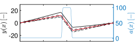
(a) with scaling

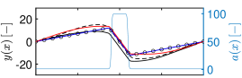
(b) without scaling

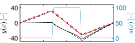
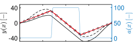
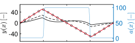
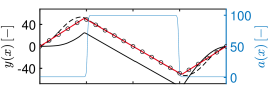
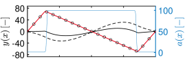
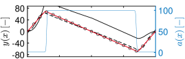
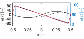
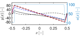
Figure 5: The ANN predictions for the solution field at the end of 30000 epochs and comparison to ABAQUS results (discrete circular markers). The light blue line represents the smoothed material property distribution. The left column belongs to the results with scaling and the right column without scaling. Dashed curves have a learning rate of 0.001 and continuous ones 0.01 for the adam optimizer. Black curves give results for no Fourier feature, whereas dark blue and red for low- and high-frequency Fourier features with a single and the first 10 integer multiples of the reciprocal base vector, respectively.

The training histories of the normalized loss function are given in Fig. 7. The loss for the approximate periodic boundary condition treatment does not provide an accurate prediction, no matter the learning rate. Thus, without Fourier features, the solution struggles to converge. For the loss computations with the Fourier features, for which there is an exact imposition of the periodic boundary conditions, large fluctuations are observed in the stochastic gradient descent phase. On the other hand, in the L-BFGS optimization phase, the loss reduces monotonically. Figure 8 demonstrates that although a lower learning rate generally shows better performance in terms of convergence, with a higher learning rate, convergence is reached at a higher speed.

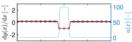
(a) with scaling

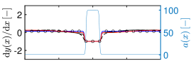
(b) without scaling

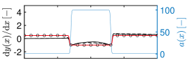
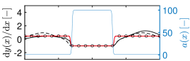
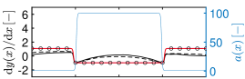
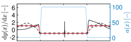
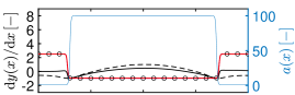
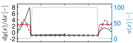
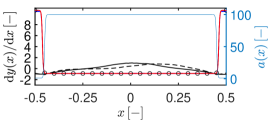
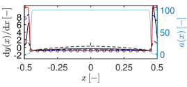
Figure 6: The ANN predictions for the solution field derivative at the end of 30000 epochs and comparison to ABAQUS results (discrete circular markers). The light blue line represents the smoothed material property distribution. The left column belongs to the results with scaling, and the right column is without scaling. Dashed curves have a learning rate of 0.001 and continuous ones 0.01 for the adam optimizer. Black curves give results for no Fourier feature, whereas dark blue and red for low- and high-frequency Fourier features with a single and the first 10 integer multiples of the reciprocal base vector, respectively.

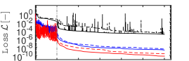
(a) with scaling

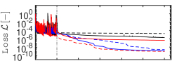
(b) without scaling

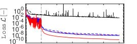
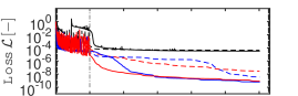
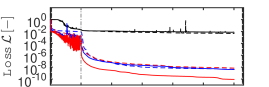
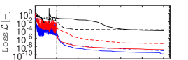
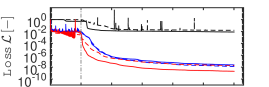
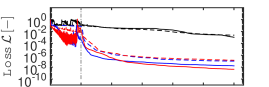
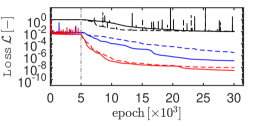
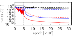
Figure 7: Training history of the loss function for the cell-problem PINN solution. The first 5000 epochs (marked with a vertical red dashed line) belong to adam optimizer, whereas the rest to L-BFGS. The left column belongs to the results with scaling and the right without scaling. Dashed results have a learning rate of 0.001 and continuous lines of 0.01. Black curves give results for no Fourier feature, whereas dark blue and red for low- and high-frequency Fourier features with a single and the first 10 integer multiples of the reciprocal base vector, respectively.

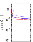
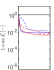
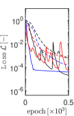
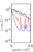
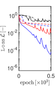
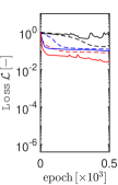
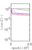
Figure 8: Training history of the loss function for the cell-problem PINN solution for the first 500 adam epochs. In the results, the top row belongs to the results with scaling and the bottom without scaling. Dashed results have a learning rate of 0.001 and continuous lines of 0.01. Black curves give results for no Fourier feature, whereas dark blue and red for low- and high-frequency Fourier features with a single and the first 10 integer multiples of the reciprocal base vector, respectively.

The effective property predictions at the end of 30000 epochs as a function of inclusion volume fraction is given in Fig. 9. In accordance with the solution field distributions and the loss diagrams, neural networks with a Fourier feature layer provide accurate predictions showing excellent agreement with the finite element solutions. The integrated, effective properties can be equivalently computed using Eq. (22). As anticipated, the computed effective properties are closer to the Reuss (harmonic) average. The reason for the discrepancy is the diffuse interface condition considered in the finite element and neural network solutions.

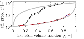
(a) with scaling

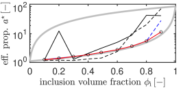
(b) without scaling

Figure 9: ANN solution of the effective properties $a^{\star}$ at the end of 30000 epochs and its comparison with Voigt (arithmetic average) and Reuss (geometric average) analytical bounds, and ABAQUS solution given in circle markers, which is in agreement with the integral given in Eq. (22). The left column belongs to the results with scaling and the right without scaling. Dashed results have a learning rate of 0.001 and continuous lines of 0.01. Black curves give results for no Fourier feature, whereas dark blue and red for low- and high-frequency Fourier features with a single and the first 10 integer multiples of the reciprocal base vector, respectively.

3.3 Two-dimensional Problems

We now consider the problem of finding the solution to Eq. (5) in a 2D system. At the microscale, we assume isotropy for each constituent such that $a_{im}(\boldsymbol{x})=a(\boldsymbol{x})\,\delta_{im}$. In effect, the source term $\partial a_{im}(\boldsymbol{x})/\partial x_{i}$ satisfies the relation $\partial a_{im}(\boldsymbol{x})/\partial x_{i}=\partial a(\boldsymbol{x})/\partial x_{m}$. Finding the solution $\chi^{m}(\boldsymbol{x})$ for the source term for $m$ allows computation of the $m^{\mathrm{th}}$ column vector of the effective property tensor $\boldsymbol{a}^{\star}$, see Eq. (4).

For 2D, the two load cases required are those with two source terms defined in terms of property field gradients $f^{1}=\partial a(\boldsymbol{x})/\partial x_{1}$ and $f^{2}=\partial a(\boldsymbol{x})/\partial x_{2}$. Thus, in view of Eq. (4) with the chosen Cartesian basis, the computation of the components $a^{\star}_{11}$ and $a^{\star}_{21}$ requires the solution $\chi^{1}(\boldsymbol{x})$ for the source term $f^{1}$ which gives

$$a^{\star}_{11}=\dfrac{1}{|\mathcal{V}|}\,\int_{\mathcal{V}}a_{11}\left[1+\dfrac{\partial\chi^{1}(\boldsymbol{x})}{\partial x_{1}}\right]\mathrm{d}V\text{ and }a^{\star}_{21}=\dfrac{1}{|\mathcal{V}|}\,\int_{\mathcal{V}}a_{22}\,\dfrac{\partial\chi^{1}(\boldsymbol{x})}{\partial x_{2}}\mathrm{d}V\,.$$ (24)

The solution $\chi^{2}(\boldsymbol{x})$ obtained for the source term $f^{2}$, on the other hand, allows computation of $a^{\star}_{22}$ and $a^{\star}_{12}=a^{\star}_{21}$, respectively, with

$$a^{\star}_{22}=\dfrac{1}{|\mathcal{V}|}\,\int_{\mathcal{V}}a_{22}\left[1+\dfrac{\partial\chi^{2}(\boldsymbol{x})}{\partial x_{2}}\right]\mathrm{d}V\text{ and }\quad a^{\star}_{12}=\dfrac{1}{|\mathcal{V}|}\,\int_{\mathcal{V}}a_{11}\,\dfrac{\partial\chi^{2}(\boldsymbol{x})}{\partial x_{1}}\mathrm{d}V\,.$$ (25)

The matrix $a_{\mathrm{m}}$ and inclusion $a_{\mathrm{i}}$ properties are selected as $a_{\mathrm{m}}=1$ and $a_{\mathrm{i}}=2$, respectively. We consider the following regularized property distribution

$$a(\boldsymbol{x})=a_{\mathrm{m}}+\dfrac{a_{\mathrm{i}}-a_{\mathrm{m}}}{2}\left[1-\tanh\left(\dfrac{|\boldsymbol{x}-\boldsymbol{x}_{\mathrm{i}}|-r}{\xi}\right)\right]\,.$$ (26)

Here, $\boldsymbol{x}_{\mathrm{i}}$ denotes the position of the inclusion and $r$ its radius. As before, $\xi$ is the regularization parameter that controls the sharpness of the phase interface.

In the following, through the solution of the cell problems with the source terms $f^{1}$ and $f^{2}$ for the $\mathcal{V}-$periodic corrector functions $\chi^{1}(\boldsymbol{x})$ and $\chi^{2}(\boldsymbol{x})$, respectively, we compute $\boldsymbol{a}^{\star}$ for the selected microstructures. The gradients of $\chi^{1}(\boldsymbol{x})$ and $\chi^{2}(\boldsymbol{x})$, required in Eqs. (24) and (25), are obtained from the differentiable ANN solution.

3.3.1 Two-dimensional Square Lattice

We start by considering a single primitive unit cell with a single central circular inclusion. Inclusion volume fractions of $\phi_{\mathrm{i}}=\{0.1,0.2,0.3,0.4,0.5,0.6\}$ are considered. In view of Table 1 and Fig. 1 we consider $L=\rvert\boldsymbol{c}_{1}\rvert=\rvert\boldsymbol{c}_{2}\rvert=200\xi$ with the regularization parameter $\xi=1$.

With Neumann’s principle and the second-order tensor formalism for the property tensor, such microstructures possess isotropic macroscopic properties [47, 48] leading to $\boldsymbol{a}^{\star}=a^{\star}_{11}\,\boldsymbol{1}$ with $a^{\star}_{11}=a^{\star}_{22}$ and $a^{\star}_{12}=a^{\star}_{21}=0$. Thus, it suffices to find the solution to one of the source terms only. Here, we use $f^{1}=\partial a(\boldsymbol{x})/\partial x_{1}$. Individually scaled partial differential equations are considered in the loss term. PBCs are exactly satisfied through low- and high-frequency Fourier features with a single and the first 10 integer multiples of the reciprocal base vector. 25600 collocation points are used. For the adam optimizer, a learning rate of 0.010 is used.

Fig. 10 depicts the contour plots for the property field $a(\boldsymbol{x})$, the source term $\partial a(\boldsymbol{x})/\partial x_{1}$, and the ANN solution fields $\chi(\boldsymbol{x})$ and $|\boldsymbol{\nabla}\chi|$ at the end of 30000 epochs for high-frequency Fourier features. The results are compared to high-resolution finite element simulations conducted with ABAQUS; see Fig. 11. The finite element model includes 260000 linear quadrilateral elements and 260401 nodes. A local element refinement is applied at the diffuse interface zone. As in the case of 1D, the finite element solutions are assumed to correspond to the ground truth. It is observed that high-frequency Fourier features with the first 10 integer multiples of the reciprocal base vector lead to a better agreement with the ground truth. The training histories for the normalized loss function given in Fig. 12 support this observation.

Fig. 13 shows the ANN predictions for the effective property $a^{\star}_{11}$ and its comparison to the ABAQUS solution as well as the analytical truncated series expansion solution of Godin [49] cited in [50]; see C.1. The ANN predictions agree excellently with the finite element simulation results for both low- and high-frequency Fourier feature solutions. The discrepancy between the analytical solutions is, as before, the sharp interface assumption considered in the latter.

Figure 10: The contour plots for the input, the property field $a(\boldsymbol{x})$ with $\boldsymbol{a}(\boldsymbol{x})=a(\boldsymbol{x})\,\boldsymbol{1}$ and $\xi=1$ (row 1) and the source term $\partial a(\boldsymbol{x})/\partial x_{1}$ (row 2), and the PINN solution, $\chi(\boldsymbol{x})$ (row 3) and $|\boldsymbol{\nabla}\chi|$ (row 4), fields of the cell-problem for periodic unit cell $\mathcal{S}_{1}$. Here high-frequency Fourier features with the first 10 integer multiples of the reciprocal base vector are considered. The unit cell constitutes a matrix with inclusions in the form of circular disks positioned at Bravais lattice points with corresponding inclusion volume fractions $\phi_{\mathrm{i}}=\{0.1,0.2,0.3,0.4,0.5,0.6\}$ demonstrated in ascending order from left to right. The intervals [min, max] of the contour plots are: for the first row $[0,100]$, for the second row $[-49.5,49.5]$, for the third row, from left to right, $[0,73]$, $[0,101]$, $[0,122]$, $[0,140]$, $[0,154]$ and (d) $[0,164]$, for the fourth row, from left to right, $[0,1.1]$, $[0,1.5]$, $[0,2.1]$, $[0,3.0]$, $[0,4.5]$ and (d) $[0,8.1]$.

Figure 11: The contour plots for the absolute error in the ANN prediction for $\chi(\boldsymbol{x})$ in comparison to the finite element solution. The top and the bottom rows give low- and high-frequency Fourier features with a single and the first 10 integer multiples of the reciprocal base vector, respectively.

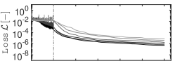
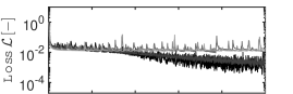
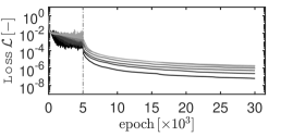
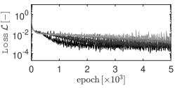
Figure 12: Training history of the normalized loss function for the ANN solutions. The first 5000 epochs (marked with a vertical dashed line) belong to adam optimizer, whereas the rest to L-BFGS. From dark to light colors, the volume fraction changes from 0.10 to 0.60. The top and the bottom rows give low- and high-frequency Fourier features with a single and the first 10 integer multiples of the reciprocal base vector, respectively.

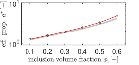
(a) low-frequency

(b) high-frequency

Figure 13: ANN prediction for the effective properties $a^{\star}$ and comparison with ABAQUS solution as well as the truncated series expansion solution of Godin [49] given in [50] for sharp interface conditions; see C.1. The left and the right rows give low- and high-frequency Fourier features with a single and the first 10 integer multiples of the reciprocal base vector, respectively.

We continue our studies on the 2D square lattice with periodic and stochastic disk distributions resulting in an inclusion fraction slightly above $\phi_{i}=0.30$. The phase distribution and the source terms are depicted in see Fig. 14. Since a random structure with a relatively small volume element is considered, an anisotropic property is anticipated. Thus, solutions to both source terms are considered, yielding the complete property tensor components. 65536 collocation points with 50$\times$3 and 100$\times$6 ANN architectures are used in training. In both cases, high-frequency Fourier features with the first 10 integer multiples of the reciprocal base vector are considered.

Considering the stochastic nature of the ANN training process and the absence of ground truth, we reverted to repeated solutions. For each architecture, the ANN is trained three times. The computed effective property tensor components with a chosen basis that conforms to square dimensions are given in Table B11 in Appendix B. As also demonstrated by the training scaled loss history plots given in Fig. 16, 100$\times$6 ANN architecture gives results with higher accuracy in precision with the following representations in terms of mean and standard deviation in four decimal points for each component with $a_{11}=2.2969\pm 0.0018$, $a_{12}=-0.0261\pm 0.0002$, $a_{21}=-0.0296\pm 0.0010$, $a_{22}=2.4012\pm 0.0022$. Corresponding solution fields for the applied source terms are given in Fig. 15. In light of our computations, the following representation in two decimal points constitutes an accurate representation of the symmetric effective property tensor in matrix form, revealing a small anisotropy.

$$\left[\boldsymbol{a}^{\star}\right]=\left[\begin{array}[]{rr}2.30&-0.03\\ -0.03&2.40\\ \end{array}\right]\,.$$ (27)

(a) $a(\boldsymbol{x})$

(b) $f^{1}=\partial a(\boldsymbol{x})/\partial x_{1}$

(c) $f^{2}=\partial a(\boldsymbol{x})/\partial x_{2}$

min  

Figure 14: The contour plots for the property (a) and source terms as property derivatives along $x-$ and $y-$directions for the square periodic unit cell with random disk distribution. The intervals [min, max] of the contour plots are (a) $[1,100]$, (b) and (c) $[-49.5,49.5]$.

(a) $\chi(\boldsymbol{x})$ for $f^{1}$

(b) $|\boldsymbol{\nabla}\chi(\boldsymbol{x})|$ for $f^{1}$

(c) $\chi(\boldsymbol{x})$ for $f^{2}$

(d) $|\boldsymbol{\nabla}\chi(\boldsymbol{x})|$ for $f^{2}$

min  

Figure 15: The contour plots for the ANN solution $\chi(\boldsymbol{x})$ for (a) and (c) and the flux norm $|\boldsymbol{\nabla}\chi(\boldsymbol{x})|$ for (b) and (d) fields of the cell-problem for the square periodic unit cell. The intervals [min, max] of the contour plots are (a) $[0,55]$, (b) $[0,3.6]$ (c) $[0,55]$, and (d) $[0,5.3]$. Results are obtained using a 100$\times$6 architecture with high-frequency Fourier features with the first 10 integer multiples of the reciprocal base vector.

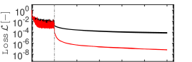
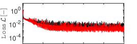
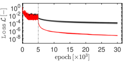
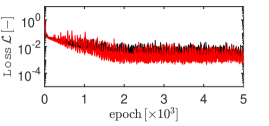
Figure 16: Training history of the normalized loss function for the ANN solutions with 50$\times$3 (black) and 100$\times$6 (red) architectures for the source terms $f^{1}$ and $f^{2}$ for three random trials each. The first 5000 epochs (marked with a vertical dashed line) belong to adam optimizer, whereas the rest to L-BFGS. High-frequency Fourier features with the first 10 integer multiples of the reciprocal base vector are used.

3.3.2 Two-dimensional Centered Rectangular Lattice

In this part, our applications focus on the centered rectangular lattice with $L_{1}/L_{2}=3$ where $L_{1}=\rvert\boldsymbol{c}_{1}$ and $L_{2}=\rvert\boldsymbol{c}_{2}$. We consider the inclusion volume fraction of $\phi_{\mathrm{i}}=\{0.3\}$. The area of the primitive unit cell is arranged to be equal to the square unit cell considered in the previous example with $L_{1}\,L_{2}=L^{2}$. This provides identical radii of the circular inclusion for both cases for the same inclusion volume fraction. We investigate hexagonal, rhombic, and rectangular unit cells, which are referred to as $\mathcal{R}^{\mathrm{c}}_{1}$, $\mathcal{R}^{\mathrm{c}}_{2}$ and $\mathcal{R}^{\mathrm{c}}_{3}$, respectively; see Fig.  1. The direct and the reciprocal unit cell vectors given for $\mathcal{R}^{\mathrm{c}}_{1}$ and $\mathcal{R}^{\mathrm{c}}_{2}$ are not orthogonal; see Table 1. For the rectangular unit cell $\mathcal{R}^{\mathrm{c}}_{3}$, however, they are; with $\boldsymbol{a}_{i}=\boldsymbol{c}_{i}$ and $\boldsymbol{b}_{i}=2\pi\boldsymbol{c}_{i}/|\boldsymbol{c}_{i}|^{2}$ for $i=1,2$. In the ANN training, 65536 collocation points are used for $\mathcal{R}^{\mathrm{c}}_{1}$ and $\mathcal{R}^{\mathrm{c}}_{2}$ whereas for $\mathcal{R}^{\mathrm{c}}_{3}$ which has double the area, the number of collocation points are doubled. Learning rates of 0.001 and 0.010 with 50$\times$3 and 100$\times$6 ANN architectures. Like before, considering the stochastic nature of the ANN training process and the absence of ground truth, we reverted to repeated solutions. For each architecture, the ANN is trained three times. For $\mathcal{R}^{\mathrm{c}}_{1}$ and $\mathcal{R}^{\mathrm{c}}_{2}$, higher accuracy was recorded with a learning rate of 0.001 with 100$\times$6 ANN architecture possessing low-frequency Fourier features. For $\mathcal{R}^{\mathrm{c}}_{3}$, on the other hand, a learning rate of 0.010 with 50$\times$3 ANN architecture possessing high-frequency Fourier features with the first 10 integer multiples of the reciprocal base vector performed best once the consequential training loss is concerned, see Fig.  18.

Fig. 10 depicts the contour plots for the property field $a(\boldsymbol{x})$, the source terms $\partial a(\boldsymbol{x})/\partial x_{1}$ and $\partial a(\boldsymbol{x})/\partial x_{2}$, and the corresponding ANN solution fields $\chi(\boldsymbol{x})$ and $|\boldsymbol{\nabla}\chi|$ at the end of 30000 epochs for the best-performing hyperparameter set for each case. The utilization of Fourier features in conjunction with reciprocal unit cells allows for the satisfaction of periodicity in non-rectangular problem domains. As observed from the contour plots, the choice of the selected unit cell does not change the solution.

The computed effective property tensor components are given in Table B22 in Appendix B for $\mathcal{R}^{\mathrm{c}}_{1}$, $\mathcal{R}^{\mathrm{c}}_{2}$ and $\mathcal{R}^{\mathrm{c}}_{3}$. As demonstrated in Fig. 16, the training losses for all of the unit cells are sufficiently small at the end of 30000 epochs. Nevertheless, learning trends differ due to the difference in the selected ANN hyperparameters. An orthotropic effective property matrix, when using a chosen basis that conforms to rectangular dimensions, is expected, with non-zero diagonal terms and zero off-diagonal terms, resulting in $a^{\star}_{11}\neq a^{\star}_{22}$ and $a^{\star}_{12}=a^{\star}_{21}=0$. For $\mathcal{R}^{\mathrm{c}}_{1}$, a conversion of the tabulated values to mean and standard deviation in four decimal points for each component results in $a_{11}=1.7402\pm 0.0042$, $a_{12}=0.0018\pm 0.0021$, $a_{21}=0.0042\pm 0.0016$, $a_{22}=2.2820\pm 0.0023$. For $\mathcal{R}^{\mathrm{c}}_{2}$, a conversion of the tabulated values to mean and standard deviation for each component results in $a_{11}=1.7423\pm 0.0025$, $a_{12}=-0.0004\pm 0.0012$, $a_{21}=0.0010\pm 0.0013$, $a_{22}=2.2846\pm 0.0026$. Finally, for $\mathcal{R}^{\mathrm{c}}_{3}$, this gives $a_{11}=1.7378\pm 0.0008$, $a_{12}=0.0000\pm 0.0000$, $a_{21}=0.0004\pm 0.0014$, $a_{22}=2.2946\pm 0.0023$. These results show a good agreement between the solutions devising different unit cells. In light of our computations, the following representation in two decimal points emerges as a good approximation for the symmetric effective property tensor in matrix form, revealing anisotropy,

$$\left[\boldsymbol{a}^{\star}\right]=\left[\begin{array}[]{ccc}1.74&0.00\\ 0.00&2.29\\ \end{array}\right]\,.$$ (28)

min  

Figure 17: The contour plots for the input, the property field $a(\boldsymbol{x})$ with $\boldsymbol{a}(\boldsymbol{x})=a(\boldsymbol{x})\,\boldsymbol{1}$ and $\xi=1$ (row 1) and the source term $\partial a(\boldsymbol{x})/\partial x_{1}$ (row 2), and the corresponding ANN solution, $\chi(\boldsymbol{x})$ (row 3) and $|\boldsymbol{\nabla}\chi|$ (row 4), and the source term $\partial a(\boldsymbol{x})/\partial x_{2}$ (row 5), and the corresponding ANN solution, $\chi(\boldsymbol{x})$ (row 6) and $|\boldsymbol{\nabla}\chi|$ (row 7) fields of the cell-problem for periodic unit cells $\mathcal{R}^{\mathrm{c}}_{1}$, $\mathcal{R}^{\mathrm{c}}_{2}$ and $\mathcal{R}^{\mathrm{c}}_{3}$ for the best-performing hyperparameter set for each case. The intervals [min, max] of the contour plots are: for the first row $[0,100]$, for the second and fifth rows $[-49.5,49.5]$, for the third row $[0,123]$, for the fourth row $[0,1.5]$, for the sixth row $[0,125]$, for the seventh row $[0,3.7]$.

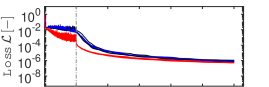
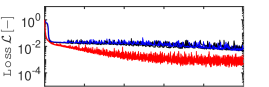
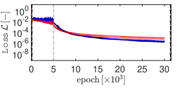
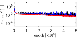
Figure 18: Training history of the normalized loss function for the ANN solution considering unit cells of the cell-problem for periodic unit cells $\mathcal{R}^{\mathrm{c}}_{1}$ (black), $\mathcal{R}^{\mathrm{c}}_{2}$ (blue) and $\mathcal{R}^{\mathrm{c}}_{3}$ (red). For each hyperparameter set, three training sessions are run. The first 5000 epochs (marked with a vertical dashed line) belong to adam optimizer, whereas the rest to L-BFGS. For $\mathcal{R}^{\mathrm{c}}_{1}$ and $\mathcal{R}^{\mathrm{c}}_{2}$, a learning rate of 0.001 with 100$\times$6 ANN architecture possessing low-frequency Fourier features is used, whereas, for $\mathcal{R}^{\mathrm{c}}_{3}$, a learning rate of 0.010 with 50$\times$3 ANN architecture possessing high-frequency Fourier features with the first 10 integer multiples of the reciprocal base vector.

3.3.3 Three-dimensional Simple Cubic Lattice

Finally, we present an application in 3D for a simple cubic lattice with $L=\rvert\boldsymbol{c}_{1}\rvert=\rvert\boldsymbol{c}_{2}\rvert=\rvert\boldsymbol{c}_{3}\rvert=200\xi$ where $\xi=1$ considering two unit cells $\mathcal{C}_{1}$ and $\mathcal{C}_{2}$; see Fig. 1.

The ANN training batch size corresponds to 512000. A learning rate of 0.010 is used with 50$\times$3 ANN architectures with both low- and high-frequency Fourier features, where the ANN is trained three times for each hyperparameter combination.

For the symmetry group possessed by this material microstructure, a spherical second-order effective property tensor is anticipated. Using a chosen basis that conforms to cubic dimensions, this gives non-zero and equal diagonal terms and zero off-diagonal terms, resulting in $a^{\star}_{11}=a^{\star}_{22}=a^{\star}_{33}$ and $a^{\star}_{ij}=0$ for $i\neq j$ and $i,j=1,2,3$. Thus, in our computations, we consider only $x-$gradients of the property field in the source term. The results show that ANNs with high-frequency Fourier features incorporating the first 10 integer multiples of the reciprocal base vector performed best; see Fig.  20. The contour plots for the PINN solution $\chi(\boldsymbol{x})$ the flux norm $|\boldsymbol{\nabla}\chi(\boldsymbol{x})|$ fields of the cell-problem for periodic unit cells $\mathcal{C}_{1}$ and $\mathcal{C}_{2}$ are given for this hyperparameter set are given in Fig. 19. As observed from the contour plots, the choice of the selected unit cell does not change the solution.

The computed effective property tensor components are given in Table B33 in Appendix B for $\mathcal{C}_{1}$ and $\mathcal{C}_{2}$. For the more accurate solution with high-frequency Fourier features, incorporating the first 10 integer multiples of the reciprocal base the mean and standard deviation for the tabulated effective property matrix components result in $a_{11}=2.4550\pm 0.0016$, $a_{12}=0.0001\pm 0.0001$, $a_{13}=-0.0001\pm 0.0002$, for $\mathcal{C}_{1}$, and in $a_{11}=2.4553\pm 0.0020$, $a_{12}=0.0001\pm 0.0000$, $a_{13}=0.0000\pm 0.0002$, for $\mathcal{C}_{2}$. These results show a good agreement between the solutions devising different unit cells. Considering 0.30 inclusion fraction but a sharp interface condition, the truncated series expansion solution of Lam [51] cited in [50], given in C.2 gives $a^{\star}=2.2742$. Similar to our observations for 1D and 2D square lattices with regular circular inclusion distribution for which analytical solutions exist, the ANN solution for the main diagonal term $a^{\star}_{11}$ results in a slightly larger prediction. This discrepancy is due to the utilized diffuse interface assumption. The following representation in matrix form in two decimal points emerges as a good approximation for the effective property tensor

$$\left[\boldsymbol{a}^{\mathcal{C}}\right]=\left[\begin{array}[]{ccc}2.46&0.00&0.00\\ 0.00&2.46&0.00\\ 0.00&0.00&2.46\\ \end{array}\right]\,.$$ (29)

(a) $a(\boldsymbol{x})$

(b) $f^{1}=\partial a(\boldsymbol{x})/\partial x_{1}$

(c) $\chi^{1}(\boldsymbol{x})$ for $f^{1}$

(d) $|\boldsymbol{\nabla}\chi^{1}(\boldsymbol{x}|$ for $f^{1}$

min  

Figure 19: The contour plots for the input, the property field $a(\boldsymbol{x})$ with $\boldsymbol{a}(\boldsymbol{x})=a(\boldsymbol{x})\,\boldsymbol{1}$ and $\xi=1$ (row 1) and the source term $\partial a(\boldsymbol{x})/\partial x_{1}$, and the corresponding ANN solution for high-frequency Fourier features with the first 10 integer multiples of the reciprocal base vector. The intervals [min, max] of the contour plots are (a) $[1,100]$, (b) $[-49.5,49.5]$ (c) $[0,158]$ and (d) $[0,5.8]$.

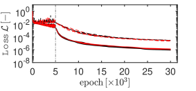
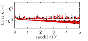
Figure 20: Training history of the normalized loss function for the 3D simulations with unit cells $\mathcal{C}_{1}$ (black) and $\mathcal{C}_{2}$ (red). Continuous lines belong to the ANN solution for high-frequency Fourier features, whereas dashed ones are low-frequency. For each hyperparameter set, three training sessions are conducted. TThe First 5000 epochs (marked with a vertical dashed line) belong to adam optimizer, whereas the rest 25000 to L-BFGS.

4 Conclusion

We applied physics-informed neural networks (PINNs) to determine effective (macroscopic) properties of heterogeneous media using first-order two-scale periodic asymptotic homogenization. A relatively large phase contrast is aimed at. A generic divergence-type elliptic equation is considered to this end which applies to a broad range of physics problems, including electrostatics, magnetostatics, steady-state (time-independent) heat and electrical conduction, and anti-plane elasticity. The unit cell problem for the elliptic equation can be solved up to a constant. The reliance on the standard integral solution for the property tensors on only the gradient of the solution field dismissed the requirement for uniqueness in the solution. This, together with the absence of Dirichlet boundary conditions, resulted in a lossless boundary condition application. ANN architectures with an input-transfer layer (Fourier feature mapping) materializing reciprocal lattice vectors are considered. This allowed an exact imposition of periodic boundary conditions for periodic domains with arbitrary and nonrectangular shapes pertaining to crystalline arrangements defined with different Bravais lattices and improved convergence of high-frequency functions during training once integer multiples of the reciprocal basis in the Fourier mapping are considered. As illustrative examples, we considered applications in one, two, and three dimensions with various regular and stochastic composites. We summarized the influence of the utilized ANN architecture and hyperparameters on the prediction quality.

Appendix A Implementing Periodic Boundary Conditions in Test Cases

In this section, we provide further evaluations of the effectiveness of Fourier features in incorporating periodic boundary conditions. Some of these problems are discussed in Ref. [30]. In all the problems training is performed using 5000 adam optimization steps, followed by 25000 L-BFGS optimization steps.

A.1 Approximation of a One-dimensional Periodic Function

The first selected problem is the ANN approximation of a 1D periodic function. To this end, we select the following function [30]

$$u(x)=\sin(2\pi x+0.25\pi)+\cos(9\pi x+0.10\pi)-2\sin(7\pi x+0.33\pi)\,,$$ (30)

which is periodic over the domain $\Omega=\{x:0\leq x\leq 2\}$.

In the solution to this problem, ANN density and depth are taken as 50 and 3, respectively. 512 points are sampled from the domain. The learning rate is taken as 0.001 and 0.010.

Figs. 21 and 22 demonstrates that ANN with high-frequency Fourier features using the first 10 integer multiples of the reciprocal base vector performs the best in approximating the function in both the convergence rate and the final accuracy. The training loss at the end of 30000 epochs is nearly four orders of magnitude larger for ANNs without Fourier features.

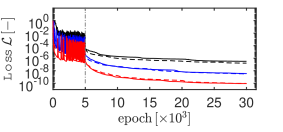
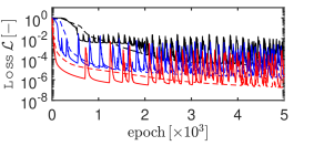
Figure 21: Training history of the normalized loss function for ANN approximation of the 1D periodic function given in Eq. (30), see Fig. 22. The First 5000 epochs (marked with a vertical dashed line) belong to adam optimizer, whereas the rest to L-BFGS. In the numerical trials learning rates of 0.001 (dashed lines) and 0.010 (continuous lines) are used. Black curves give results for no Fourier feature, whereas dark blue and red for low- and high-frequency Fourier features with a single and the first 10 integer multiples of the reciprocal base vector, respectively.

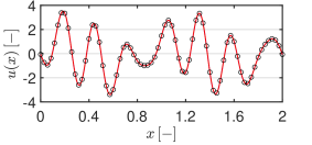
(a) DNN approximation to Eq. (30)

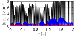
(b) absolute error in DNN soln.

Figure 22: Plots for the 1D periodic function given in Eq. (30) and its ANN approximation (left) and absolute error in the ANN approximation (right) over the problem domain $x\in[0,2]$. Results for a learning rate of 0.010 are demonstrated. Black curves give results for no Fourier feature, whereas dark blue and red for low- and high-frequency Fourier features with a single and the first 10 integer multiples of the reciprocal base vector, respectively.

A.2 Two-dimensional Helmholz Problem with Periodic Boundary Conditions

In this problem, we solve the following Helmholz equation

$$\dfrac{\partial^{2}u}{\partial x^{2}}+\dfrac{\partial^{2}u}{\partial y^{2}}-\lambda u=f(x,y)\,,$$ (31)

which is $x-$ and $y-$periodic over the square domain $\Omega=\{(x,y):0\leq x\leq 4,0\leq y\leq 4\}$. The parameter $\lambda$ is selected as $\lambda=10$. Following Ref. [30], the source term $f(x,y)$ is selected to give the solution $u(x,y)$ of Eq. (31) as

$$u(x,y)=-[1.5\cos(\pi x+0.0.4\pi)+2\cos(2\pi x-0.2\pi)][1.5\cos(\pi y+0.0.4\pi)+2\cos(2\pi y-0.2\pi)]\,.$$ (32)

In the solution to this problem, the ANN density and depth are taken as 50 and 3, respectively. 25600 points are sampled from the domain. The learning rate is taken as 0.010.

The training loss, the solution, and the error involved with respect to the exact solution are given in Figs. 23 and 24, respectively. The results demonstrate that ANN with high-frequency Fourier features using the first 10 integer multiples of the reciprocal base vector performs better in approximating the function in both the convergence rate and the final accuracy.

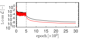
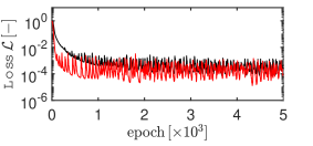
Figure 23: Training history of the normalized loss function for ANN solution for the 2D Helmholz problem given in Eq. (32), see Fig. 24. The First 5000 epochs (marked with a vertical dashed line) belong to adam optimizer, whereas the rest to L-BFGS. ANN with low-(black) and high-frequency (red) Fourier features respectively using a single and the first 10 integer multiples of the reciprocal base vector are considered.

(a) low-frequency

(b) high-frequency

min  

Figure 24: Contours for the ANN solution (left) and its absolute error with respect to the exact solution given in Eq. (32) (right) for the 2D Helmholz problem over $[0,4]\times[0,4]$ problem domain. ANN with low-(a) and high-frequency (b) Fourier features using a single and the first 10 integer multiples of the reciprocal base vector are considered. The intervals [min, max] of the contour plots are $[-12,7.5]$ and $[0,2.0\times 10^{-4}]$ for (a) and for $[-12,7.5]$ and $[0,3.7\times 10^{-5}]$ (b) for the solution and the absolute error, respectively.

A.3 Approximation of a Two-dimensional Periodic Function

We develop an ANN approximation of a 2D periodic function on a hexagonal lattice in this problem. To this end, we select the following function

$$u(x,y)=\tanh(\sin(\rho\,x^{\prime})+0.1\,\cos(\rho\,x^{\prime})+0.6\,\cos(\rho\,y^{\prime}))\,,$$ (33)

with the transformed coordinates along hexagonal lattice direct vectors $x^{\prime}(x,y)=2\pi/L\,x+2\pi/\sqrt{3}L\,y$ and $y^{\prime}(x,y)=4\pi/\sqrt{3}L\,y$ which is periodic over the selected hexagonal domain. Here $\rho$ is the frequency. In our solutions, $\rho=1$ and $\rho=10$ are tried. In this problem, $L$ is selected as 200.

In solving this problem, the ANN density and depth are taken as 50 and 3, respectively. 25600 points are sampled from the domain. The learning rate is taken as 0.010.

The solution and error involved with respect to the exact solution and the training losses are given in Figs. 25 and 26. The results show that using low-frequency Fourier features improves the performance of the ANN when $\rho=1$ while using high-frequency Fourier features with the first 10 integer multiples of the reciprocal base vector improves performance for $\rho=10$ in both convergence rate and accuracy.

min  

Figure 25: Contours for the ANN solution (left) and its absolute error (right) for the approximation of the 2D periodic function given in Eq. (33) for $\rho=1$ (top) and $\rho=10$ (bottom). Two primitive unit cells $\mathcal{H}_{1}$ and $\mathcal{H}_{2}$ with a hexagonal Bravais lattice are considered. The intervals [min, max] of the contour plots for the top row: $[-9.2,9.2]$ and $[0,1.8\times 10^{-5}]$, $[-9.2,9.2]$ and $[0,2.1\times 10^{-5}]$, bottom row: $[-9.2,9.2]$ and $[0,1.9\times 10^{-4}]$, $[-9.2,9.2]$ and $[0,1.9\times 10^{-4}]$ for the solution and the absolute error, respectively.

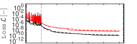
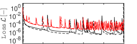
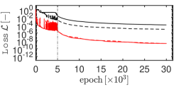
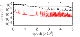
Figure 26: Training history of the normalized loss function for the approximation of the 2D periodic function given in Eq. (33) for $\rho=1$ (top) and $\rho=10$ (bottom) and two primitive unit cells $\mathcal{H}_{1}$ (continuous) and $\mathcal{H}_{2}$ (dashed) considering ANNs with low-(black) and high-frequency (red) Fourier features respectively using a single and the first 10 integer multiples of the reciprocal base vector.

Appendix B Further Results

In this section, additional predictions made using Artificial Neural Networks (ANN) are presented in Tables B11, B22 and B33.

Table B1: ANN predictions with two different architectures for the source term $f^{1}$ and $f^{2}$ for the random and periodic inclusion distribution considering a square lattice. For $f^{1}$ the subscript $i=1$, otherwise $i=2$. Results are obtained using high-frequency Fourier features with the first 10 integer multiples of the reciprocal base vector.

source term	architecture	training ID	$a^{\star}_{1i}$	$a^{\star}_{2i}$
$f^{1}$	50$\times$3	1	2.29216298	0.03443467
		2	2.31131626	0.02962746
		3	2.30685852	0.00065440
	100$\times$6	1	2.29740728	$-0.02406874$
		2	2.29496328	$-0.02575189$
		3	2.29844449	$-0.02840626$
$f^{2}$	50$\times$3	1	$-0.01858249$	2.42691608
		2	$-0.03353900$	2.45424801
		3	0.00227923	2.42688176
	100$\times$6	1	$-0.03044871$	$2.39939146$
		2	$-0.02986018$	$2.40368601$
		3	$-0.02852686$	$2.40053253$

Table B2: ANN predictions for the source term $f^{1}$ and $f^{2}$ considering the three different unit cells and centered rectangular lattice. For $\mathcal{R}^{\mathrm{c}}_{1}$ and $\mathcal{R}^{\mathrm{c}}_{2}$, a learning rate of 0.001 with 100$\times$6 ANN architecture possessing low-frequency Fourier features is used, whereas, for $\mathcal{R}^{\mathrm{c}}_{3}$, a learning rate of 0.010 with 50$\times$3 ANN architecture possessing high-frequency Fourier features with the first 10 integer multiples of the reciprocal base vector. For $f^{1}$ the subscript $i=1$, otherwise $i=2$.

source term	unit cell	training ID	$a^{\star}_{1i}$	$a^{\star}_{2i}$
$f^{1}$	$\mathcal{R}^{\mathrm{c}}_{1}$	1	1.74271078	0.00048956
		2	1.73539798	0.00427126
		3	1.74248766	0.00074224
	$\mathcal{R}^{\mathrm{c}}_{2}$	1	1.74130306	$-0.00138061$
		2	1.74509759	0.00094600
		3	1.74036560	$-0.00070005$
	$\mathcal{R}^{\mathrm{c}}_{3}$	1	1.73772220	$-0.00001145$
		2	1.73706130	$-0.00000122$
		3	1.73864375	$-0.00001003$
$f^{2}$	$\mathcal{R}^{\mathrm{c}}_{1}$	1	0.00604348	2.27994320
		2	0.00377181	2.28445564
		3	0.00283645	2.28166015
	$\mathcal{R}^{\mathrm{c}}_{2}$	1	0.00117976	2.28162650
		2	$-0.00035555$	2.28630918
		3	0.00227585	2.28578361
	$\mathcal{R}^{\mathrm{c}}_{3}$	1	$-0.00120572$	2.29766637
		2	0.00162594	2.29669590
		3	0.00067097	2.28941049

Table B3: ANN predictions for the source term $f^{1}$ for considering the two different unit cells $\mathcal{C}_{1}$ and $\mathcal{C}_{2}$ and simple cubic lattice. A learning rate of 0.010 with 50$\times$3 ANN architecture is utilized with low-frequency and high-frequency Fourier features, respectively possessing a single and first 10 integer multiples of the reciprocal base vector.

unit cell	Fourier features	training ID	$a^{\star}_{11}$	$a^{\star}_{21}$	$a^{\star}_{31}$
$\mathcal{C}_{1}$	low-frequency	1	2.59757603	0.00951802	0.00804197
		2	2.63482571	$-0.00019953$	$-0.00224011$
		3	2.53020037	0.00050227	0.00174256
	high-frequency	1	2.45337680	0.00009547	0.00006592
		2	2.45661833	0.00023308	$-0.00030972$
		3	2.45504276	0.00000776	$-0.00020233$
$\mathcal{C}_{2}$	low-frequency	1	2.55916996	0.00283198	0.00495483
		2	2.65327004	0.00095332	0.00479847
		3	2.59437703	$-0.00665691$	0.00356463
	high-frequency	1	2.45392204	0.00009346	0.00023590
		2	2.45781939	0.00010920	$-0.00023763$
		3	2.45432994	0.00011981	0.00010465

Appendix C Analytical Solutions

C.1 Two-dimensional Square Circular Disk Distributions

Square and periodic arrangement of disks possess isotropic effective properties once the considered property tensors are of second order [48]. Thus, the effective property tensor $\boldsymbol{a}^{\star}$ can be represented by a scalar $a^{\star}$ where $\boldsymbol{a}^{\star}=a^{\star}\,\boldsymbol{1}$. For a matrix with circular inclusions with the square and periodic arrangement and respective properties denoted by $a_{\mathrm{m}}$ and $a_{\mathrm{i}}$, the truncated series expansion solution of Godin [49] cited in [50], gives the analytical expression for $a^{\star}$ as

$$a^{\star}=\left[\dfrac{1+\phi_{\mathrm{i}}\,\lambda(\phi_{\mathrm{i}})}{1-\phi_{\mathrm{i}}\,\lambda(\phi_{\mathrm{i}})}\right]\,a_{\mathrm{m}}$$ (34)

with

$$\lambda(\phi_{i})=c_{0}+c_{4}\phi^{4}_{\mathrm{i}}+c_{8}\phi_{\mathrm{i}}^{8}+c_{12}\phi^{12}_{\mathrm{i}}+O(\phi^{16}_{\mathrm{i}})\,.$$

Here, the coefficients $c_{i}$ are functions of $\alpha=[a_{\mathrm{i}}-a_{\mathrm{m}}][a_{\mathrm{i}}+a_{\mathrm{m}}]$ with

$$c_{0} =\alpha\,,$$

$$c_{4} =0.305827\alpha^{3}\,,$$

$$c_{8} =\alpha^{3}[0.0935304\alpha^{2}+0.0133615]\,,$$

$$c_{12} =\alpha^{3}[0.0286042\alpha^{4}+0.437236\alpha^{2}+0.000184643]\,.$$

C.2 Three-dimensional Cubic Sphere Distributions

Coming to the sphere distributions in 3D, the truncated series expansion solution of Lam [51] cited in [50], gives the analytical expression for $a^{\star}$ as

$$a^{\star}=\left[1+\dfrac{3\phi_{\mathrm{i}}}{\gamma(\phi_{\mathrm{i}})}\right]\,a_{m}$$ (35)

with

$$\gamma(\phi_{\mathrm{i}}) =-\dfrac{1}{R_{1}}-\phi_{\mathrm{i}}+1.3045R_{3}\phi_{\mathrm{i}}^{10/3}+0.0723R_{5}\phi_{\mathrm{i}}^{14/3}$$

$$-0.5289R^{2}_{3}\phi_{\mathrm{i}}^{17/3}+0.1526R_{7}\phi_{\mathrm{i}}^{6}+O(\phi^{7}_{\mathrm{i}})\,,$$

where

$$R_{n}=\dfrac{n[a_{\mathrm{m}}-a_{\mathrm{i}}]}{[n+1]a_{\mathrm{m}}+na_{\mathrm{i}}}\,.$$

References

- Esteva et al. [2021] A. Esteva, K. Chou, S. Yeung, N. Naik, A. Madani, A. Mottaghi, Y. Liu, E. Topol, J. Dean, R. Socher, Deep learning-enabled medical computer vision, npj Digit. Med. 4 (2021). doi:10.1038/s41746-020-00376-2.
- Richens et al. [2020] J. G. Richens, C. M. Lee, S. Johri, Improving the accuracy of medical diagnosis with causal machine learning, Nature Communications 11 (2020). doi:10.1038/s41467-020-17419-7.
- Le Glaz et al. [2021] A. Le Glaz, Y. Haralambous, D.-H. Kim-Dufor, P. Lenca, R. Billot, T. C. Ryan, J. Marsh, J. DeVylder, M. Walter, S. Berrouiguet, C. Lemey, Machine learning and natural language processing in mental health: Systematic review, J Med Internet Res 23 (2021) e15708. doi:10.2196/15708.
- Dixon et al. [2020] M. Dixon, I. Halperin, P. Bilokon, Machine Learning in Finance From Theory to Practice, Springer, 2020.
- Lagaris et al. [1998] I. Lagaris, A. Likas, D. Fotiadis, Artificial neural networks for solving ordinary and partial differential equations, IEEE Transactions on Neural Networks 9 (1998) 987–1000. URL: https://doi.org/10.1109%2F72.712178. doi:10.1109/72.712178.
- Cybenko [1989] G. Cybenko, Approximation by superpositions of a sigmoidal function, Mathematics of Control, Signals and Systems 2 (1989) 303–314.
- Hornik et al. [1989] K. Hornik, M. Stinchcombe, H. White, Multilayer feedforward networks are universal approximators, Neural Networks 2 (1989) 359–366. URL: https://www.sciencedirect.com/science/article/pii/0893608089900208. doi:https://doi.org/10.1016/0893-6080(89)90020-8.
- Hornik et al. [1990] K. Hornik, M. Stinchcombe, H. White, Universal approximation of an unknown mapping and its derivatives using multilayer feedforward networks, Neural Networks 3 (1990) 551–560. URL: https://www.sciencedirect.com/science/article/pii/0893608090900056. doi:https://doi.org/10.1016/0893-6080(90)90005-6.
- Lu et al. [2021] L. Lu, X. Meng, Z. Mao, G. E. Karniadakis, DeepXDE: A deep learning library for solving differential equations, SIAM Review 63 (2021) 208–228. URL: https://doi.org/10.1137%2F19m1274067. doi:10.1137/19m1274067.
- Zhang et al. [2019] D. Zhang, L. Lu, L. Guo, G. E. Karniadakis, Quantifying total uncertainty in physics-informed neural networks for solving forward and inverse stochastic problems, Journal of Computational Physics 397 (2019) 108850. URL: https://www.sciencedirect.com/science/article/pii/S0021999119305340. doi:https://doi.org/10.1016/j.jcp.2019.07.048.
- Pang et al. [2019] G. Pang, L. Lu, G. E. Karniadakis, fPINNs: Fractional physics-informed neural networks, SIAM Journal on Scientific Computing 41 (2019) A2603–A2626. URL: https://doi.org/10.1137%2F18m1229845. doi:10.1137/18m1229845.
- Abadi et al. [2015] M. Abadi, A. Agarwal, P. Barham, E. Brevdo, Z. Chen, C. Citro, G. S. Corrado, A. Davis, J. Dean, M. Devin, S. Ghemawat, I. Goodfellow, A. Harp, G. Irving, M. Isard, Y. Jia, R. Jozefowicz, L. Kaiser, M. Kudlur, J. Levenberg, D. Mané, R. Monga, S. Moore, D. Murray, C. Olah, M. Schuster, J. Shlens, B. Steiner, I. Sutskever, K. Talwar, P. Tucker, V. Vanhoucke, V. Vasudevan, F. Viégas, O. Vinyals, P. Warden, M. Wattenberg, M. Wicke, Y. Yu, X. Zheng, TensorFlow: Large-scale machine learning on heterogeneous systems, 2015. URL: https://www.tensorflow.org/, software available from tensorflow.org.
- Paszke et al. [2019] A. Paszke, S. Gross, F. Massa, A. Lerer, J. Bradbury, G. Chanan, T. Killeen, Z. Lin, N. Gimelshein, L. Antiga, A. Desmaison, A. Kopf, E. Yang, Z. DeVito, M. Raison, A. Tejani, S. Chilamkurthy, B. Steiner, L. Fang, J. Bai, S. Chintala, Pytorch: An imperative style, high-performance deep learning library, in: Advances in Neural Information Processing Systems 32, Curran Associates, Inc., 2019, pp. 8024–8035. URL: http://papers.neurips.cc/paper/9015-pytorch-an-imperative-style-high-performance-deep-learning-library.pdf.
- Raissi et al. [2019] M. Raissi, P. Perdikaris, G. Karniadakis, Physics-informed neural networks: A deep learning framework for solving forward and inverse problems involving nonlinear partial differential equations, Journal of Computational Physics 378 (2019) 686–707. doi:https://doi.org/10.1016/j.jcp.2018.10.045.
- Haghighat et al. [2021] E. Haghighat, M. Raissi, A. Moure, H. Gomez, R. Juanes, A physics-informed deep learning framework for inversion and surrogate modeling in solid mechanics, Computer Methods in Applied Mechanics and Engineering 379 (2021) 113741. URL: https://www.sciencedirect.com/science/article/pii/S0045782521000773. doi:https://doi.org/10.1016/j.cma.2021.113741.
- Cuomo et al. [2022] S. Cuomo, V. S. di Cola, F. Giampaolo, G. Rozza, M. Raissi, F. Piccialli, Scientific machine learning through physics-informed neural networks: Where we are and what’s next, 2022. URL: https://arxiv.org/abs/2201.05624. doi:10.48550/ARXIV.2201.05624.
- Lagaris et al. [2000] I. Lagaris, A. Likas, D. Papageorgiou, Neural-network methods for boundary value problems with irregular boundaries, IEEE Transactions on Neural Networks 11 (2000) 1041–1049. doi:10.1109/72.870037.
- Sirignano and Spiliopoulos [2018] J. Sirignano, K. Spiliopoulos, DGM: A deep learning algorithm for solving partial differential equations, Journal of Computational Physics 375 (2018) 1339–1364. URL: https://www.sciencedirect.com/science/article/pii/S0021999118305527. doi:https://doi.org/10.1016/j.jcp.2018.08.029.
- Chen et al. [2020a] J. Chen, R. Du, K. Wu, A comprehensive study of boundary conditions when solving pdes by dnns, arXiv preprint arXiv:2005.04554 (2020a).
- Chen et al. [2020b] J. Chen, R. Du, K. Wu, A comparison study of deep galerkin method and deep ritz method for elliptic problems with different boundary conditions (2020b). URL: https://arxiv.org/abs/2005.04554. doi:10.48550/ARXIV.2005.04554.
- Bargmann et al. [2018] S. Bargmann, B. Klusemann, J. Markmann, J. E. Schnabel, K. Schneider, C. Soyarslan, J. Wilmers, Generation of 3D representative volume elements for heterogeneous materials: a review, Progress in Materials Science 96 (2018) 322–384. doi:https://doi.org/10.1016/j.pmatsci.2018.02.003.
- Soyarslan et al. [2018] C. Soyarslan, S. Bargmann, M. Pradas, J. Weissmüller, 3D stochastic bicontinuous microstructures: Generation, topology and elasticity, Acta Materialia 149 (2018) 326 – 340. doi:https://doi.org/10.1016/j.actamat.2018.01.005.
- Soyarslan et al. [2019] C. Soyarslan, M. Pradas, S. Bargmann, Effective elastic properties of 3d stochastic bicontinuous composites, Mechanics of Materials 137 (2019) 103098.
- Torquato [2002] S. Torquato, Random Heterogeneous Materials: Microstructure and Macroscopic Properties, Interdisciplinary Applied Mathematics 16, 1 ed., Springer-Verlag New York, 2002.
- Fish [2014] J. Fish, Practical Multiscaling, John Wiley and Sons, Chichester, 2014.
- Ngom and Marin [2020] M. Ngom, O. Marin, Fourier neural networks as function approximators and differential equation solvers, 2020. URL: https://arxiv.org/abs/2005.13100. doi:10.48550/ARXIV.2005.13100.
- Gallant and White [1988] R. A. Gallant, H. White, There exists a neural network that does not make avoidable mistakes, in: IEEE 1988 International Conference on Neural Networks, 1988, pp. 657–664 vol.1. doi:10.1109/ICNN.1988.23903.
- Liu [2013] S. Liu, Fourier neural network for machine learning, in: 2013 International Conference on Machine Learning and Cybernetics, volume 01, 2013, pp. 285–290. doi:10.1109/ICMLC.2013.6890482.
- Zhumekenov et al. [2019] A. Zhumekenov, M. Uteuliyeva, O. Kabdolov, R. Takhanov, Z. Assylbekov, A. J. Castro, Fourier neural networks: A comparative study, 2019. URL: https://arxiv.org/abs/1902.03011. doi:10.48550/ARXIV.1902.03011.
- Dong and Ni [2021] S. Dong, N. Ni, A method for representing periodic functions and enforcing exactly periodic boundary conditions with deep neural networks, Journal of Computational Physics 435 (2021) 110242. URL: https://www.sciencedirect.com/science/article/pii/S0021999121001376. doi:https://doi.org/10.1016/j.jcp.2021.110242.
- Göküzüm et al. [2019] F. S. Göküzüm, L. T. K. Nguyen, M.-A. e. Keip, An artificial neural network based solution scheme for periodic computational homogenization of electrostatic problems, Mathematical and Computational Applications 24 (2019). URL: https://www.mdpi.com/2297-8747/24/2/40. doi:10.3390/mca24020040.
- Lukkassen et al. [1995] D. Lukkassen, L.-E. Persson, P. Wall, Some engineering and mathematical aspects on the homogenization method, Composites Engineering 5 (1995) 519 – 531. doi:https://doi.org/10.1016/0961-9526(95)00025-I.
- Bishara et al. [2022] D. Bishara, Y. Xie, W. K. Liu, S. Li, A state-of-the-art review on machine learning-based multiscale modeling, simulation, homogenization and design of materials, Archives of Computational Methods in Engineering (2022) 1886–1784. doi:https://doi.org/10.1007/s11831-022-09795-8.
- Kittel [1953] C. Kittel, Introduction to Solid State Physics, Wiley, 1953.
- Hofmann [2008] P. Hofmann, Solid state physics : an introduction, Physics textbook, Wiley-VCH, 2008.
- Garboczi [1998] E. Garboczi, Finite element and finite difference programs for computing the linear electric and elastic properties of digital images of random materials, 1998.
- Chatzigeorgiou et al. [2014] G. Chatzigeorgiou, A. Javili, P. Steinmann, Unified magnetomechanical homogenization framework with application to magnetorheological elastomers, Mathematics and Mechanics of Solids 19 (2014) 193–211.
- Javili et al. [2013] A. Javili, G. Chatzigeorgiou, P. Steinmann, Computational homogenization in magneto-mechanics, International Journal of Solids and Structures 50 (2013) 4197–4216.
- Karimi et al. [2019] P. Karimi, X. Zhang, S. Yan, M. Ostoja-Starzewski, J.-M. Jin, Electrostatic and magnetostatic properties of random materials, Phys. Rev. E 99 (2019) 022120. URL: https://link.aps.org/doi/10.1103/PhysRevE.99.022120. doi:10.1103/PhysRevE.99.022120.
- Soyarslan et al. [2023] C. Soyarslan, J. Havinga, L. Abelmann, T. van den Boogaard, Asymptotic homogenization in the determination of effective intrinsic magnetic properties of composites, Results in Physics 44 (2023) 106188. URL: https://www.sciencedirect.com/science/article/pii/S2211379722008099. doi:https://doi.org/10.1016/j.rinp.2022.106188.
- Rumelhart et al. [1986] D. E. Rumelhart, G. E. Hinton, R. J. Williams, Learning representations by back-propagating errors, Nature 323 (1986) 533–536. URL: http://doi.org/10.1038/323533a0. doi:10.1038/323533a0.
- Rahimi and Recht [2007] A. Rahimi, B. Recht, Random features for large-scale kernel machines, NeurIPS (2007).
- Tancik et al. [2020] M. Tancik, P. P. Srinivasan, B. Mildenhall, S. Fridovich-Keil, N. Raghavan, U. Singhal, R. Ramamoorthi, J. T. Barron, R. Ng, Fourier features let networks learn high frequency functions in low dimensional domains, 2020. URL: https://arxiv.org/abs/2006.10739. doi:10.48550/ARXIV.2006.10739.
- Lu et al. [2021] L. Lu, R. Pestourie, W. Yao, Z. Wang, F. Verdugo, S. G. Johnson, Physics-informed neural networks with hard constraints for inverse design, 2021. URL: https://arxiv.org/abs/2102.04626. doi:10.48550/ARXIV.2102.04626.
- Zhang et al. [2019] D. Zhang, L. Guo, G. E. Karniadakis, Learning in modal space: Solving time-dependent stochastic pdes using physics-informed neural networks, 2019. URL: https://arxiv.org/abs/1905.01205. doi:10.48550/ARXIV.1905.01205.
- Henkes et al. [2022] A. Henkes, H. Wessels, R. Mahnken, Physics informed neural networks for continuum micromechanics, Computer Methods in Applied Mechanics and Engineering 393 (2022) 114790. doi:10.1016/j.cma.2022.114790.
- Neumann [1885] F. E. Neumann, Vorlesungen über mathematische Physik: Vorlesungen über die Theorie der Elasticität der festen Körper und des Lichtäthers, B. G. Teubner, Leipzig, 1885.
- Nye [1985] J. F. Nye, Physical Properties of Crystals, Clarendon Press, Oxford, 1985.
- Godin [2013] Y. A. Godin, Effective complex permittivity tensor of a periodic array of cylinders, Journal of Mathematical Physics 54 (2013) 053505. URL: http://doi.org/10.1063/1.4803490. doi:10.1063/1.4803490.
- Ren et al. [2018] X. Ren, R. Corcolle, L. Daniel, Bounds and estimates on eddy current losses in soft magnetic composites, Journal of Applied Physics 123 (2018) 235109. URL: http://doi.org/10.1063/1.5031128. doi:10.1063/1.5031128.
- Lam [1986] J. Lam, Magnetic permeability of a simple cubic lattice of conducting magnetic spheres, Journal of Applied Physics 60 (1986) 4230–4235.