Two-Stage Learning For the Flexible Job Shop Scheduling Problem

Abstract

The Flexible Job-shop Scheduling Problem (FJSP) is an important combinatorial optimization problem that arises in manufacturing and service settings. FJSP is composed of two subproblems, an assignment problem that assigns tasks to machines, and a scheduling problem that determines the starting times of tasks on their chosen machines. Solving FJSP instances of realistic size and composition is an ongoing challenge even under simplified, deterministic assumptions. Motivated by the inevitable randomness and uncertainties in supply chains, manufacturing, and service operations, this paper investigates the potential of using a deep learning framework to generate fast and accurate approximations for FJSP. In particular, this paper proposes a two-stage learning framework 2SL-FJSP that explicitly models the hierarchical nature of FJSP decisions, uses a confidence-aware branching scheme to generate appropriate instances for the scheduling stage from the assignment predictions, and leverages a novel symmetry-breaking formulation to improve learnability. 2SL-FJSP is evaluated on instances from the FJSP benchmark library. Results show that 2SL-FJSP can generate high-quality solutions in milliseconds, outperforming a state-of-the-art reinforcement learning approach recently proposed in the literature, and other heuristics commonly used in practice.

1 Introduction

The Flexible Job-shop Scheduling problem (FJSP) is a generalization of the classical Job-shop Scheduling problem (JSP) that appears in a wide-range of application areas including logistics, manufacturing, transportation, and services. FJSP considers a set of jobs, each consisting of a number of ordered tasks that need to be assigned and scheduled on machines such that the maximum time needed to complete all jobs, known as the makespan, is minimized. The FJSP is hard to solve for real-sized instances, even under simplified, deterministic assumptions; it is NP-hard in the strong sense.

The FJSP is composed of two subproblems, an assignment subproblem that assigns tasks to machines, and a scheduling subproblem that determines the sequence and processing schedule of tasks on their selected machines Brandimarte (1993). For a complex problem like the FJSP, concurrent approaches that solve for the assignment and scheduling subproblems simultaneously often fail to provide effective solutions in reasonable runtimes Chaudhry and Khan (2016). Hierarchical approaches, on the other hand, are more common as they reduce the original problem complexity by decomposing it into subproblems that are solved sequentially. A natural hierarchical scheme for solving the FJSP is based on the observation that, when machine assignments are decided, the FJSP reduces to the classical JSP. For that reason, two-stage hierarchical schemes that separate assignment and scheduling decisions have been widely used in the design of efficient heuristic and exact FJSP algorithms (see for example: Fattahi et al. (2007); Xie et al. (2019); Naderi and Roshanaei (2022), and Xie et al. (2019) for a comprehensive review).

While extensive research has been done to solve FJSP using exact and approximate solution techniques, operational realities surrounding its application domain hinder their effective adoption especially in contexts when solutions must be generated under stringent time constraints, i.e. in real time. For example, uncertainty revealed on day-of-operation is a key practical concern that may require immediate replanning of operations. Such uncertainty could stem from either the continuous variations of processing times, and/or the combinatorial presence, or absence, of machines, or jobs for processing. This work focuses on the former aspect that if not addressed properly, could result in machine idling or job delays that can be very costly. To address this issue, planners typically resort to using rule-based, hierarchical, heuristics that can generate approximate solutions very quickly Jun et al. (2019); Kawai and Fujimoto (2005). However, while efficient, the sub-optimality of their solutions could translate into considerable economical losses that are not desirable in practice.

Motivated by the need for fast and effective approximate solutions, the training of machine-learning models as surrogates for solving hard combinatorial optimization problems has gained traction; see Vesselinova et al. (2020) for a survey on the topic. An important challenge in this line of work is related to ensuring the feasibility of predicted solutions. To address this, several approaches have been proposed in the literature including the use of Langrangian loss functions (see for example Kotary et al. (2022); Fioretto et al. (2020); Chatzos et al. (2020)), and incorporating optimization algorithms into differentiable systems (see for example Vinyals et al. (2015); Khalil et al. (2017); Kool et al. (2018); Park et al. (2022)). Another challenge is related to the solution structure that is present in combinatorial problems. For a problem like FJSP, it is common to have multiple, symmetric, solutions since there can be multiple identical machines that can process the same job Ostrowski et al. (2010). Additionally, it is also common to work with solutions that are approximate and not optimal due to the computationally difficulty associated with solving instances to optimality. The presence of these effects could result in datasets that are harder to learn, and therefore, more structured data generation approaches are needed Kotary et al. (2021a).

To this end, this paper proposes 2SL-FJSP, a machine-learning framework that can be used as an optimization proxy for solving FJSP instances in uncertain environments. 2SL-FJSP exploits the problem structure and proposes a two-stage deep-learning approach that learn to map FJSP instances, sampled from a distribution of processing times, to assignment and scheduling solutions that are close to those generated directly via optimization. The two-stage structure of 2SL-FJSP is complemented by a confidence-aware branching scheme that generates instances for the second-stage learning to account for prediction errors in the first stage. 2SL-FJSP also leverages a novel data generation that exploits a novel symmetry-breaking scheme that may facilitate learning significantly.

Contributions

The contributions of this paper can be summarized as follows. (1) It proposes 2SL-FJSP, a two-stage learning framework for the FJSP that exploits its hierarchical nature in providing fast and effective FJSP approximations. (2) 2SL-FJSP introduces a confidence-aware branching scheme to account for prediction errors in the assignment stage and generate a more comprehensive set of instances for the scheduling stage. (3) 2SL-FJSP includes a novel symmetry-breaking data generation approach that alleviates issues in learnability caused by the presence of co-optimal and approximate solutions typically experienced in scheduling problems. The symmetry-breaking scheme breaks the symmetries for all instances uniformly and can be parallelized contrary to prior work. (4) 2SL-FJSP integrates these innovations with state-of-the-art techniques for capturing constraint violations and restoring feasibility. (5) 2SL-FJSP has been evaluated on standard benchmarks and computational results show that, on the experimental setting considered in the paper, it significantly outperforms state-of-the-art heuristic and reinforcement learning approaches. The results also show the critical role of each component.

2 Related Work

Learning for constrained optimization

Deep learning is increasingly being applied to constrained optimization problems. The typical approaches use neural networks to predict permutations or combinations as sequences of actions by using imitation learning or reinforcement learning Vinyals et al. (2015); Khalil et al. (2017); Kool et al. (2018); Park et al. (2022). Other approaches involve using (unrolled) optimization algorithms as differentiable layers in neural networks Amos and Kolter (2017); Agrawal et al. (2019); Vlastelica et al. (2019); Chen et al. (2020); Donti et al. (2021). Additionally, some works regularize the training of the neural network with penalty methods or Lagrangian duality Fioretto et al. (2020); Kotary et al. (2021a); Chatzos et al. (2020). Refer to Bengio et al. (2021); Kotary et al. (2021b); Lei et al. (2022) for more comprehensive reviews.

Learning for Flexible Job Shop Scheduling

Recently, a number of works use deep reinforcement learning (DRL) for Job Shop Scheduling Problems (JSP) Lin et al. (2019); Park et al. (2019); Zhang et al. (2020); Song et al. (2022); Liu et al. (2022). In Lin et al. (2019), a deep Q learning-based method is used to select the priority dispatch rule of JSP. Zhang et al. (2020) represents the disjunctive graph of JSP using graph neural networks to embed the state information and train the RL agent using proximal policy optimization Schulman et al. (2017). Song et al. (2022) extends the work Zhang et al. (2020) to FJSP using heterogeneous graph representation. However, previous DRL works encounter convergence issues when training on large instances. In particular, as shown in Song et al. (2022), increasing the instance size in the DRL training often degrades the performance of the DRL policy on public benchmarks.

Recently, Kotary et al. (2022) explored another direction to learn the mapping from the processing times to optimal schedules by using Lagrangian duality for the job-shop scheduling problem. 2SL-FJSP builds on this work and proposes a two-stage learning framework to approximate the FJSP. 2SL-FJSP explicitly models the hierarchical nature of the FJSP decisions, uses a confidence-aware neural network for the assignment predictions to generate training instances for the scheduling predictions, and proposes a new symmetry-breaking scheme to generate, in parallel, the training data for the scheduling predictions.

3 Preliminaries

The Flexible Job-shop Scheduling Problem

The Flexible Job-shop Scheduling Problem (FJSP) is defined primarily by a set of jobs $J$ and a set of machines $M$. Each job consists of a set of ordered tasks $T$ that need to be processed in a pre-defined sequence. Each task is allowed to be processed on one machine out of a set of alternative machines. The expected duration of task $t$ of job $j$ on machine $m$ is denoted by $d^{m}_{jt}$ and $N=J\times T$ is the set of all tasks.

Model 1 provides a high-level mathematical description of the FJSP with decision variables $z^{m}_{jt}\in\{1,0\}$ indicating whether task $t$ of job $j$ is assigned to machine $m$ for processing, $s^{m}_{jt}\geq 0$ representing the start time of task $t$ of job $j$ on machine $m$, and $C_{max}\geq 0$ representing the maximum completion time of all jobs, also known as the makespan. The FJSP aims at finding task-to-machine assignments and their corresponding schedules such that the makespan is minimized.

The assignment constraints (1b) ensure that a task is processed on a single machine without splitting. The task-precedence constraints (1c) ensure that all tasks are processed following their given order; for simplicity, a higher-indexed task is a predecessor of a lower-indexed task. The machine-precedence constraints (1d) ensure that no two tasks overlap in time if they are assigned to be processed on the same machine. The disjunctive nature of constraints (1d) makes the FJSP hard to solve even for medium-sized instances. It can be modeled in various ways using e.g., Mixed Integer Programming (MIP) and Constraint Programming (CP), each having its own features and merits (e.g., Chaudhry and Khan (2016); Fattahi et al. (2007)). This paper uses a CP approach that is proven to be effective for solving scheduling problems; the corresponding FJSP CP formulation is presented in Appendix A.

Model 1 FJSP Description

$$\mbox{Minimize}\quad C_{max}\qquad$$ (1a)

subject to:

$$\sum_{m\in M_{jt}}z^{m}_{jt}=1\qquad\forall j\in[J],t\in[T]$$ (1b)

$$s^{m}_{jt-1}\geq s^{m}_{jt}+d^{m}_{jt}z^{m}_{jt}\qquad\forall j\in[J],t\in[T],t>0,m\in M_{jt},$$ (1c)

$$s^{m}_{jt}\geq s^{m}_{j^{\prime}t^{\prime}}+d^{m}_{j^{\prime}t^{\prime}}z^{m}_{j^{\prime}t^{\prime}}\quad\vee\quad s^{m}_{j^{\prime}t^{\prime}}\geq s^{m}_{jt}+d^{m}_{jt}z^{m}_{jt},$$ (1d)

$$\qquad\qquad\forall j,j^{\prime}\in[J],t,t^{\prime}\in[T],j\neq j^{\prime},m\in M_{jt},$$

$$C_{max}\geq s^{m}_{jt}+d^{m}_{jt}z^{m}_{jt}\qquad\forall j\in[J],t\in[T],t=0,m\in M_{jt},$$ (1e)

$$z^{m}_{jt}\in\{0,1\}\qquad\forall j\in[J],t\in[T],m\in M_{jt},$$ (1f)

$$s^{m}_{jt}\geq 0\qquad\forall j\in[J],t\in[T],m\in M_{jt}.$$ (1g)

The Job Shop Scheduling Problem

The Job Shop Scheduling (JSP) is a special case of the FJSP, with each task having a single machine option for processing. This reduces the decision space to finding task schedule given a known assignment. Model 2 presents a high-level description of the JSP with decision variables $s_{jt}$ and $C_{max}$ representing the start time of each task and the makespan, respectively. The description of the task-precedence constraints (2b) and the machine-precedence constraints (2c) is identical to that of FJSP; no machine selection is needed in JSP since a task can be processed only on a specified machine.

Model 2 JSP Description

$$\mbox{Minimize}\quad C_{max}\qquad$$ (2a)

subject to:

$$s_{jt-1}\geq s_{jt}+d_{jt}\qquad\forall j\in[J],t\in[T],t>0,$$ (2b)

$$s_{jt}\geq s_{j^{\prime}t^{\prime}}+d_{j^{\prime}t^{\prime}}\quad\vee\quad s_{j^{\prime}t^{\prime}}\geq s_{jt}+d_{jt}\qquad$$ (2c)

$$\qquad\forall j,j^{\prime}\in[J],t,t^{\prime}\in[T],j\neq j^{\prime},\sigma_{jt}=\sigma_{j^{\prime}t^{\prime}}$$

$$C_{max}\geq s_{jt}+d_{jt}\qquad\forall j\in[J],t\in[T],t=0$$ (2d)

$$s_{jt}\geq 0\qquad\forall j\in[J],t\in[T],m\in M_{jt}.$$ (2e)

4 The Learning Task for the FJSP

Following Kotary et al. (2022), the learning task is motivated by a real-time operational setting where some machine experience an unexpected “slowdown”, resulting in increased processing times for each task assigned to the impacted machine. The goal of the machine-learning model is to quickly find a new solution to the resulting FJSP. The instances are thus specified by the set of processing times for each machine and each task compatible set of machines. Formally, the goal of FJSP learning task is to construct a parametric model $f_{\bm{\theta}}:\mathbb{N}^{N\times M}\rightarrow\{0,1\}^{N\times M}\times\mathbb{N}^{N}$ which, given the durations of the tasks on the machines, predicts the optimal machine assignments $\mathbf{z}\in\{0,1\}^{N\times M}$ and the optimal start times $\mathbf{s}\in\mathbb{N}^{N}$ for each task. Such a parametric model is often called an optimization proxy or an optimization surrogate.

Consider dataset $\mathcal{D}=\{(\mathbf{d}^{i},\mathbf{z}^{i},\mathbf{s}^{i})\}_{i=1}^{D}$ with $D$ instances, where the set of processing times is denoted by $\mathbf{d}\in\mathbb{N}^{N\times M}$, $N$ is the total number of tasks $N=J*T$, and the processing time $d^{n,m}$ is $\infty$ when task $n$ is not compatiable with machine $m$. The learning task corresponds to solving the following optimization problem:

$$\min_{\bm{\theta}}\sum_{i}^{D}\mathcal{L}(f_{\theta}(\mathbf{d}^{i}),\mathbf{s}^{i},\mathbf{z}^{i})$$ (3)

$$\text{subject to:}\quad\mathcal{C}(\mathbf{d}^{i},f_{\theta}(\mathbf{d}^{i})),$$ (4)

where $\mathcal{C}(\mathbf{d}^{i},f_{\theta}(\mathbf{d}^{i}))$ holds if the predicted assignment and start time satisfy the constraints of Model 1. This learning task is challenging for the following reasons:

• The decision space of the FJSP has a hierarchical nature. Not capturing this structure results in approximations with high optimality gaps (as shown in the experiments).

• The FJSP has highly combinatorial feasibility constraints. Traditional parametric models typically fail to capture such constraints.

• The FJSP is highly combinatorial, and the optimal solutions have many symmetries, which raises significant challenges for machine learning.

5 A Two-Stage Learning Framework

To address these challenges, the paper proposes 2SL-FJSP, a learning framework for the FJSP based on three novel contributions that exploit the underlying structure of the problem:

• 2SL-FJSP is a two-stage learning where the assignment decisions are learned first, before learning the starting times;

• 2SL-FJSP uses a confidence-aware branching scheme to generate appropriate instances to train the second-stage learning models;

• 2SL-FJSP uses a novel symmetry-breaking formulation of FJSP to bias the CP solver and facilitate the learning task. The formulation makes it possible to solve all instances in parallel contrary to earlier work where the data generation process is sequential.

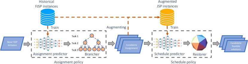
Figure 1: Two-stage Learning Framework for FJSP (2SL-FJSP)

Figure 1 presents 2SL-FJSP, the two-stage learning framework for the FJSP. Its various components and their contributions are explained in detail in this section. At a high level, 2SL-FJSP sequentializes the learning of assignment and scheduling decisions. Importantly, the first-stage assignment predictions are used through a branching process to generate instances used in the second-stage learning task, i.e., the predictions of the start times.

5.1 The Neural Network Structure

The parametric models used by 2SL-FJSP for predicting machine assignments and start times are inspired by the design proposed in Kotary et al. (2021a). The raw processing times $\mathbf{d}$ is split into two matrices: machine-task matrix $\mathbf{d}_{m}\in\mathbb{N}^{N\times M}$ and job-task matrix $\mathbf{d}_{j}\in\mathbb{N}^{N\times J}$, representing the machine-task structure and the job-task structure in FJSP. A distinct encoder is used on each matrix. The two encodings are then concatenated to form the inputs of a decoder that predicts the machine assignments or the start times.

$$\mathbf{h}_{m}=\text{Enc}_{\mathbf{\bm{\theta}}_{1}}(\mathbf{d}_{m}),$$

$$\mathbf{h}_{j}=\text{Enc}_{\mathbf{\bm{\theta}}_{2}}(\mathbf{d}_{j}),$$

$$\hat{\mathbf{y}}=\text{Dec}_{\mathbf{\bm{\theta}}_{3}}([\mathbf{h}_{j};\mathbf{h}_{2}]),$$

The encoders $\text{Enc}_{\mathbf{\bm{\theta}}_{1}}:\mathbb{N}^{N\times M}\rightarrow\mathbb{N}^{N\times H}$ and $\text{Enc}_{\mathbf{\bm{\theta}}_{2}}:\mathbb{N}^{N\times J}\rightarrow\mathbb{N}^{N\times H}$ are stacked 1-D convolution layers with $H$ filters. The decoder $\text{Dec}_{\mathbf{\bm{\theta}}_{3}}$ is a multi-layer perceptron that maps the flatted latent representation to the optimal decisions.

5.2 The Confidence-Aware Branching Scheme

The assignment predictions are not necessarily correct, which raises an interesting issue: the dataset of instances may not contain an instance with this particular (predicted) assignment. 2SL-FJSP addresses this challenge by using a confidence-aware branching scheme. The first element of the branching scheme is the parametruc model for the assignment predictions that is trained in a supervised learning fashion by minimizing the cross-entropy loss. The outputs $\hat{\mathbf{z}}$ for the machine-assignment layer are logits and they play a critical role to interface the assignment and scheduling policies. Given the logits $\mathbf{\hat{z}}\in\mathbb{R}^{N\times M}$ predicted by the deep learning model, the probability of a task $n$ being assigned to the machine $m$ is computed as:

$$p_{nm}=\frac{\exp(\hat{z}_{nm})\mathbb{I}\{d^{nm}\neq\infty\}}{\sum_{m^{\prime}\in[M]}\exp(\hat{z}_{nm^{\prime}})\mathbb{I}\{d^{nm^{\prime}}\neq\infty\}},$$ (5)

where $d^{nm}\neq\infty$ indicates task $n$ is compatible with machine $m$. The loss function $\mathcal{L}_{c}(\mathbf{p},\mathbf{z})$ of the first-stage predictive model is then defined as

$$-\sum_{\begin{subarray}{c}n,m\end{subarray}}z_{nm}\log{p}_{nm}+(1-z_{nm})\log(1-p_{nm})$$ (6)

To generate appropriate instances for training the scheduling policy, 2SL-FJSP uses confidence-aware branching, a strategy to generate a set of candidate assignments based on the confidence of the predictions. The candidate solutions are then used to generate the training data set for the scheduling policy. The confidence of the DNN prediction is based on the softmax function. More advanced uncertainty quantification such as MCDropout Gal and Ghahramani (2016) and deep ensembling Rahaman and others (2021) could be also used.

Confidence-aware branching borrows ideas from neighborhood search. It generates new candidate solutions by fixing the high-confidence predictions and perturbing the assignment predictions with lower confidence levels. More precisely, confidence-aware branching selects the subset $\mathcal{N}_{s}$ of tasks with the highest entropy, i.e.,

$$\mathcal{N}_{s}=\operatorname*{arg\,max}_{\mathcal{N}_{s}\in[N]}\sum_{n\in\mathcal{N}_{s}}\sum_{m\in[M]}-p_{nm}\log p_{nm},$$ (7)

and branches on all compatible assignments for every task $n\in\mathcal{N}_{s}$. The generated candidate assignments are used to augment the dataset for training the scheduling policies.

5.3 The Scheduling Policy

The scheduling policy of 2SL-FJSP is trained to imitate the CP solver. The loss function for its neural network minimizes a weighted sum of prediction errors and constraint violations, i.e.,

$$\mathcal{L}_{r}(\mathbf{s},\hat{\mathbf{s}},\mathbf{z},\mathbf{d})=\mathcal{L}(\mathbf{s},\hat{\mathbf{s}})+\lambda\sum_{c\in\mathcal{C}}v_{c}(\hat{\mathbf{s}},\mathbf{z},\mathbf{d}),$$ (8)

where $\hat{\mathbf{s}}$ denotes the predicted starting times, the function $\mathcal{L}(\mathbf{s},\hat{\mathbf{s}})=\|\mathbf{s}-\hat{\mathbf{s}}\|_{1}$ measures the distance of the predicted starting times with the optimal starting times, $v_{c}(\hat{\mathbf{s}},\mathbf{z},\mathbf{d})$ denotes the constraint violation of constraint $c$, and $\lambda$ denotes the coefficient of the constraint regularizer. Given the machine assignment $\mathbf{z}$ and the predicted starting times $\hat{\mathbf{s}}$, the job precedence constraint violation is computed as:

$$v_{1c}(\hat{s}_{jt}) =\max(0,\hat{s}_{jt}+d_{jt}^{m}-\hat{s}_{jt-1}).$$ (9)

The machine disjunctive constraint violation is given by:

$$v_{1d}(\hat{s}_{jt},\hat{s}_{j^{\prime}t^{\prime}})=\min(v_{1d}^{L}(\hat{s}_{jt},\hat{s}_{j^{\prime}t^{\prime}}),v_{1d}^{R}(\hat{s}_{jt},\hat{s}_{j^{\prime}t^{\prime}})),$$ (10)

with

$$v_{1d}^{L}(\hat{s}_{jt},\hat{s}_{j^{\prime}t^{\prime}})=\max(0,\hat{s}_{j^{\prime}t^{\prime}}+d_{j^{\prime}t^{\prime}}^{m}-\hat{s}_{jt}),$$

$$v_{1d}^{R}(\hat{s}_{jt},\hat{s}_{j^{\prime}t^{\prime}})=\max(0,\hat{s}_{jt}+d_{jt}^{m}-\hat{s}_{j^{\prime}t^{\prime}})$$

where $d^{m}_{ji}$ is the processing time on the assigned machine $m$ determined by the input assignment $\mathbf{z}$.

Although the constraint regularization pushes the predicted starting times into the feasible region, the predictions often violate some of the constraints. To restore feasibilty, the proposed learning framework uses the feasibility recovery in Kotary et al. (2021a) that runs in polynomial time. The details are deferred in Appendix B.

5.4 Symmetry-Breaking Data Generation

The last important contribution of 2SL-FJSP is a symmetry-breaking data generation that significantly facilitates the learning problem. The presence of symmetries in the FJSP raises additional difficulties for the learning task. Indeed, multiple identical machines can process the same job without affecting the makespan Ostrowski et al. (2010). In other words, given a feasible assignment solution $z$, multiple equivalent solutions can be obtained by permuting the columns of $z$. In optimization, symmetry-breaking techniques are often used to accelerate the search. However, different optimization instances may not break symmetry in the same way, leading to solutions that are quite distinct. This results in datasets that are harder to learn. In addition, for a complex problem like FJSP, it is not uncommon to generate sub-optimal solutions when optimal solutions cannot be obtained before the time limit. This poses another challenge for the learning task as different runs of the same, or similar, instances, may result in drastically different solutions. As a result, it is important to go beyond the standard approach that generates datasets by solving each instance independently.

2SL-FJSP features a novel symmetry-breaking data generation approach. The scheme is inspired by the approach proposed in Kotary et al. (2021a), but with an important difference. Instead of the sequential data generation framework that minimizes variations between consecutive ordered solutions, 2SL-FJSP uses a single reference point to break symmetries. As a result, 2SL-FJSP can solve all instances in parallel and all instances break symmetries the same way. Figure 2 illustrates the intuition behind the symmetry-breaking approach. In the figure, there are three co-optimal solutions from a standard FJSP perspective. The symmetry-breaking approach of 2SL-FJSP directs the search towards the solution that is closer to the pre-specified reference solution. Model 3 formalizes the symmetric-breaking scheme of 2SL-FJSP for the assignment policy. The idea is similar for the scheduling policy. In the model, $\hat{\textbf{z}}$ represents the reference assignment solution and $C_{max}^{*}$ is the optimal objective of the FJSP which is obtained in a first step. The objective (11a) minimizes the deviation of the optimal solution from a reference solution using the Hamming distance. Constraints (11b)-(11d) are the assignment, task-precedence, and machine constraints, respectively; they are identical to constraints (1c)-(1d). Constraint (11e) ensures that the quality of the symmetry-breaking solution is not worse than the optimal solution to the original FJSP. The experiments uses the CP formulation presented in Appendix C to solve Model 3.

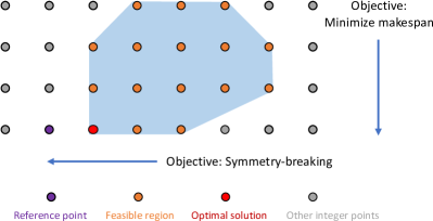
Figure 2: Illustration of the Symmetry-breaking Data Generation

Model 3 FJSP Symmetry Breaking Description

$$\mbox{Minimize}\quad\sum_{j,t,m}|z^{m}_{jt}-\hat{z}^{m}_{jt}|$$ (11a)

subject to:

$$\sum_{m\in M_{jt}}z^{m}_{jt}=1\qquad\forall j\in[J],t\in[T],$$ (11b)

$$s^{m}_{jt-1}\geq s^{i}_{j}+d^{m}_{jt}z^{m}_{jt}\qquad\forall j\in[J],t\in[T],t>0,m\in M_{jt},$$ (11c)

$$s^{m}_{jt}\geq s^{m}_{j^{\prime}t^{\prime}}+d^{m}_{j^{\prime}t^{\prime}}z^{m}_{j^{\prime}t^{\prime}}\quad\vee\quad s^{m}_{j^{\prime}t^{\prime}}\geq s^{m}_{jt}+d^{m}_{jt}z^{i}_{jt}$$ (11d)

$$\qquad\forall j,j^{\prime}\in[J],t,t^{\prime}\in[T],j\neq j^{\prime},m\in M_{jt},$$

$$C^{*}_{max}\leq s^{m}_{jt}+d^{m}_{jt}z^{m}_{jt}\;\qquad\forall(j,t)\in T,t=0,m\in M_{jt},$$ (11e)

$$z^{m}_{jt}\in\{0,1\}\qquad\forall j\in[J],t\in[T],m\in M_{jt}$$ (11f)

$$s^{m}_{jt}\geq 0\qquad\forall j\in[J],t\in[T],m\in M_{jt}$$ (11g)

6 Experimental Results

Table 1: Performances of models on FJSP instances. The best results are shown in bold. The relative optimality gap (Gap) is in percentage (%) and the solving time (Sol.T) is reported in second. The instances have sizes of the form ($J$ $\times$ $T$).

Method	Low flexibility										High flexibility
	car8 (8$\times$8)		mt10 (10$\times$10)		la22 (15$\times$10)		la32 (30$\times$10)		la40 (15$\times$15)		mt10 (10$\times$10)		la22 (15$\times$10)
	Gap	Sol. T	Gap	Sol. T	Gap	Sol. T	Gap	Sol. T	Gap	Sol. T	Gap	Sol. T	Gap	Sol. T
CP Solver	0.00	1.368	0.00	1.430	0.00	4.984	0.00	354.40	0.00	152.26	0.00	0.530	0.00	1315.0
2SL-FJSP	1.47	0.001	2.70	0.002	5.40	0.002	9.50	0.012	3.16	0.020	1.84	0.002	12.38	0.003
Encoder	0.26	0.001	6.04	0.002	15.48	0.002	12.71	0.012	12.68	0.020	7.29	0.002	28.11	0.003
DRL	25.18	0.594	28.55	0.779	26.34	1.394	27.26	2.459	26.88	1.769	61.43	0.083	63.94	0.145
FIFO_SPT	27.10	0.054	35.61	0.081	33.37	0.144	19.53	0.404	34.44	0.231	29.43	0.080	39.31	0.137
FIFO_EET	19.18	0.049	26.19	0.079	26.58	0.139	16.63	0.383	26.40	0.226	60.26	0.093	61.5	0.167
MOPNR_SPT	41.18	0.056	37.88	0.094	32.86	0.167	20.33	0.499	35.53	0.270	33.27	0.088	41.77	0.157
MOPNR_EET	41.78	0.053	35.98	0.090	30.17	0.159	20.87	0.461	33.32	0.257	89.69	0.087	106.38	0.150
LWKR_SPT	38.34	0.050	56.90	0.087	70.02	0.152	58.41	0.416	79.65	0.244	101.47	0.085	115.36	0.147
LWKR_EET	39.50	0.049	56.56	0.086	64.3	0.149	61.11	0.406	90.92	0.241	56.08	0.087	63.14	0.150
MWKR_SPT	34.81	0.051	30.50	0.086	20.12	0.150	17.65	0.419	35.43	0.243	29.47	0.084	39.94	0.146
MWKR_EET	32.03	0.050	26.93	0.085	15.38	0.148	17.48	0.414	31.04	0.240	41.29	0.776	57.71	1.163

Table 2: Optimality gap of ablated models. The best results are shown in bold. The relative optimality gap (Gap) is in percentage (%).

Method	Low flexibility					High flexibility
	car8	mt10	la22	la32	la40	mt10	la22
	8$\times$8	10$\times$10	15$\times$10	30$\times$10	15$\times$15	10$\times$10	15$\times$10
2SL-FJSP	1.47	2.70	5.40	9.50	3.16	1.84	12.38
2SL-FJSP (Branch)	1.64	3.36	6.39	10.49	3.39	1.91	19.44
2SL-FJSP (CR)	1.80	4.32	5.11	10.58	3.35	1.84	12.53
2SL-FJSP (SB)	8.04	6.32	15.40	15.23	6.83	5.23	18.23
2SL-FJSP (SB,CR)	8.87	7.52	16.23	16.43	7.21	5.43	19.81
Encoder	0.26	6.04	15.48	12.71	12.68	7.29	28.11
Encoder (SB)	4.70	10.21	16.88	15.32	12.06	18.23	38.12

Data Generation and Model Details

A single instance of the FJSP contains $J$ jobs and $M$ machines with a set of compatible assignments and the corresponding processing times for each task. Following Kotary et al. (2022), the instance generation simulates a situation when a scheduling system experiences an unexpected “slowdown” on some arbitrary machine, resulting in increased processing times of each task assigned to the impacted machine. To construct the dataset, a base instance is selected from the public benchmark Hurink et al. (1994) and a set of 20,000 individual problem instances are generated accordingly, with all the processing times on the impaired machine increased by up to 50 percent. Each FJSP instance is solved using IBM CP-Optimizer solver Laborie (2009) with a time limit of 1,800 seconds. For the JSP instances generated from the proposed branching policy, a maximum of 20,000 instances are randomly selected and solved to train the scheduling policy. The reference point for the symmetry-breaking scheme is the solution of the instance with 25% delay. The dataset is split in 8:1:1 for training, validation, and testing. All hyperparameter tunings are based on the validation metrics and all results are reported on the testing set. The deep learning models are implemented using PyTorch Imambi et al. (2021) and the training using Tesla V100 GPU on machines with Intel Xeon 2.7GHz and the Adam optimizer Kingma and Ba (2014). The hyperparameters were tuned using a grid search and their setting are detailed in Appendix D.

Baseline Methods

2SL-FJSP is compared with well-known rule-based heuristics from the literature. Like 2SL-FJSP, the heuristics are designed following a two-stage hierarchical scheme. The first stage involves a machine assignment rule, and the second stage involves a job sequencing rule. Many such rules have been proposed in the literature Jun et al. (2019). The experiments focus on eight heuristics that were shown to be effective (see Jun et al. (2019); Lei et al. (2022)). For machine selection, the experiments use the Smallest Processing Time (SPT) rule that assigns a machine with the smallest processing time of a task and the Earliest End Time (EET) rule that assigns a machine with the earliest end time of a task. For job sequencing, the experiments use the First in First out (FIFO) rule that processes a job that arrives the earliest at the queue of a machine, the Most Operation Number Remaining (MOPNR) rule that processes a job with the most number of tasks remaining, the Least Work Remaining (LWKR) rule that processes a job with the least work remaining, and the Most Work Remaining (WMKR) rule that processes a job with the most work remaining.

The experiments also compare 2SL-FJSP against the state-of-the-art CP commercial solver IBM CP-Optimizer Laborie (2009) and the state-of-the-art DRL method for FJSP Song et al. (2022). The DRL model is trained following the protocols defined in Song et al. (2022).

In addition, 2SL-FJSP is compared with weaker versions of itself in an ablation study:

• Encoder: a one-stage deep learning approach following the parameterization in Section 5.1 trained on the symmetry-breaking dataset to predict the assignment and start time,

• Encoder (SB): a one-stage deep learning approach trained on the dataset from standard data generation;

• 2SL-FJSP (Branch): 2SL-FJSP with no confidence-aware branching;

• 2SL-FJSP (SB): 2SL-FJSP trained on the dataset from standard data generation;

• 2SL-FJSP (CR): 2SL-FJSP trained on the dataset from symmetry-breaking data generation without constraint regularization;

• 2SL-FJSP (SB, CR): 2SL-FJSP trained on the dataset from standard data generation without constraint regularization.

6.1 Model Performance

Optimality Gap

The quality of the predictions is measured as a 1-shifted geometric mean of the relative difference between the makespan of the feasible solutions recovered from the predictions of the deep-learning models, and the makespan from the IBM CP solver with a time limit of 1,800s i.e., $\text{gap}=(\text{makespan}_{\text{model}}-\text{makespan}_{\text{cp}})/\text{makespan}_{\text{cp}}$. The optimality gap is the measure of the primary concern as the goal is to predict solutions of FJSP as close to the optimal as possible.

Table 1 reports the performance of the different models. First, 2SL-FJSP significantly outperforms all other baseline heuristics and the DRL method on all instances. The gap of 2SL-FJSP is up to an order of magnitude smaller than the results of the best heuristics on both low and high-flexibility instances. Similarly, 2SL-FJSP outperforms the one-stage deep learning approach except on car8, the smallest instance. This indicates that explicitly modeling the structure of FJSP facilitates learning. Interestingly, the DRL does not perform well on this set of test cases. A possible reason is that the DRL is trained on the dataset with a dramatic perturbation of jobs and machines in Song et al. (2022). This creates a distribution shift between the training environments and the test environments.

Solving Time

The solving times of different models are also reported in Table 1. For 2SL-FJSP and Encoder, the solving time includes the inference time and the solving time of the feasibility recovery. The feasibility recovery is modeled as a Linear Program (LP) and solved using Gurobi. In the experiments, all feasibility recovery finishes in milliseconds since the LPs are all solved in the presolving phase. 2SL-FJSP and Encoder are orders of magnitude faster than the CP solver and DRL, and even one order of magnitude faster than the fastest heuristics.

Ablation Study

To understand the benefits of the proposed components in 2SL-FJSP, Table 2 reports the results of weaker models with different components ablated. First, 2SL-FJSP models are always better than their one-stage counterparts Encoder except for the smallest instance car8. It indicates that explicitly modeling the hierarchical decisions helps the learning model better capture the structure of FJSP. Second, symmetry-breaking data generation shows great benefits for ML models. It significantly reduces the optimality gap of all instances, leading to up to 5 times smaller optimality gap for 2SL-FJSP and 20 times smaller optimality gap for Encoder. Finally, the confidence-aware branching and constraint regularization help reduce the optimality gap consistently for all instances except for the low flexibility la22.

7 Conclusion

This paper proposes 2SL-FJSP, a two-stage learning framework that delivers, in milliseconds, high quality solution for FJSP. It uses a confidence-aware branching scheme that enables generating appropriate instances to train scheduling decisions based on assignment predictions. The paper proposes a novel symmetry breaking formulation of FJSP to improve the performance of the learning task. This formulation allows solving instances in parallel contrary to previous work in this area that is primarily sequential in nature. Computational results show that 2SL-FJSP is capable of generating feasible FJSP solutions with quality that is significantly better than other approaches used in practice. This work is a first step towards enabling effective real-time decision making in the context of FJSP environments, especially those characterized with low and high flexibility levels. Future work includes improving the learning framework to accommodate, effectively, more complex settings such as fully-flexible job shop problems, where each task can be processed on any machine.

Appendix A FJSP CP formulation

A Constraint Programming (CP) formulation is proposed and used for solving FJSP. Two interval variables are used, $ops$ denoting a decision variable for each job $j$ and task $t$, and $mops$ denoting an optional decision variable for each job $j$ and its task $t$ on compatible machine $m$. Each interval variable has a domain $(s,e)$, where $s$ and $e$ are the start and end times of the interval, respectively, and $d=s-e$ is its length, in time units. The CP formulation is shown in Model 4 below. The objective (12a) minimizes the makespan. Constraints 12b, (12c), and 12d are the assignment, job precedence, and machine precedence constraints, respectively.

Model 4 A CP formulation for the FJSP

Minimizemax(end_of(ops[j,t]) for (j,t) in ops) (12a)

subject to:

$$\begin{split}\texttt{alternative(ops[j,t],[mops[j,t,m]:(j,t,m)}\in\texttt{mops]}\\ \forall\texttt{(j,t)}\in\texttt{ops},\end{split}$$ (12b)

$$\begin{split}\texttt{end\_before\_start(ops[j,t],ops[j,t-1])}\\ \forall\texttt{(j,t)}\in\texttt{ops,t>0},\end{split}$$ (12c)

$$\begin{split}\texttt{no\_overlap(mops[j,t,m] for (j,t,m)}\\ \forall\texttt{m}\in\texttt{M}.\end{split}$$ (12d)

Appendix B Feasibility Recovery

To recover feasibility, 2SL-FJSP utilizes a polynomial time procedure proposed in Kotary et al. [2022]. It relies on the fact that a predicted start time vector $\hat{s}$ implies an implicit task ordering between tasks assigned to the same machineModel 5 represents a linear programming (LP) formulation that finds the optimal schedule subject to such ordering. The objective function (13a) along with the job precedence constraints (13b) are identical to those of Model 2. Constraints (13c) reflects machine precedence constraints given task ordering, thus, eliminating the need for a disjunctive constraint set similar to that of Model 2. Using Model 5 was sufficient to restore feasibility in all of our experiments. However, it may happen that the resulting LP is infeasible as the machine precedence constraints may not be always consistent with the job precedence constraints. To address this, a greedy recovery algorithm can be used, as proposed in Kotary et al. [2022].

Model 5 LP formulation for feasibility recovery

$$\operatorname*{Minimize}\quad C_{max}$$ , (13a)

subject to:

$$\qquad s_{jt-1}\geq s_{jt}+d_{jt}\; \forall j\in[J],t\in[T],t>0,$$ (13b)

$$\qquad s_{jt}\geq s_{j^{\prime}t^{\prime}}+d_{j^{\prime}t^{\prime}} \forall j,j^{\prime}\in[J],t,t^{\prime}\in[T]:(j^{\prime},t^{\prime})\prec_{\hat{s}}(j,t),$$ (13c)

$$\qquad C_{max}\geq s_{jt}+d_{jt}\; \forall j\in[J],t\in[T],t=0,$$ (13d)

$$\qquad s_{jt}\geq 0 \forall j\in[J],t\in[T].$$ (13e)

Appendix C FJSP CP Symmetry Breaking formulation

A Constraint Programming (CP) formulation is proposed and used for solving the Symmetry Breaking version of FJSP. The description of decision variables and constraints is identical to that of the standard FJSP presented in Appendix A. The objective function (14a) is modified to minimize the deviation of the optimal solution from a reference solution. Constraints (14e) ensures that the quality of the symmetry-breaking solution is not worse than the optimal solution to the original FJSP.

Model 6 A Symmetry Breaking CP formulation for the FJSP

$$\begin{split}\texttt{Minimize}\qquad\texttt{sum(abs(presence\_of(mops[j,t,m]) - 1)}\\ \texttt{for (j,t,m)}\in\texttt{ref\_plan )}\end{split}$$ (14a)

subject to:

$$\begin{split}\texttt{end\_before\_start(ops[j,t],ops[j,t-1])}\\ \forall\texttt{(j,t)}\in\texttt{ops,t>0},\end{split}$$ (14b)

$$\begin{split}\texttt{alternative(ops[j,t],[mops[j,t,m]:(j,t,m)}\in\texttt{mops]}\\ \forall\texttt{(j,t)}\in\texttt{ops},\end{split}$$ (14c)

$$\begin{split}\texttt{no\_overlap(mops[j,t,m] for (j,t,m)}\\ \forall\texttt{m}\in\texttt{M},\end{split}$$ (14d)

$$\texttt{C}^{*}_{max}\geq\texttt{max(end\_of(ops[j,t]) for (j,t) in ops)}$$ (14e)

Appendix D Hyperparameters Tuning of Deep Learning Models

The following parameters were tuned given the following range for all neural network-based methods across all experiments:

• Maximum epochs: 1000

• Batch size: 32

• Encoding Layers: 2, 3

• Decoding Layers: 2, 3

• Dropout: 0.2

• Learning rate: 1e-1, 1e-2, 1e-3

In training, the learning rate is reduced to a factor of 10 if the validation metric does not improve for consecutive 10 epochs and the training early stops if the validation metric does not improve for consecutive 20 epochs. The hyperparameters of the model are selected by the smallest validation loss. The best hyperparameters of different models on different instances are reported in Table 3, 4, 5,6,7,8, respectively.

Table 3: The selected hyperparameters for car8 instances

dataset	model	lr	Enc. Layer	Dec. Layer
SB	2SL-FJSP (cls)	0.01	2	2
	2SL-FJSP (reg)	0.1	3	3
	Encoder (cls)	0.01	2	2
	Encoder (reg)	0.1	3	3
Standard	2SL-FJSP (cls)	0.1	2	2
	2SL-FJSP (reg)	0.01	2	2
	Encoder (cls)	0.1	2	2
	Encoder (reg)	0.01	2	2

Table 4: The selected hyperparameters for mt10 instances

dataset	model	lr	Enc. Layer	Dec. Layer
SB	2SL-FJSP (cls)	0.01	2	2
	2SL-FJSP (reg)	0.01	3	3
	Encoder (cls)	0.01	2	2
	Encoder (reg)	0.01	2	2
Standard	2SL-FJSP (cls)	0.01	2	2
	2SL-FJSP (reg)	0.01	3	3
	Encoder (cls)	0.01	2	2
	Encoder (reg)	0.01	2	2

Table 5: The selected hyperparameters for la22 instances

dataset	model	lr	Enc. Layer	Dec. Layer
SB	2SL-FJSP (cls)	0.01	2	2
	2SL-FJSP (reg)	0.001	2	2
	Encoder (cls)	0.01	2	2
	Encoder (reg)	0.1	3	3
Standard	2SL-FJSP (cls)	0.01	3	3
	2SL-FJSP (reg)	0.1	3	3
	Encoder (cls)	0.01	3	3
	Encoder (reg)	0.1	2	2

Table 6: The selected hyperparameters for la32 instances

dataset	model	lr	Enc. Layer	Dec. Layer
SB	2SL-FJSP (cls)	0.01	3	3
	2SL-FJSP (reg)	0.01	3	3
	Encoder (cls)	0.01	3	3
	Encoder (reg)	0.1	3	3
Standard	2SL-FJSP (cls)	0.01	3	3
	2SL-FJSP (reg)	0.01	3	3
	Encoder (cls)	0.01	2	2
	Encoder (reg)	0.1	3	3

Table 7: The selected hyperparameters for high flexible mt10 instances

dataset	model	lr	Enc. Layer	Dec. Layer
SB	2SL-FJSP (cls)	0.1	3	3
	2SL-FJSP (reg)	0.1	2	2
	Encoder (cls)	0.1	3	3
	Encoder (reg)	0.1	2	2
Standard	2SL-FJSP (cls)	0.1	3	3
	2SL-FJSP (reg)	0.1	2	2
	Encoder (cls)	0.1	3	3
	Encoder (reg)	0.1	2	2

Table 8: The selected hyperparameters for high flexible la22 instances

dataset	model	lr	Enc. Layer	Dec. Layer
SB	2SL-FJSP (cls)	0.1	3	3
	2SL-FJSP (reg)	0.01	3	3
	Encoder (cls)	0.1	3	3
	Encoder (reg)	0.01	2	2
Standard	2SL-FJSP (cls)	0.1	3	3
	2SL-FJSP (reg)	0.01	3	3
	Encoder (cls)	0.1	3	3
	Encoder (reg)	0.01	2	2

References

- Agrawal et al. [2019] Akshay Agrawal, Brandon Amos, Shane Barratt, Stephen Boyd, Steven Diamond, and J Zico Kolter. Differentiable convex optimization layers. Advances in neural information processing systems, 32, 2019.
- Amos and Kolter [2017] Brandon Amos and J Zico Kolter. Optnet: Differentiable optimization as a layer in neural networks. In International Conference on Machine Learning, pages 136–145. PMLR, 2017.
- Bengio et al. [2021] Yoshua Bengio, Andrea Lodi, and Antoine Prouvost. Machine learning for combinatorial optimization: a methodological tour d’horizon. European Journal of Operational Research, 290(2):405–421, 2021.
- Brandimarte [1993] Paolo Brandimarte. Routing and scheduling in a flexible job shop by tabu search. Annals of Operations research, 41(3):157–183, 1993.
- Chatzos et al. [2020] Minas Chatzos, Ferdinando Fioretto, Terrence WK Mak, and Pascal Van Hentenryck. High-fidelity machine learning approximations of large-scale optimal power flow. arXiv preprint arXiv:2006.16356, 2020.
- Chaudhry and Khan [2016] Imran Ali Chaudhry and Abid Ali Khan. A research survey: review of flexible job shop scheduling techniques. International Transactions in Operational Research, 23(3):551–591, 2016.
- Chen et al. [2020] Xinshi Chen, Yu Li, Ramzan Umarov, Xin Gao, and Le Song. Rna secondary structure prediction by learning unrolled algorithms. arXiv preprint arXiv:2002.05810, 2020.
- Donti et al. [2021] Priya L Donti, David Rolnick, and J Zico Kolter. Dc3: A learning method for optimization with hard constraints. arXiv preprint arXiv:2104.12225, 2021.
- Fattahi et al. [2007] Parviz Fattahi, Mohammad Saidi Mehrabad, and Fariborz Jolai. Mathematical modeling and heuristic approaches to flexible job shop scheduling problems. Journal of intelligent manufacturing, 18(3):331–342, 2007.
- Fioretto et al. [2020] Ferdinando Fioretto, Terrence WK Mak, and Pascal Van Hentenryck. Predicting ac optimal power flows: Combining deep learning and lagrangian dual methods. In Proceedings of the AAAI Conference on Artificial Intelligence, volume 34, pages 630–637, 2020.
- Gal and Ghahramani [2016] Yarin Gal and Zoubin Ghahramani. Dropout as a bayesian approximation: Representing model uncertainty in deep learning. In international conference on machine learning, pages 1050–1059. PMLR, 2016.
- Hurink et al. [1994] Johann Hurink, Bernd Jurisch, and Monika Thole. Tabu search for the job-shop scheduling problem with multi-purpose machines. Operations-Research-Spektrum, 15(4):205–215, 1994.
- Imambi et al. [2021] Sagar Imambi, Kolla Bhanu Prakash, and GR Kanagachidambaresan. Pytorch. In Programming with TensorFlow, pages 87–104. Springer, 2021.
- Jun et al. [2019] Sungbum Jun, Seokcheon Lee, and Hyonho Chun. Learning dispatching rules using random forest in flexible job shop scheduling problems. International Journal of Production Research, 57(10):3290–3310, 2019.
- Kawai and Fujimoto [2005] Tatsunobu Kawai and Yasutaka Fujimoto. An efficient combination of dispatch rules for job-shop scheduling problem. In INDIN’05. 2005 3rd IEEE International Conference on Industrial Informatics, 2005., pages 484–488. IEEE, 2005.
- Khalil et al. [2017] Elias Khalil, Hanjun Dai, Yuyu Zhang, Bistra Dilkina, and Le Song. Learning combinatorial optimization algorithms over graphs. Advances in neural information processing systems, 30, 2017.
- Kingma and Ba [2014] Diederik P Kingma and Jimmy Ba. Adam: A method for stochastic optimization. arXiv preprint arXiv:1412.6980, 2014.
- Kool et al. [2018] Wouter Kool, Herke Van Hoof, and Max Welling. Attention, learn to solve routing problems! arXiv preprint arXiv:1803.08475, 2018.
- Kotary et al. [2021a] James Kotary, Ferdinando Fioretto, and Pascal Van Hentenryck. Learning hard optimization problems: A data generation perspective. Advances in Neural Information Processing Systems, 34:24981–24992, 2021.
- Kotary et al. [2021b] James Kotary, Ferdinando Fioretto, Pascal Van Hentenryck, and Bryan Wilder. End-to-end constrained optimization learning: A survey. arXiv preprint arXiv:2103.16378, 2021.
- Kotary et al. [2022] James Kotary, Ferdinando Fioretto, and Pascal Van Hentenryck. Fast approximations for job shop scheduling: A lagrangian dual deep learning method. In Proceedings of the AAAI Conference on Artificial Intelligence, volume 36, pages 7239–7246, 2022.
- Laborie [2009] Philippe Laborie. Ibm ilog cp optimizer for detailed scheduling illustrated on three problems. In International Conference on Integration of Constraint Programming, Artificial Intelligence, and Operations Research, pages 148–162. Springer, 2009.
- Lei et al. [2022] Kun Lei, Peng Guo, Wenchao Zhao, Yi Wang, Linmao Qian, Xiangyin Meng, and Liansheng Tang. A multi-action deep reinforcement learning framework for flexible job-shop scheduling problem. Expert Systems with Applications, page 117796, 2022.
- Lin et al. [2019] Chun-Cheng Lin, Der-Jiunn Deng, Yen-Ling Chih, and Hsin-Ting Chiu. Smart manufacturing scheduling with edge computing using multiclass deep q network. IEEE Transactions on Industrial Informatics, 15(7):4276–4284, 2019.
- Liu et al. [2022] Renke Liu, Rajesh Piplani, and Carlos Toro. Deep reinforcement learning for dynamic scheduling of a flexible job shop. International Journal of Production Research, pages 1–21, 2022.
- Naderi and Roshanaei [2022] Bahman Naderi and Vahid Roshanaei. Critical-path-search logic-based benders decomposition approaches for flexible job shop scheduling. INFORMS Journal on Optimization, 4(1):1–28, 2022.
- Ostrowski et al. [2010] James Ostrowski, Miguel F Anjos, and Anthony Vannelli. Symmetry in scheduling problems. Citeseer, 2010.
- Park et al. [2019] In-Beom Park, Jaeseok Huh, Joongkyun Kim, and Jonghun Park. A reinforcement learning approach to robust scheduling of semiconductor manufacturing facilities. IEEE Transactions on Automation Science and Engineering, 17(3):1420–1431, 2019.
- Park et al. [2022] Seonho Park, Wenbo Chen, Dahye Han, Mathieu Tanneau, and Pascal Van Hentenryck. Confidence-aware graph neural networks for learning reliability assessment commitments. arXiv preprint arXiv:2211.15755, 2022.
- Rahaman and others [2021] Rahul Rahaman et al. Uncertainty quantification and deep ensembles. Advances in Neural Information Processing Systems, 34:20063–20075, 2021.
- Schulman et al. [2017] John Schulman, Filip Wolski, Prafulla Dhariwal, Alec Radford, and Oleg Klimov. Proximal policy optimization algorithms. arXiv preprint arXiv:1707.06347, 2017.
- Song et al. [2022] Wen Song, Xinyang Chen, Qiqiang Li, and Zhiguang Cao. Flexible job shop scheduling via graph neural network and deep reinforcement learning. IEEE Transactions on Industrial Informatics, 2022.
- Vesselinova et al. [2020] Natalia Vesselinova, Rebecca Steinert, Daniel F Perez-Ramirez, and Magnus Boman. Learning combinatorial optimization on graphs: A survey with applications to networking. IEEE Access, 8:120388–120416, 2020.
- Vinyals et al. [2015] Oriol Vinyals, Meire Fortunato, and Navdeep Jaitly. Pointer networks. Advances in neural information processing systems, 28, 2015.
- Vlastelica et al. [2019] Marin Vlastelica, Anselm Paulus, Vít Musil, Georg Martius, and Michal Rolínek. Differentiation of blackbox combinatorial solvers. arXiv preprint arXiv:1912.02175, 2019.
- Xie et al. [2019] Jin Xie, Liang Gao, Kunkun Peng, Xinyu Li, and Haoran Li. Review on flexible job shop scheduling. IET Collaborative Intelligent Manufacturing, 1(3):67–77, 2019.
- Zhang et al. [2020] Cong Zhang, Wen Song, Zhiguang Cao, Jie Zhang, Puay Siew Tan, and Xu Chi. Learning to dispatch for job shop scheduling via deep reinforcement learning. Advances in Neural Information Processing Systems, 33:1621–1632, 2020.