Flexible Modeling of Demographic Transition Processes with a Bayesian hierarchical penalized B-Splines model

Abstract

Several demographic and health indicators, including the total fertility rate (TFR) and modern contraceptive use rate (mCPR), exhibit similar patterns in their evolution over time, characterized by a transition between stable states. Existing statistical methods for estimation or projection are based on using parametric functions to model the transition. We introduce a more flexible model for transition processes based on B-splines called the B-spline Transition Model. We customize the model to estimate mCPR in 174 countries from 1970-2030 using data from the United Nations Population Division and validate performance with a set of out-of-sample model checks. While estimates and projections are comparable between the two approaches, we find the the B-spline approach improves out-of-sample predictions. Illustrative results for a model for TFR are also presented and show larger differences in projections when relaxing parametric assumptions.

T1This work was supported, in whole or in part, by the Bill & Melinda Gates Foundation (INV-00844). Under the grant conditions of the Foundation, a Creative Commons Attribution 4.0 Generic License has already been assigned to the Author Accepted Manuscript version that might arise from this submission.

and

1 Introduction

Projections of demographic and health indicators are of key interest for planning, to track progress towards international targets, or as inputs for projecting other outcomes of interest. For example, long-term projections of the Total Fertility Rate (TFR) to the year 2100 are produced by the United Nations for all countries in the world to provide insights into future outcomes (Alkema et al., 2011; Raftery, Alkema and Gerland, 2014; Liu and Raftery, 2020; United Nations, Department of Economic and Social Affairs, Population Division, 2022). In turn, these projections are used for constructing population projections (United Nations, Department of Economic and Social Affairs, Population Division, 2022), and population projections are subsequently used as input for other models, such as projecting warming due to climate change by 2100 (Raftery et al., 2017; Chen et al., 2022; Rennert et al., 2022). A second example is the projection of family planning indicators such as the modern contraceptive prevalence rate (mCPR) (Alkema et al., 2013; Cahill et al., 2018; Kantorová et al., 2020). Medium term projections of family planning indicators to the year 2030 are used to evaluate progress towards reaching the United Nations Sustainable Development Goals (Strong et al., 2020) and other targets, such as having 75% of demand for contraceptives satisfied by modern methods (Cahill, Weinberger and Alkema, 2020).

Transition models underlie the projections of a large set of demographic indicators. Transition models refer to models that capture transitions between stable states. Such models have been used to capture changes in indicators including the TFR and mCPR. For the TFR, this is the transition from high to low fertility referred to as the demographic transition (Kirk, 1996). The mCPR typically follows a transition from low availability and adoption of modern family planning methods to high availability and adoption. Other indicators for which transition models have been used to create projections include life expectancy (Raftery et al., 2013). These models have both been used by the international community for monitoring trends and generating projections in the indicator of interest.

Transition models aim to capture the relationship between the rate change of the indicator and its level for different populations. For example, for mCPR the rate of change starts slow at low levels of adoption, speeds up as modern methods become increasingly available, and then slows and eventually halts as demand is saturated (Alkema et al., 2013; Cahill et al., 2018). The Family Planning Estimation Model (FPEM) of Cahill et al. (2018) aims to capture this relation by positing that the rate of change in mCPR is related to its level by a logistic growth equation. The transition model used for projecting the TFR of Alkema et al. (2011) assumes a double logistic functional form for the relationship between rate of change and level of TFR. In both models, population-specific parameters are used to capture differences in the pace, timing, or stable states of transitions.

A limitation of these existing transition models is that an assumption is made that the rate versus level relationship for each indicator follows a particular functional form: a double logistic form, for TFR, and a logistic form, for mCPR. While additional model components are included to allow for deviations away from systematic trends, incorrect parametric forms may result in bias or incorrect coverage, in particular for longer term projections.

In this paper, we propose a new class of transition models in which the relation between rate of change and level is estimated flexibly, allowing for more data-adaptive estimation of transition functions as compared to existing approaches. Our proposed method, which we we refer to as a B-spline Transition Model (BTM), models the relationship between the rate of change of an indicator and its level using B-splines (de Boor, 1978; Eilers and Marx, 1996). Our approach allows for incorporating general prior knowledge on the shape of this relationship, such as monotonicity constraints, without having to specify a restrictive functional form. Rather, the specific shape of the relationship is learned from the available data, instead of being posited as a strong modeling assumption. The B-spline Transition model generalizes upon the current approaches used for projecting TFR and mCPR.

This paper is organized as follows. In Section 2 we introduce the mCPR case study. Section 3 introduces transition models and the B-spline Transition Model. We then propose a customized B-spline Transition Model in Section 4 to construct estimates and projections of mCPR in 174 UN countries. We validate the model through a set of out-of-sample model checks described in Section 5, using as a baseline for comparison a model based on the Family Planning Estimation Model (Cahill et al., 2018), the current model used for estimating mCPR by the United Nations (UN). Results for mCPR are presented in 6, and illustrative results for a B-spline Transition Model for TFR are given in 7. A discussion is included in Section 8.

2 Existing Approaches

In this section, we describe two existing models for mCPR and TFR. Each model makes strong functional form assumptions about the shape of the TFR and mCPR transitions, which motivates our proposed flexible modeling approach based on B-splines.

2.1 Modern Contraceptive Prevalence Rate: the Family Planning Estimation Model

As a case study, we consider the Modern Contraceptive Prevalence Rate (mCPR) indicator for married or in-union women, defined as the proportion of married or in-union women of reproductive age within a population who are using (or whose partner is using) a modern contraceptive method. The Family Planning Estimation Model (FPEM) is a Bayesian hierarchical model that has been used to generate projections of mCPR in countries (Alkema et al., 2013; Cahill et al., 2018).

Data on mCPR is typically derived from surveys in which participants report whether they or their partner are currently using a modern contraceptive method. Such surveys may be conducted by international organizations or by local organizations or governments. The UN Population Division has compiled a database of mCPR surveys in countries, subnational regions, and territories (United Nations 2021). We will refer to the geographic units included in the database generically as “countries”, although the data includes several subnational regions or territories. Data sources include the Demographic and Health Survey Program (DHS), Performance Monitoring for Action (PMA), UNICEF Multiple Indicator Cluster Surveys (MICS), and other national and international surveys. The UNPD preprocesses the microdata from each survey to yield country-level estimates of mCPR for the time period covered by the survey, taking into account the complex sampling design of each survey. The preprocessing may also yield a measure of the uncertainty in the mCPR estimate owed to the survey design, which we refer to as sampling error.

One of the primary challenges in modeling mCPR is posed by the wide range of data availability across countries. In the analysis dataset, availability ranged from a high of $n=34$ observations for Indonesia and a low of $n=1$ observations for $23$ areas. Figure 1 shows data for six areas, including 3 with relatively high availability (Bangladesh, Indonesia, Kenya) and 3 with relatively lower availability (Guinea, South Africa, Swaziland).

When data availability is high, we are able to see trends in the raw survey data that illustrate the temporal trends that are characteristic of a transition process in which mCPR transitions from between two stable states. In Bangladesh and Indonesia in particular there are sufficient data to see most of the transition from low to high mCPR (Figure 1). In Indonesia, a plateau in adoption can be seen, and in Bangladesh the data appear to follow a roughly S-shaped curve. In terms of the rate of change of mCPR vs. its level, in Bangladesh we can see that the rate of change is low at low levels, is larger at medium levels, and then becomes smaller again at higher levels as mCPR reaches an asymptote. Kenya provides an example of a country that does not appear to follow an S-shaped transition as neatly, as a temporary stall can be seen around the year 2000.

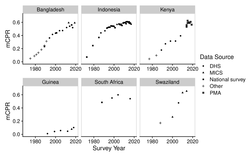
Figure 1: Observations of mCPR in countries with relatively high data availability (top row) vs. relatively low availability (bottom row).

FPEM draws on the observed S-shaped trend in the mCPR over time in its modeling approach. FPEM posits that the mCPR transition is given by a logistic growth equation. That is, it assumes that the rate of change of mCPR as a function of its level is given by a parametric function derived from a logistic growth equation. However, this logistic growth assumption at the core of FPEM may not always be justified. In particular, the symmetry of logistic growth implies that the pace of the contraceptive transition at the beginning of the transition is the same as at the end of the transition. Practically, this means that countries starting their transition are locked into a pace that carries forward into projections.

2.2 Total Fertility Rate: BayesTFR

The Total Fertility Rate (TFR) indicator is defined as the average number of children a woman in a specified population would have if she lives through all of her child-bearing years and experiences the corresponding age-specific fertility rates as she ages (Preston, Heuveline and Guillot, 2001). A Bayesian hierarchical model, BayesTFR, exists for estimating and projecting TFR in countries (Alkema et al., 2011; Raftery, Alkema and Gerland, 2014; Liu and Raftery, 2020; United Nations, Department of Economic and Social Affairs, Population Division, 2022).

The first step of BayesTFR is to apply a deterministic procedure to split the observed TFR time series data into three phases, corresponding to before (Phase I), during (Phase II), and after (Phase III) the demographic transition. BayesTFR applies different models to each phase as TFR is assumed to evolve differently depending on where a country is in the demographic transition. We will focus on the BayesTFR model for Phase II, as it is during this phase that TFR is expected to follow a transition from high to low. Figure 2 shows Phase II TFR estimates from six countries, using country estimates of TFR as obtained from the BayesTFR R package (Ševčíková, Alkema and Raftery, 2011), which (per October 2022) contains data from the 2019 edition of the United Nations World Population Prospects (United Nations, Department of Economic and Social Affairs, Population Division, 2019).

Figure 2: Total Fertility Rate (TFR) over time (5-year periods) in six selected countries.

BayesTFR models the transition (that is, the relationship between the rate of change and level of TFR) as following a double logistic function. Figure 3 shows the posterior distribution of the double logistic curves for Thailand and Kenya from BayesTFR, together with the decrements observed in the TFR estimates from Figure 2. The data from Thailand appear to be well fit by the model. In Kenya, however, the suitability of the logistic curves is less clear; observed rates of change suggest that decrements have increased in recent years, following a stall when the TFR was close to 6. This pattern cannot be captured by the double logistic function. This observation motivates our main contribution, which is to weaken the functional form assumption by modeling the transition using flexible modeling techniques.

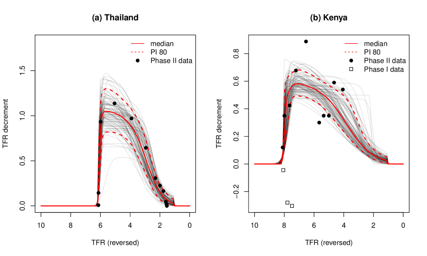
Figure 3: Fitted double logistic transition functions from the BayesTFR model plotted as the period-to-period decrement in TFR versus TFR. The black points show the empirical decrement vs. TFR. Note that the $x$-axis is reversed.

3 Transition Model

We begin by formalizing the inferential problem. Let $\eta_{c,t}\in\mathcal{E}$ be the true, latent value of an indicator in country $c$ at time $t$. The set $\mathcal{E}$ is left arbitrary for full generality; it is typically $(0,1)$ or $[0,1]$ for indicators that are proportions. We seek to estimate $\eta_{c,t}$ for countries $c=1,\dots,C$ and time points $t=1,\dots,T$ conditional on observations $y_{i}$, $i=1,\dots,n$, where $y_{i}$ is an observation of the indicator in country $c[i]$ and time $t[i]$.

Next, we introduce a model for indicators that are assumed to follow a transition process: that is, indicators assumed to follow a transition between two stable states, and where the rate of change is assumed to be a function of level. Following the framework of Temporal Models for Multiple Populations (TMMPs), we separate the model into a process model and a data model (Susmann, Alexander and Alkema, 2022). The process model defines the evolution of $\eta_{c,t}$ over time and the data model encodes the relationship between $\eta_{c,t}$ and observations $y_{i}$. In this section, we propose a process model based on estimating the relationship between rate and level with B-splines. Where applicable, we adopt the same notation as the TMMP model class.

Formally, the process model is given by

$$g_{1}(\eta_{c,t})=\begin{cases}\Omega_{c},&t=t^{*},\\ g_{1}(\eta_{c,t-1})+f(\eta_{c,t-1},\bm{\lambda}_{c},\bm{\beta}_{c})+\epsilon_{c,t},&t>t^{*},\\ g_{1}(\eta_{c,t+1})-f(\eta_{c,t+1},\bm{\lambda}_{c},\bm{\beta}_{c})-\epsilon_{c,t+1},&t<t^{*},\end{cases}$$ (1)

where $g_{1}:\mathcal{E}\to\mathbb{R}$ is a link function, $\Omega_{c}\in\mathbb{R}$ is the level of the indicator at a fixed reference year $t_{c}^{*}$, and $\epsilon_{c,t}$ is a residual. The function $f$ is a transition function depending on parameters $\bm{\lambda}_{c}\in\mathcal{E}^{2}$ and $\bm{\beta}_{c}\in\mathbb{R}^{p}$. The transition function $f$ predicts the rate of change of an indicator (on a possibly transformed scale, depending on $g_{1}$) as a function its level (on the original scale). The parameter vector $\bm{\lambda}_{c}=\{\lambda_{c}^{l},\lambda_{c}^{u}\}$, $\lambda_{c}^{u}>\lambda_{c}^{l}$, controls the asymptotes of the systematic component: that is, $\lambda_{c}^{l}$ is the minimum $\eta_{c,t}$ and $\lambda_{c}^{u}$ the maximum $\eta_{c,t}$ attainable through the systematic component. The parameter $\bm{\beta}_{c}$ controls the rate of the transition.

We introduce an additional constraint constraint that $f$ is either non-negative or non-positive; that is, $f(\eta,\bm{\lambda}_{c},\bm{\beta}_{c})\geq 0$ or $f(\eta,\bm{\lambda}_{c},\bm{\beta}_{c})\leq 0$ for all $\eta\in\mathcal{E}$. This constraint ensures that $g_{3}$ encodes a transition between two stable states. The manner in which $\eta_{c,t}$ moves between these two states will be determined by the particular form of $f$.

The deviations $\epsilon_{c,t}$ are intended to incorporate data-driven trends in the observed data that are not well captured by the systematic component. Typically a smoothing model is placed on the $\epsilon_{c,t}$ in order to avoid overfitting. The choice of smoothing model will likely depend on the indicator of interest, so the general class of transition models given by (1) does not make a-priori restrictions on $\epsilon_{c,t}$.

3.1 Logistic Transition Model: FPEM

One way of defining the transition function $f$ is to choose a particular parametric form. For example, if the transition is assumed to follow a logistic growth curve, starting at zero and reaching an asymptote $P_{c}^{u}$, then a logistic transition function $f_{l}$ can be chosen:

$$f_{l}(\eta_{c,t},\bm{\lambda}_{c},\bm{\beta}_{c})=\begin{cases}\mathrm{logit}\left(\lambda^{u}_{c}\cdot\mathrm{logit}^{-1}\left(\mathrm{logit}\left(\frac{\eta_{c,t}}{\lambda^{u}_{c}}\right)+\omega_{c}\right)\right)-\mathrm{logit}(\eta_{c,t}),&\eta_{c,t}<\lambda^{u}_{c}\\ 0,&\text{otherwise,}\end{cases}$$ (2)

where $\bm{\beta}_{c}=\{\omega_{c}\}$ for $\omega_{c}\geq 0$, the pace of the logistic curve. The form of $f_{l}$ can be derived algebraically as the rate of change on the logit scale of logistic growth as a function of level, and it can be seen that $f_{l}$ satisfies the non-negativity constraint. This form implies an asymptote in the transition when $\eta_{c,t}=\lambda_{c}^{u}$ and logistic growth when $\eta_{c,t}<\lambda^{u}_{c}$. An example logistic transition function is shown in Figure 4. The Family Planning Estimation Model (FPEM), an existing model for family planning indicators (including mCPR), is an example of a transition model that uses this logistic transition function (Cahill et al., 2018).

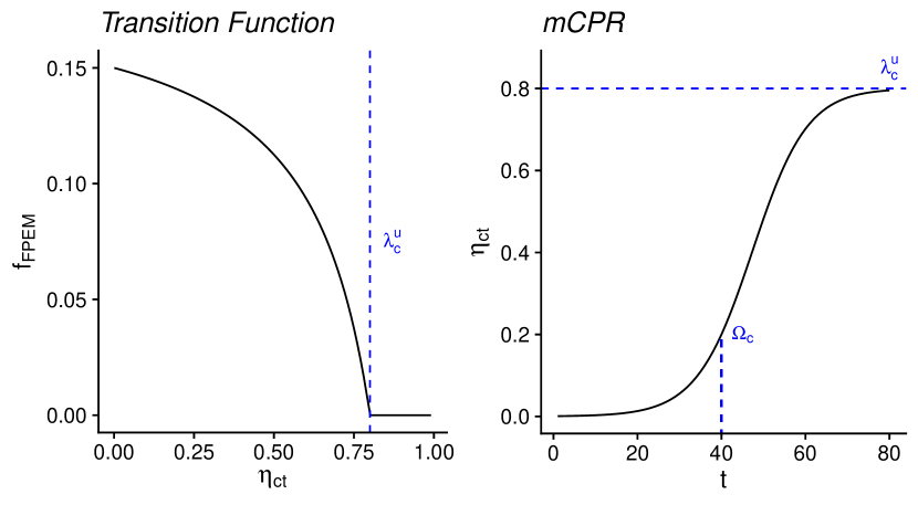
Figure 4: Left: an example of a logistic transition function $f_{l}$ for capturing a transition from zero to high mCPR $\eta_{c,t}$. Right: the evolution of $\eta_{c,t}$ over time that follows from the pictured transition function. The parameter $\Omega_{c}$ controls the level of the indicator at a reference time point and $P_{c}^{u}$ controls the asymptote.

3.2 Double Logistic Transition Model

The BayesTFR model provides a second example of a transition function defined by a specific functional form. Define a transition function $f_{dl}$ as

$$f_{dl}(\eta_{c,t},\bm{\lambda}_{c},\bm{\beta}_{c})= \begin{cases}\frac{-d_{c}}{1+\exp\left(-\frac{2\ln(9)}{\Delta_{c,1}}(\eta_{c,t}-\sum_{i}\Delta_{c,i}+0.5\Delta_{c,1})\right)}\\ \qquad+\frac{d_{c}}{1+\exp\left(-\frac{2\ln(9)}{\Delta_{c,3}}(\eta_{c,t}-\Delta_{c,4}-0.5\Delta_{c,3})\right)},&\eta_{c,t}>1,\\ 0,&\text{otherwise},\end{cases}$$ (3)

where $\bm{\beta}_{c}=\left\{d_{c},\Delta_{c,1},\Delta_{c,2},\Delta_{c,3},\Delta_{c,4}\right\}$. The parameter $d_{c}$ controls the maximum decrement in TFR during the transition, and the parameters $\Delta_{c,1},\dots,\Delta_{c,4}$ determine the shape of the double logistic curve. An example double logistic transition function is shown in Figure 5.

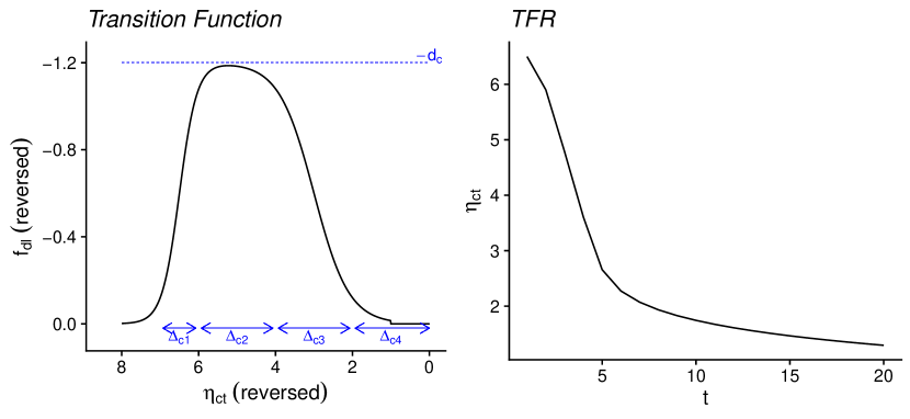
Figure 5: Left: an example of the double logistic transition function $f_{dl}$ for capturing a transition from high to low TFR $\eta_{c,t}$. Note that the $x$-axis and $y$-axis have been reversed, following convention. Right: the evolution of $\eta_{c,t}$ over time that follows from the pictured transition function.

3.3 B-spline Transition Model

Modeling $f$ using flexible modeling techniques allows capturing a wide variety of transitions. In this section we propose a flexible form for $f$ based on B-splines (de Boor, 1978; Eilers and Marx, 1996; Kharratzadeh, 2017). A B-spline function is defined by choosing a sequence $t_{1}<t_{2}<\cdots<t_{K}$ of knots and a spline degree $d$. Then the B-spline function is defined as a linear combination of basis functions $B_{d,j}(x)$, where $d$ is the basis degree and $j=1,\dots,K+d-1$. The basis functions are defined recursively, with $d=0$ yielding piecewise constant bases:

$$B_{0,j}(x)=\begin{cases}1,&t_{j}\leq x\leq t_{j+1},\\ 0,&\text{otherwise}.\end{cases}$$ (4)

Higher degree basis functions are defined recursively on an extended sequence of knots, in which $t_{1}$ is repeated $d$ times at the beginning of the sequence, and $t_{K}$ is repeated $d$ times at the end of the sequence. Then

$$B_{d,j}(x)=w_{d,j}B_{d-1,j}(x)+(1-w_{i+1,k})B_{d-1,j+1}(x),$$ (5)

where the weights are given by

$$w_{d,j}=\begin{cases}\frac{x-t_{j}}{t_{j+d-1}-t_{j}},&t_{j}\neq t_{j+d-1},\\ 0,&\text{otherwise.}\end{cases}$$ (6)

The smoothness of the B-spline function is controlled by the degree of basis functions (higher degrees yields a smoother functions) and the number of knots (fewer knots yields a smoother function). A degree $d=2$ is the smallest degree for which the spline function has first-order derivatives that exist everywhere, because $d=0$ leads to a piecewise constant function and $d=1$ leads to a piecewise linear function.

We define the B-spline transition function as

$$f_{b}(\eta_{c,t},\bm{\lambda}_{c},\bm{\beta}_{c})=\sum_{j=1}^{J}h_{j}(\beta_{c,j})B_{d,j}\left(\frac{\eta_{c,t}-\lambda_{c}^{l}}{\lambda_{c}^{u}-\lambda_{c}^{l}}\right),$$ (7)

where $B_{d,j}(\cdot)$ are spline basis functions as defined above, $h_{j}(\beta_{c,j})$ refers to the $j$th spline coefficient for area $c$, where $h_{j}:\mathbb{R}\to\mathbb{R}^{+}$ is a transformation of the parameter $\beta_{c,j}$, and parameters $\lambda_{c}^{l},\lambda_{c}^{u}\in\mathcal{E}$ are asymptote parameters that can be used to control the minimum and maximum $\eta_{c,t}$ attainable through the systematic component. The flexibility of $f_{b}$ can be tuned through the number of knots and the degree of the spline basis functions. The spline coefficients $\bm{\beta}_{c}$ control the shape of the transition function.

An example B-spline transition function is shown in Figure 6. For $f_{b}$ to be a well-defined transition function it is necessary that $f_{b}(\eta,\bm{\lambda}_{c},\bm{\beta}_{c})\geq 0$ (or $\leq 0$) for all $\eta\in\mathcal{E}$. This constraint can be satisfied through careful choice of the functions $h_{j}$. For example, it is sufficient to set $h_{j}(x)=\exp(x)$ for all $j$ to obtain $f_{b}(\eta,\bm{\lambda}_{c},\bm{\beta}_{c})\geq 0$.

If we set constraints on the spline coefficients such that $f_{b}$ is positive when $\eta_{c,t}/\lambda^{u}_{c}<1$ and zero when $\eta_{c,t}/\lambda^{u}_{c}\geq 1$ then the transition function dictates that the indicator will increase and have an asymptote at $\eta_{c,t}=\lambda_{c}^{u}$.

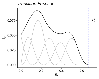
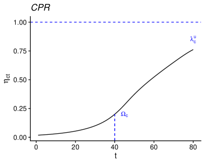
Figure 6: Left: an example of the B-spline transition function $f_{b}$ for capturing a transition from zero to high mCPR $\eta_{c,t}$. The gray lines illustrate a scaled version of the non-zero spline basis functions. Right: the evolution of $\eta_{c,t}$ over time that follows from the pictured transition function. The parameter $\Omega_{c}$ controls the level of the indicator at a reference time point, and the parameter $P_{c}$ controls the asymptote.

The logistic transition function $f_{l}$ (2) serves as a useful point of comparison to the B-spline transition function $f_{b}$. Because $f_{l}$ is monotonically decreasing, it cannot capture accelerations or stalls in the transition. In contrast, $f_{b}$ need not have such a monotonicity constraint, although one can be imposed if desired. In addition, a consequence of the logistic growth assumption is that the rate of change given by $f_{l}$ is symmetric around the midpoint of the transition. The B-spline function $f_{b}$, on the other hand, does not necessarily exhibit any such symmetry.

The B-spline transition function can be tailored to approximate any parametric transition function. To do so, the B-spline coefficients can be set in such a way that the resulting function $f_{b}$ approximates the parametric function. As such, any parametric transition function can be thought of as a special case of the B-spline transition function (in an approximate sense). In Appendix A we present the approximation of the logistic transition function with a B-spline representation.

3.3.1 Computation

We have developed subroutines in Stan (Stan Development Team, 2019; Gabry and Češnovar, 2021) that can be used as building blocks for implementing custom B-spline Transition Models. At its core is a custom B-spline implementation based on De Boor’s algorithm (de Boor, 1971). Sampling from the posterior distribution of model parameters is performed using Hamiltonian Markov Chain Monte-Carlo (MCMC) and the No-U-Turn sampler (Hoffman and Gelman, 2014). We synthesized our software into an open-source package for fitting B-spline Transition Models called BayesTransitionModels (https://github.com/AlkemaLab/BayesTransitionModels) implemented in the R programming language (R Core Team, 2022). An additional feature of the software is that hierarchical structures on model parameters $\bm{\lambda}_{c}$ and $\bm{\beta}_{c}$ can be easily incorporated. Additional R scripts for reproducing the results of this paper are available at https://github.com/herbps10/spline_rate_model_paper. The R package and reproduction code are also included in the Supplementary Material (Susmann and Alkema, 2022).

4 B-spline Transition Model for mCPR

In this section, we show how to apply our proposed modeling approach to build a transition model for mCPR. The description focuses on the process model. Information on the data and data model is given in section 4.3.

Let $\eta_{c,t}\in(0,1)$ be the true (latent) mCPR in country $c$ at time $t$, with countries and years indexed by $c=1,\dots,C$ and $t=1,\dots,T$. Let $s[c]$ index the subregion of area $c$ and $r[s]$ index the region of subregion $s$ (with $S$ total subregions and $R$ total regions).

The process model is given by the Transition Model (1), with the choice of transformation $g_{1}=\mathrm{logit}$ and the choice of the B-spline Transition Function $f_{b}$ yielding

$$\mathrm{logit}(\eta_{c,t})=\begin{cases}\Omega_{c},&t=t_{c}^{*},\\ \mathrm{logit}(\eta_{c,t-1})+f_{b}(\eta_{c,t-1},\bm{\lambda}_{c},\bm{\beta}_{c})+\epsilon_{c,t},&t>t_{c}^{*},\\ \mathrm{logit}(\eta_{c,t+1})-f_{b}(\eta_{c,t+1},\bm{\lambda}_{c},\bm{\beta}_{c})-\epsilon_{c,t+1},&t<t_{c}^{*}.\\ \end{cases}$$ (8)

and $f_{b}$ is defined as before (7). We chose $K$ knots of order $d$ such that the first $K-1$ knots are spaced evenly between $0$ and $1$ and the final knot is at $+\infty$ (for computation, it is set to $1000$). The reference year $t^{*}_{c}$ is set to 1990. Because we know that mCPR starts at zero in all countries, the parameter $\lambda_{c}^{l}$ is fixed to zero. The following additional constraints are introduced to ensure that $f_{b}$ is non-negative and induces an asymptote at $\lambda^{u}_{c}$

• The first $J-d-1$ coefficients are constrained to be positive. For computational reasons, we also constrain them to be greater than $0.01$ and less than $0.3$. As such, set

  $$h_{j}(x) =0.01+0.29\cdot\mathrm{logit}^{-1}(x),j=1,\dots,J-d-1.$$ (9)

  The upper bound is introduced only to improve the computational performance of the model, and are chosen such that the particular value of the bound is not informative of the model results.

• The final $d+1$ coefficients are constrained to be zero: $h_{J}(x)=h_{J-1}(x)=\cdots=h_{J-d}(x)=0$. This implies that $f_{b}(\eta,\bm{\lambda}_{c},\bm{\beta}_{c})=0$ for all $\eta\geq\lambda^{u}_{c}$ and that $f^{\prime}_{b}(x,\bm{\lambda}_{c},\bm{\beta}_{c})=0$.

Given these constraints, the parameter $\lambda^{u}_{c}$ can be interpreted as the upper asymptote of mCPR in country $c$. In other words, $\lambda^{u}_{c}$ is the highest value that $\eta_{c,t}$ can achieve solely through the systematic component. The lower bound on the first $J-d-1$ coefficients is introduced so that $\lambda^{u}_{c}$ is identifiable. Without a lower bound, spline coefficients at or near zero will induce an asymptote below $\lambda^{u}_{c}$ and $\lambda^{u}_{c}$ will not be well identified. An example of the B-spline transition function with the stated constraints is shown in Figure 6.

4.1 Hierarchical Models

Estimating the spline coefficients may be difficult in countries where little data are available. We make use of hierarchical models to share information on the shape of the transition function between countries, such that countries with few observations can borrow information from countries where more data are available. We follow the hierarchical structures used in Cahill et al. (2018).

The following hierarchical model is set on the spline coefficients $\beta_{c,j}$ for $j=1,\dots,J$:

$$\beta_{c,j}\mid\beta^{(r)}_{s[c],j},\sigma_{\beta,j}^{(c)} \sim N\left(\beta^{(s)}_{s[c],j},\left(\sigma_{\beta,j}^{(c)}\right)^{2}\right),$$ (10)

$$\beta^{(s)}_{s,j}\mid\beta^{(r)}_{r[s],j},\sigma_{\beta,j}^{(s)} \sim N\left(\beta^{(r)}_{r[s],j},\left(\sigma_{\beta,j}^{(s)}\right)^{2}\right),$$ (11)

$$\beta^{(r)}_{r,j}\mid\beta^{(w)}_{j},\sigma_{\beta,j}^{(r)} \sim N\left(\beta^{(w)}_{j},\left(\sigma_{\beta,j}^{(r)}\right)^{2}\right).$$ (12)

That is, the country-specific spline parameters $\beta_{c,j}$ are distributed around a subregion mean $\beta^{(s)}_{s[c],j}$, the subregion mean is distributed around a region mean $\beta^{(r)}_{r[s],j}$, and the regional mean is distributed around a world mean $\beta^{(w)}_{j}$. The standard deviations at the country, subregion, and region level are given by $\sigma^{(c)}_{\beta,j}$, $\sigma^{(s)}_{\beta,j}$, and $\sigma^{(r)}_{\beta,j}$. In this way, the hierarchical variance is allowed to differ for each coefficient. The following priors are set on the hyperparameters:

$$\sigma^{(c)}_{\beta,j} \sim N_{+}\left(0,0.5^{2}\right),$$ (13)

$$\sigma^{(s)}_{\beta,j} \sim N_{+}\left(0,0.5^{2}\right),$$ (14)

$$\sigma^{(r)}_{\beta,j} \sim N_{+}\left(0,0.5^{2}\right),$$ (15)

$$\beta^{(w)}_{j} \sim N\left(0,1\right),$$ (16)

where $j=1,\dots,J-d-1$.

In addition, a hierarchical model on $\lambda^{u}_{c}$ is used to share information about the mCPR asymptote between countries, with a transformation such that $\lambda_{c}$ is constrained to be between 0.5 and 0.95 (Cahill et al., 2018). Let

$$\lambda^{u}_{c}=0.5+0.45\cdot\mathrm{logit}^{-1}\left(\tilde{\lambda}^{u}_{c}\right),$$ (17)

where $\tilde{\lambda}^{u}_{c}\in\mathbb{R}$. Then a hierarchical model is applied to $\tilde{\lambda}^{u}_{c}$

$$\tilde{\lambda}^{u}_{c}\mid\tilde{\lambda}^{u,(w)},\sigma_{\tilde{\lambda}}^{(c)} \sim N\left(\tilde{\lambda}^{u,(w)},\left(\sigma^{(c)}_{\tilde{\lambda}^{u}}\right)^{2}\right),$$ (18)

such that $\tilde{\lambda}^{u}_{c}$ is distributed around a world mean $\tilde{\lambda}^{u,(w)}$ with standard deviation $\sigma_{\tilde{\lambda}}^{u,(c)}$. The hyperparameters were assigned the following priors:

$$\tilde{\lambda}^{u,(w)} \sim N\left(0,1\right),$$ (19)

$$\sigma^{(c)}_{\tilde{\lambda}^{u}} \sim N_{+}\left(0,1\right).$$ (20)

Finally, the parameter $\Omega_{c}$ gives the level of the process model at time $t=t_{c}^{*}$. To share information about the level of the indicator across countries, we assign $\Omega_{c}$ a hierarchical model such that $\Omega_{c}$ is distributed around a subregion, region, and world mean:

$$\Omega_{c}\mid\Omega^{(r)}_{s[c]},\sigma^{(c)}_{\Omega} \sim N\left(\Omega^{(r)}_{r[c]},(\sigma^{(c)}_{\Omega})^{2}\right),$$ (21)

$$\Omega^{(s)}_{s}\mid\Omega^{(r)}_{r[s]},\sigma^{(s)}_{\Omega} \sim N\left(\Omega^{(r)}_{r[s]},(\sigma^{(r)}_{\Omega})^{2}\right),$$ (22)

$$\Omega^{(r)}_{r}\mid\Omega^{(w)},\sigma^{(r)}_{\Omega} \sim N\left(\Omega^{(w)},(\sigma^{(r)}_{\Omega})^{2}\right).$$ (23)

The hyperparameters are given the following priors:

$$\Omega^{(w)} \sim N\left(0,1\right)$$ (24)

$$\sigma^{(c)}_{\Omega} \sim N_{+}\left(0,1\right),$$ (25)

$$\sigma^{(r)}_{\Omega} \sim N_{+}\left(0,1\right).$$ (26)

4.2 Smoothing Component

An AR(1) model is used to smooth the deviation terms $\epsilon_{c,t}$, with global autocorrelation parameter $\rho$ and variance parameter $\tau$:

_c,t $$\mid\rho,\tau\sim N\left(0,\rho^{2}/(1-\tau^{2})\right), t=t_{c}^{*},$$ (27)

$$\epsilon_{c,t} \mid\epsilon_{c,t-1},\rho,\tau\sim N\left(\rho\cdot\epsilon_{c,t-1},\tau^{2}\right), t>t_{c}^{*},$$ (28)

$$\epsilon_{c,t} \mid\epsilon_{c,t+1},\rho,\tau\sim N\left(\rho\cdot\epsilon_{c,t+1},\tau^{2}\right), t<t_{c}^{*}.$$ (29)

The hyperparameters are assigned the following priors:

$$\rho \sim\mathrm{Uniform}(0,1),$$ (30)

$$\tau \sim N_{+}(0,2^{2}).$$ (31)

4.3 Data and data Model

We use the UNPD data base to produce estimates of mCPR (United Nations, Department of Economic and Social Affairs, Population Division, 2021), available in the fpemlocal R package (Guranich et al., 2019). We apply several additional preprocessing steps to the UNPD database to construct an analysis dataset. We exclude two observations from the area “Other non-specified areas”. We also exclude $96$ observations marked in the database as exhibiting geographical region bias (e.g. the survey only sampled a subregion of the country) or bias related to measurement of modern method use. The analysis dataset after exclusions consisted of $n=1020$ observations. Because the Northern America region only includes The United States of America and Canada, it was combined with the Europe region. We impute sampling errors that are missing or reported as zero following the method described in (Cahill et al., 2018). Finally, although most surveys covered a period of one year or less, 31 observations covered a period of more than one year, including one that covered a period of approximately five years. We took the simplifying step of defining the survey year for each observation to be the midpoint of the start and end year, rounded down to the nearest year.

We define a simple data model. Let $y_{i}$ be the observed mCPR in country $c[i]$ and time $t[i]$ for $i=1,\dots,n$. Let $d[i]$ index the data source type of observation $i$ (with $D$ total data source types). Let $s_{i}^{2}$ be the fixed sampling variance for observation $i$. We adopt a truncated normal data model:

$$y_{i}\mid\eta_{c[i],t[i]},\sigma_{d[i]}\sim N_{[0,1]}(\eta_{c[i],t[i]},s_{i}^{2}+\sigma_{d[i]}^{2}),$$ (32)

where $\sigma_{d[i]}^{2}$ is a non-sampling error estimated for each data source type. The following prior is placed on the non-sampling error:

$$\sigma_{d}\sim N_{+}(0,0.1^{2}).$$ (33)

4.4 Comparison: Approximate Logistic Transition Model

We use a B-spline approximation of the logistic transition model as a baseline comparison model. The approximate logistic transition function is designed to follow the logistic transition function closely while still observing the constraint that the derivative of the spline function be zero at the asymptote $P_{c}$. We chose to approximate the logistic transition function using splines both for computational reasons, as the non-differentiability of the logistic transition function at $P_{c}$ can cause problems for gradient-based sampling algorithms such as Hamiltonian Markov Chain Monte-Carlo, and so that all parameters of the comparison model can be interpreted in the same way as the proposed model. Full details on the specification of the comparison model can be found in Appendix A (Section A).

5 Model Validation

In this section, we describe a set of out-of-sample model checks that can be used to evaluate the performance of a transition model, following those used to evaluate FPEM (Alkema et al., 2013). The model checks follow a similar structure which we describe here in the general case. Split the observations into a training set $\bm{y}^{\mathrm{train}}$ and validation set $\bm{y}^{\mathrm{val}}$. Fit the full model on $\bm{y}^{\mathrm{train}}$, yielding a set of posterior draws $\eta_{c,t}^{(\ell)}$ for $c=1,\dots,C$ and $t=1,\dots,T$, with $\ell$ indexing the draw. Compute the posterior predictive distribution for each of the held out data points, following the data model. That is, compute

$$\hat{y}^{(\ell)}_{i}\mid\eta_{c[i],t[i]}^{(\ell)},\sigma_{s[i]}^{(\ell)}\sim N_{[0,1]}(\eta_{c[i],t[i]}^{(\ell)},s_{i}^{2}+(\sigma^{(\ell)}_{d[i]})^{2})$$ (34)

for all $y_{i}\in\bm{y}^{\mathrm{val}}$. Let $\hat{y}_{i}^{q}$ be the empirical $q\%$ quantile of $\hat{y}_{i}^{(\ell)}$. Let $\bm{y}^{\mathrm{error}}\subset\bm{y}^{\mathrm{val}}$ be a subset of the held-out observations used for calculating coverage and error measures. We define the proportion included within the 95% uncertainty interval as

$$PPC=\frac{1}{|\bm{y}^{\mathrm{error}}|}\sum_{y_{i}\in\bm{y}^{\mathrm{error}}}\mathbb{I}[\hat{y}^{0.025}_{i}\leq y_{i}\leq\hat{y}^{0.975}_{i}].$$ (35)

We also compute the proportion of observations $y_{i}\in\bm{y}^{\mathrm{error}}$ that are below and above the 95% uncertainty interval given by $[\hat{y}^{0.025},\hat{y}^{0.975}]$, and the 95% credible interval width, given by $\hat{y}^{0.975}-\hat{y}^{0.025}$. Define the posterior predictive median error (ME) and median absolute error (MAE) as

$$ME =\mathrm{median}_{y_{i}\in\bm{y}^{\mathrm{error}}}\left\{\hat{y}^{0.5}_{i}-y_{i}\right\}$$ (36)

$$MAE =\mathrm{median}_{y_{i}\in\bm{y}^{\mathrm{error}}}\left\{|\hat{y}^{0.5}_{i}-y_{i}|\right\}.$$ (37)

Finally, to provide a more comprehensive view of uncertainty calibration beyond the 95% credible interval, we report the proportion of held-out observations falling below the $5\%$, $10\%$, $25\%$, and $50\%$ posterior quantiles, and the proportion of observations above the $50\%$, $75\%$, $90\%$, and $95\%$ posterior quantiles. These measures can be thought of as summarizing a Probability Integral Transform.

The observations are split into training and validation sets in two different ways, which are described below.

Exercise 1: Hold-out at random

The first validation is designed to evaluate the performance of the model when a subset of data are held-out at random. Choose $20\%$ of the observations at random for the validation set $\bm{y}^{\mathrm{val}}$. The remaining observations make up $\bm{y}^{\mathrm{train}}$. We use all of the held-out observations as long as there is at least one non-held-out observation within the same country for calculating the summary measures. This procedure is repeated 5 times and the summary measures averaged.

Exercise 2: Hold-out after cutoff year

The second validation is designed to evaluate the performance of the model in medium-term projections. First, let $L$ define a cutoff point, in years. Let $\bm{y}^{\mathrm{train}}=\{y_{i}:t[i]<L\}$, and $\bm{y}^{\mathrm{val}}=\{y_{i}:t[i]\geq L\}$. Countries that do not have any observations before the cutoff $L$ are not included in the summary measures. Because errors are likely to be correlated within countries, only the most recent held-out observation for each country is used to compute the validation measures.

6 mCPR Results

6.1 Computation

Tuning parameters differed for model validation runs and for a set of final models results. For model validations, 500 joint posterior distribution samples were drawn per chain from 4 chains after 250 warmup iterations. The max treedepth was set to $15$ and adapt delta to $0.999$. Based on the results of the model validations, two model configurations were chosen to generate a set of final results: the B-spline model with $d=2$, $K=5$ and the approximate logistic transition model. For the final results, the max treedepth was set to $14$, adapt delta to 0.999, and $750$ samples were drawn after $500$ warmup iterations, reflecting an increased emphasis on sampling accuracy.

Convergence of the MCMC algorithm was assessed with the improved split-chain $\hat{R}$ diagnostic and effective sample size (ESS) estimators described in Vehtari et al. (2021). For the final B-spline model ($d=2$, $K=5$), $\hat{R}$ for all parameters was between $0.999$ and $1.030$, all falling below the recommended threshold of $1.05$. The estimated bulk ESS ranged from $147$ to $10,431$. Finally, the diagnostics from the No-U-Turn sampler were optimal, with no divergent transitions and no transitions exceeding the maximum treedepth.

6.2 Validation Results

The model validations were conducted for several model specifications and tuning parameter values. For the base model specification, we tested every combination of spline degree $d=\{2,3\}$ and number of knots $K=\{5,7\}$ in order to investigate how the smoothness of the transition function effects model performance. As a comparison model, we used the approximate logistic transition model with $d=2$, $K=7$. Model Checks 1 and 2 are presented in Tables 1 and 2.

No single set of tuning parameters clearly outperforms the others (Table 1), although each either matches or beats the performance of the logistic comparison model. We are generally cautious to over-interpret the differences in validation measures between the models due to the relatively small number of held-out data points in the validation exercises, although some broad trends can be observed. A general pathology in all the models can be seen in their negative median errors in Model Check 2, suggesting they tend to over-predict mCPR in projections. However, the spline methods have median errors closer to zero than the comparison logistic model. Similarly, several of the base models have near-optimal empirical coverage of the 95% credible interval. However the points below and above the credible interval are not evenly balanced (Table 2). Again, the spline methods tend to perform similarly or better in this regard than the comparison, with the percent of observations falling below the ranging from $5.26\%$ to $6.77\%$ for the spline methods compared to $6.77\%$ for the comparison.

Based on the validation results, particularly in view of the similarity between the specifications, we chose to report substantive results from the base model specification with $d=2$, $K=5$.

	95% UI				Error
	% Below	% Included	% Above	CI Width	ME $\times 100$	MAE $\times 100$
				$\times 100$
Model Check 1
B-spline ($d=2$, $K=5$)	3.09%	93.2%	3.7%	20.1	-0.1870	2.79
B-spline ($d=2$, $K=7$)	3.33%	93.5%	3.13%	19.9	-0.1910	2.73
B-spline ($d=3$, $K=5$)	3.11%	93.4%	3.5%	20.2	-0.1560	2.89
B-spline ($d=3$, $K=7$)	1.92%	93.3%	4.81%	20.5	-0.0742	3.22
Logistic	3.09%	93.6%	3.3%	19.9	-0.1600	2.75
Model Check 2 ($L=2010$)
B-spline ($d=2$, $K=5$)	5.26%	93.2%	1.5%	32.1	-2.58	4.90
B-spline ($d=2$, $K=7$)	6.77%	92.5%	0.752%	32.1	-2.33	4.90
B-spline ($d=3$, $K=5$)	5.26%	94%	0.752%	32.6	-2.41	4.66
B-spline ($d=2$, $K=7$)	6.02%	92.5%	1.5%	32.0	-2.83	4.77
Logistic	6.77%	92.5%	0.752%	32.8	-3.28	4.86

Table 1: Validation results for Model Checks 1 and 2 summarizing the posterior predictive distribution of the held-out data points. The validation metrics are empirical coverage (% of held-out observations below, included, and above the 95% credible interval), 95% credible interval (CI) width, median error (ME), and median absolute error (MAE).

	$<5\%$	$<10\%$	$<25\%$	$<50\%$	$>50\%$	$>75\%$	$>90\%$	$>95\%$
Model Check 1
B-spline ($d=2$, $K=5$)	4.43%	9.06%	25.1%	52.1%	47.9%	20.6%	7.33%	4.83%
B-spline ($d=2$, $K=7$)	5.68%	9.66%	24.5%	52.6%	47.4%	20.2%	6.97%	4.63%
B-spline ($d=3$, $K=5$)	4.62%	9.07%	24.5%	52.3%	47.7%	22.3%	6.57%	4.46%
B-spline ($d=3$, $K=7$)	5.77%	10.6%	26%	51%	49%	22.1%	7.69%	4.81%
Logistic	6.16%	10%	25.1%	52.1%	47.9%	20.4%	6.76%	4.65%
Model Check 2 ($L$ = 2010)
B-spline ($d=2$, $K=5$)	8.27%	15%	35.3%	66.2%	33.8%	11.3%	3.76%	1.5%
B-spline ($d=2$, $K=7$)	9.02%	15%	33.8%	65.4%	34.6%	13.5%	3.76%	3.01%
B-spline ($d=3$, $K=5$)	7.52%	15%	33.8%	62.4%	37.6%	12%	3.76%	2.26%
B-spline ($d=2$, $K=7$)	9.02%	15%	36.1%	65.4%	34.6%	11.3%	3.76%	2.26%
Logistic	8.27%	15.8%	36.8%	69.9%	30.1%	9.77%	2.26%	1.5%

Table 2: Validation results for Model Checks 1-2 summarizing the properties of the posterior predictive distribution of held-out data points. Validation metrics are the % of held-out observations below the 5%, 10%, 25% and 50% posterior quantile and above the 50%, 75%, 80%, and 95% quantile.

6.3 mCPR Main Results

Posterior estimates of $\eta_{c,t}$ for the six selected countries of Figure 1, chosen to represent countries with high and low data availability, are shown in Figure 7. Results for all countries are included in the Supplementary Material (Susmann and Alkema, 2022). The estimates of $\eta_{c,t}$ tend to follow the observed data closely, although with added uncertainty derived from the non-sampling error term in the data model. The posterior distributions of the non-sampling error for each data source are summarized in Figure 8; PMA and DHS had the lowest estimated nonsampling error in terms of the posterior median, while MICS had the highest.

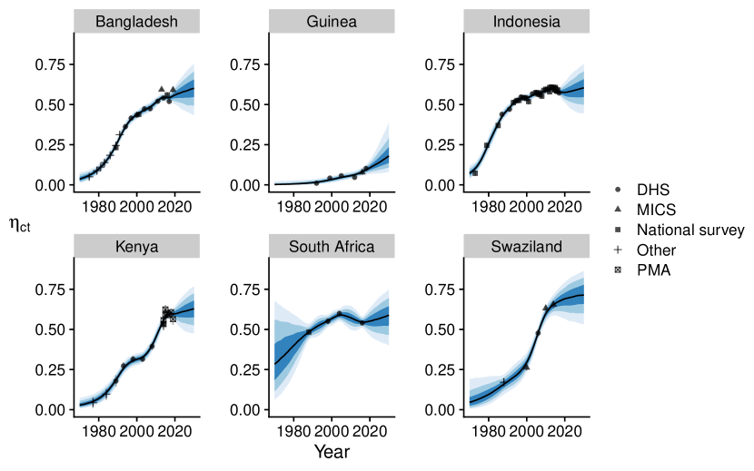
Figure 7: Posterior median (black line) and 50%, 80%, and 95% credible intervals (shaded regions) of $\eta_{c,t}$ (latent mCPR) in six countries from a B-spline Transition Model ($d=2$, $K=5$). The points show the observations, with vertical lines indicating the 95% confidence interval based on the sampling error.

Figure 8: Posterior median and 95% credibility interval for the non-sampling error parameters $\sigma_{s}^{2}$ for each data source.

The systematic and smoothing components of the process model interact to form the estimates of $\eta_{c,t}$ for each country. As an illustrative example, Figure 9 shows posterior estimates of the transition function, smoothing component, and $\eta_{c,t}$ for Kenya. The observed data from Kenya suggest that mCPR growth slowed around the year 2000. The transition function captures this by having a “double-peak” shape in which the rate of change is high, decreases in order to capture the stall, and then increases again to capture the observed increase in growth after the stall. The smoothing component also contributes to capturing the stall and subsequent increase, as the posterior median $\epsilon_{c,t}$ tends negative during the stall before turning positive.

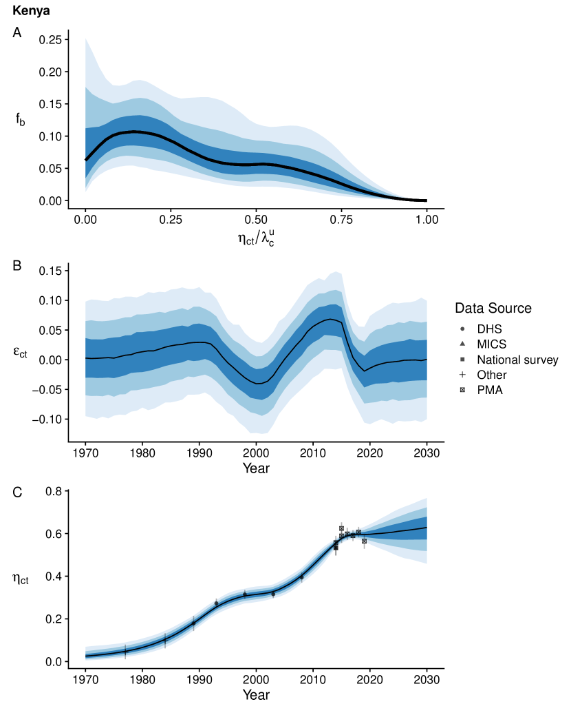
Figure 9: Posterior median (black lines) and 50%, 80%, and 95% credible intervals (shaded bands) of B-spline ($d=2,K=5$) model results from Kenya showing (A) transition function $f_{b}$, (B) smoothing component $\epsilon_{c,t}$, and (C) latent mCPR $\eta_{c,t}$. The points show the observations, with vertical lines indicating the 95% confidence interval based on the sampling error.

The shape of the transition function is informed by country-level data, when available, and by the transitions of other countries via the hierarchical model placed on the spline coefficients. Figure 10 illustrates the hierarchical distribution by showing the posterior median of the region, sub-region, and country-specific transition functions. The sub-regional transition function for Eastern Africa, for example, has a distinct “double-peak” shape, perhaps reflecting a slow-down in adoption in the 1990s and 2000s. The sub-regional transition function for Eastern Asia is quite different than for Asia as a whole, due in part to the steep increase in mCPR in China and the Republic of Korea from 1970 to 2000.

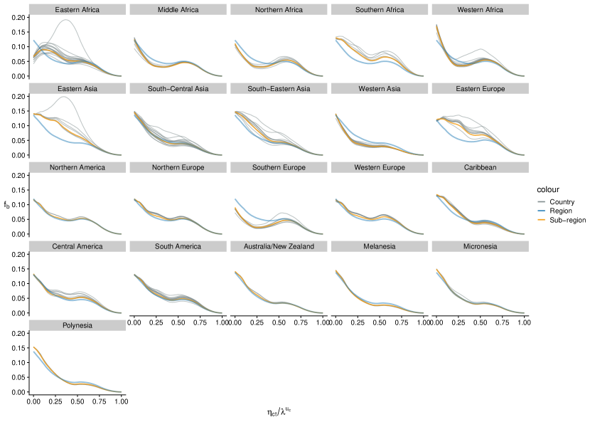
Figure 10: Posterior median transition functions $f_{b}$ for countries, sub-regions, and regions from the B-spline transition model ($d=2$, $K=5$).

Comparison with Logistic model

The added flexibility of the B-spline model relative to the logistic model leads to differences in estimates in some countries. Illustrative fits from the logistic model for the six selected countries are shown in Appendix Figure 17. The posterior estimates of mCPR in the year 2030 for the 15 countries with the largest absolute difference in posterior median between the B-spline and logistic models are shown in Figure 11. For all but three of these countries, the B-spline model is more conservative than the logistic model, projecting lower mCPR in 2030 (in terms of the posterior median).

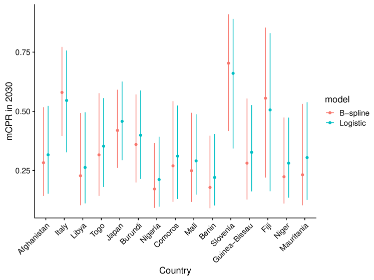
Figure 11: Posterior median and 95% credibility interval of $\eta_{c,2030}$ from the B-spline ($d=2$, $K=5$) and logistic models for the 15 countries where the absolute differences between the posterior median from each model are largest.

The smoothing components of the B-spline and logistic models also exhibit differences. To summarize the hyperparameters of the smoothing component, we calculated the unconditional standard deviation of $\epsilon_{c,t}$, given by $\tau/\sqrt{1-\rho^{2}}$. The posterior distribution for the unconditional standard deviation for the B-spline model is generally lower than that of the Logistic model (Figure 12). Rwanda provides an illustrative example of the difference in the smoothing component between the two models: the $\epsilon_{c,t}$ are smaller in the B-spline model because the sharp increase in adoption starting around 2005 can be in part captured by the more flexible B-spline transition function (Figure 13). However, the model estimates for $\eta_{c,t}$ for Rwanda are remarkably similar between the two models, suggesting that the added uncertainty from allowing the transition function to be more flexible balances the lower variance in the smoothing component.

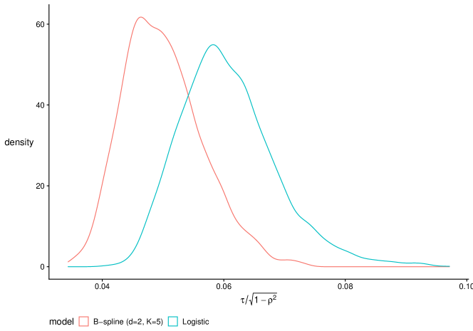
Figure 12: Posterior distribution of $\tau/\sqrt{1-\rho^{2}}$, the unconditional standard deviation of the smoothing component, for the B-spline ($d=2$, $K=5$) and Logistic models.

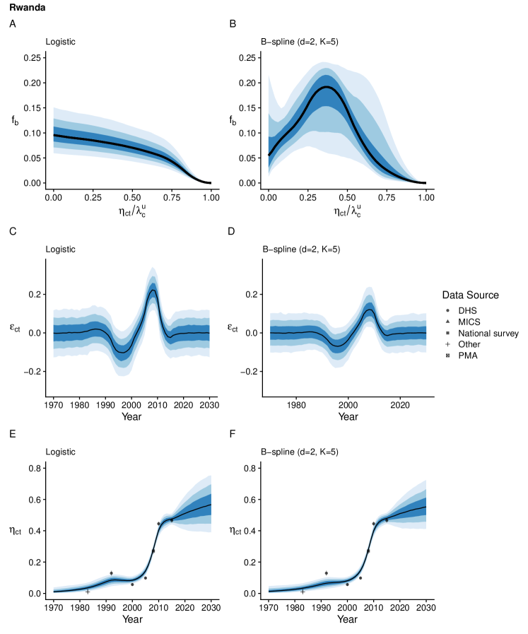
Figure 13: Posterior median (black lines) and 50%, 80%, and 95% credible intervals (shaded bands) of (A, B) transition functions $f_{b}$ for the logistic and B-spline ($d=2,K=5$) models, (C, D) smoothing component $\epsilon_{c,t}$, and (E, F) latent mCPR $\eta_{c,t}$. The points show the observations, with vertical lines indicating the 95% confidence interval based on the sampling error.

7 Illustrative TFR Results

In this section, we present illustrative results from the B-spline Transition Model applied to estimating and projecting TFR. The B-spline Transition Model specification for TFR is given in Appendix D.

7.1 Computation

The model was fit with $K=7$ knots and spline degree $d=2$. The MCMC algorithm was run for $500$ iterations after $500$ warmup iterations. The max treedepth was set to $12$ and the adapt delta tuning parameter to $0.999$. No transitions were divergent or exceeded the maximum treedepth. The $\hat{R}$ for all parameters was between 0.998 and 1.022, and the bulk ESS was between $221$ and $4781$.

7.1.1 Results

We compare our results to a modified version of BayesTFR that generates projections only using the Phase II model. This is done to highlight the long-term behavior of the B-spline and double logistic transition models in projections. However, we emphasize that both the BayesTFR and B-spline results presented here are therefore not comparable to published projections from the full BayesTFR model and should be interpreted solely in the context of understanding the possible benefits and drawbacks of the proposed B-spline transition model for Phase II estimation. In addition, more research is needed to validate the choice of priors and spline hyperparameters for the B-spline transition model for TFR.

The estimated transition functions are shown in Figure 14. In several countries we can see that the added flexibility of the B-splines allows the transition function to fit the observed declines in TFR more closely. This is particularly true in the Congo and Cameroon, where the splines follow slowdowns in TFR declines more closely than the double logistic functions. The resulting transition functions as estimated by the spline model are more variable than those from BayesTFR. The spline transition functions for all of the pictured countries include the possibility of larger declines in TFR than is found in the double logistic fits.

The posterior distribution of $\eta_{c,t}$ with projections to the 2095-2100 5-year period for the same six countries is shown in Figure 15. The associated transition functions for each country are shown in Figure 14. The B-spline based projections generally exhibit higher uncertainty than those based on the double logistic functions, which is not surprising given the additional flexibility of the splines. The median spline projections for Angola, Cameroon, and Congo are lower than those from the double logistic transition, reflecting how the spline transition functions include the possibility of larger declines. In Chad, the median projections are remarkably similar, although the spline projections exhibit higher uncertainty.

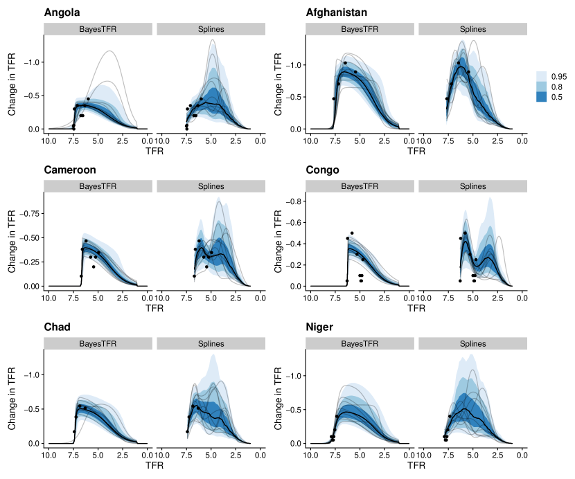
Figure 14: Estimated transition functions from the BayesTFR and B-spline Transition Model for TFR giving the estimated rate of change in TFR versus level of TFR. Black lines are posterior medians, and shaded regions show 50%, 80%, and 95% credibility intervals. A sample of 10 draws from the posterior distribution of the transition functions are shown as gray lines. The points show the observed declines in TFR as a function of TFR.

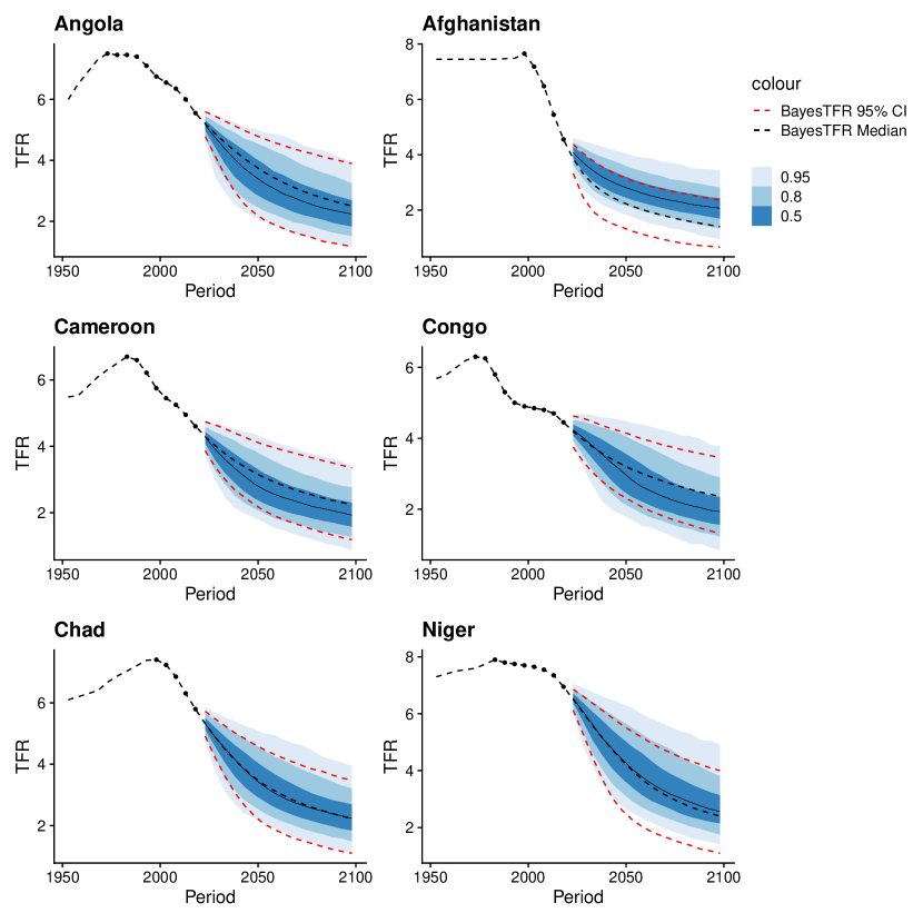
Figure 15: Posterior projections of the TFR from the BayesTFR and B-spline Transition Model for TFR. The black dotted line shows the BayesTFR posterior median, and the red dotted line the BayesTFR 95% credibility interval. The shaded regions show the 50%, 80%, and 95% credibility intervals from the B-spline Transition Model. Note that estimation is performed for $5$-year intervals. The continuous lines on the plot are meant only to aid the eye and should not be interpreted as yearly estimates.

8 Discussion

The B-spline Transition Model proposed in this paper demonstrates that it is possible to estimate and project demographic and health indicators using flexible estimation techniques that eschew strong functional form assumptions. Using mCPR as our main application, we found it is possible to substantially weaken assumptions on the shape of the relationship between the rate of change and level of an indicator without sacrificing out-of-sample predictive performance. Our illustrative results for the TFR demonstrate that the B-spline Transition Model can be considered more generally for projecting indicators that follow transition processes.

In addition to providing a flexible estimation approach, our model also yields a novel way to summarize and communicate trends in indicators through the estimated shape of the transition functions. For example, in our mCPR case study, the regional and sub-regional transition functions, derived from the hierarchical distribution placed on the spline coefficients reveals systematic differences in the transitions between groups of countries.

Substantively, in our applications, we found that projections from the B-spline model were often similar to those from more parameterized models. Despite the added flexibility inherent in the B-spline Transition Model, in many countries the mCPR estimates of $\eta_{c,t}$ are quite similar to the comparison Logistic model. This could be seen as evidence that the logistic assumption made by earlier models is a sound one. The similarities may also reflect the data-sparse setting in the case-study, in which models of a similar structure may converge on similar results because they reach the limit of what is possible to infer given the limited data. For TFR projections, we did obtain outcomes that differed more substantially between the spline and double-logistic models. Additional research is needed to assess in more detail the performance of the B-spline model for projecting the TFR.

The B-spline transition model can be extended to capture more complex behaviors. For example, a transition function that is allowed to vary over time would allow the systematic component to fit temporal trends in the transition. For example, the mCPR indicator in some subregions appears to have gone through a slowdown in the 1990s and 2000. In our current model, this is captured in the shape of the (time-invariant) transition functions and by the smoothing component. However, if there is a shared, temporally localized slowdown then it may be more effective to explicitly capture it via a time-varying transition function. In addition, analyzing the posterior summaries of the time-varying transition functions would provide another method to summarize and communicate trends in mCPR, such as regional or subregional slowdowns in adoption. Finally, while the focus of this article is to propose a flexible estimation strategy for the transition function, an alternative specification for the smoothing term may also yield benefits.

The B-spline Transition Model is a flexible model for indicators that follow transition processes and is extendable to capture trends exhibited by other indicators. As interest in generating estimates and projections of health indicators grows, the B-Spline Transition Model provides a useful framework for developing models that relax strong functional form assumptions in favor of learning relationships from the data.

Appendix A Approximate Logistic Transition Function

This appendix describes an approximation of the logistic transition function using the B-spline transition function. To enforce the logistic growth assumption within our model framework, we introduce a new set of constraints on the first $J-3$ spline coefficients. Let $x^{*}_{j}=\operatorname*{\arg\,\max}_{x\in[0,1]}B_{j}(x)$ be the point at which the $j$th spline basis function is maximized. Set $\beta_{c,j}=l(x^{*}_{j},\lambda^{u}_{c},\omega_{c})$ for $j=1,\dots,J-3$, where the parameter $\omega_{c}$ is a pace parameter controlling the rate of the logistic growth curve and $l(x,\lambda^{u},\omega)=((x-\lambda^{u})\omega)/(\lambda^{u}(x-1))$ gives the rate of change for logistic growth for a level $x$, upper asymptote $\lambda^{u}$, and pace parameter $\omega$.

Figure 16 shows an example B-spline transition function with this constraint applied. The difference between the approximation and the true $f_{\textrm{FPEM}}$ is caused by the constraint inherited from the B-spline setup that the transition function must have a derivative of zero at the asymptote.

We place a hierarchical model on $\omega_{c}$ to share information between countries, nested within subregion, region, and world. Let

$$\omega_{c}=0.5\cdot\mathrm{logit}^{-1}(\tilde{\omega}_{c}),$$ (38)

for $\tilde{\omega}_{c}\in\mathbb{R}$ such that $\omega_{c}$ is constrained to be between $0$ and $0.5$. We use the following hierarchical model:

$$\tilde{\omega}_{c}\mid\tilde{\omega}^{(s)}_{s[c]},\sigma^{(c)}_{\tilde{\omega}} \sim N\left(\tilde{\omega}^{(s)}_{s[c]},\left(\sigma^{(c)}_{\tilde{\omega}}\right)^{2}\right),$$ (39)

$$\tilde{\omega}^{(s)}_{s}\mid\tilde{\omega}^{(s)}_{r[s]},\sigma^{(s)}_{\tilde{\omega}} \sim N\left(\tilde{\omega}^{(r)}_{r[s]},\left(\sigma^{(s)}_{\tilde{\omega}}\right)^{2}\right),$$ (40)

$$\tilde{\omega}^{(r)}_{r}\mid\tilde{\omega}^{(w)},\sigma^{(r)}_{\tilde{\omega}} \sim N\left(\tilde{\omega}^{(w)},\left(\sigma^{(r)}_{\tilde{\omega}}\right)^{2}\right).$$ (41)

The hyperparameters are assigned the following priors:

$$\sigma^{(c)}_{\tilde{\omega}} \sim N_{+}\left(0,1\right),$$ (42)

$$\sigma^{(s)}_{\tilde{\omega}} \sim N_{+}\left(0,1\right),$$ (43)

$$\sigma^{(r)}_{\tilde{\omega}} \sim N_{+}\left(0,1\right),$$ (44)

$$\tilde{\omega}^{(w)} \sim N\left(0,1\right).$$ (45)

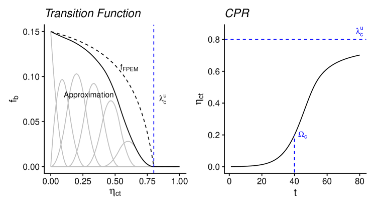
Figure 16: Left: an example of a constrained B-spline transition function $f_{b}$ for the approximate logistic transition model. The gray lines illustrate a scaled version of the non-zero spline basis functions. Right: the curve implied by the pictured transition function.

Appendix B Extended mCPR Validation Results

Tables 3 and 4 show the results for Model Check $3$.

	95% UI				Error
	% Below	% Included	% Above	CI Width	ME $\times 100$	MAE $\times 100$
				$\times 100$
Model Check 3 ($L=2015$)
B-spline ($d=2$, $K=5$)	5.05%	92.9%	2.02%	24.0	-1.16	3.65
B-spline ($d=2$, $K=7$)	6.06%	91.9%	2.02%	23.8	-1.33	3.72
B-spline ($d=3$, $K=5$)	6.06%	91.9%	2.02%	24.3	-1.52	3.79
B-spline ($d=2$, $K=7$)	6.06%	91.9%	2.02%	24.1	-1.46	3.60
Logistic	5.05%	93.9%	1.01%	25.0	-2.11	3.11

Table 3: Validation results for Model Check 3 summarizing the posterior predictive distribution of the held-out data points. The validation metrics are empirical coverage (% of held-out observations below, included, and above the 95% credible interval), 95% credible interval (CI) width, median error (ME), and median absolute error (MAE).

	$<5\%$	$<10\%$	$<25\%$	$<50\%$	$>50\%$	$>75\%$	$>90\%$	$>95\%$
Model Check 3 ($L$ = 2015)
B-spline ($d=2$, $K=5$)	7.07%	12.1%	31.3%	61.6%	38.4%	12.1%	5.05%	2.02%
B-spline ($d=2$, $K=7$)	7.07%	14.1%	31.3%	60.6%	39.4%	15.2%	5.05%	2.02%
B-spline ($d=3$, $K=5$)	7.07%	13.1%	31.3%	61.6%	38.4%	15.2%	5.05%	2.02%
B-spline ($d=2$, $K=7$)	7.07%	14.1%	32.3%	63.6%	36.4%	13.1%	5.05%	2.02%
Logistic	7.07%	12.1%	33.3%	65.7%	34.3%	7.07%	3.03%	2.02%

Table 4: Validation results for Model Check 3 summarizing the properties of the posterior predictive distribution of held-out data points. Validation metrics are the % of held-out observations below the 5%, 10%, 25% and 50% posterior quantile and above the 50%, 75%, 80%, and 95% quantile.

Appendix C Additional Results

Figure 17 illustrates several model fits from the logistic approximation to the B-spline Transition Model.

Figure 17: Posterior median (black line) and 50%, 80%, and 95% credible intervals (shaded regions) of $\eta_{c,t}$ (latent mCPR) in six countries from the logistic approximation to the B-spline Transition Model. The points show the observations, with vertical lines indicating the 95% confidence interval based on the sampling error.

Appendix D B-spline Transition Model for TFR

We implemented a B-splines transition model for projecting TFR. Model specifications related to the use of data and the phases associated with the TFR transitions followed those made by (Alkema et al., 2011). Let $\eta_{c,t}\in\mathbb{R}^{+}$ be the true (latent) TFR in country $c$ at time period $t$, with countries and time periods indexed by $c=1,\dots,C$ and $t=1,\dots,T$. As per Alkema et al. (2011) specifications, United Nations Population Division (UNPD) TFR estimates are assumed to equal the true TFR.

The process model is given by

$$\eta_{c,t}=\begin{cases}\Omega_{c},&t=t_{c}^{*},\\ \eta_{c,t-1}+f_{b}(\eta_{c,t-1},\bm{\lambda}_{c},\bm{\beta}_{c})+\epsilon_{c,t},&t>t_{c}^{*},\\ \eta_{c,t+1}-f_{b}(\eta_{c,t+1},\bm{\lambda}_{c},\bm{\beta}_{c})-\epsilon_{c,t+1},&t<t_{c}^{*},\\ \end{cases}$$ (46)

The reference year $t_{c}^{*}$ is set to the first time point of Phase II in country $c$, and the parameter $\Omega_{c}$ is fixed to the value of the first observed data point in Phase II. The upper asymptote is set to $\lambda^{u}_{c}=\Omega_{c}$ and the lower to $\lambda^{l}_{c}=1$. That is, the transition is assumed to start at the level of the first data point in Phase II and is lower bounded by a TFR of 1.

We chose $K$ dots of order $d$ such that the first knot is at $-\infty$ and the remaining $K-1$ knots are spaced evenly between 0 and 1. Additional constraints are added such that $f_{b}$ is negative and $f_{b}(0,\bm{\lambda}_{c},\bm{\beta}_{c})=0$:

• The first $d+1$ coefficients are constrained to be zero: $h_{0}(x),\dots,h_{d+1}(x)=0$ and $h_{J-d-1}(x),\dots,h_{J}(x)=0$.

• The middle $J-d-1$ coefficients are constrained to be between $-0.01$ and $-2.49$:

  $$h_{j}(x)=-0.01-2.49\cdot\mathrm{logit}(x),j=d+1,\dots,J$$ (47)

These constraints encode the assumption that the demographic transition is from high to low TFR, and that the rate of change of TFR should approach zero smoothly when TFR approaches one.

Aligned with BayesTFR, a hierarchical model is applied to the transition parameters $\bm{\beta}_{c}$ such that information on the rate and shape of the transition is shared between countries:

$$\beta_{c,j}\mid\beta^{(r)}_{s[c],j},\sigma_{\beta,j}^{(c)} \sim N\left(\beta^{(w)}_{j},\left(\sigma_{\beta,j}^{(c)}\right)^{2}\right).$$

That is, each $\beta_{c,j}$, $j=1,\dots,J$ is normally distributed around a world mean $\beta_{j}^{(w)}$ with standard deviation $\sigma_{\beta,j}^{(c)}$. The following priors are used for the hyperparameters:

$$\sigma^{(c)}_{\beta,j} \sim N_{+}\left(0,1\right),$$

$$\beta^{(w)}_{j} \sim N\left(0,1\right),$$

where $j=d,\dots,J-d-1$.

Again aligned with BayesTFR, a white noise smoothing model is assumed:

$$\epsilon_{c,t}\sim N(0,\tau),$$ (48)

where $\tau$ is given the prior $\tau\sim N_{+}(0,1)$.

This work was supported, in whole or in part, by the Bill & Melinda Gates Foundation (INV-00844). Under the grant conditions of the Foundation, a Creative Commons Attribution 4.0 Generic License has already been assigned to the Author Accepted Manuscript version that might arise from this submission

Estimates and projections of mCPR for all countries B-spline transition model estimates and projections of mCPR for all countries in the analysis dataset.

R package and reproduction code Source code of the BayesTransitionModel R package and code for reproducing the paper’s results: urlhttps://github.com/AlkemaLab/BayesTransitionModels and https://github.com/herbps10/spline_rate_model_paper.

Supplementary Material: Estimates and projections of mCPR for all countries

Model fits for all countries from the B-spline transition model for mCPR ($d=2$, $K=5$) are presented below.

See pages 1- of figures/spline_results.pdf

References

- Alkema et al. (2011) {barticle}[author] \bauthor\bsnmAlkema, \bfnmLeontine\binitsL., \bauthor\bsnmRaftery, \bfnmAdrian E\binitsA. E., \bauthor\bsnmGerland, \bfnmPatrick\binitsP., \bauthor\bsnmClark, \bfnmSamuel J\binitsS. J., \bauthor\bsnmPelletier, \bfnmFrançois\binitsF., \bauthor\bsnmBuettner, \bfnmThomas\binitsT. and \bauthor\bsnmHeilig, \bfnmGerhard K\binitsG. K. (\byear2011). \btitleProbabilistic projections of the total fertility rate for all countries. \bjournalDemography \bvolume48 \bpages815–839. \bdoi10.1007/s13524-011-0040-5 \endbibitem
- Alkema et al. (2013) {barticle}[author] \bauthor\bsnmAlkema, \bfnmLeontine\binitsL., \bauthor\bsnmKantorova, \bfnmVladimira\binitsV., \bauthor\bsnmMenozzi, \bfnmClare\binitsC. and \bauthor\bsnmBiddlecom, \bfnmAnn\binitsA. (\byear2013). \btitleNational, regional, and global rates and trends in contraceptive prevalence and unmet need for family planning between 1990 and 2015: a systematic and comprehensive analysis. \bjournalThe Lancet \bvolume381 \bpages1642–1652. \bdoi10.1016/S0140-6736(12)62204-1 \endbibitem
- Cahill, Weinberger and Alkema (2020) {barticle}[author] \bauthor\bsnmCahill, \bfnmN\binitsN., \bauthor\bsnmWeinberger, \bfnmM\binitsM. and \bauthor\bsnmAlkema, \bfnmL\binitsL. (\byear2020). \btitleWhat increase in modern contraceptive use is needed in FP2020 countries to reach 75% demand satisfied by 2030? An assessment using the Accelerated Transition Method and Family Planning Estimation Model [version 1; peer review: 2 approved]. \bjournalGates Open Research \bvolume4. \bdoi10.12688/gatesopenres.13125.1 \endbibitem
- Cahill et al. (2018) {barticle}[author] \bauthor\bsnmCahill, \bfnmNiamh\binitsN., \bauthor\bsnmSonneveldt, \bfnmEmily\binitsE., \bauthor\bsnmStover, \bfnmJohn\binitsJ., \bauthor\bsnmWeinberger, \bfnmMichelle\binitsM., \bauthor\bsnmWilliamson, \bfnmJessica\binitsJ., \bauthor\bsnmWei, \bfnmChuchu\binitsC., \bauthor\bsnmBrown, \bfnmWin\binitsW. and \bauthor\bsnmAlkema, \bfnmLeontine\binitsL. (\byear2018). \btitleModern contraceptive use, unmet need, and demand satisfied among women of reproductive age who are married or in a union in the focus countries of the Family Planning 2020 initiative: a systematic analysis using the Family Planning Estimation Tool. \bjournalThe Lancet \bvolume391 \bpages870–882. \bdoi10.1016/S0140-6736(17)33104-5 \endbibitem
- Chen et al. (2022) {barticle}[author] \bauthor\bsnmChen, \bfnmXin\binitsX., \bauthor\bsnmRaftery, \bfnmAdrian E.\binitsA. E., \bauthor\bsnmBattisti, \bfnmDavid S.\binitsD. S. and \bauthor\bsnmLiu, \bfnmPeiran R.\binitsP. R. (\byear2022). \btitleLong-term probabilistic temperature projections for all locations. \bjournalClimate Dynamics. \bdoi10.1007/s00382-022-06441-8 \endbibitem
- de Boor (1971) {btechreport}[author] \bauthor\bparticlede \bsnmBoor, \bfnmCarl\binitsC. (\byear1971). \btitleSubroutine package for calculating with B-splines. \btypeTechnical Report No. \bnumberLA-4728-MS, \bpublisherLos Alamos National Lab, Los Alamos, NM. \endbibitem
- de Boor (1978) {bbook}[author] \bauthor\bparticlede \bsnmBoor, \bfnmCarl\binitsC. (\byear1978). \btitleA practical guide to splines. \bpublisherSpringer, \baddressNew York, NY. \endbibitem
- Eilers and Marx (1996) {barticle}[author] \bauthor\bsnmEilers, \bfnmPaul H. C.\binitsP. H. C. and \bauthor\bsnmMarx, \bfnmBrian D.\binitsB. D. (\byear1996). \btitleFlexible smoothing with B-splines and penalties. \bjournalStatistical Science \bvolume11 \bpages89 – 121. \bdoi10.1214/ss/1038425655 \endbibitem
- Gabry and Češnovar (2021) {bmanual}[author] \bauthor\bsnmGabry, \bfnmJonah\binitsJ. and \bauthor\bsnmČešnovar, \bfnmRok\binitsR. (\byear2021). \btitlecmdstanr: R Interface to ’CmdStan’ \bnotehttps://mc-stan.org/cmdstanr, https://discourse.mc-stan.org. \endbibitem
- Guranich et al. (2019) {bmanual}[author] \bauthor\bsnmGuranich, \bfnmGregory\binitsG., \bauthor\bsnmWheldon, \bfnmMark\binitsM., \bauthor\bsnmCahill, \bfnmNiamh\binitsN. and \bauthor\bsnmAlkema, \bfnmLeontine\binitsL. (\byear2019). \btitlefpemlocal: fpemlocal \bnoteR package version 1.0.2. \endbibitem
- Hoffman and Gelman (2014) {barticle}[author] \bauthor\bsnmHoffman, \bfnmMatthew D.\binitsM. D. and \bauthor\bsnmGelman, \bfnmAndrew\binitsA. (\byear2014). \btitleThe No-U-Turn Sampler: Adaptively Setting Path Lengths in Hamiltonian Monte Carlo. \bjournalJournal of Machine Learning Research \bvolume15 \bpages1593–1623. \endbibitem
- Kantorová et al. (2020) {barticle}[author] \bauthor\bsnmKantorová, \bfnmVladimíra\binitsV., \bauthor\bsnmWheldon, \bfnmMark C.\binitsM. C., \bauthor\bsnmUeffing, \bfnmPhilipp\binitsP. and \bauthor\bsnmDasgupta, \bfnmAisha N. Z.\binitsA. N. Z. (\byear2020). \btitleEstimating progress towards meeting women’s contraceptive needs in 185 countries: a Bayesian hierarchical modelling study. \bjournalPLOS Medicine \bvolume17 \bpages1–23. \bdoi10.1371/journal.pmed.1003026 \endbibitem
- Kharratzadeh (2017) {barticle}[author] \bauthor\bsnmKharratzadeh, \bfnmMilad\binitsM. (\byear2017). \btitleSplines in Stan. \bjournalStan Case Studies, Volume 4. \endbibitem
- Kirk (1996) {barticle}[author] \bauthor\bsnmKirk, \bfnmDudley\binitsD. (\byear1996). \btitleDemographic Transition Theory. \bjournalPopulation Studies \bvolume50 \bpages361-387. \bnotePMID: 11618374. \bdoi10.1080/0032472031000149536 \endbibitem
- Liu and Raftery (2020) {barticle}[author] \bauthor\bsnmLiu, \bfnmPeiran\binitsP. and \bauthor\bsnmRaftery, \bfnmAdrian E.\binitsA. E. (\byear2020). \btitleAccounting for uncertainty about past values in probabilistic projections of the total fertility rate for most countries. \bjournalThe Annals of Applied Statistics \bvolume14 \bpages685 – 705. \bdoi10.1214/19-AOAS1294 \endbibitem
- Preston, Heuveline and Guillot (2001) {bbook}[author] \bauthor\bsnmPreston, \bfnmSamuel H\binitsS. H., \bauthor\bsnmHeuveline, \bfnmPatrick\binitsP. and \bauthor\bsnmGuillot, \bfnmMichel\binitsM. (\byear2001). \btitleDemography: Measuring and Modeling Population Processes. \bpublisherBlackwell Publishing Ltd, \baddressOxford, UK. \endbibitem
- Raftery, Alkema and Gerland (2014) {barticle}[author] \bauthor\bsnmRaftery, \bfnmAdrian E.\binitsA. E., \bauthor\bsnmAlkema, \bfnmLeontine\binitsL. and \bauthor\bsnmGerland, \bfnmPatrick\binitsP. (\byear2014). \btitleBayesian Population Projections for the United Nations. \bjournalStatistical Science \bvolume29 \bpages58 – 68. \bdoi10.1214/13-STS419 \endbibitem
- Raftery et al. (2013) {barticle}[author] \bauthor\bsnmRaftery, \bfnmAdrian E\binitsA. E., \bauthor\bsnmChunn, \bfnmJennifer L\binitsJ. L., \bauthor\bsnmGerland, \bfnmPatrick\binitsP. and \bauthor\bsnmSevčíková, \bfnmHana\binitsH. (\byear2013). \btitleBayesian probabilistic projections of life expectancy for all countries. \bjournalDemography \bvolume50 \bpages777–801. \bdoi10.1007/s13524-012-0193-x \endbibitem
- Raftery et al. (2017) {barticle}[author] \bauthor\bsnmRaftery, \bfnmAdrian E.\binitsA. E., \bauthor\bsnmZimmer, \bfnmAlec\binitsA., \bauthor\bsnmFrierson, \bfnmDargan M. W.\binitsD. M. W., \bauthor\bsnmStartz, \bfnmRichard\binitsR. and \bauthor\bsnmLiu, \bfnmPeiran\binitsP. (\byear2017). \btitleLess than 2 C warming by 2100 unlikely. \bjournalNature Climate Change \bvolume7 \bpages637–641. \bdoi10.1038/nclimate3352 \endbibitem
- Rennert et al. (2022) {barticle}[author] \bauthor\bsnmRennert, \bfnmKevin\binitsK., \bauthor\bsnmErrickson, \bfnmFrank\binitsF., \bauthor\bsnmPrest, \bfnmBrian C.\binitsB. C., \bauthor\bsnmRennels, \bfnmLisa\binitsL., \bauthor\bsnmNewell, \bfnmRichard G.\binitsR. G., \bauthor\bsnmPizer, \bfnmWilliam\binitsW., \bauthor\bsnmKingdon, \bfnmCora\binitsC., \bauthor\bsnmWingenroth, \bfnmJordan\binitsJ., \bauthor\bsnmCooke, \bfnmRoger\binitsR., \bauthor\bsnmParthum, \bfnmBryan\binitsB., \bauthor\bsnmSmith, \bfnmDavid\binitsD., \bauthor\bsnmCromar, \bfnmKevin\binitsK., \bauthor\bsnmDiaz, \bfnmDelavane\binitsD., \bauthor\bsnmMoore, \bfnmFrances C.\binitsF. C., \bauthor\bsnmMüller, \bfnmUlrich K.\binitsU. K., \bauthor\bsnmPlevin, \bfnmRichard J.\binitsR. J., \bauthor\bsnmRaftery, \bfnmAdrian E.\binitsA. E., \bauthor\bsnmŠevčíková, \bfnmHana\binitsH., \bauthor\bsnmSheets, \bfnmHannah\binitsH., \bauthor\bsnmStock, \bfnmJames H.\binitsJ. H., \bauthor\bsnmTan, \bfnmTammy\binitsT., \bauthor\bsnmWatson, \bfnmMark\binitsM., \bauthor\bsnmWong, \bfnmTony E.\binitsT. E. and \bauthor\bsnmAnthoff, \bfnmDavid\binitsD. (\byear2022). \btitleComprehensive evidence implies a higher social cost of CO2. \bjournalNature \bvolume610 \bpages687–692. \bdoi10.1038/s41586-022-05224-9 \endbibitem
- Strong et al. (2020) {barticle}[author] \bauthor\bsnmStrong, \bfnmKathleen\binitsK., \bauthor\bsnmNoor, \bfnmAbdislan\binitsA., \bauthor\bsnmAponte, \bfnmJohn\binitsJ., \bauthor\bsnmBanerjee, \bfnmAnshu\binitsA., \bauthor\bsnmCibulskis, \bfnmRichard\binitsR., \bauthor\bsnmDiaz, \bfnmTheresa\binitsT., \bauthor\bsnmGhys, \bfnmPeter\binitsP., \bauthor\bsnmGlaziou, \bfnmPhilippe\binitsP., \bauthor\bsnmHereward, \bfnmMark\binitsM., \bauthor\bsnmHug, \bfnmLucia\binitsL., \bauthor\bsnmKantorova, \bfnmVladimira\binitsV., \bauthor\bsnmMahy, \bfnmMary\binitsM., \bauthor\bsnmMoller, \bfnmAnn-Beth\binitsA.-B., \bauthor\bsnmRequejo, \bfnmJennifer\binitsJ., \bauthor\bsnmRiley, \bfnmLeanne\binitsL., \bauthor\bsnmSay, \bfnmLale\binitsL. and \bauthor\bsnmYou, \bfnmDanzhen\binitsD. (\byear2020). \btitleMonitoring the status of selected health related sustainable development goals: methods and projections to 2030. \bjournalGlobal Health Action \bvolume13 \bpages1846903. \bnotePMID: 33250013. \bdoi10.1080/16549716.2020.1846903 \endbibitem
- Susmann, Alexander and Alkema (2022) {barticle}[author] \bauthor\bsnmSusmann, \bfnmHerbert\binitsH., \bauthor\bsnmAlexander, \bfnmMonica\binitsM. and \bauthor\bsnmAlkema, \bfnmLeontine\binitsL. (\byear2022). \btitleTemporal Models for Demographic and Global Health Outcomes in Multiple Populations: Introducing a New Framework to Review and Standardise Documentation of Model Assumptions and Facilitate Model Comparison. \bjournalInternational Statistical Review \bvolume90 \bpages437-467. \bdoihttps://doi.org/10.1111/insr.12491 \endbibitem
- Susmann and Alkema (2022) {bmisc}[author] \bauthor\bsnmSusmann, \bfnmHerbert\binitsH. and \bauthor\bsnmAlkema, \bfnmLeontine\binitsL. (\byear2022). \btitleSupplement to “Flexible Modeling of Demographic Transition Processes with a Bayesian Hierarchical Penalized B-splines Model”. \bdoi10.1214/[provided by typesetter] \endbibitem
- Stan Development Team (2019) {bmisc}[author] \bauthor\bsnmStan Development Team (\byear2019). \btitleStan Modeling Language Users Guide and Reference Manual, 2.27. \endbibitem
- R Core Team (2022) {bmanual}[author] \bauthor\bsnmR Core Team (\byear2022). \btitleR: A Language and Environment for Statistical Computing \bpublisherR Foundation for Statistical Computing, \baddressVienna, Austria. \endbibitem
- United Nations, Department of Economic and Social Affairs, Population Division (2019) {bmisc}[author] \bauthor\bsnmUnited Nations, Department of Economic and Social Affairs, Population Division (\byear2019). \btitleWorld Population Prospects 2019: Methodology of the United Nations population estimates and projections. \endbibitem
- United Nations, Department of Economic and Social Affairs, Population Division (2021) {bmisc}[author] \bauthor\bsnmUnited Nations, Department of Economic and Social Affairs, Population Division (\byear2021). \btitleWorld Contraceptive Use 2021 (POP/DB/CP/Rev2021). \endbibitem
- United Nations, Department of Economic and Social Affairs, Population Division (2022) {bmisc}[author] \bauthor\bsnmUnited Nations, Department of Economic and Social Affairs, Population Division (\byear2022). \btitleWorld Population Prospects 2022: Methodology of the United Nations population estimates and projections (UN DESA/POP/2022/TR/NO. 4). \endbibitem
- Vehtari et al. (2021) {barticle}[author] \bauthor\bsnmVehtari, \bfnmAki\binitsA., \bauthor\bsnmGelman, \bfnmAndrew\binitsA., \bauthor\bsnmSimpson, \bfnmDaniel\binitsD., \bauthor\bsnmCarpenter, \bfnmBob\binitsB. and \bauthor\bsnmBürkner, \bfnmPaul-Christian\binitsP.-C. (\byear2021). \btitleRank-Normalization, Folding, and Localization: An Improved for Assessing Convergence of MCMC (with Discussion). \bjournalBayesian Analysis \bvolume16. \bdoi10.1214/20-ba1221 \endbibitem
- Ševčíková, Alkema and Raftery (2011) {barticle}[author] \bauthor\bsnmŠevčíková, \bfnmHana\binitsH., \bauthor\bsnmAlkema, \bfnmLeontine\binitsL. and \bauthor\bsnmRaftery, \bfnmAdrian E.\binitsA. E. (\byear2011). \btitlebayesTFR: An R Package for Probabilistic Projections of the Total Fertility Rate. \bjournalJournal of Statistical Software \bvolume43 \bpages1–29. \bdoi10.18637/jss.v043.i01 \endbibitem