Bayesian refinement of covariant energy density functionals

Abstract

The last five years have seen remarkable progress in our quest to determine the equation of state of neutron rich matter. Recent advances across the theoretical, experimental, and observational landscape have been incorporated in a Bayesian framework to refine existing covariant energy density functionals previously calibrated by the properties of finite nuclei. In particular, constraints on the maximum neutron star mass from pulsar timing, on stellar radii from the NICER mission, on tidal deformabilities from the LIGO-Virgo collaboration, and on the dynamics of pure neutron matter as predicted from chiral effective field theories, have resulted in significant refinements to the models, particularly to those predicting a stiff symmetry energy. Still, even after these improvements, we find challenging to reproduce simultaneously the neutron skin thickness of both ²⁰⁸Pb and ⁴⁸Ca recently reported by the PREX/CREX collaboration.

I Introduction

We have entered the golden era of neutron stars Baym ; Baym et al. (2018). A confluence of pioneering discoveries during the last five years have provided stringent constraints on the equation of state (EOS) of neutron star matter over an enormous range of densities. Below nuclear matter saturation density $\rho_{0}\!\approx\!0.15\,{\rm fm}^{-3}$—a region that is difficult to probe in laboratory experiments—theoretical predictions of the EOS of pure neutron matter based on chiral effective field theory are providing valuable insights Hebeler and Schwenk (2010); Tews et al. (2013); Kruger et al. (2013); Lonardoni et al. (2020); Drischler et al. (2021); Sammarruca and Millerson (2021, 2022). In the laboratory, the Lead Radius Experiment (PREX) has established that the neutron skin of ²⁰⁸Pb is thick Abrahamyan et al. (2012); Horowitz et al. (2012); Adhikari et al. (2021) suggesting, in turn, that the EOS of neutron rich matter in the vicinity of saturation density is stiff Reed et al. (2021). Note that a “stiff” equation of state is one in which the pressure increases rapidly with increasing density, whereas one in which the pressure increases slowly is “soft”. In this manner, chiral EFT and laboratory experiments define the first rung in a “density ladder” consisting of theoretical, experimental, and observational rungs that inform the EOS in a suitable density regime Piekarewicz (2022). In turn, neutron star radii are most sensitive to the EOS in the neighborhood of twice nuclear matter saturation. As such, stellar radii inferred from both the tidal deformability of GW170817 Abbott et al. (2017, 2018) and from monitoring stellar hot spots by the Neutron Star Interior Composition Explorer (NICER) Riley et al. (2019); Miller et al. (2019, 2021); Riley et al. (2021), are providing the most sensitive constraints on the EOS at about $2\rho_{0}$. Finally, the most stringent constraints on the EOS at the highest densities encountered in the stellar core are obtained from the identification of neutron stars with masses in the in the vicinity of two solar masses Demorest et al. (2010); Antoniadis et al. (2013); Cromartie et al. (2019); Fonseca et al. (2021).

While all these discoveries are painting a fairly consistent and compelling picture of the EOS, there are a few instances that suggest a possible tension. First, chiral EFT calculations tend to predict a softer EOS at saturation density Drischler et al. (2021) as compared to an analysis based on the PREX measurement, which instead suggests a fairly stiff equation of state Reed et al. (2021). Given that the PREX error bars are relatively large Adhikari et al. (2021), an improved experiment (“MREX”) planned at the future MESA facility in Mainz should be able to confirm whether the discrepancy is real. Second, most nuclear structure models find a strong correlation between the thickness of the neutron skin in ⁴⁸Ca and ²⁰⁸Pb. However, this correlation is in stark disagreement with experiment. The CREX collaboration has recently reported a neutron skin thickness in ⁴⁸Ca Adhikari et al. (2022) that is significantly smaller than any theoretical prediction that reproduces the large value of the neutron skin in ²⁰⁸Pb. Finally, the historic detection of gravitational waves by the LIGO-Virgo collaboration from the binary neutron star coalescence GW170817 suggests that the EOS is soft in the vicinity of $2\rho_{0}$ Abbott et al. (2018), although a reanalysis Gamba et al. (2021) could accommodate a stiffer EOS that brings the radius of a $1.4\,{\rm M}_{\odot}$ neutron star into agreement with the NICER results Riley et al. (2019); Miller et al. (2019) and with other constraints obtained from the analysis of the electromagnetic counterpart Radice and Dai (2019).

Although the next few years will be instrumental in resolving these possible discrepancies, as of today this situation suggests an intriguing possibility. So far, we have learned that the equation of state evolves from stiff at typical nuclear densities, to soft at slightly higher densities, and ultimately back to stiff at the highest densities encountered in the core of massive neutron stars. If confirmed, such an evolution from stiff, to soft, and back to stiff may be suggestive of a phase transition in the stellar interior.

Inspired by a recent approach that incorporates predictions from chiral effective field theory ($\chi$EFT) Alford et al. (2022), we aim to refine existing covariant energy density functionals (EDFs)—calibrated to the ground state properties of finite nuclei—by incorporating both $\chi$EFT predictions for the EOS of pure neutron matter together with observational constraints provided by LIGO-Virgo, NICER, and pulsar timing. The implementation of this new calibration procedure uses a covariance matrix collected from existing EDFs Chen and Piekarewicz (2014, 2015) as the prior distribution of parameters. This prior distribution is then combined with a likelihood function that incorporates all the new information. It is the primary goal of this paper to refine existing EDFs by incorporating both theoretical and observational constraints in a consistent Bayesian framework.

The manuscript has been organized as follows. In Sec.II we define the structure of the covariant EDF that we aim to refine. In the same section we discuss our choice of posterior distribution composed from a prior distribution obtained from a previous parameter estimation and a likelihood function informed by the new data. In Sec.III we analyze the impact of the new data on a particular set of isovector sensitive observables. One of the goals of the present study is to determine whether the wealth of new information incorporated in the calibration demands an extension of the relatively simple isovector sector of the kind of EDF used in this work. Finally, in Sec.IV we summarize our results and provide an outlook on how to improve the synergy between nuclear physics and observational astronomy.

II Formalism

II.1 Covariant Density Functional Theory

In the framework of covariant density functional theory (DFT), the underlying degrees of freedom are nucleons interacting via the exchange of three mesons and the photon. In the particular version of covariant DFT that will be employed here, the interactions are encoded in an effective Lagrangian density containing conventional Yukawa couplings plus meson self-interactions: Walecka (1974); Boguta and Bodmer (1977); Serot and Walecka (1986); Mueller and Serot (1996); Serot and Walecka (1997); Horowitz and Piekarewicz (2001a):

$${\mathscr{L}}_{\rm int}=\bar{\psi}\left[g_{\rm s}\phi\!-\!\left(g_{\rm v}V_{\mu}\!+\!\frac{g_{\rho}}{2}{\mbox{\boldmath$\tau$}}\cdot{\bf b}_{\mu}\!+\!\frac{e}{2}(1\!+\!\tau_{3})A_{\mu}\right)\gamma^{\mu}\right]\psi\!-\!\frac{\kappa}{3!}(g_{\rm s}\phi)^{3}\!-\!\frac{\lambda}{4!}(g_{\rm s}\phi)^{4}\!+\!\frac{\zeta}{4!}g_{\rm v}^{4}(V_{\mu}V^{\mu})^{2}+\Lambda_{\rm v}\Big{(}g_{\rho}^{2}\,{\bf b}_{\mu}\cdot{\bf b}^{\mu}\Big{)}\Big{(}g_{\rm v}^{2}V_{\nu}V^{\nu}\Big{)}\;.$$ (1)

Here $\psi$ is the isodoublet nucleon field, $A_{\mu}$ is the photon field, and $\phi$, $V_{\mu}$, and ${\bf b}_{\mu}$ represent the isoscalar-scalar $\sigma$-meson, the isoscalar-vector $\omega$-meson, and the isovector-vector $\rho$-meson fields, respectively. The $\sigma$-meson is responsible for the intermediate range attraction of the nuclear force, the $\omega$-meson mediates the repulsion at short distances, while the $\rho$-meson provides a dynamical contribution to the nuclear symmetry energy. We note that the isovector sector of the model is entirely defined in terms of two model parameters: the Yukawa coupling constant $g_{\rho}$ and the mixed isoscalar-isovector coupling $\Lambda_{\rm v}$, introduced to modify the density dependence of the symmetry energy Horowitz and Piekarewicz (2001a). Although in the spirit of an effective field theory one should incorporate all possible meson interactions that are allowed by symmetry considerations to a given order in a power-counting scheme, until recently the data base of isovector observables was too limited to justify the inclusion of additional parameters. However, the wealth of new experimental and observational data collected within the last few years may demand extensions to the isovector sector of the model.

II.2 Mean Field Approximation

In the study of uniform neutron rich matter, the field equations resulting from the above Lagrangian density may be solved exactly in the mean field approximation. Assuming a static and uniform ground state, the meson fields may be replaced by their classical, ground-state expectation values Walecka (1974); Serot and Walecka (1986):

$$\phi\rightarrow \langle\phi\rangle=\phi_{0},$$ (2a)

$$V^{\mu}\rightarrow \langle V^{\mu}\rangle=g^{\mu 0}V_{0},$$ (2b)

$$b_{a}^{\mu}\rightarrow \langle b_{a}^{\mu}\rangle=g^{\mu 0}\delta_{a3}b_{0},$$ (2c)

which in turn satisfy the following mean field equations:

$$\frac{m_{\rm s}^{2}}{g_{\rm s}^{2}}\Phi_{0}+\frac{\kappa}{2}\Phi_{0}^{2}+\frac{\lambda}{6}\Phi_{0}^{3}=\big{(}\rho_{\rm sp}\!+\!\rho_{\rm sn}\big{)},$$ (3a)

$$\frac{m_{\rm v}^{2}}{g_{\rm v}^{2}}W_{0}+\frac{\zeta}{6}W_{0}^{3}+2\Lambda_{\rm v}B_{0}^{2}W_{0}=\big{(}\rho_{\rm vp}\!+\!\rho_{\rm vn}\big{)},$$ (3b)

$$\frac{m_{\rho}^{2}}{g_{\rho}^{2}}B_{0}+2\Lambda_{\rm v}W_{0}^{2}B_{0}=\frac{1}{2}\big{(}\rho_{\rm vp}\!-\!\rho_{\rm vn}\big{)}.$$ (3c)

Here the source terms are written in terms of scalar and time-like vector densities for both protons and neutrons. Moreover, we have defined $\Phi_{0}\!\equiv\!g_{\rm s}\phi_{0}$, $W_{0}\!\equiv\!g_{\rm v}V_{0}$, and $B_{0}\!\equiv\!g_{\rho}b_{0}$. Note that the Klein-Gordon equations for the meson fields depend on the ratio of the coupling constant to the corresponding meson mass. Such a degeneracy in model parameters can only be broken by invoking finite-nucleus observables.

In turn, the nucleon satisfies a Dirac equation with an effective mass $M^{\star}\!\equiv\!M\!-\!\Phi_{0}$ and a dispersion relation given by

$${{\varepsilon}}_{p,n}({\bf k})=\sqrt{k^{2}+M^{\star\,2}}+W_{0}\pm\frac{1}{2}B_{0},$$ (4)

where $M$ is the free nucleon mass and ${\bf k}$ is the nucleon momentum.

II.3 Equation of State

At zero temperature and for a given energy density, the EOS of neutron star matter is obtained by computing the associated pressure provided by a charge-neutral system of nucleons and leptons in beta equilibrium. Although such is the EOS that appears in the Tolman-Oppenheimer-Volkoff (TOV) equations, it is instructive to start with the EOS of infinite nuclear matter—an idealized system of protons and neutrons interacting solely via the strong nuclear force. In this limit, the electroweak sector is effectively turned off, so both proton and neutron densities are individually conserved. As such, the EOS of infinite nuclear matter in the mean-field approximation may be written as

$${{\varepsilon}}_{\rm nuc}(\rho_{p},\rho_{n})={{\varepsilon}}_{p}(\rho_{p})+{{\varepsilon}}_{n}(\rho_{n})+\left(\frac{m_{\rm s}^{2}}{2g_{\rm s}^{2}}\Phi_{0}^{2}+\frac{\kappa}{6}\Phi_{0}^{3}+\frac{\lambda}{24}\Phi_{0}^{4}\right)+\left(\frac{m_{\rm v}^{2}}{2g_{\rm v}^{2}}W_{0}^{2}+\frac{\zeta}{8}W_{0}^{4}+\frac{m_{\rho}^{2}}{2g_{\rho}^{2}}B_{0}^{2}+3\Lambda_{\rm v}W_{0}^{2}B_{0}^{2}\right),$$ (5)

where ${{\varepsilon}}_{p}(\rho_{p})$ and ${{\varepsilon}}_{n}(\rho_{n})$ are energy densities of a free Fermi gas of particles of mass $M^{\star}$ and density $\rho_{p}$ and $\rho_{n}$, respectively. In turn, the associated pressure can be obtained by invoking the Hugenholtz-Van Hove theorem for asymmetric nuclear matter Satpathy and Nayak (1983). That is,

$${{\varepsilon}}_{\rm nuc}(\rho_{p},\rho_{n})\!+\!P_{\rm nuc}(\rho_{p},\rho_{n})\!=\!\rho_{p}E_{{\rm F}p}+\rho_{n}E_{{\rm F}n},$$ (6)

where the proton and neutron Fermi energies are

$$E_{{\rm F}p} =\sqrt{k_{\rm Fp}^{2}+M^{\star 2}}+\big{(}W_{0}+\frac{1}{2}B_{0}\big{)},$$ (7a)

$$E_{{\rm F}n} =\sqrt{k_{\rm Fn}^{2}+M^{\star 2}}+\big{(}W_{0}-\frac{1}{2}B_{0}\big{)}.$$ (7b)

Here the Fermi momenta are related to the corresponding densities as follows:

$$\rho_{p}=\frac{k_{\rm Fp}^{3}}{3\pi^{2}}\hskip 5.0pt{\rm and}\hskip 5.0pt\rho_{n}=\frac{k_{\rm Fn}^{3}}{3\pi^{2}}.$$ (8)

Finally, the energy density of a free Fermi gas of particles of mass $M$ and density $\rho\!=\!k_{\rm F}^{3}/3\pi^{2}$ may be computed in closed form:

$${{\varepsilon}}(\rho) =\frac{1}{\pi^{2}}\int_{0}^{k_{\rm F}}k^{2}\sqrt{k^{2}+M^{2}}\,dk$$

$$=\frac{M^{4}}{8\pi^{2}}\Big{[}x_{\rm F}y_{\rm F}\big{(}x_{\rm F}^{2}+y_{\rm F}^{2}\big{)}-\ln\big(x_{\rm F}+y_{\rm F}\big{missing})\Big{]},$$ (9)

where $x_{\rm F}\!=\!k_{\rm F}/M$ and $y_{\rm F}\!=\!\sqrt{1+x_{\rm F}^{2}}$. This expression is useful in the evaluation of the proton and neutron energy density appearing in Eq.(5) as well as in computing the energy density of the leptonic contribution to the EOS of neutron star matter.

Indeed, the energy density of neutron star matter may be written as a sum of the nuclear contribution [Eq.(5)] plus a leptonic contribution involving both electrons and muons. That is,

$${{\varepsilon}}(\rho,Y_{p},Y_{e})={{\varepsilon}}_{\rm nuc}(\rho_{p},\rho_{n})+{{\varepsilon}}_{\rm e}(\rho_{e})+{{\varepsilon}}_{\rm\mu}(\rho_{\mu}),$$ (10)

where the conserved baryon (or vector) density is $\rho\!=\rho_{n}\!+\!\rho_{p}$ and the individual nucleonic and leptonic densities are defined in terms of suitable proton and electron fractions $Y_{p}$ and $Y_{e}$ as follows:

$$\frac{\rho_{p}}{\rho}=Y_{p}\hskip 8.0pt{\rm and}\hskip 8.0pt\frac{\rho_{n}}{\rho}=1-Y_{p},$$ (11a)

$$\frac{\rho_{e}}{\rho}=Y_{e}\hskip 8.0pt{\rm and}\hskip 8.0pt\frac{\rho_{\mu}}{\rho}=Y_{p}-Y_{e}.$$ (11b)

Given that the matter inside neutron stars is fully catalyzed, both the proton and electron fractions adjust themselves through weak interactions to reach the absolute ground state at a given baryon density $\rho$. Hence, $Y_{p}$ and $Y_{e}$ are determined by demanding that

$$\left(\frac{\partial{{\varepsilon}}(\rho,Y_{p},Y_{e})}{\partial Y_{p}}\right)_{\!\!\rho,Y_{e}}\!\!=\left(\frac{\partial{{\varepsilon}}(\rho,Y_{p},Y_{e})}{\partial Y_{e}}\right)_{\!\!\rho,Y_{p}}\!\!=0.$$ (12)

These conditions are entirely equivalent to demanding beta equilibrium through the following reactions:

$$n\leftrightarrow p+e^{-}+\bar{\nu}_{e}\Rightarrow\mu_{n}=\mu_{p}+\mu_{e},$$ (13a)

$$\mu^{-}\leftrightarrow e^{-}+\bar{\nu}_{e}+\nu_{\mu}\Rightarrow\mu_{\mu}=\mu_{e},$$ (13b)

where $\mu_{x}$ is the chemical potential of the various species and the neutrino chemical potential has been neglected.

Besides the uniform stellar core, a neutron star contains a solid crust that develops once the uniform ground state becomes unstable against clustering correlations. Given the short-range nature of the nuclear force, it becomes energetically favorable for nucleons to cluster as soon as the average inter-particle separation becomes larger than the range of the nucleon-nucleon interaction. At the low densities found in the outer stellar crust, the system forms a Coulomb lattice of neutron-rich nuclei embedded in a degenerate electron gas Baym et al. (1971); Roca-Maza and Piekarewicz (2008). In this region, the pressure support against gravitational collapse is provided by the degenerate electrons. Hence, the EOS for this region is relatively well known Feynman et al. (1949); Baym et al. (1971); Haensel et al. (1989). However, at a density of about $2.6\!\times\!10^{-4}\,{\rm fm}^{-3}$, the nuclei in the outer crust become so neutron rich that no more neutrons can be bound. Such “neutron-drip” region delineates the boundary between the outer and the inner crust. The inner stellar crust extends from the neutron-drip density up to about $\rho\!\approx\!2/3\rho_{0}$, where the uniformity in the system is restored. The precise value of the crust-core transition density is unknown as it depends on the stiffness of the EOS of neutron rich matter below saturation density. Besides the formation of a Coulomb crystal of neutron-rich nuclei embedded in a uniform electron gas and a dilute superfluid neutron gas Piekarewicz (2014), the inner crust exhibits complex and exotic structures that are collectively known as“nuclear pasta” Ravenhall et al. (1983); Hashimoto et al. (1984); Lorenz et al. (1993). The complex dynamics in this region is important for the understanding of transport properties as well as for the interpretation of cooling observations Fattoyev et al. (2018). Yet, their impact on the EOS is minimal, so for this region we resort to the equation of state of Negele and Vautherin Negele and Vautherin (1973).

All that remains is to compute the transition density from the solid crust to the uniform liquid core. To do so, we improve on an earlier study that determines the transition density by examining the stability of the ground state against small density perturbations Carriere et al. (2003) to one that relies on the Thermodynamic Stability Method outlined by Kubis in Ref. Kubis (2007). From thermodynamic first principles the stability of the system requires the following conditions to hold true:

$$-\left(\frac{\partial P}{\partial v}\right)_{\!\!q}\!\!>0\hskip 8.0pt{\rm and}\hskip 8.0pt-\left(\frac{\partial\mu}{\partial q}\right)_{\!\!P}\!\!>0,$$ (14a)

$${\rm or}$$

$$-\left(\frac{\partial P}{\partial v}\right)_{\!\!\mu}\!\!>0\hskip 8.0pt{\rm and}\hskip 8.0pt-\left(\frac{\partial\mu}{\partial q}\right)_{\!\!v}\!\!>0,$$ (14b)

where $v\!=\!V/A$ and $q\!=\!Q/A$ are the volume and charge per baryon, respectively—and it has been argued in Ref. Kubis (2007) that both pair of inequalities are equivalent. The first inequality in Eq.(14a) ensures that the thermal incompressibility remains positive whereas the second one embodies the stability of charge fluctuations. Moreover, it has been shown that for a symmetry energy that remains positive in the region of interest, the second condition in Eq.(14b) is always satisfied Routray et al. (2016). Finally, the first inequality in Eq.(14b) can be recasted into a more useful form that will be used here to compute the crust-core transition density. That is,

$$2\rho\bigg{(}\dfrac{\partial{{\epsilon}}}{\partial\rho}\bigg{)}+\rho^{2}\bigg{(}\dfrac{\partial^{2}{{\epsilon}}}{\partial\rho^{2}}\bigg{)}-\bigg{(}\rho\dfrac{\partial^{2}{{\epsilon}}}{\partial\rho\,\partial Y_{p}}\bigg{)}^{2}\!\bigg{/}\!\bigg{(}\dfrac{\partial^{2}{{\epsilon}}}{\partial Y_{p}^{2}}\bigg{)}\!>\!0.$$ (15)

For a given EOS, the transition density occurs when the above inequality is violated. Although the parabolic approximation has been used to compute the transition density, Routray et al., have shown that the transition density may be overestimated by about 25 percent Routray et al. (2016). Thus, we compute the transition density without approximations by solving Eq.(15) after re-expressing the above inequality in a more convenient form that only involves the nucleonic chemical potentials, as in Eq.(8) on Ref. Routray et al. (2016). Finally, we note that the thermodynamic stability method yields slightly lower transition densities than the dynamical method based on the Random Phase Approximation Carriere et al. (2003).

II.4 The Nuclear Symmetry Energy

In this section we introduce a critical component of the energy of neutron rich matter: the nuclear symmetry energy. To do so, we express the energy per nucleon in terms of the total baryon density $\rho$ and the neutron-proton asymmetry $\alpha\!\equiv\!(\rho_{n}\!-\!\rho_{p})/(\rho_{n}\!+\!\rho_{p})$. Moreover, since the neutron-proton asymmetry is constrained to the interval $|\alpha|\!\leq\!1$, the total energy per particle is customarily expanded in a power series in $\alpha^{2}$. That is,

$$\frac{E}{A}(\rho,\alpha)-\!M={{\epsilon}}_{{}_{\rm SNM}}(\rho)+\alpha^{2}{\cal S}(\rho)+{\cal O}(\alpha^{4})\,.$$ (16)

The leading term in this expansion is independent of $\alpha$ and represents the energy per nucleon of symmetric nuclear matter. In turn, the first-order correction to the symmetric limit is the nuclear symmetry energy ${\cal S}(\rho)$, which quantifies the energy cost in turning protons into neutrons (or viceversa). Note that no odd powers of $\alpha$ appear as the nuclear force is assumed to be isospin symmetric: in the absence of electroweak interactions it is equally costly to turn protons into neutrons than neutrons into protons. In the often-used “parabolic” approximation in which all corrections beyond second order in $\alpha$ are neglected, the symmetry energy quantifies the energy cost in turning symmetric nuclear matter into pure neutron matter. Finally, the behavior of neutron rich matter in the vicinity of saturation density can be characterized in terms of a few bulk parameters as follows Piekarewicz and Centelles (2009):

$${{\epsilon}}_{{}_{\rm SNM}}(\rho)={{\epsilon}}_{0}+\frac{1}{2}K_{0}x^{2}+\ldots$$ (17a)

$${\cal S}(\rho)=J+Lx+\frac{1}{2}K_{\rm sym}x^{2}+\ldots$$ (17b)

where $x\!=\!(\rho-\rho_{0})/3\rho_{0}$ is a dimensionless parameter that quantifies the deviations of the density from its value at saturation. Here ${{\epsilon}}_{0}$ and $K_{0}$ are the binding energy per nucleon and incompressibility coefficient of symmetric nuclear matter at saturation density; $J$ and $K_{\rm sym}$ are the corresponding terms in the symmetry energy. Note that no linear term in $x$ appears in ${{\epsilon}}_{{}_{\rm SNM}}$ because symmetric nuclear matter saturates, namely, the pressure at saturation density vanishes. Such a linear term is no longer absent from the symmetry energy. Rather, the slope of the symmetry energy $L$ is a critical parameter that encapsulates the stiffness of the equation of state at saturation density. Indeed, assuming the validity of the parabolic approximation, the slope of the symmetry energy is proportional to the pressure of pure neutron matter at saturation density. That is,

$$P_{{}_{\rm PNM}}(\rho_{0})=\frac{1}{3}L\rho_{0}.$$ (18)

II.5 Bayesian Refinement

The demand for robust quantification of uncertainties associated with model calculations of physical observables PRA-Editors (2011) has motivated the calibration of a certain class of covariant EDFs Chen and Piekarewicz (2014, 2015) that aim to describe both the properties of finite nuclei and neutron stars. Initially, the model parameters were obtained from the minimization of a suitable objective (or “cost”) function constructed from binding energies, charge radii, and isoscalar-monopole excitations of a variety of spherical nuclei. The minimization was then supplemented by a covariance analysis that explores the landscape around the minimum, thereby providing uncertainty estimates and correlation coefficients. Although accurately calibrated to a host of nuclear properties, the various models described in Refs. Chen and Piekarewicz (2014, 2015) differ—often dramatically—in their predictions of observables the are highly sensitive to the density dependence of the symmetry energy. As such, our goal is to use covariance matrices extracted from these earlier studies as the prior distribution of parameters to be refined by the inclusion of a variety of neutron star observables that have been collected during the last five years. These include the tidal deformability of a 1.4 $M_{\odot}$ neutron star extracted from GW170817 Abbott et al. (2017, 2018), stellar radii deduced from the NICER mission Riley et al. (2019); Miller et al. (2019, 2021); Riley et al. (2021), and limits on the most massive neutron stars obtained from pulsar timing observations Demorest et al. (2010); Antoniadis et al. (2013); Cromartie et al. (2019); Fonseca et al. (2021). In addition, given the success of $\chi$EFT in reproducing low-energy properties of finite nuclei, we incorporate predictions on the behavior of pure neutron matter to inform the EOS at low densities.

For refining two existing models—FSUGold2 with a stiff symmetry energy Chen and Piekarewicz (2014) and FSUGarnet with a soft one Chen and Piekarewicz (2015)—we use the most optimistic estimates for the mass and radius of the two pulsars PSR J00740+6620 and PSR J0030+0451 targeted by the NICER mission Miller et al. (2021). Further, we also include the tidal deformability of a 1.4 $M_{\odot}$ neutron star recommended by the Ligo-Virgo collaboration Abbott et al. (2018). This new information is displayed in the following set of equations:

PSR J0740+6620 $$R=12.35\pm 0.75\text{ km}$$

$$M=2.08\pm 0.07\ M_{\odot}$$ (19a)

PSR J0030+0451 $$R=12.45\pm 0.65\text{ km}$$

$$M=1.44\pm 0.15\ M_{\odot}$$ (19b)

GW170817 $$\Lambda_{1.4}=190^{+390}_{-120}$$ (19c)

Note that the quoted errors are all 1$\sigma$ errors, with the exception of the tidal deformability that is quoted at the 90% confidence level. Finally, we refine the low-density component of the EOS by incorporating theoretical predictions from $\chi$EFT Drischler et al. (2021).

To calibrate—or rather re-calibrate—the model parameters, we start by using the covariance matrices associated with the FSUGold2 Chen and Piekarewicz (2014) and FSUGarnet Chen and Piekarewicz (2015) EDFs. These covariance matrices were obtained with a fitting protocol that used as input the binding energy, charge radius, and giant monopole resonance of a set of spherical nuclei as well as the maximum neutron star mass known at the time. In the present Bayesian refinement, such covariance matrices will be used as the prior distribution of model parameters, which will then be combined with the new data to generate the posterior distribution via Monte Carlo sampling.

Given the strong-coupling nature of the theory, it is ill-advised to change each model parameter individually, as the searching algorithm often ends up wandering aimlessly in the landscape of parameters. Moreover, the connection between the model parameters and our physical intuition is tenuous at best. In an effort to mitigate this problem we use a mapping between the model parameters and a few bulk properties of infinite nuclear matter that have a clear physical interpretation Chen and Piekarewicz (2014). That is, the set of coupling constants that appear in Eq.(1) that will be adjusted in response to the new data are: $\textbf{C}=\{g_{\rm s},g_{\rm v},g_{\rho},\kappa,\lambda,\zeta,\Lambda_{\rm v}\}$. With the exception of the quartic vector coupling constant $\zeta$ that controls the high-density behavior of the EOS, the other six coupling constants can be directly mapped to the following set of bulk properties of infinite nuclear matter evaluated at saturation density Chen and Piekarewicz (2014): $\bm{\theta}\!=\!\{{{\epsilon}}_{0},\rho_{0},M^{\star},K,J,L\}$, where $M^{\star}$ is the effective nucleon mass at saturation density $\rho_{0}$ and the remaining bulk parameters were defined in Eq.(17). The coupling constant $\zeta$ is left as a free parameter. Predictions from FSUGold2 and FSUGarnet for the central values of this set of bulk properties are listed in Table 1.

Evidently, it is more natural and intuitive to estimate a suitable range of values for the bulk parameters $\bm{\theta}$ than for the model parameters C. For example, the simple liquid-drop model already provides good estimates for both ${{\epsilon}}_{0}$ and $J$. Further, because covariant EDFs are characterized by the presence of strong scalar and vector fields, changing one model parameter at a time hinders the convergence of the self-consistent procedure required to solve the mean-field equations. Instead, modifying a single bulk parameter does not sacrifice the convergence, as it involves a coherent change of several model parameters. Finally, we observe that whereas the bulk parameters associated with symmetric nuclear matter are narrowly constrained, the situation is drastically different for the symmetry energy, especially in the case of its slope $L$. That the density dependence of the symmetry energy is poorly constrained is a limitation of the existing database of nuclear data that lacks observables with very large proton-neutron asymmetries.

​Model	$\rho_{0}(\text{fm}^{-3})$	${{\epsilon}}_{0}$ (MeV)	$M^{\star}/M$	K (MeV)	J (MeV)	L (MeV)	$\zeta$
FSUGold2	0.1505	-16.28	0.593	238.00	37.62	112.8	0.0256
FSUGarnet	0.1531	-16.23	0.578	229.62	30.92	50.96	0.0234

Table 1: Central values for various bulk properties of infinite nuclear matter as predicted by the two covariant EDFs used in this work: FSUGold2 Chen and Piekarewicz (2014) and FSUGarnet Chen and Piekarewicz (2015).

Such unfavorable situation has changed dramatically by the recent measurements of neutron star properties that provide vital information on the symmetry energy around twice nuclear matter saturation density. In turn, $\chi$EFT predictions for the EOS of pure neutron matter fill an important gap below saturation density.

In the context of Bayes theorem, the new information provides valuable constraints for refining our model. In essence, Bayes theorem describes how to update our current knowledge (or “belief”) given some new evidence. In mathematical form, Bayes theorem is written as follows Gregory (2005); Stone (2013):

$$P(\mathcal{M}|D)=\dfrac{P(D|\mathcal{M})P(\mathcal{M})}{P(D)}.$$ (20)

Here $P(\mathcal{M})$ contains our prior knowledge of the model parameters before the new data is incorporated. This knowledge is summarized in the covariance matrix associated with earlier calibrations of the EDFs. For example, FSUGold2 predicts a stiff symmetry energy characterized by a slope of $L\!=\!(112.8\!\pm\!16.1)$ MeV Chen and Piekarewicz (2014). Given that $\chi$EFT favors a relatively soft symmetry energy, our present knowledge of the symmetry energy will likely be updated as a result of this new evidence. The new information is incorporated into the conditional probability $P(D|\mathcal{M})$, often also referred to as the likelihood function $\mathcal{L}(\mathcal{M},D)$. Finally, $P(D)$ is a normalization factor known as the marginal probability. These three quantities are combined according to Eq.(20) to define the posterior distribution $P(\mathcal{M}|D)$, namely, the updated probability distribution that emerges from the new evidence. In this work we will sample the posterior distribution of parameters by using a Markov Chain Monte Carlo (MCMC) method. As a result, the marginal distribution $P(D)$ plays no role since the MCMC method is only sensitive to the ratio of probabilities. The posterior distribution of parameters may then be written as

$$P(\mathcal{M}|D)\propto\mathcal{L}(\mathcal{M},D)P(\mathcal{M}).$$ (21)

Given our knowledge of the prior distributions $P(\mathcal{M})$ for both FSUGold2 and FSUGarnet, all the remains is to specify the structure of the likelihood function. To do so, we introduce an objective function ${\chi}^{\raisebox{-1.0pt}{$\scriptstyle{2}$}}$ that is defined in terms of the sum of the squared residuals between the experimental observables and the associated theoretical predictions. That is, the likelihood function is defined as follows:

$$\mathcal{L}(\bm{\theta},D) ={e}^{-\frac{1}{2}{\chi}^{\raisebox{-1.0pt}{$\scriptstyle{2}$}}(\bm{\theta},D)}$$ (22a)

$${\chi}^{\raisebox{-1.0pt}{$\scriptstyle{2}$}}(\bm{\theta},D) =\sum_{n=1}^{N}\frac{\Big{(}\mathcal{O}_{n}^{\rm(th)}(\bm{\theta})-\mathcal{O}_{n}^{\rm(exp)}\Big{)}^{2}}{\Delta\mathcal{O}_{n}^{2}}\,.$$ (22b)

Incorporating into the ${\chi}^{\raisebox{-1.0pt}{$\scriptstyle{2}$}}$ function the tidal deformability of a $1.4\,M_{\odot}$ neutron star quoted in Eq.(19c) as well as the $\chi$EFT predictions for the EOS of pure neutron matter is straightforward. However, including mass and radius information from both NICER sources is slightly more complicated given that both observables are quoted with their own uncertainties. For these cases, the likelihood function involves a generalized two dimensional ${\chi}^{\raisebox{-1.0pt}{$\scriptstyle{2}$}}$ function given by a line integral over the predicted mass-radius curve Fröhner (1996); Steiner (2018); Brandes et al. (2023). That is, for a given parameter set $\bm{\theta}$, one generates a parametric curve of masses $M(\bm{\theta},s)$ and associated radii $R(\bm{\theta},s)$ parametrized in terms of a generic parameter $s$; for example, the central pressure. Assuming no correlation between the mass and radius measurements, the likelihood function for an observed neutron star with mass $M^{({\rm exp})}$, radius $R^{({\rm exp})}$, and associated errors $\sigma_{\rm M}$ and $\sigma_{\rm R}$, is given by a line integral of the following form:

$$\mathcal{L}\Big{(}\bm{\theta},M^{({\rm exp})},R^{({\rm exp})}\Big{)}\propto\int_{\Gamma}\exp\!\left[-\frac{1}{2}\left(\frac{M(\bm{\theta},s)-M^{({\rm exp})}}{\sigma_{\rm M}}\right)^{\!\!2}\,\right]\exp\!\left[-\frac{1}{2}\left(\frac{R(\bm{\theta},s)-R^{({\rm exp})}}{\sigma_{\rm R}}\right)^{\!\!2}\,\right]ds,$$ (23)

where $ds$ represents the line element along the parametric mass-radius curve $\Gamma$. Note that if the stellar mass is known with arbitrary precision, i.e., $\sigma_{\rm M}\!\rightarrow\!0$, then the associated exponential becomes a Dirac delta function and the likelihood reduces to a standard univariate distribution in the stellar radius. Moreover, the likelihood function accounts for those cases in which the EOS associated with a certain set of parameters $\bm{\theta}$ may not be sufficiently stiff to support very heavy neutron stars, such as PSR J0740+6620. In such cases, the parameter set $\bm{\theta}$ is rejected with a probability proportional to Eq.(23) rather than being flatly rejected. Finally, the likelihood function used in this work becomes a product of individual likelihood functions for the tidal deformability $\Lambda_{1.4}$, for masses and radii of the two NICER sources PSR J0740+6620 and PSR J0030+0451, and for the EOS of pure neutron matter as predicted by $\chi$EFT. Such a likelihood function $\mathcal{L}(\mathcal{M},D)$ when combined with the prior distribution of parameters $P(\mathcal{M})$ defines the posterior distribution $P(\mathcal{M}|D)$ of Eq.(21). The posterior distribution will be sampled using a MCMC method implemented via a traditional Metropolis-Hastings algorithm. Once such posterior distribution of parameters is generated, one can readily obtain averages, standard deviations, and correlations for all observables of interest. For example, the predicted radius of a neutron star with a measured mass $M$ and associated error $\sigma_{M}$ is computed by averaging over the $N$ samples of the posterior distribution of parameters. That is,

$$\big{\langle}R(M)\big{\rangle}\!\propto\!\sum_{n=1}^{N}\int_{M_{\rm min}}^{M_{\rm max}}R_{n}\exp\!\left[-\frac{1}{2}\left(\frac{M_{n}\!-\!M}{\sigma_{M}}\right)^{\!\!2}\,\right]dM_{n},$$ (24)

where the integral varies over the $[M_{\rm min},M_{\rm max}$] interval and the masses $M_{n}$ in such interval are generated from the ${\rm n}_{\rm th}$ sample of the posterior distribution. Here $M_{\rm min}$ is a suitable lower limit for the integral and $M_{\rm max}$ is the maximum mass generated by the ${\rm n}_{\rm th}$ parameter set. Finally, $R_{n}\!=\!R(M_{n})$ is the predicted radius for a neutron star of mass $M_{n}$.

III Results

The main goal of this work so to assess the impact that recent observational and theoretical information have on improving our knowledge of the equation of state. As mentioned earlier, for the Bayesian refinement we adopt as prior distribution of parameters the covariance matrices obtained from the calibration of two EDFs: FSUGold2 Chen and Piekarewicz (2014) and FSUGarnet Chen and Piekarewicz (2015). The adoption of these priors guarantees that ground-state properties of spherical nuclei, such as binding energies and charge radii, are accurately reproduced. However, the lack of information on the properties of very neutron-rich nuclei leaves the isovector sector poorly determined. To assess the impact of the new information on the isovector sector, we implement the Bayesian refinement in two stages. In the first stage we exclude $\chi$EFT predictions from the likelihood function, thereby relying exclusively on astrophysical information. In the second stage we add $\chi$EFT constraints to the astrophysical data.

III.1 Refining EDFs with Astrophysical Data

In this section we use the recent astrophysical information from both LIGO-Virgo and NICER collected in Eqs.(19) to refine FSUGold2 and FSUGarnet. The impact of such a refinement is depicted in Fig.1, with the predictions obtained before the Bayesian refinement displayed by the solid lines while those after the refinement with dashed lines; FSUGold2 results are displayed in gold whereas those from FSUGarnet in garnet. Also shown with the solid red line are the Gaussian probability distributions for the three astrophysical observables quoted in Eq.(19). As expected, there is practically no change post-refinement on the bulk properties of symmetric nuclear matter at saturation density, namely, on $B/A$, $k_{\rm F}$, $M^{\star}$, and $K$. This follows because both FSUGold2 and FSUGarnet were calibrated with nuclear observables that are sensitive to the EOS of symmetric nuclear matter around saturation density. Moreover, we see hardly any changes on the predictions from FSUGarnet. Recall that FSUGarnet was calibrated assuming a soft symmetry energy, characterized by a slope of $L\!=\!50.96\,{\rm MeV}$, which seems to be favored by the astrophysical data.

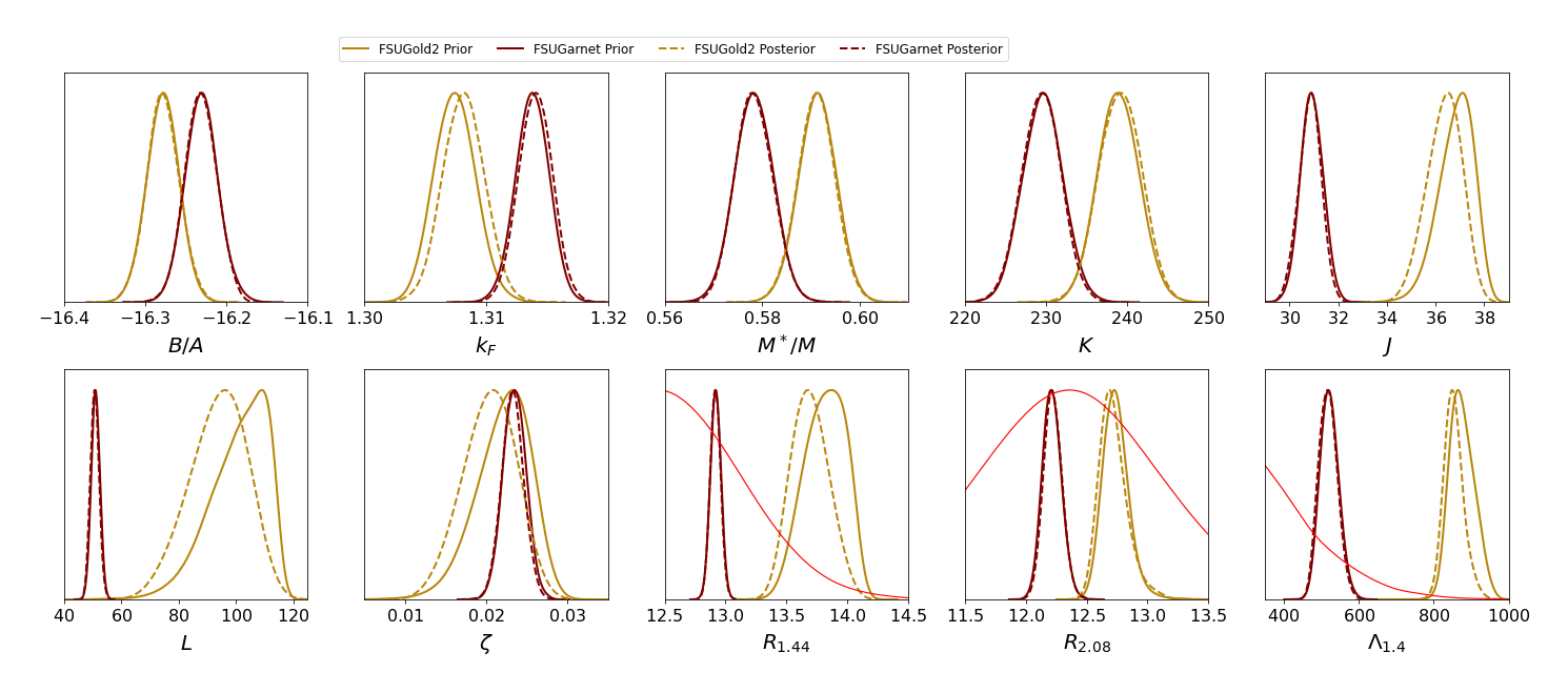
Figure 1: MCMC results obtained by sampling the posterior distribution of parameters using only astrophysical data. The two covariant EDFs, FSUGold2 and FSUGarnet, are displayed with their respective colors. The solid red line depicts the probability distribution for the three astrophysical observables quoted in Eq.(19). The binding energy per nucleon $B/A$, the incompressibility coefficient $K$, the symmetry energy $J$, and the slope of the symmetry energy $L$—all evaluated at saturation density—are given in MeV. The Fermi momentum at saturation $k_{\rm F}$ is given in units of fm^-1, stellar radii are reported in km, while the effective mass at saturation $M^{\ast}/M$, $\zeta$, and the tidal deformability $\Lambda_{1.4}$ are all dimensionless quantities.

In contrast, the Bayesian refinement has a visible impact on various isovector quantities predicted by FSUGold2, such as $J$, $L$, $R_{1.44}$ and $\Lambda_{1.4}$. As opposed to FSUGarnet, FSUGold2 favors a fairly stiff symmetry energy. The astrophysical data seems to disfavor such a stiff symmetry energy and induces a mild softening. Such a softening of the symmetry energy must be compensated in order to be able to account for the existence of two-solar-mass neutron stars. Hence, the softening of the symmetry energy must be accompanied by a reduction of the coupling constant $\zeta$ that stiffens the EOS of symmetric nuclear matter in the high density region; see Fig.1. Although some changes are clearly evident in Fig.1—especially in the case of FSUGold2—we conclude that for this particular set of covariant EDFs, astrophysical observations alone do not generate dramatic changes to the EOS, even after adopting the fairly optimistic errors in the neutron star radii quoted in Ref. Miller et al. (2021).

III.2 Adding $\chi$EFT Information

Whereas astrophysical data informs the EOS in the vicinity of two times saturation density, $\chi$EFT provides important constraints at and below saturation density. For a model that predicts a fairly soft EOS such as FSUGarnet, we expect a modest impact from $\chi$EFT. In contrast, we anticipate that the much stiffer FSUGold2 functional will be strongly affected by this new information.

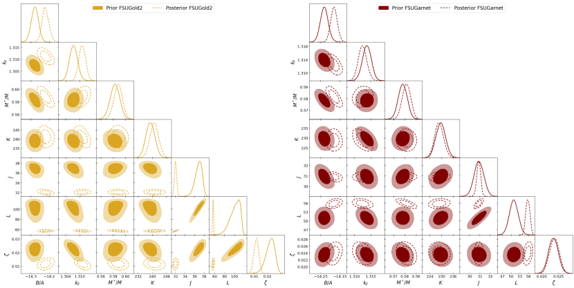
Figure 2: Corner plot for both the prior and posterior distribution of bulk matter properties obtained after implementing the Metropolis-Hasting algorithm. The posterior distributions (dashed lines) incorporate both astrophysical and $\chi$EFT constraints into the likelihood function. A total of 10 thousand MCMC steps were used to sample the posterior distribution and 50 thousand for the prior distribution. The ellipses represent 68% and 95% confidence intervals and we have adopted the same units and color convention as in Fig.1.

We display in Fig.2 corner plots for both FSUGold2 and FSUGarnet obtained after implementing the Metropolis-Hasting algorithm. Unlike Fig.1, the posterior distribution of bulk parameters is informed by a likelihood function that now contains both astrophysical and $\chi$EFT constraints. The covariance ellipses displayed in the figure represent 68% and 95% confidence intervals. The first thing to notice is that $\chi$EFT shifts slightly the saturation point, an effect that is absent from Fig. 1 when only astrophysical information was used. Given that $\chi$EFT predicts a saturation point that is in conflict with the predictions from DFT, such a shift may have been expected. Relative to DFT predictions—which incorporate nuclear information into the calibration of the functional—$\chi$EFT tends to either saturate at higher density or to underbind the system Drischler et al. (2021). However, as anticipated, the most dramatic changes involve the two symmetry energy parameters $J$ and $L$, especially for FSUGold2. Interestingly, in the case of FSUGarnet, $\chi$EFT actually favors a slight stiffening of the symmetry energy. Also noticeable is the significant reduction in the theoretical uncertainty in both $J$ and $L$, suggesting that the symmetry energy is much better constrained in $\chi$EFT than in DFT, where the calibration of the EDFs is hindered by the lack of isovector observables. This fact underscores the important role that high-order $\chi$EFT calculations play in the calibration of energy density functionals. We note that beyond the dramatic softening of the symmetry energy experienced by FSUGold2, a strong correlation also develops between $L$ and the isoscalar parameter $\zeta$. As already indicated, the quartic coupling $\zeta$ controls the high density component of the EOS, so if $L$ goes down, then $\zeta$ must compensate for such a change in order to be able to support $2{\rm M}_{\odot}$ neutron stars against gravitational collapse.

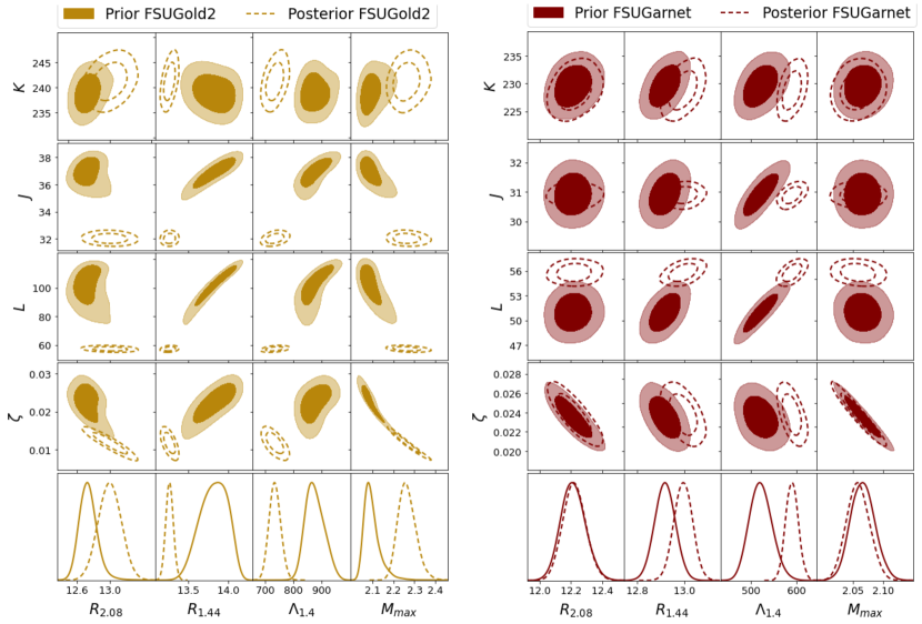
Figure 3: Correlations between astrophysical observables and bulk properties after implementing the Metropolis-Hasting algorithm. The posterior distributions (dashed lines) incorporate both astrophysical and $\chi$EFT constraints into the likelihood function. A total of 10 thousand MCMC steps were used to sample the posterior distribution and 50 thousand for the prior distribution. The ellipses represent 68% and 95% confidence intervals and we have adopted the same units and color convention as in Fig.1.

Having examined the statistical correlations between the various bulk parameters in Fig.2, we now proceed to assess in Fig.3 the impact of the Bayesian refinement on the astrophysical observables that were used to inform the likelihood function. As before, the impact of the refinement on FSUGarnet is a modest stiffening driven by $\chi$EFT that results in a slight increase to both the radius and tidal deformability of a $1.4{\rm M}_{\odot}$ neutron star. In the case of FSUGold2, it is interesting to note that the softening generated by $\chi$EFT reduces significantly the radius and tidal deformability of a $1.4{\rm M}_{\odot}$, but increases the maximum stellar mass and the radius of a $2{\rm M}_{\odot}$ neutron star. Again, this behavior is associated with the stiffening of the EOS at high densities required to compensate for the softening of the symmetry energy. Moreover, it also indicates—as expected—that the behavior of the symmetry energy at saturation density correlates poorly with the behavior of massive stars that is dominated by the EOS at densities that cannot be probed in terrestrial laboratories.

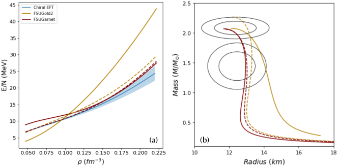
Figure 4: (a) Equation of state for pure neutron matter as predicted by FSUGold2 Chen and Piekarewicz (2014), FSUGarnet Chen and Piekarewicz (2015), and a $\chi$EFT calculation correct up to next-to-next-to-next-leading order (N³LO) in the chiral expansion Drischler et al. (2021). Predictions from FSUGold2 and FSUGarnet are displayed with their respective colors, with the solid and dashed lines representing results before and after the Bayesian refinement, respectively. (b) Mass-Radius relationship as predicted by FSUGold2 and FSUGarnet, both pre and post refinement The covariance ellipses represent the 68% and 95% confidence intervals following Eq.(19).

The impact of the refinement on the two covariant EDFs used in this work is summarized in Fig.4. Shown on the left-hand panel using the same color convention as in Fig.1 are FSUGold2 and FSUGarnet predictions for the equation of state of pure neutron matter; for ease of viewing, only central values are shown. In turn, the blue bands display $\chi$EFT predictions correct up to next-to-next-to-next-leading order Drischler et al. (2021). As inferred from our previous discussion, the impact on FSUGarnet is modest, except at the lowest densities. The situation, however, is radically different in the case of FSUGold2. As we show below in Sec.III.4, the dramatic softening of the EOS will have important consequences on the prediction of the neutron skin thickness of ²⁰⁸Pb. Interestingly, as shown on the right-hand panel in Fig.4, the softening induced at intermediate densities also generates a stiffening of FSUGold2 at the highest densities, resulting in a maximum neutron star mass of about $2.3{\rm M}_{\odot}$. Lastly, the covariance ellipses display in the figure represent the 68% and 95% confidence intervals for the two NICER measurements Miller et al. (2021). After refinement, the predictions of both FSUGold2 and FSUGarnet fall comfortably within the 68% confidence ellipses.

The observation of neutron stars with masses in the vicinity of two solar masses requires a stiff EOS in order to support them against gravitational collapse Demorest et al. (2010); Antoniadis et al. (2013); Cromartie et al. (2019); Fonseca et al. (2021). Having incorporated both theoretical and observational information into the model refinement, we now assess its impact on the EOS of neutron star matter $P\!=\!P({{\varepsilon}})$—and on the associated speed of sound defined as the derivative of the pressure with respect to the energy density:

$$\frac{c_{s}^{2}}{c^{2}}=\frac{dP({{\varepsilon}})}{d{{\varepsilon}}}.$$ (25)

Interest in the speed of sound in neutron stars was inspired by a conjecture grounded in holography that suggests that the conformal limit of $c_{s}^{2}/c^{2}\!=\!1/3$ represents an upper bound for a broad class of four-dimensional theories Cherman et al. (2009). In the context of neutron stars, Bedaque and Steiner suggested that the existence of heavy neutron stars is in strong tension with the conformal limit Bedaque and Steiner (2015). Later on, studies that incorporated the tidal polarizability as an additional constraint on the EOS—both before Moustakidis et al. (2017) and after Reed and Horowitz (2020) GW170817 Abbott et al. (2017)—also seem to suggest that the existence of heavy neutron stars is likely responsible for violating the conformal limit. Further, within the $\chi$EFT framework, it was found that the conformal limit is in tension with current nuclear physics constraints and observations of two-solar-mass neutron stars Tews et al. (2018). The paper concludes with the fairly provocative statement that if the conformal limit holds at all densities, then nuclear physics models break down below twice saturation density.

To confront these assertions, we display in Fig.5 predictions from both FSUGold2 and FSUGarnet before and after refinement. The EOS displays the various regions of the neutron star, particularly the outer crust, the inner crust, and the uniform liquid core. Concerning the speed of sound displayed on the inset in the figure, the conformal limit is already violated around two and a half times nuclear saturation density. Also shown on the inset is the maximum density reached at the center of the maximum mass configuration, a density that is significantly smaller than $\rho_{{}_{\!\rm pQCD}}\!\sim\!40\,\rho_{0}$, namely, the density at which QCD becomes perturbative and the conformal limit may be recovered. For a recent discussion on the role that perturbative QCD may play in constraining the EOS at neutron-star densities see Ref. Komoltsev and Kurkela (2022) and references contained therein.

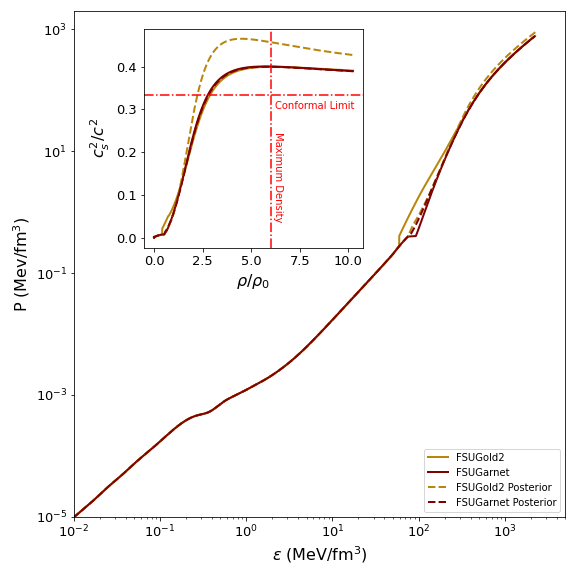
Figure 5: Equation of state of neutron star matter and the associated speed of sound as predicted by FSUGold2 and FSUGarnet, with the solid and dashed lines representing results before and after the Bayesian refinement, respectively. The red dot-dashed lines on the inset indicate the conformal limit and the maximum density reached at the core at the maximum mass configuration.

We also observe on the inset of Fig.5 that the the predictions of FSUGold2 after refinement suggest that the conformal limit is violated even earlier, at about twice $\rho_{0}$. This region of density is particularly interesting as it may be studied in the laboratory using energetic nuclear reactions that may compress and probe nuclear matter in the vicinity of twice nuclear saturation density. Indeed, this is one of the main science drivers behind the proposed FRIB-400 upgrade of the Facility for Rare Isotope Beams (FRIB). Such a rapid increase in the speed of sound displayed by the posterior distribution of FSUGold2 is driven by its prediction of a maximum neutron star mass of $2.3{\rm M}_{\odot}$; see Fig.4. Particularly relevant to this fact is the recent report of the “black-widow” system PSR J0952-0607 with an extremely large pulsar mass of $(2.35\!\pm\!0.17){\rm M}_{\odot}$ Romani et al. (2022). If the existence of such massive neutron stars can be confirmed with better statistics, then—and not withstanding the small tidal deformability reported by the LIGO-Virgo collaboration Abbott et al. (2018)—the violation of the conformal limit in neutron star interiors seems unavoidable.

Before leaving this section we list in Table 2 the optimal parameter set for both FSUGold2 and FSUGarnet after refinement. We underscore, however, that these are optimal (or central) values, as the EDFs after refinement are properly described by a statistical distribution of model parameters. Using this optimal set of parameters, we list in Table 3 central values for the resulting bulk parameters after the Bayesian refinement. Most notably is the softening of the symmetry energy of FSUGold2, largely induced by the inclusion of $\chi$EFT information; see Table 1 for comparison.

​Model	$m_{\rm s}$	$m_{\rm v}$	$m_{\rho}$	$g_{\rm s}^{2}$	$g_{\rm v}^{2}$	$g_{\rho}^{2}$	$\kappa$	$\lambda$	$\zeta$	$\Lambda_{\rm v}$
FSUGold2+R	501.611	782.500	763.000	103.760	169.410	128.301	3.79239	$-$0.010635	0.011660	0.0316212
FSUGarnet+R	495.633	782.500	763.000	109.130	186.481	142.966	3.25933	$-$0.003285	0.023812	0.038274

Table 2: Central values for the model parameters FSUGold2 and FSUGarnet after Bayesian refinement. The parameter $\kappa$ and the meson masses $m_{\rm s}$, $m_{\rm v}$, and $m_{\rho}$ are all given in MeV, and the nucleon mass has been fixed at $M\!=\!939$ MeV.

​Model	$\rho_{0}(\text{fm}^{-3})$	${{\epsilon}}_{0}$ (MeV)	$M^{\star}/M$	K (MeV)	J (MeV)	L (MeV)	$\zeta$
FSUGold2+R	0.1522	-16.22	0.594	241.22	32.03	57.20	0.0117
FSUGarnet+R	0.1527	-16.18	0.582	228.77	30.89	55.79	0.0238

Table 3: Central values for various bulk properties of infinite nuclear matter as predicted by FSUGold2 and FSUGarnet after the Bayesian refinement; compare to Table 1.

III.3 Heaven and Earth

One of the most captivating features of neutron stars is the powerful connection between laboratory experiments and astronomical observations. For example, it is well known that the slope of the symmetry energy $L$, which can be determined by measuring the neutron skin thickness of heavy nuclei, controls the radius of low-mass neutron stars Horowitz and Piekarewicz (2001a, b); Carriere et al. (2003); Lattimer and Prakash (2007). One expects, however, that the correlation between the thickness of the neutron skin and the neutron star radius will weaken as the stellar mass increases. It is the aim of this section to identify the density region that has the strongest impact on the development of the stellar radius.

To do so we implement the following procedure. First, as part of the Bayesian refinement, we generate multiple samples of various observables distributed according to the posterior distribution. Second, for each of the samples, we isolate the entire mass-radius relationship and the associated equation of state. We then proceed to store the pressure $P_{\!\rho}$ at various values of the baryon density $\rho$ as well as the predicted stellar radii $R_{M}$ over a given mass ($M$) range. Finally, once all Monte Carlo samples have been generated, we compute the Pearson correlation coefficient between $R_{M}$ and $P_{\!\rho}$.

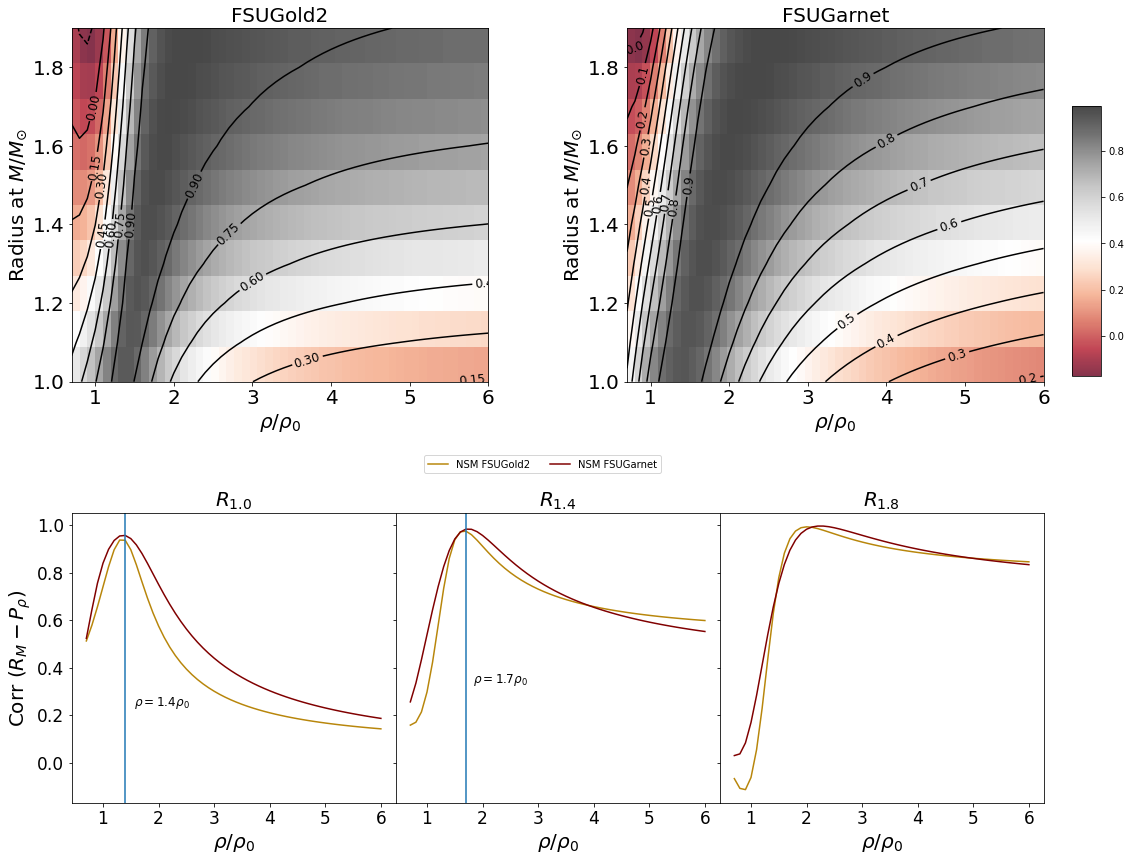
Figure 6: Pearson correlation coefficients inferred from the posterior distribution of FSUGold2 and FSUGarnet. The top panel displays contour plots labeled by the correlation coefficient between the stellar radius of a given mass configuration $R_{M}$ and the associated pressure support as a function of density $P_{\!\rho}$. The bottom panel displays the $R_{M}\!-\!P_{\!\rho}$ correlation coefficient for three neutron stars with individual masses of 1.0, 1.4, and 1.8 ${\rm M}_{\odot}$.

Shown on the top panel of Fig. 6 is a heat map that displays the $R_{M}\!-\!P_{\!\rho}$ correlation predicted from the FSUGold2 and FSUGarnet posterior distribution, with the various contour lines labeled according to the value of the correlation coefficient. For example, in the case of FSUGold2, the pressure in the narrow $(1.2\!-\!1.5)\,\rho_{0}$ density region correlates with the radius of a $1\,{\rm M}_{\odot}$ neutron star to better than 90%. This behavior is better appreciated in the lower panel of Fig. 6, which clearly indicates that the radius of a $1\,{\rm M}_{\odot}$ neutron star is dominated by the pressure over a very narrow range of densities. This validates the claim that laboratory experiments that determine the neutron skin thickness of heavy nuclei place stringent constraints on the radius of low-mass neutron stars Carriere et al. (2003). For a “canonical” $1.4\,{\rm M}_{\odot}$ neutron star, the strongest correlation develops at $1.7\,\rho_{0}$, yet larger values of the density that are no longer accessible in the laboratory continue to make an important contribution. Finally, for a $1.8\,{\rm M}_{\odot}$ neutron star, the relevant region of densities is too high and wide for laboratory experiments to play a pivotal role in the determination of the stellar radius.

III.4 Neutron Skins

In the previous sections we have demonstrated how the Bayesian refinement of two previously calibrated covariant EDFs provides updated predictions that are in agreement with a large set of observables ranging from the properties of finite nuclei to the structure of neutron stars. Perhaps the only exception noticed so far is the tidal deformability of a $1.4\,{\rm M}_{\odot}$ neutron star predicted by FSUGold2. Even after the significant softening of the symmetry energy, FSUGold2 still predicts a tidal deformability of $\Lambda_{1.4}\!\approx\!740\pm 40$ that lies significantly outside the 90% confidence interval of $\Lambda_{1.4}\!=\!190^{+390}_{-120}$ quoted by the LIGO-Virgo collaboration Abbott et al. (2018). We note, however, that such a small tidal deformability is not without question. Indeed, a recent analysis that excluded waveform information beyond a certain frequency suggests significant larger values for the tidal deformability; see in particular Fig.8 of Ref. Gamba et al. (2021). Under such a scenario, the refined FSUGold2 prediction for $\Lambda_{1.4}$ is no longer excluded.

There is, however, a laboratory observable that seems to disfavor the softening induced on FSUGold2: the neutron skin thickness of ²⁰⁸Pb. Given the strong correlation between $L$ and the neutron skin thickness of ²⁰⁸Pb Brown (2000); Furnstahl (2002); Centelles et al. (2009); Roca-Maza et al. (2011), we expect that the significant lower value of $L$ obtained after refinement will be in conflict with the PREX measurement Adhikari et al. (2021), which instead favors a fairly stiff symmetry energy Reed et al. (2021). Indeed, an interesting tension has emerged when confronting the PREX Adhikari et al. (2021) and CREX Adhikari et al. (2022) measurements. Whereas the extracted neutron skin in ²⁰⁸Pb is thick, CREX reported a very thin neutron skin in ⁴⁸Ca; see Table 4. This presents a problem for the class of covariant EDFs used in this work, because the correlation between the neutron skins of ²⁰⁸Pb and ⁴⁸Ca is predicted to be strong Piekarewicz (2021); Giuliani et al. (2023).

Besides the neutron skin thickness of ²⁰⁸Pb and ⁴⁸Ca, we list in Table 4 results for the charge and weak-charge radii, where the contribution from the finite nucleon size has been included Horowitz and Piekarewicz (2012). If the elastic form factor has been measured over a very wide range of momentum transfers, then the experimental radius may be extracted directly from the slope at the origin. This is the case for the charge radius of both ⁴⁸Ca and ²⁰⁸Pb Angeli and Marinova (2013). Instead, given that PREX and CREX measured the weak form factor at only one momentum transfer, the extraction of the two weak-charge radii acquires a mild model dependence.

We observe in Table 4 that the agreement between the FSUGold2 predictions and the PREX results are in excellent agreement, suggesting that the symmetry energy is indeed stiff Reed et al. (2021). However, once the Bayesian refinement is implemented (FSUGold2+R) the excellent agreement is lost: the neutron skin thickness of ²⁰⁸Pb goes down from the experimentally consistent value o f $R_{\rm skin}^{208}\!=\!0.285\,{\rm fm}$ all the way down to $R_{\rm skin}^{208}\!=\!0.203\,{\rm fm}$. In the case of ⁴⁸Ca, the softening of the symmetry energy post-refinement moves the theoretical prediction in the direction of the experiment, but not nearly as much as it is required. That is, the neutron skin thickness of ⁴⁸Ca, goes down from $R_{\rm skin}^{48}\!=\!0.231\,{\rm fm}$ to $R_{\rm skin}^{48}\!=\!0.197\,{\rm fm}$, which remains far from the quoted CREX value of $R_{\rm skin}^{48}\!=\!0.121(35)\,{\rm fm}$ Adhikari et al. (2022). It is important to note that after refinement the theoretical uncertainty in both $R_{\rm skin}^{208}$ and $R_{\rm skin}^{48}$ is significantly reduced.

To further appreciate the present predicament, we display in Fig.7—alongside FSUGold2 and FSUGold2+R—predictions for the neutron skin thickness of ⁴⁸Ca and ²⁰⁸Pb using the same set of covariant EDFs employed in Ref. Reed et al. (2021) to analyze the PREX results. This set includes the original (before refinement) FSUGarnet predictions. Also shown are the 67% and 90% confidence ellipses together with the central values and 1$\sigma$ errors quoted by the PREX/CREX collaboration Adhikari et al. (2022). The nearly perfect linear correlation between $R_{\rm skin}^{208}$ and $R_{\rm skin}^{48}$ is evident in the figure, yet none of the predictions reside inside the 90% confidence ellipse. As indicated earlier, the original FSUGold2 prediction reproduces the PREX result, but grossly overestimates the CREX value. The Bayesian refinement does not improve the situation, as the new prediction simply slides along the regression line.

​​Model (208Pb)	$R_{\rm ch}$	$R_{\rm wk}$	$R_{\rm ch}\!-\!R_{\rm wk}$	$R_{n}\!-\!R_{p}$
​​FSUGold2	5.491(6)	5.801(19)	0.310(16)	0.285(15)
FSUGold2+R	5.517(4)	5.743(05)	0.226(03)	0.203(03)
Experiment	5.501(1)	5.800(75)	0.299(75)	0.283(71)
​​Model (48Ca)	$R_{\rm ch}$	$R_{\rm wk}$	$R_{\rm ch}\!-\!R_{\rm wk}$	$R_{n}\!-\!R_{p}$
​​FSUGold2	3.426(3)	3.707(07)	0.281(08)	0.231(08)
FSUGold2+R	3.477(8)	3.722(09)	0.245(02)	0.197(02)
Experiment	3.477(2)	3.636(35)	0.159(35)	0.121(35)

Table 4: Predictions for FSUGold2 before and after refinement (+R) for the charge radius, weak radius, weak skin and neutron skin (all in fm) of ²⁰⁸Pb and ⁴⁸Ca, as compared with the experimental values extracted from PREX Adhikari et al. (2021) and CREX Adhikari et al. (2022).

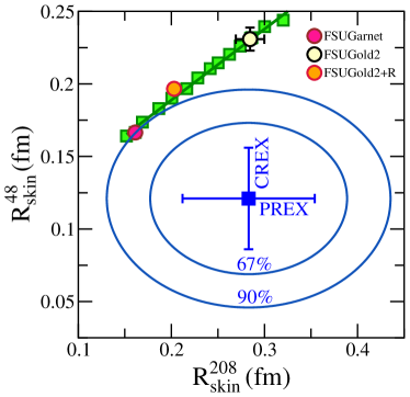
Figure 7: Predictions for the neutron skin thickness of ²⁰⁸Pb and ⁴⁸Ca from the same set of covariant EDFs used in Ref.Reed et al. (2021), including the original FSUGarnet model. Also shown are predictions before and after refinement from FSUGold2 and FSUGold2+R, respectively. Central values and 1$\sigma$ errors together with 67% and 90% confidence ellipses are obtained from Ref. Adhikari et al. (2022).

Perhaps the obvious deficiency displayed in Fig.7 may be an indication that the physics encoded in the Lagrangian density given in Eq.(1) is incomplete. After all, with only two isovector parameters ($g_{\rho}$ and $\Lambda_{\rm v}$) it may be difficult to break the strong correlation between the neutron skins of ⁴⁸Ca and ²⁰⁸Pb. We are currently working on extending the isovector sector of the covariant EDFs. Although models with a stronger theoretical underpinning may be able to reconcile both measurements at some level Hu et al. (2022), it is increasingly apparent that the skin-skin correlation can not be entirely broken. As such, one must conclude that—at present—no single theoretical framework can reproduce simultaneously the PREX and CREX results Reinhard et al. (2022); Mondal and Gulminelli (2023); Yüksel and Paar (2023); Zhang and Chen (2022); Papakonstantinou (2022).

Another possible resolution of the present dilemma is to appeal to the rather large experimental error bars. In this context, the only option is a more precise determination of $R_{\rm skin}^{208}$ at the future Mainz Energy-recovery Superconducting Accelerator (MESA) Becker et al. (2018). Although a factor-of-two improvement in $R_{\rm skin}^{208}$ is realistic, the reality is that such an experiment is unlikely to be commissioned before the end of this decade. Regardless, we advocate for a more interesting resolution to the dilemma, namely, that the answer is not hiding behind the experimental error bars but rather, that the answer may require to uncover some missing physics absent from existing theoretical descriptions.

IV Conclusions

Progress in our understanding of the equation of state of neutron star matter has grown significantly during the last few years. The aim of this paper was to incorporate the latest information on neutron star properties to improve existing covariant energy density functionals that were largely calibrated by the properties of finite nuclei. Among the new properties informing the refinement of the functionals are: maximum stellar masses reported from pulsar timing measurements Cromartie et al. (2019); Fonseca et al. (2021), the simultaneous extraction of stellar radii and masses of two sources by the NICER mission Riley et al. (2019); Miller et al. (2019, 2021); Riley et al. (2021), tidal information from the LIGO-Virgo collaboration Abbott et al. (2017, 2018), and predictions for the EOS of pure neutron matter from chiral effective field theory Drischler et al. (2021). This new information was incorporated in a likelihood function which, through Bayesian inference, was used to refine two existing density functionals whose covariance matrices served as prior distributions of model parameters.

The two existing covariant EDFs, FSUGold2 Chen and Piekarewicz (2014) and FSUGarnet Chen and Piekarewicz (2015), followed a very similar fitting protocol to calibrated the model parameters. Given that the spherical nuclei used in the calibration are either stable or long-lived, both models predict similar isoscalar observables, such as the bulk properties of symmetric nuclear matter listed in Table 1. In contrast, at the time of the calibration, the database of strong isovector observables was very sparse, leading to a poorly constrained density dependence of the symmetry energy. Hence, the two EDFs adopted in this work were calibrated by selecting symmetry energies with a density dependence at the opposite ends of the spectrum, with FSUGold2 being stiff and FSUGarnet being soft. Motivated by the recent proliferation of strong isovector indicators, we implemented a Bayesian refinement of the model parameters by sampling posterior distributions via a Metropolis-Hastings algorithm.

The refinement was implemented in two stages. We started by assessing solely the impact of astrophysical observables and later added $\chi$EFT predictions. When only astrophysical information was included, changes to the predictions of both models were modest, especially in the case FSUGarnet. For FSUGold2, the refinement slightly softens the symmetry energy resulting in mild reductions in both the slope of the symmetry energy $L$ and the radius of a $1.44\,{\rm M}_{\odot}$ neutron star. However, the situation changed dramatically once $\chi$-EFT predictions were incorporated. This we attribute to the sharp $\chi$EFT predictions relative to the fairly large astrophysical uncertainties. Although $\chi$EFT predicts a rather soft EOS for pure neutron matter, $\chi$EFT information stiffens the even softer symmetry energy predicted by FSUGarnet. However, the impact on FSUGold2 is dramatic: the symmetry energy at saturation density $J$, its slope $L$, and the non-linear coupling $\zeta$ were all greatly sharpened and reduced; see Fig.2. Note that the reduction in the value of the non-linear coupling $\zeta$, which implies a stiffening of the EOS of symmetric nuclear matter, is required to compensate for the softening of the symmetry energy. Without such a stiffening, the resulting EOS would not be able to support massive neutron stars. Indeed, after refinement, FSUGold2 predicts a maximum neutron star mass of about $2.3\,{\rm M}_{\odot}$, consistent with the black-widow pulsar with a mass of $(2.35\!\pm\!0.17){\rm M}_{\odot}$ Romani et al. (2022). As expected, the induced softening of the symmetry energy reduces the stellar radius and tidal deformability of a $1.4\,{\rm M}_{\odot}$ neutron star. However, the reduction in $\Lambda_{1.4}$ is not sufficient to reproduce the fairly small value quoted by the LIGO-Virgo collaboration Abbott et al. (2018), although larger values do not seem to be completely ruled out Gamba et al. (2021).

Once both models were refined, we reported predictions for the mass-radius relation, the underlying EOS, and the associated speed of sound. Both of the predicted mass-radius relations are fully consistent with the reported NICER values for both PSR J0740+6620 and PSR J0030+0451. In particular, the existence of two-solar-mass neutron stars demands that the EOS be stiff at the highest densities encountered in the stellar core, which for the models under consideration reaches a value in the vicinity of $6\rho_{0}$. Notably, demands for a stiff EOS resulted in a violation of the conformal limit on the speed of sound at the relatively low densities of about $(2\!-\!2.5)\,\rho_{0}$, a range of densities that could be probed in the laboratory if the proposed FRIB-400 upgrade becomes a reality.

Whereas the Bayesian refinement of existing EDFs reproduce a large body of experimental and observational data over a broad range of densities, the induced softening of the symmetry energy is in conflict with recent results by the PREX and CREX collaborations on the neutron skin thickness of ²⁰⁸Pb Adhikari et al. (2021) and ⁴⁸Ca Adhikari et al. (2022), respectively. Although the experimental error bars are large, none of our models are able to reconcile the very thick neutron skin in ²⁰⁸Pb with the very thin neutron skin in ⁴⁸Ca. From the perspective of covariant EDFs, the problem is especially challenging given that the neutron skin thickness of ²⁰⁸Pb and ⁴⁸Ca are strongly correlated Piekarewicz (2021). Plans are currently under way to enlarge the isovector sector of the covariant EDFs in the hope of breaking such a correlation. However, the challenge to reconcile both measurements appears to go beyond the class of covariant EDFs considered in this work Reinhard et al. (2022); Mondal and Gulminelli (2023); Yüksel and Paar (2023); Zhang and Chen (2022); Papakonstantinou (2022). Only time will tell whether the resolution of this puzzle is hiding behind the large experimental error bars or whether it demands a more ingenious solution.

- (1) G. Baym, Proceedings of the 8th International Conference on Quarks and Nuclear Physics (QNP2018), 10.7566/JPSCP.26.011001.
- Baym et al. (2018) G. Baym, T. Hatsuda, T. Kojo, P. D. Powell, Y. Song, and T. Takatsuka, Rept. Prog. Phys. 81, 056902 (2018).
- Hebeler and Schwenk (2010) K. Hebeler and A. Schwenk, Phys. Rev. C82, 014314 (2010).
- Tews et al. (2013) I. Tews, T. Kruger, K. Hebeler, and A. Schwenk, Phys. Rev. Lett. 110, 032504 (2013).
- Kruger et al. (2013) T. Kruger, I. Tews, K. Hebeler, and A. Schwenk, Phys. Rev. C88, 025802 (2013).
- Lonardoni et al. (2020) D. Lonardoni, I. Tews, S. Gandolfi, and J. Carlson, Phys. Rev. Res. 2, 022033 (2020).
- Drischler et al. (2021) C. Drischler, J. W. Holt, and C. Wellenhofer, Ann. Rev. Nucl. Part. Sci. 71, 403 (2021).
- Sammarruca and Millerson (2021) F. Sammarruca and R. Millerson, Phys. Rev. C 104, 034308 (2021).
- Sammarruca and Millerson (2022) F. Sammarruca and R. Millerson, Universe 8, 133 (2022).
- Abrahamyan et al. (2012) S. Abrahamyan, Z. Ahmed, H. Albataineh, K. Aniol, D. S. Armstrong, et al., Phys. Rev. Lett. 108, 112502 (2012).
- Horowitz et al. (2012) C. J. Horowitz, Z. Ahmed, C. M. Jen, A. Rakhman, P. A. Souder, et al., Phys. Rev. C85, 032501 (2012).
- Adhikari et al. (2021) D. Adhikari et al. (PREX), Phys. Rev. Lett. 126, 172502 (2021).
- Reed et al. (2021) B. T. Reed, F. J. Fattoyev, C. J. Horowitz, and J. Piekarewicz, Phys. Rev. Lett. 126, 172503 (2021).
- Piekarewicz (2022) J. Piekarewicz, (2022), arXiv:2209.14877 [nucl-th] .
- Abbott et al. (2017) B. P. Abbott et al. (Virgo, LIGO Scientific), Phys. Rev. Lett. 119, 161101 (2017).
- Abbott et al. (2018) B. P. Abbott et al. (Virgo, LIGO Scientific), Phys. Rev. Lett. 121, 161101 (2018).
- Riley et al. (2019) T. E. Riley et al., Astrophys. J. Lett. 887, L21 (2019).
- Miller et al. (2019) M. C. Miller et al., Astrophys. J. Lett. 887, L24 (2019).
- Miller et al. (2021) M. C. Miller et al., Astrophys. J. Lett. 918, L28 (2021).
- Riley et al. (2021) T. E. Riley et al., Astrophys. J. Lett. 918, L27 (2021).
- Demorest et al. (2010) P. Demorest, T. Pennucci, S. Ransom, M. Roberts, and J. Hessels, Nature 467, 1081 (2010).
- Antoniadis et al. (2013) J. Antoniadis, P. C. Freire, N. Wex, T. M. Tauris, R. S. Lynch, et al., Science 340, 6131 (2013).
- Cromartie et al. (2019) H. T. Cromartie et al., Nat. Astron. 4, 72 (2019).
- Fonseca et al. (2021) E. Fonseca et al., Astrophys. J. Lett. 915, L12 (2021).
- Adhikari et al. (2022) D. Adhikari et al. (CREX), Phys. Rev. Lett. 129, 042501 (2022).
- Gamba et al. (2021) R. Gamba, M. Breschi, S. Bernuzzi, M. Agathos, and A. Nagar, Phys. Rev. D 103, 124015 (2021).
- Radice and Dai (2019) D. Radice and L. Dai, Eur. Phys. J. A 55, 50 (2019).
- Alford et al. (2022) M. G. Alford, L. Brodie, A. Haber, and I. Tews, Phys. Rev. C 106, 055804 (2022).
- Chen and Piekarewicz (2014) W.-C. Chen and J. Piekarewicz, Phys. Rev. C90, 044305 (2014).
- Chen and Piekarewicz (2015) W.-C. Chen and J. Piekarewicz, Phys. Lett. B748, 284 (2015).
- Walecka (1974) J. D. Walecka, Annals Phys. 83, 491 (1974).
- Boguta and Bodmer (1977) J. Boguta and A. R. Bodmer, Nucl. Phys. A292, 413 (1977).
- Serot and Walecka (1986) B. D. Serot and J. D. Walecka, Adv. Nucl. Phys. 16, 1 (1986).
- Mueller and Serot (1996) H. Mueller and B. D. Serot, Nucl. Phys. A606, 508 (1996).
- Serot and Walecka (1997) B. D. Serot and J. D. Walecka, Int. J. Mod. Phys. E6, 515 (1997).
- Horowitz and Piekarewicz (2001a) C. J. Horowitz and J. Piekarewicz, Phys. Rev. Lett. 86, 5647 (2001a).
- Satpathy and Nayak (1983) L. Satpathy and R. Nayak, Phys. Rev. Lett. 51, 1243 (1983).
- Baym et al. (1971) G. Baym, C. Pethick, and P. Sutherland, Astrophys. J. 170, 299 (1971).
- Roca-Maza and Piekarewicz (2008) X. Roca-Maza and J. Piekarewicz, Phys. Rev. C78, 025807 (2008).
- Feynman et al. (1949) R. Feynman, N. Metropolis, and E. Teller, Phys. Rev. 75, 1561 (1949).
- Haensel et al. (1989) P. Haensel, J. L. Zdunik, and J. Dobaczewski, Astron. Astrophys. 222, 353 (1989).
- Piekarewicz (2014) J. Piekarewicz, AIP Conf. Proc. 1595, 76 (2014).
- Ravenhall et al. (1983) D. G. Ravenhall, C. J. Pethick, and J. R. Wilson, Phys. Rev. Lett. 50, 2066 (1983).
- Hashimoto et al. (1984) M. Hashimoto, H. Seki, and M. Yamada, Prog. Theor. Phys. 71, 320 (1984).
- Lorenz et al. (1993) C. P. Lorenz, D. G. Ravenhall, and C. J. Pethick, Phys. Rev. Lett. 70, 379 (1993).
- Fattoyev et al. (2018) F. Fattoyev, E. F. Brown, A. Cumming, A. Deibel, C. Horowitz, B.-A. Li, and Z. Lin, Phys. Rev. C 98, 025801 (2018).
- Negele and Vautherin (1973) J. W. Negele and D. Vautherin, Nucl. Phys. A207, 298 (1973).
- Carriere et al. (2003) J. Carriere, C. J. Horowitz, and J. Piekarewicz, Astrophys. J. 593, 463 (2003).
- Kubis (2007) S. Kubis, Phys. Rev. C 76, 025801 (2007).
- Routray et al. (2016) T. R. Routray, X. Viñas, D. N. Basu, S. P. Pattnaik, M. Centelles, L. Robledo, and B. Behera, J. Phys. G 43, 105101 (2016).
- Piekarewicz and Centelles (2009) J. Piekarewicz and M. Centelles, Phys. Rev. C79, 054311 (2009).
- PRA-Editors (2011) PRA-Editors, Phys. Rev. A 83, 040001 (2011).
- Gregory (2005) P. C. Gregory, “Bayesian logical data analysis for the physical sciences,” (Cambridge University Press, Cambridge, UK, 2005).
- Stone (2013) J. V. Stone, “Bayes’ rule: A tutorial introduction to bayesian analysis,” (Sebtel Press, Sheffield, UK, 2013).
- Fröhner (1996) F. H. Fröhner, in Maximum Entropy and Bayesian Methods, edited by K. M. Hanson and R. N. Silver (Springer Netherlands, Dordrecht, 1996) pp. 393–406.
- Steiner (2018) A. W. Steiner, (2018), arXiv:1802.05339 [physics.data-an] .
- Brandes et al. (2023) L. Brandes, W. Weise, and N. Kaiser, Phys. Rev. D 107, 014011 (2023).
- Cherman et al. (2009) A. Cherman, T. D. Cohen, and A. Nellore, Phys. Rev. D 80, 066003 (2009).
- Bedaque and Steiner (2015) P. Bedaque and A. W. Steiner, Phys. Rev. Lett. 114, 031103 (2015).
- Moustakidis et al. (2017) C. C. Moustakidis, T. Gaitanos, C. Margaritis, and G. A. Lalazissis, Phys. Rev. C 95, 045801 (2017), [Erratum: Phys.Rev.C 95, 059904 (2017)].
- Reed and Horowitz (2020) B. Reed and C. J. Horowitz, Phys. Rev. C 101, 045803 (2020).
- Tews et al. (2018) I. Tews, J. Carlson, S. Gandolfi, and S. Reddy, Astrophys. J. 860, 149 (2018).
- Komoltsev and Kurkela (2022) O. Komoltsev and A. Kurkela, Phys. Rev. Lett. 128, 202701 (2022).
- Romani et al. (2022) R. W. Romani, D. Kandel, A. V. Filippenko, T. G. Brink, and W. Zheng, Astrophys. J. Lett. 934, L18 (2022).
- Horowitz and Piekarewicz (2001b) C. J. Horowitz and J. Piekarewicz, Phys. Rev. C64, 062802 (2001b).
- Lattimer and Prakash (2007) J. M. Lattimer and M. Prakash, Phys. Rept. 442, 109 (2007).
- Brown (2000) B. A. Brown, Phys. Rev. Lett. 85, 5296 (2000).
- Furnstahl (2002) R. J. Furnstahl, Nucl. Phys. A706, 85 (2002).
- Centelles et al. (2009) M. Centelles, X. Roca-Maza, X. Viñas, and M. Warda, Phys. Rev. Lett. 102, 122502 (2009).
- Roca-Maza et al. (2011) X. Roca-Maza, M. Centelles, X. Viñas, and M. Warda, Phys. Rev. Lett. 106, 252501 (2011).
- Piekarewicz (2021) J. Piekarewicz, Phys. Rev. C 104, 024329 (2021).
- Giuliani et al. (2023) P. Giuliani, K. Godbey, E. Bonilla, F. Viens, and J. Piekarewicz, Front. Phys. 10, 1054524 (2023).
- Horowitz and Piekarewicz (2012) C. J. Horowitz and J. Piekarewicz, Phys. Rev. C86, 045503 (2012).
- Angeli and Marinova (2013) I. Angeli and K. Marinova, At. Data Nucl. Data Tables 99, 69 (2013).
- Hu et al. (2022) B. Hu et al., Nature Phys. 18, 1196 (2022).
- Reinhard et al. (2022) P.-G. Reinhard, X. Roca-Maza, and W. Nazarewicz, Phys. Rev. Lett. 129, 232501 (2022).
- Mondal and Gulminelli (2023) C. Mondal and F. Gulminelli, Phys. Rev. C 107, 015801 (2023).
- Yüksel and Paar (2023) E. Yüksel and N. Paar, Phys. Lett. B 836, 137622 (2023).
- Zhang and Chen (2022) Z. Zhang and L.-W. Chen, (2022), arXiv:2207.03328 [nucl-th] .
- Papakonstantinou (2022) P. Papakonstantinou (2022) arXiv:2210.02696 [nucl-th] .
- Becker et al. (2018) D. Becker et al., (2018), 10.1140/epja/i2018-12611-6, arXiv:1802.04759 [nucl-ex] .