Quantum Heavy-tailed Bandits

Abstract

In this paper, we study multi-armed bandits (MAB) and stochastic linear bandits (SLB) with heavy-tailed rewards and quantum reward oracle. Unlike the previous work on quantum bandits that assumes bounded/sub-Gaussian distributions for rewards, here we investigate the quantum bandits problem under a weaker assumption that the distributions of rewards only have bounded $(1+v)$-th moment for some $v\in(0,1]$. In order to achieve regret improvements for heavy-tailed bandits, we first propose a new quantum mean estimator for heavy-tailed distributions, which is based on the Quantum Monte Carlo Mean Estimator and achieves a quadratic improvement of estimation error compared to the classical one. Based on our quantum mean estimator, we focus on quantum heavy-tailed MAB and SLB and propose quantum algorithms based on the Upper Confidence Bound (UCB) framework for both problems with $\tilde{O}(T^{\frac{1-v}{1+v}})$ regrets, polynomially improving the dependence in terms of $T$ as compared to classical (near) optimal regrets of $\tilde{O}(T^{\frac{1}{1+v}})$, where $T$ is the number of rounds. Finally, experiments also support our theoretical results and show the effectiveness of our proposed methods.

1 Introduction

As a fundamental model to deal with the uncertainty in decision-making problems, bandits problem, originally introduced by Thompson in 1933 Thompson (1933), has wide applications including recommendation system Tang et al. (2013), dynamic pricing Cohen et al. (2020), and medicine Gutiérrez et al. (2017), to name a few. A bandit problem is a sequential game between a learner and an environment. The game is played over $T$ rounds. In each round $t\in[T]$, the learner first chooses an action from a given set, and the environment then reveals a reward. The objective for the learner is to choose actions that lead to the largest possible cumulative reward over $T$ rounds, i.e., to minimize the cumulative regret which is defined as the difference between the maximum expected reward and the expected reward collected by the learner.

While there are tremendous studies on bandits problem, most of them only consider the classical setting. Bandits problem in the quantum setting has received much attention recently due to its superiority to the classical setting on the bound of regret. For example, Casalé et al. (2020) and Wang et al. (2021b) provide the first study on the exploration of quantum multi-armed bandits (MAB) with binary rewards. Lumbreras et al. (2022) studies the trade-off between exploration and exploitation in quantum MAB under bounded rewards assumption, where a the lower bound of regret as $\Omega(\sqrt{T})$ was shown. Recently, Wan et al. (2022) studies the problems of MAB and stochastic linear bandits (SLB) with quantum reward oracle under the assumption that the reward distributions are bounded or have bounded variance. Specifically, it shows that it is possible to achieve a logarithmic regret, which is an exponential improvement as compared to the optimal rate of $\tilde{\Theta}(\sqrt{T})$ (if we omit other terms) in the classical setting.

Although there are some results on quantum bandits problem, most of them rely on the assumptions that the reward distributions are light-tailed, such as bounded or with bounded variance. However, in a wide variety of real-world online decision-making systems such as financial portfolio Bradley and Taqqu (2003), online user behavior Kumar and Tomkins (2010) and localization error Ruotsalainen et al. (2018), rewards are generated from heavy-tailed distributions. Although there is no existing bandits algorithm that is designed for handling heavy-tailed rewards in the quantum setting, several work has studied the problem in the classical setting. Bubeck et al. (2013) first investigates the problem of classical stochastic MAB with heavy-tailed rewards where the reward distribution of each action has finite $(1+v)$-th moment with $v\in(0,1]$. Under this assumption, several extensions have been studied including linear bandits Medina and Yang (2016); Shao et al. (2018); Xue et al. (2020, 2020), pure exploration (best arm identification) Yu et al. (2018), Lipschitz bandits Lu et al. (2019), private MAB Tao et al. (2022), and Bayesian optimization Ray Chowdhury and Gopalan (2019). Under the finite $(1+v)$-th raw moment assumption, Lee et al. (2020) shows that the optimal rate of MAB is $\tilde{\Theta}(T^{\frac{1}{1+v}})$ with respect to $T$. For SLB with infinite arms, under the heavy-tailed setting, Shao et al. (2018) establishes an upper bound of $\tilde{O}(dT^{\frac{1}{1+v}})$ and provides an $\Omega(dT^{\frac{1}{1+v}})$ lower bound, where $d$ is the dimension of contextual information.

Based on the above discussions on quantum bandits with light-tailed rewards and classical heavy-tailed bandits, a natural question is:

What are the theoretical behaviors of heavy-tailed bandits in the quantum setting, and what are the improvements of regret as compared to the classical setting?

In order to answer these questions, in this paper, we focus on the algorithms and theoretical regret bounds for heavy-tailed MAB and SLB with quantum reward oracle where the reward distribution of each action has bounded $(1+v)$-th moment for some $v\in(0,1]$. To the best of our knowledge, we are the first to study quantum heavy-tailed bandits. Specifically, our contributions can be summarized as follows (see Table 1 for details):

• To design algorithms for quantum heavy-tailed bandits, we first focus on quantum mean estimation for one-dimensional heavy-tailed distributions. Specifically, based on the Quantum Monte Carlo Mean Estimator Montanaro (2015), we develop the Quantum Truncated Mean Estimator (QTME). QTME could achieve an estimation error of $\tilde{O}\left({n^{-\frac{2v}{1+v}}}\right)$, which quadratically improves the classical error bound of $\tilde{O}\left({n^{-\frac{v}{1+v}}}\right)$ in Bubeck et al. (2013), where $n$ is the number of samples (or the quantum oracle complexity in the quantum setting). To the best of our knowledge, this is the first result on quantum mean estimation for heavy-tailed distributions, and it can be applied in other related problems.

• Based on QTME, we design the first quantum version of Upper Confidence Bound (UCB)-type algorithms for MAB with heavy-tailed rewards. Specifically, we propose a quantum batch UCB algorithm. We also prove the regret bound of $\tilde{O}\left(T^{\frac{1-v}{1+v}}\right)$ for the algorithm, which improves a factor of $\tilde{O}(T^{\frac{v}{1+v}})$ as compared to the classical one.

• Then we develop the first quantum algorithm and provide theoretical bounds for SLB with heavy-tailed rewards. To obtain improvement for heavy-tailed SLB, we design a UCB-type algorithm, namely Heavy-QLinUCB, based on QTME and the weighted least square estimator. We prove a regret bound which achieves an improvement of factor $\tilde{O}(T^{\frac{v}{1+v}})$ on $T$ as compared to the classical one.

• Finally, experiments also support our theoretical results and outperform the classical algorithms.

Due to the space limit, all proofs and additional experiments are included in Appendix of Supplementary Materials.

Model	Reference	Setting	Assumption	Regret
MAB	Lattimore and Szepesvári (2020)	Classical	sub-Gaussian	$\Theta(\sqrt{KT})$
	Bubeck et al. (2013); Lee et al. (2020)	Classical	heavy-tail	$\Theta((K\log T)^{\frac{v}{1+v}}T^{\frac{1}{1+v}})$
	Wan et al. (2022)	Quantum	bounded value	$O\left(K\log(T)\right)$
	Wan et al. (2022)	Quantum	bounded variance	$O\left(K\log^{5/2}(T)\log\log(T)\right)$
	This paper (Theorem 4)	Quantum	heavy-tail	$O\left(KT^{\frac{1-v}{1+v}}\log T\right)$
SLB	Lattimore and Szepesvári (2020)	Classical	sub-Gaussian	$\widetilde{\Theta}(d\sqrt{T})$
	Shao et al. (2018)	Classical	heavy-tail	$\tilde{\Theta}(T^{\frac{1}{1+v}})$
	Wan et al. (2022)	Quantum	bounded value	$O\left(d^{2}\log^{5/2}(T)\right)$
	Wan et al. (2022)	Quantum	bounded variance	$O\left(d^{2}\log^{4}(T)\log\log(T)\right)$
	This paper (Theorem 5)	Quantum	heavy-tail	$O\left(d^{2}T^{\frac{1-v}{1+v}}(\log T)^{\frac{3}{2}}\left(\log\log T\right)^{\frac{2v}{1+v}}\right)$

Table 1: Regret bounds on multi-armed bandits (MAB) and stochastic linear bandits (SLB).

2 Related Work

Table 1 shows key comparisons to the previous work on classical heavy-tailed MAB and SLB, and the work on quantum MAB and SLB (with light-tailed reward distributions).

Quantum Mean Estimation. There is a series of quantum mean estimators for bounded random variables Grover (1998); Brassard et al. (2011, 2002); Abrams and Williams (1999). For distributions with bounded variance, Hamoudi (2021) develops a mean estimator which achieves a quadratic improvement on the estimation error as compared to the classical one. Montanaro (2015) also presents the Quantum Monte Carlo method to estimate the mean of random variables with bounded variance. Such method is later applied by Wan et al. (2022) in quantum bandits with bounded rewards to get confidence upper bounds of rewards, which is the key point of its UCB-type algorithms. However, all of those methods cannot handle heavy-tailed distributions.

Quantum Bandits. Casalé et al. (2020) and Wang et al. (2021b) focus on quantum versions of the pure exploration (best-arm identification) problem in bandits with binary rewards. Lumbreras et al. (2022) first studies the trade-off between exploration and exploitation in MAB with properties of quantum states under the bounded rewards assumption. Wan et al. (2022) studies MAB and SLB with quantum reward oracle and proposes quantum algorithms for both problems with logarithmic regrets under the bounded reward or variance assumption. Wang et al. (2021a) studies the quantum improvement of the Markov decision process problem in reinforcement learning. However, all these results assume that the reward distributions are either bounded or sub-Gaussian.

Classical Heavy-tailed Bandits. Bubeck et al. (2013) provides the first study on stochastic MAB with heavy-tailed rewards (in the classical setting) under the assumption that the rewards distributions have finite $(1+v)$-th moments for $v\in(0,1]$, and proposes a UCB-type algorithm. Medina and Yang (2016) extends the analysis to SLB, and develops two algorithms with $\widetilde{O}\left(dT^{\frac{2+v}{2(1+v)}}\right)$ and $\widetilde{O}\left(\sqrt{d}T^{\frac{1+2v}{1+3v}}+dT^{\frac{1+v}{1+3v}}\right)$ regret bounds respectively. In a subsequent work, Shao et al. (2018) presents a lower bound of $\Omega(dT^{\frac{1}{1+v}})$ for SLB with heavy-tailed rewards assuming that the arm set is infinite. It also develops algorithms with near optimal regret upper bounds of $O(dT^{\frac{1}{1+v}})$. Xue et al. (2020) establishes an upper bound of $\tilde{O}(d^{\frac{1}{2}}T^{\frac{1}{1+v}})$ for two novel algorithms and provides an $\Omega(d^{\frac{v}{1+v}}T^{\frac{1}{1+v}})$ lower bound for heavy-tailed SLB with finite arms.

3 Preliminaries

3.1 Quantum Computation

Notations and Basics. A quantum state can be seen as a vector $\vec{x}=(x_{1},x_{2},\dots,x_{m})^{\top}$ in Hilbert space $\mathbb{C}^{m}$ such that $\sum_{i}|x_{i}|^{2}=1$. We follow the Dirac bra/ket notation on quantum states, i.e., we denote the quantum state for $\vec{x}$ by $|x\rangle$ and denote $\vec{x}^{\dagger}$ by $\langle x|$ , where $\dagger$ means the Hermitian conjugation.

Given a state $|x\rangle=\sum^{m}_{i=1}x_{i}|i\rangle$, we call $x_{i}$ the amplitude of the state $|i\rangle$. Given two quantum states $|x\rangle\in\mathbb{C}^{m}$ and $|y\rangle\in\mathbb{C}^{m}$, we denote their tensor product by $\langle x|y\rangle:=\sum_{i}x^{\dagger}_{i}y_{i}$. Given $|x\rangle\in\mathbb{C}^{m}$ and $|y\rangle\in\mathbb{C}^{n}$, we denote their tensor product by $|x\rangle|y\rangle:=(x_{1}y_{1},\cdots,x_{m}y_{n})^{\top}$.

A quantum algorithm works by applying a sequence of unitary operators to an input quantum state. In many cases, the construction of input states would require information from a unitary operator which is called a quantum oracle. This operator can be accessed multiple times by a quantum algorithm. Hence, the quantum query complexity of a quantum algorithm is defined as the number of a quantum oracle used by the quantum algorithm.

Quantum Mean Estimation. Now we review an existing quantum mean estimator for one-dimensional bounded random variables. In fact, there are multiple well-known estimators Montanaro (2015); Hamoudi (2021); Terhal (1999), where most of them are applications and adaptations of the amplitude estimation algorithm Brassard et al. (2002). In this paper, we design and present a quantum mean estimator for heavy-tailed distributions using the approach in Montanaro (2015) which is presented in Theorem 1. We note that alternative approaches could be used together with our truncation ideas for estimation, e.g., the Bernoulli estimator presented in Hamoudi (2021), to have a variant of QME. First we introduce the following quantum oracle. Consider a random variable $Y$ with its finite sample space $\Omega$, we consider the quantum oracle $\mathcal{O}_{Y}$ with

$$\mathcal{O}_{Y}:|0\rangle\rightarrow\sum_{y\in\Omega}\sqrt{\Pr[Y=y]}|y\rangle|\psi_{y}\rangle,$$ (1)

where $|\psi_{y}\rangle$ is some normalized state.

Theorem 1 (Quantum Monte Carlo Mean Estimator Montanaro (2015)).

Assume that $Y:\Omega\rightarrow\mathbb{R}$ is a random variable in the interval $[0,1]$, $\Omega$ is equipped with a probability measure $P$, and a quantum oracle $\mathcal{O}_{Y}$ encoding $P$ and $Y$ that has the form of (1). There is a quantum algorithm $QME(t,\delta,\mathcal{O}_{Y})$ that queries $\mathcal{O}_{Y}$ and $\mathcal{O}_{Y}^{\dagger}$ at most $O(t)$ times and outputs an estimate $\hat{Y}$ such that with probability at least $1-\delta$

$$|\hat{Y}-\operatorname{\mathbb{E}}[Y]|\leq C\left(\frac{\sqrt{\operatorname{\mathbb{E}}[Y]}\log(1/\delta)}{t}+\frac{\log^{2}(1/\delta)}{t^{2}}\right),$$

where $C>0$ is a universal constant.

3.2 Bandits with Heavy-tailed Rewards

In a multi-armed bandit (MAB) problem, a learner is faced repeatedly with a choice among $K$ different actions over $T$ rounds. After each choice $a_{t}\in[K]$ at round $t\in[T]$, the learner receives a numerical reward $x_{t}$ which is i.i.d. sampled from a stationary but unknown probability distribution $P_{a_{t}}$ that depends on the selected action. Denote by $\mu_{a}$ the mean of each distribution $P_{a}$ for $a\in[K]$, and by $\mu^{*}=\max_{a\in[K]}\mu_{a}$ the maximum among all expectations $\{\mu_{a}\}_{a\in[k]}$. The objective of the learner in classical MAB is to maximize the expected total reward over $T$ rounds, i.e., to minimize the expected cumulative regret which is defined as

$$\mathcal{R}_{T}\triangleq T\mu^{*}-\mathbb{E}\left[\sum\limits_{t=1}^{T}{x_{t}}\right]=\sum_{t=1}^{T}(\mu^{*}-\mu_{a_{t}}),$$ (2)

where the expectation is taken with respect to all the randomness of the algorithm. In this paper, we consider a heavy-tailed setting where each arm’s reward distribution has bounded $(1+v)$-th raw moment for some $v\in(0,1]$. Concretely, we assume that there is a constant $u>0$ such that for each reward distribution $P_{a}$,

$$\mathbb{E}_{X\sim P_{a}}[|X|^{1+v}]\leq u.$$ (3)

In this paper, we assume both $v$ and $u$ are known constants. We note that both of the raw moment and central moment assumptions have been studied in previous work on classical heavy-tailed multi-armed bandit problem Bubeck et al. (2013). Here, we claim that, finite raw moment implies that the central moment is finite, and vice versa. See the proof of Lemma 10 in Tao et al. (2022) for details.

In a stochastic linear bandit (SLB) problem, a learner can play actions from a fixed action set $\mathcal{A}\subseteq\mathbb{R}^{d}$. There is an unknown parameter $\theta^{*}\in\mathbb{R}^{d}$ which determines the mean reward of each action. At round $t$, the leaner is given a decision set $\mathcal{A}_{t}\subseteq\mathbb{R}^{d}$, from which she/he chooses an action $a_{t}\in\mathcal{A}_{t}$ and receives reward $x_{t}\in\mathbb{R}$. The expected reward of action $a$ is $\mathbb{E}[x_{t}]=\langle\theta^{*},a_{t}\rangle$. We also assume that there is a constant $u>0$ such that for each reward distribution $P_{a}$ with $a\in\mathcal{A}$,

$$\mathbb{E}_{X\sim P_{a}}[|X|^{1+v}]\leq u.$$ (4)

Similar to the MAB case, here we also assume both $v$ and $u$ are known constants. It is often assumed that each action $a$ and the $\theta^{*}$ has bounded $\ell_{2}$-norm, i.e., there are some parameters $L,S>0$ such that

$$\|a\|_{2}\leq L\text{ for all }a\in\mathcal{A}\text{, and }\left\|\theta^{*}\right\|_{2}\leq S\text{. }$$ (5)

Let $a^{*}=\operatorname{argmax}_{a\in\mathcal{A}}a^{\top}\theta^{*}$ be the action with the largest expected reward. The same as MAB, SLB also has T rounds. The goal is again to minimize the cumulative regret

$$\mathcal{R}(T)=\sum_{t=1}^{T}\left(a^{*}-a_{t}\right)^{\top}\theta^{*}.$$ (6)

In the quantum version of bandits problems, the intermediate sample rewards are replaced by a chance to access an unitary oracle $\mathcal{O}_{a}$ or its inverse which encodes the reward distribution $P_{a}$ of the selected arm $a$. Following the previous work on quantum bandits Wan et al. (2022), we consider the following quantum reward oracle, which is a special case of (1).

Quantum Reward Oracle. This oracle is a generalization of MAB and SLB to the quantum world. The Quantum Multi-armed Bandits (QMAB) and Quantum Stochastic Linear Bandits (QSLB) problems are defined basically following the framework of classical bandits problems, but with the quantum reward oracle described below. Let $P_{i}$ denotes the reward distribution of the selected arm $i$ and $\Omega_{i}$ denotes a finite sample space of the distribution $P_{i}$. Formally, the reward oracle is defined as follows:

$$\mathcal{O}_{i}:|0\rangle\rightarrow\sum_{\omega\in\Omega_{i}}\sqrt{P_{i}(\omega)}|\omega\rangle|y_{i}(\omega)\rangle,$$ (7)

where $y_{i}:\Omega_{i}\rightarrow\mathbb{R}$ is the random reward associated with arm $i$. $\mathcal{O}_{i}$ encodes the probability $P_{i}$ and the random variable $y_{i}$. At any round $t$, the algorithm chooses an arm $i_{t}$ by invoking either of the unitary oracle $\mathcal{O}_{i_{t}}$ or $\mathcal{O}^{\dagger}_{i_{t}}$ at most once.

4 Quantum Mean Estimator for Heavy-tailed Distributions

In this section, we present our quantum mean estimator for (one-dimensional) heavy-tailed distributions. First, we develop a truncation-based estimator (LABEL:{alg:basic}) that estimates the mean of positive-valued heavy-tailed random variables. Then with this algorithm as a subroutine, we present our quantum mean estimator without the positiveness assumption.

To approximate the mean of a positive-valued and heavy-tailed random variable $X$ with quantum oracle (1), QBME (Algorithm 1) estimates the mean of the part of $X$ that lies in the interval $[0,B]$, where $B$ will be set according to the upper bound of the $(1+v)$-th raw moment of $X$ (Equation 3). QBME divides the interval $[0,B]$ into multiple segments and invokes QME (from Theorem 1) to estimate the means of these disjoint segments respectively. Finally, it returns a linear combination of these means. We note that the idea of dividing the interval into several segments also has been adapted from Section 2.2 of Montanaro (2015), which is a generalization of a result in Heinrich (2002). However, here we extend the results to the heavy-tailed distribution case.

The main weakness of QBME is it can only handle non-negative random variables. However, in general, heavy-tailed random variables can have both negative and positive values. Hence, to estimate the mean of such a general random variable $X$, we propose QTME (Algorithm 2) that estimates the means of $X\mathbbm{1}_{X\geq 0}$ and $X\mathbbm{1}_{X<0}$ respectively where each can be computed using QBME, and outputs the sum of them. In the following we provide estimation errors for these two algorithms.

Algorithm 1 Quantum Basic Mean Estimator ($\mathsf{QBME}(\mathcal{O},n,c,B,\delta)$)

1:Quantum oracle $\mathcal{O}$ in (1), an upper bound $B$, constant $c$ and input $n$ determine there are $cn\log^{3/2}(1/\delta)$ oracle queries to $\mathcal{O}$ of $X$ satisfying (3), and failure probability $\delta>0$

2:Let $k\leftarrow\log(1/\delta)$ and $t\leftarrow cn\sqrt{\log(1/\delta)}$ where $c$ is a constant.

3:Let $a_{-1}\leftarrow 0$ and $a_{\ell}\leftarrow\frac{2^{\ell}}{n}B$.

4:for  $0\leq\ell\leq k$ do

5:     Estimate the scaled mean $\frac{\operatorname{\mathbb{E}}[X\cdot\mathbbm{1}_{a_{\ell-1}\leq X<a_{\ell}}]}{a_{\ell}}$ via $\mathsf{QME}(t,\delta,\mathcal{O}_{\frac{X}{a_{\ell}}\cdot\mathbbm{1}_{a_{\ell-1}\leq X<a_{\ell}}})$ in Theorem 1, denote the estimator as $\widehat{\mu}_{\ell}$.

6:end for

7:Output $\widehat{\mu}\leftarrow\sum^{k}_{\ell=0}a_{\ell}\cdot\widehat{\mu}_{\ell}$.

Theorem 2.

Let $X$ be a random variable satisfying (3). Algorithm 1, $\mathsf{QBME}(\mathcal{O},n,c,B,\delta)$, has quantum query complexity of $\tilde{O}(n)$ and its output $\hat{\mu}$ satisfies that

$$|\hat{\mu}-\mu| \leq\frac{\sqrt{2}\cdot\sqrt{uB^{1-v}}\cdot\log(1/\delta)}{cn}+\frac{3B\log^{2}(1/\delta)}{cn^{2}\sqrt{\log(1/\delta)}}+\frac{u}{B^{v}}$$

with probability at least $1-\delta$, where $c$ is a universal constant. In particular, by setting $B=\left(\frac{\sqrt{u}n}{\log(1/\delta)}\right)^{\frac{2}{1+v}}$, we have

$$|\hat{\mu}-\mu|\leq O\left(\frac{u^{\frac{1}{1+v}}(\log\frac{1}{\delta})^{\frac{2v}{1+v}}}{n^{\frac{2v}{1+v}}}\right).$$

Algorithm 2 Quantum Truncated Mean Estimator ($\mathsf{QTME}(\mathcal{O},n,c,B,\delta)$)

1:Quantum oracle $\mathcal{O}$ in (1), an upper bound $B$, constant $c$ and input $n$ determine there are $cn\log^{3/2}(1/\delta)$ oracle queries to $\mathcal{O}$ of $X$ satisfying (3), and failure probability $\delta>0$

2:Define the non-negative random variables $Y_{+}\leftarrow X\mathbbm{1}_{X\geq 0}$ and $Y_{-}\leftarrow-X\mathbbm{1}_{X<0}$.

3:Compute an estimate $\widehat{\mu}_{Y_{+}}$ of $\operatorname{\mathbb{E}}[Y_{+}]$ with $\mathsf{QBME}(\mathcal{O},n,c,B,\delta)$ and an estimate $\hat{\mu}_{Y_{-}}$ of $\operatorname{\mathbb{E}}[Y_{-}]$ with $\mathsf{QBME}(\mathcal{O},n,c,B,\delta)$ respectively.

4:Output $\widehat{\mu}\leftarrow\widehat{\mu}_{Y_{+}}+\widehat{\mu}_{Y_{-}}$.

Theorem 3 (Mean estimation).

Let $X$ be a random variable satisfying (3). The truncated mean estimator $\mathsf{QTME}(\mathcal{O},n,c,B,\delta)$ with $B=\left(\frac{\sqrt{u}n}{\log(1/\delta)}\right)^{\frac{2}{1+v}}$ has quantum query complexity $\tilde{O}(n)$ and outputs a mean estimator ${\hat{\mu}}$ such that with probability at least $1-\delta$,

$$|{\hat{\mu}}-\mu|\leq O\left(\frac{u^{\frac{1}{1+v}}(\log\frac{1}{\delta})^{\frac{2v}{1+v}}}{n^{\frac{2v}{1+v}}}\right).$$ (8)

Remark 1.

We note that the oracle query complexity in Algorithm 1 is $O(n\log^{\frac{3}{2}}(1/\delta))$, which is used for our analysis in later sections. We can also fix the number of oracle queries $m$ as the input and get almost the same upper bounds as in Theorem 2 (replacing $n$ by $m$) up to some logarithmic factors. This means that if each oracle query corresponds to one sample in the classical setting, then with some parameter $B$, the output of Algorithm 2 could achieve a bound of $\tilde{O}(m^{-\frac{2v}{1+v}})$ for a given number of oracle queries, $m$. As compared to the estimation error bound of $O(m^{-\frac{v}{1+v}})$ for heavy-tailed distributions in the classical setting given by Bubeck et al. (2013) with $m$ samples, we can see our result in above theorem achieves a quadratic improvement on $m$ (up to some logarithmic factors), which is the key point for achieving regret improvement in the later sections. Moreover, when $v=1$, we can recover the result of the mean estimation error of $\tilde{O}\left(\frac{\log(1/\delta)}{m}\right)$ for distributions with bounded variance in Montanaro (2015).

5 Quantum Multi-armed Bandits with Heavy-tailed rewards

In this section, we present an algorithm for QMAB with heavy-tailed rewards and show its regret bound. The framework of our algorithm is Upper Confidence Bound (UCB), which is a canonical method to balance exploitation and exploration in bandit learning. In classical MAB with bounded rewards Auer et al. (2002); Agrawal (1995), at round $t$ the UCB framework chooses an arm by

$$a_{t}=\arg\max_{a}\hat{\mu}_{a}+C\sqrt{\frac{\log(1/\delta)}{N_{t}(a)}},$$ (9)

where $N_{t}(a)$ is the pull number of arm $a$ until round $t$ and the empirical mean $\hat{\mu}_{a}$ represents the exploitation term. This means the action that currently has the highest estimated reward will be the chosen action. The second term of above equation gives exploration. That means an action has not been tried very often is more likely to be selected. The hyperparameter $C$ controls the level of exploration. We note that (9) comes from the fact that the true mean of arm $a$, $\mu_{a}$, satisfies $\mu_{a}\in\left[\hat{\mu}_{a}-C\sqrt{\frac{\log(1/\delta)}{N_{t}(a)}},\hat{\mu}_{a}+C\sqrt{\frac{\log(1/\delta)}{N_{t}(a)}}\right]$ with probability at least $1-\delta$, which is by the Hoeffding Lemma. The confidence interval length $O\left(\frac{1}{\sqrt{N_{t}(a)}}\right)$ makes the UCB algorithm obtain a regret of $O(\sqrt{T})$. Wan et al. (2022) improves the length of confidence interval to $O\left(\frac{1}{N_{t}(a)}\right)$ by the Quantum Monte Carlo method in Montanaro (2015) for quantum bandits with bounded rewards so that they can achieve logarithmic regret.

In classical bandits with heavy-tailed rewards Bubeck et al. (2013), the key point of designing robust UCB algorithms for the problem is to replace the empirical mean in (9) by robust mean estimators. Since heavy-tailed random variables are unbounded and even could have infinite variance, Bubeck et al. (2013) adapts a truncation-based method for heavy-tailed distributions with finite raw moment and get a confidence radius of $O\left(\frac{1}{N_{t}(a)^{\frac{v}{1+v}}}\right)$ by Bernstein’s inequality Vershynin (2018) in Lemma 3. Motivated by Theorem 3, we can quadratically improve the length of confidence interval to $O\left(\frac{1}{N_{t}(a)^{\frac{2v}{1+v}}}\right)$ for heavy-tailed bandits with quantum reward oracle, which leads to a regret improvement of $O(T^{\frac{1-v}{1+v}})$.

Algorithm 3 Heavy-QUCB

1:Quantum reward oracles $\mathcal{O}_{i}$ for all $i\in[K]$ in (7), a constant $C$, number of rounds $T$ and fail probability $\delta$, $v$ and $u$ are parameters of reward distributions in (3)

2:for $i=1,\dots,K$ do

3:     $N_{i}\leftarrow 1$ and $\beta_{i}\leftarrow\frac{u^{\frac{1}{1+v}}(\log\frac{1}{\delta})^{\frac{2v}{1+v}}}{C\cdot N_{i}^{\frac{2v}{1+v}}}$.

4:     Play arm $i$ for the next $CN_{i}\log^{3/2}(1/\delta)$ rounds.

5:     Run $\mathsf{QTME}(\mathcal{O}_{i},N_{i},C,B_{N_{i}},\delta)$.

6:end for

7:for Each epoch $s=1,2,\dots$ (terminate when we have used $T$ queries to all $\mathcal{O}_{i}$)  do

8:     Let $i_{s}\leftarrow\operatorname{argmax}_{i}\hat{\mu}(i)+\beta_{i}$.

9:     Update $N_{i_{s}}\leftarrow 2N_{i_{s}}$ and $\beta_{i_{s}}\leftarrow\frac{u^{\frac{1}{1+v}}(\log\frac{1}{\delta})^{\frac{2v}{1+v}}}{C\cdot N_{i_{s}}^{\frac{2v}{1+v}}}$.

10:     Play $i_{s}$ for the next $CN_{i_{s}}\log^{3/2}(1/\delta)$ rounds, update $\hat{\mu}(i_{s})$ by running $\mathsf{QTME}(\mathcal{O}_{i_{s}},N_{i_{s}},C,B_{N_{i_{s}}},\delta)$.

11:end for

Unlike the UCB framework for classical bandits where we can use observed rewards to calculate the empirical mean estimator $\hat{\mu}$, there is another challenge for quantum bandits learning. That is, before we make a measurement on the quantum state, we cannot observe any reward. That means our quantum algorithm cannot observe rewards in each round. Here we use the “doubling trick” to overcome the challenge. Specifically, we first divide the total number of rounds in to several epochs. In each epoch, we double the pull number of each arm from the last epoch. Then for each arm we only need to invoke QTME with its pull number (instead of rewards) as input to get a quantum version of its reward mean estimation.

The “doubling trick” has been also used in phased UCB for classical bandits learning, such as in Azize and Basu (2022). The reason here we use “doubling trick” is that in phased UCB, the empirical means are computed only using rewards of one phase. To yield a near-optimal regret, the number of rounds in a phase should be greater than previous phases so that the confidence bound will be tighter as phase grows. By using the “doubling trick”, we only need to input the necessary number of quantum oracle queries to QTME in each epoch, then we can get the quantum mean estimation of rewards without observing each reward.

Combining with all the above ideas, we propose the Heavy-QUCB algorithm for quantum MAB with heavy-tailed rewards based on QTME, phased UCB, and the “doubling trick”. The details of the algorithm are provided in Algorithm 3. The key idea of the algorithm is that we adaptively divide whole $T$ rounds into several phases. During each phase, we choose an arm $i_{s}$ by the UCB strategy in Line 7. Then, we double $N_{i_{s}}$ so that the confidence radius is reduced by $2^{-\frac{2v}{1+v}}$. The learner plays $i_{s}$ for the next $CN_{i_{s}}\log^{\frac{3}{2}}(1/\delta)$ rounds and invokes QTME (Algorithm 2) to update the quantum mean estimator $\hat{\mu}(i_{s})$. After this, the algorithm will go to the next phase. The algorithm will terminate after $T$ rounds.

Theorem 4 (Regret bound).

Under the heavy-tailed assumption of (3), for $\delta=\frac{1}{T}$ the cumulative regret of Algorithm 3 satisfies

$$\mathcal{R}_{T}\leq O\left(u^{\frac{1}{1+v}}KT^{\frac{1-v}{1+v}}\log T\right).$$

Remark 2.

As compared to the regret bound of $\widetilde{O}(T^{\frac{1}{1+v}})$ for classical heavy-tailed bandits in Bubeck et al. (2013), our bound is lower by a factor of $O(T^{\frac{v}{1+v}})$. Moreover, when $v=1$ we can achieve a logarithmic regret of $O(K\log T)$, which is the same as in Wan et al. (2022). However, it is notable that the assumption to achieve $O(K\log T)$ in Wan et al. (2022) is that the reward distributions are bounded, while here we only need reward distributions have bounded second order raw moments. Note that Wan et al. (2022) also provides a regret of $O\left(K\log^{5/2}(T)\log\log(T)\right)$ for quantum MAB with rewards that have bounded variance. However, such result is incomparable to ours even for when $v=1$ since the variance in Wan et al. (2022) is the second order central moment while we consider the $(1+v)$-th raw moment for $v\in(0,1]$. To summarize, even for $v=1$, our result improves and generalizes the previous ones.

6 Quantum Stochastic Linear Bandits with Heavy-tailed rewards

In this section, we provide an algorithm named Heavy-QLinUCB for MSLB with heavy-tailed rewards. Similar to the classical SLB, we allow the action set be infinite.

In the quantum version of SLB with heavy-tailed rewards, we also encounter a similar problem as in quantum MAB. That is, before we get a measurement on the quantum state, we cannot observe any reward. In order to solve the problem, we will use the weighted least square when we estimate $\theta^{*}$ in SLB so that we can get a linear dependence of different arms. Then a careful choice of weights will help us to get a variant of the “doubling trick” to solve the problem introduced by our quantum subroutine.

Algorithm 4 Heavy-QLinUCB

1:Quantum reward oracles $\mathcal{O}_{i}$ for all $i\in[K]$ in (7), a constant $C$, number of rounds $T$ and fail probability $\delta$, $v$ and $u$ are parameters of reward distributions in (3)

2:Initialize $V_{0}\leftarrow\lambda I_{d},$ $\hat{\theta}_{0}\leftarrow\mathbf{0}\in\mathbb{R}^{d}$ and $m\leftarrow d\log\left(\frac{L^{2}T^{\frac{4v}{1+v}}}{d\lambda}+1\right)$.

3:for each epoch $s=1,2,\dots$(terminate when we have used $T$ queries to all $\mathcal{O}_{i}$)  do

4:     $\mathcal{C}_{s-1}\leftarrow\{\theta\in\mathbb{R}^{d}:\|\theta-\hat{\theta}_{s-1}\|_{V_{s-1}}\leq\lambda^{1/2}S+\sqrt{d(s-1)}\}$.

5:     $(a_{s},\tilde{\theta}_{s})\leftarrow\operatorname{argmax}_{(a,\theta)\in\mathcal{A}\times\mathcal{C}_{s-1}}a^{\top}\theta$.

6:     $\epsilon_{s}\leftarrow\left\|a_{s}\right\|_{V_{s-1}^{-1}}$.

7:     $N_{s}\leftarrow\frac{Cu^{\frac{1}{2v}}\log(m/\delta)}{\epsilon_{s}^{\frac{1+v}{2v}}}$.

8:     for the next $CN_{s}\log^{3/2}(1/\delta)$ rounds  do

9:         Play action $a_{s}$ and run $\mathsf{QTME}(\mathcal{O}_{s},N_{s},C,B_{N_{s}},\delta/m)$, getting $x_{s}$ as an estimation of $a_{s}^{\top}\theta^{*}$.

10:     end for

11:     Denote $A_{s}\leftarrow\left(a_{1},a_{2},\ldots,a_{s}\right)^{\top}\in\mathbb{R}^{s\times d},$ $X_{s}\leftarrow\left(x_{1},x_{2},\ldots,x_{s}\right)^{\top}\in\mathbb{R}^{s}$ and $W_{s}\leftarrow\operatorname{diag}\left(\frac{1}{\epsilon_{1}^{2}},\frac{1}{\epsilon_{2}^{2}},\ldots,\frac{1}{\epsilon_{s}^{2}}\right)$.

12:     Update $V_{s}\leftarrow V_{s-1}+\frac{1}{\epsilon_{s}^{2}}a_{s}a_{s}^{\top}$ and $\hat{\theta}_{s}\leftarrow V_{s}^{-1}A_{s}^{\top}W_{s}X_{s}$.

13:end for

The details of Heavy-QLinUCB are showed in Algorithm 4, which adapts the Linear UCB framework. It runs in several epochs, and $m$ in Line 1 is an upper bound for the number of total epochs. In epoch $s$, the algorithm first constructs a confidence set $\mathcal{C}_{s-1}$ for the underlying parameter $\theta^{*}$ in Line 3. Based on the confidence set, it picks the best arm $a_{s}$ among the arm set $\mathcal{A}$ in Line 4. After $a_{s}$ is chosen, it determines a carefully selected accuracy value $\epsilon_{s}$ for epoch $s$, and then the algorithm plays arm $a_{s}$ for the next $CN_{s}\log^{\frac{3}{2}}(1/\delta)$ rounds (Line 5-9). When playing arm $a_{s}$ in epoch $s$, the algorithm implements the quantum algorithm $\mathsf{QTME}(\mathcal{O}_{s},N_{s},C,B_{N_{s}},\delta/m)$ to get a quantum estimator $x_{s}$ for rewards such that $|a_{s}^{\top}\theta^{*}-x_{s}|\leq\epsilon_{s}$ where the failure probability is less than $\delta/m$. Next, in Line 10-11, it updates the estimate $\hat{\theta}_{s}$ of $\theta^{*}$ using a weighted least square estimator. That is

$$\hat{\theta}_{s}=\underset{\theta\in\Theta}{\operatorname{argmin}}\sum_{k=1}^{s}\frac{1}{\epsilon_{k}^{2}}\left\|a_{k}^{\top}\theta-x_{k}\right\|_{2}^{2}+\lambda\|\theta\|_{2}^{2},$$ (10)

where $\lambda$ is a regularization parameter.

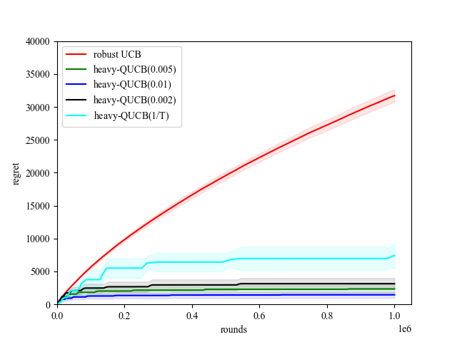
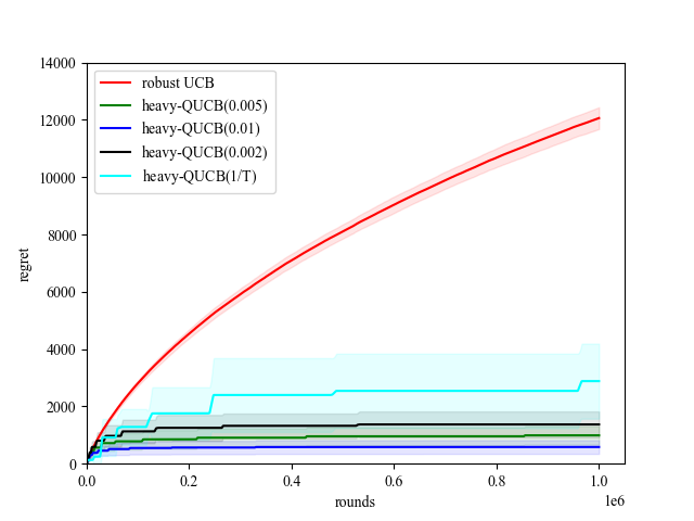
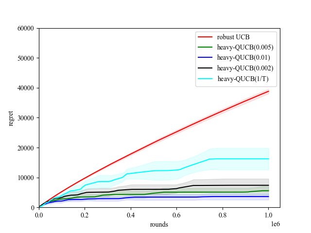
Figure 1: Comparison between robust UCB and Heavy-QUCB with $v=0.5$, Heavy-QUCB ($1/T$) means $\delta=1/T$

The estimator (10) has simple a closed-form solution as follows. Let

$$V_{s}=\lambda I+\sum_{k=1}^{s}\frac{1}{\epsilon_{k}^{2}}a_{k}a_{k}^{\top}=\lambda I+A_{s}^{\top}W_{s}A_{s}\in\mathbb{R}^{d\times d}.$$

Then, $\hat{\theta}_{s}:=V_{s}^{-1}A_{s}^{\top}W_{s}X_{s},$ where $A_{s},X_{s},W_{s}$ are defined in Line 10 in Algorithm 4. It is notable that we need to carefully set $\epsilon_{s}=\left\|a_{s}\right\|_{V_{s-1}^{-1}}$ where $V_{s-1}$ is calculated in epoch $s-1$. This choice makes the determinant of $V_{s}$, $\text{det}(V_{s})$, be double compared with the last epoch. Therefore, Heavy-QLinUCB uses an implicit “doubling trick” which makes the number of epochs be $O(d\log T)$ (Lemma 1), controls the estimation error of $x_{s}$ and $\epsilon_{s}$, and enforces the confidence interval of $\theta^{*}$ to decrease with the epoch increasing (Lemma 2). Specifically, we have the following two lemmas.

Lemma 1.

Algorithm 4 has at most $m=d\log\left(\frac{L^{2}T^{\frac{4v}{1+v}}}{d\lambda}+1\right)$ epochs if $v\in[\frac{1}{3},1]$, where $\lambda$ is the regularization parameter in (10).

Lemma 2.

With probability at least $1-\delta$, for all $s\geq 0,\theta^{*}\in\mathcal{C}_{s}:=\left\{\theta\in\mathbb{R}^{d}:\left\|\theta-\hat{\theta}_{s}\right\|_{V_{s}}\leq\right.$ $\left.\lambda^{1/2}S+\sqrt{ds}\right\}$.

Theorem 5 (Regret bound).

Under the heavy-tailed assumption 4 for rewards with $v\in[\frac{1}{3},1]$, with probability at least $1-\delta$, the upper bound of the expected regret of Algorithm 4, $\mathbb{E}[\mathcal{R}_{T}]$, is $O(d^{2}u^{\frac{1}{1+v}}\log^{\frac{3}{2}}(\frac{L^{2}T^{\frac{4v}{1+v}}}{d\lambda}+1)T^{\frac{1-v}{1+v}}\cdot(\log\frac{d\log(\frac{L^{2}T^{\frac{4v}{1+v}}}{d\lambda}+1)}{\delta})^{\frac{2v}{1+v}}).$

Remark 3.

Note that when $v=1$, we can recover the result in (Wan et al., 2022, Theorem 3) for quantum SLB with bounded rewards. On the other hand, compared with the optimal regret bound of $\Theta(dT^{\frac{1}{1+v}})$ for classical heavy-tailed SLB with infinite arms in Shao et al. (2018), our regret for quantum heavy-tailed SLB with infinite arms in above theorem improves a factor of $\tilde{O}(T^{\frac{v}{1+v}})$ for term $T$.

7 Experiments

In this section, we conduct experiments to demonstrate the performance of our two quantum bandit algorithms. For all experiments, we repeat 100 times and calculate the average regret and the standard deviation. Our experiments are executed on a computer equipped with AMD Ryzen 7 7300X CPU and 16GB memory. Due to the space limit, here we only show partial results for QMAB. Additional results of QMAB and all details for QSLB are shown in Appendix E.

QMAB settings. For the synthetic reward generation, we follow the same settings as in the previous work on (classical) MAB with heavy-tailed rewards Lee et al. (2020); Tao et al. (2022). Specifically, we set $K=5$ and consider three instances $S_{1}$, $S_{2}$, and $S_{3}$, whose reward means all are restricted in the interval $[0.1,1]$: For $S_{1}$ we let the mean gaps of reward distributions of sub-optimal arms decrease linearly where the largest mean is always 0.9 and the smallest mean is always 0.1 (thus the means of rewards in $S_{1}$ are {0.1, 0.3, 0.5, 0.7, 0.9}); In $S_{2}$, we consider an instance that a larger fraction of arms have large sub-optimal gaps, where we set the mean of each arm a by a quadratic convex function $\mu_{a}=0.05(a-5)^{2}+0.1$; In $S_{3}$, we set the mean of each arm $a$ by a concave function $\mu_{a}=-0.05(a-1)^{2}+0.9$. Compared to $S_{2}$, $S_{3}$ has a larger fraction of arms with small sub-optimal gaps. In each instance, the rewards of each arm $i\in[K]$ are sampled from a Pareto distribution with shape parameter $\alpha$ and scale parameter $\lambda_{i}$. We set $\alpha=1.05+v$ which guarantees that the $1+v$-th moment of reward distribution always exists and is upper bounded by $u=\frac{\alpha\lambda_{i}^{1+v}}{\alpha-(1+v)}$ in Equation 3. For a given $\alpha$, the mean is $\frac{\alpha\lambda_{i}}{\alpha-1}$ and this implies $\lambda_{i}=\frac{(\alpha-1)\mu_{i}}{\alpha}$. We take the maximum of $\frac{\alpha\lambda_{i}^{1+v}}{\alpha-(1+v)}$ among all arms as $u$ in Equation 3. We set $v$ to be either 0.2 or 0.5 and fix the number of rounds $T$ as $10^{6}$.

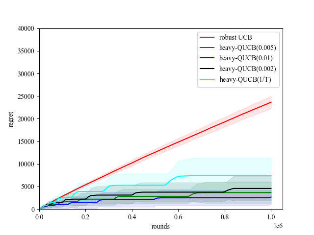
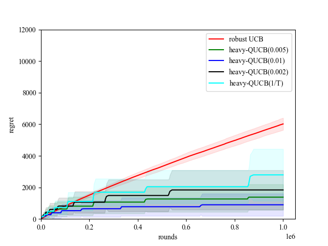
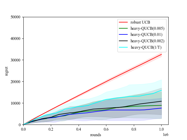
Figure 2: Comparison between robust UCB and Heavy-QUCB with $v=0.2$

Results. To show the superiority of QMAB to the classical MAB, we compare our method with the robust UCB (with $\delta=\frac{1}{T}$) in Bubeck et al. (2013). Besides that, for our method heavy-QUCB, we also consider different failure probabilities $\delta=\{0.005,0.01,0.002,\frac{1}{T}\}$. The results for $v=0.5$ and $v=0.2$ are shown in Figure 1 and Figure 2 in Appendix E, respectively. From the figures, we can see that Heavy-QUCB has much lower expected regret than robust UCB, and such discrepancy becomes more obvious when $v$ becomes larger. This is due to the fact that theoretically we show heavy-QUCB can improve a factor of $\tilde{O}(T^{\frac{v}{1+v}})$. Moreover, for each method we can see larger $v$ will make the expected regret smaller, this is due to that the regret bound is either $\tilde{O}(T^{\frac{1}{1+v}})$ or $\tilde{O}(T^{\frac{1-v}{1+v}})$. Moreover, smaller failure probability will make the regret become larger, which can also be observed in our regret analysis. We can also see similar phenomenons in SLB. In summary, all experimental results corroborate our theories.

8 Conclusions

We investigated the problems of quantum multi-armed bandits (QMAB) and stochastic linear bandits (QSLB) with heavy-tailed rewards. To get a confidence radius of mean estimation of rewards with the quantum reward oracle, we first proposed a novel quantum mean estimation method namely QTME for heavy-tailed random variables which achieves a quadratic improvement on estimation error compared with the classical one. Based on our novel quantum mean estimator, we proposed a UCB-based algorithm named Heavy-QUCB for heavy-tailed MAB with quantum reward oracle and established a regret bound of $\tilde{O}(T^{\frac{1-v}{1+v}})$, where $T$ is the number of rounds. For QSLB, we developed the method of Heavy-QLinUCB based on the Linear UCB framework and show a similar regret bound. Finally, our theoretical results are supported by experimental results, which show the superiority of our algorithms to the classical ones.

Appendix A Useful Lemmas

Lemma 3 (Bernstein’s Inequality Vershynin [2018]).

Let $X_{1},\cdots X_{n}$ be $n$ independent zero-mean random variables. Suppose $|X_{i}|\leq M$ and $\mathbb{E}[X_{i}^{2}]\leq s$ for all $i$. Then for any $t>0$, we have

$$\mathbb{P}\{\frac{1}{n}\sum_{i=1}^{n}X_{i}\geq t\}\leq\exp(-\frac{\frac{1}{2}t^{2}n}{s+\frac{1}{3}Mt})$$

Lemma 4.

Let $f(x)=(\sum_{k=1}^{m}(a_{k})^{x})^{\frac{1}{x}}$ where $a_{k}>0$ and $x\in(0,+\infty)$, then $f(x)$ is a decreasing function on $x$.

Proof of Lemma 4.

Let $g(x)=\ln f(x)=\frac{1}{x}\ln\left(\sum_{k=1}^{m}(a_{k})^{x}\right)$. Then

$$\frac{\mathrm{d}g(x)}{\mathrm{d}x} =-\frac{1}{x^{2}}\ln\left(\sum_{k=1}^{m}(a_{k})^{x}\right)+\frac{1}{x}\frac{\sum_{k=1}^{m}(a_{k})^{x}\ln a_{k}}{\sum_{k=1}^{m}(a_{k})^{x}}$$

$$=\frac{\sum_{k=1}^{m}(a_{k})^{x}\ln(a_{k})^{x}-\sum_{k=1}^{m}(a_{k})^{x}\ln\left(\sum_{k=1}^{m}(a_{k})^{x}\right)}{x^{2}\sum_{k=1}^{m}(a_{k})^{x}}$$

$$=\frac{\sum_{k=1}^{m}(a_{k})^{x}\ln\left(\frac{(a_{k})^{x}}{\sum_{k=1}^{m}(a_{k})^{x}}\right)}{x^{2}\sum_{k=1}^{m}(a_{k})^{x}}$$

$$<0.$$

Thus, we get the result. ∎

Appendix B Omitted Proofs of Section 4

Proof of Theorem 2.

$$|\widehat{\mu}-\mu| \leq\sum^{k}_{\ell=0}a_{\ell}\cdot|\widehat{\mu}_{\ell}-\mu_{\ell}|+\operatorname{\mathbb{E}}[X\cdot\mathbbm{1}_{X>B}]$$

$$\leq\sum^{k}_{\ell=0}\frac{\sqrt{a_{\ell}\cdot\mu_{\ell}}\log(1/\delta)}{t}+\sum^{k}_{\ell=0}\frac{a_{\ell}\log(1/\delta)^{2}}{t^{2}}+\operatorname{\mathbb{E}}[X\cdot\mathbbm{1}_{X>B}]$$

$$\leq\frac{B\log(1/\delta)}{tn}+\sum^{k}_{\ell=1}\frac{\sqrt{2\operatorname{\mathbb{E}}[X^{2}\cdot\mathbbm{1}_{a_{\ell-1<X\leq a_{\ell}}}]}\log(1/\delta)}{t}+\frac{2B\log(1/\delta)^{2}}{t^{2}}+\operatorname{\mathbb{E}}[X\cdot\mathbbm{1}_{X>B}]$$

$$=\frac{B\log(1/\delta)}{cn^{2}\sqrt{\log(1/\delta)}}+\sum^{k}_{\ell=1}\frac{\sqrt{2\operatorname{\mathbb{E}}[X^{2}\cdot\mathbbm{1}_{a_{\ell-1<X\leq a_{\ell}}}]}\log(1/\delta)}{cn\sqrt{\log(1/\delta)}}+\frac{2B\log(1/\delta)^{2}}{c^{2}n^{2}\log(1/\delta)}+\operatorname{\mathbb{E}}[X\cdot\mathbbm{1}_{X>B}]$$

$$\leq\frac{\sqrt{2k}\cdot\sqrt{\sum^{k}_{\ell=1}\operatorname{\mathbb{E}}[X^{2}\cdot\mathbbm{1}_{a_{\ell-1}<X\leq a_{\ell}}]}\cdot\log(1/\delta)}{cn\sqrt{\log(1/\delta)}}+\frac{3B\log(1/\delta)^{2}}{cn^{2}\sqrt{\log(1/\delta)}}+\operatorname{\mathbb{E}}[X\cdot\mathbbm{1}_{X>B}]$$

$$=\frac{\sqrt{2}\cdot\sqrt{\operatorname{\mathbb{E}}[X^{2}\cdot\mathbbm{1}_{|X|\leq B}]}\cdot\log(1/\delta)}{cn}+\frac{3B\log(1/\delta)^{2}}{cn^{2}\sqrt{\log(1/\delta)}}+\operatorname{\mathbb{E}}[X\cdot\mathbbm{1}_{X>B}]$$

$$\leq\frac{\sqrt{2}\cdot\sqrt{uB^{1-v}}\cdot\log(1/\delta)}{cn}+\frac{3B\log(1/\delta)^{2}}{cn^{2}\sqrt{\log(1/\delta)}}+\frac{u}{B^{v}}$$

where the second inequality follows from Bernstein’s inequality in Lemma 3, the third inequality uses $a_{0}\mu_{0}\leq a_{0}^{2}=\frac{B^{2}}{m^{2}}$ and $a_{\ell}\mu_{\ell}\leq 2\operatorname{\mathbb{E}}[X^{2}\cdot\mathbbm{1}_{a_{\ell-1}<X\leq a_{\ell}}]$ when $\ell\geq 1$, the fourth inequality uses the Cauchy-Schwarz inequality, the sixth inequality uses the fact that $\operatorname{\mathbb{E}}[X^{2}\cdot\mathbbm{1}_{|X|\leq B}]\leq uB^{1-v}$ and $\operatorname{\mathbb{E}}[X\cdot\mathbbm{1}_{|X|>B}]\leq\frac{u}{B^{v}}$ when $\operatorname{\mathbb{E}}[|X|^{1+v}\leq u$ and the equalities use the definition of $t$ and $k$.

∎

Proof of Theorem 3.

Using the fact that $X=Y_{+}-Y_{-}$ and taking $B_{t}=\left(\frac{\sqrt{u}t}{\log(1/\delta)}\right)^{\frac{2}{1+v}}$, we obtain that

$$|\widehat{\mu}_{B_{n}}-\mu| \leq|\widehat{\mu}_{Y_{+}}-\mu_{Y_{+}}|+|\widehat{\mu}_{Y_{-}}-\mu_{Y_{-}}|$$

$$\leq\frac{\sqrt{2uB_{n}^{1-v}}\log(1/\delta)}{n}+\frac{3B_{n}\log^{2}(1/\delta)}{n^{2}}+\frac{u}{B_{n}^{v}}$$

$$\leq C\frac{u^{\frac{1}{1+v}}(\log\frac{1}{\delta})^{\frac{2v}{1+v}}}{n^{\frac{2v}{1+v}}}$$

∎

Appendix C Omitted Proofs of Section 5

Proof of Theorem 4.

For each arm $i$, let $\mathcal{S}_{i}$ be the set of stages when arm $i$ is played, and denote $|\mathcal{S}_{i}|=M_{i}$. Initial stages are not included in $\mathcal{S}_{i}$. According to Algorithm 3, each time we find arm $i$ by adopting UCB in Line 7 in some stages, $N_{i}$ is doubled subsequently. Then we play arm $i$ for consecutive $N_{i}$ rounds. This means that the number of rounds of each stage in $\mathcal{S}_{i}$ are $2^{1},2^{2},\dots,2^{M_{i}}$. In total, arm $i$ has been played for $2^{M_{i}+1}-1$ rounds. Because the total number of rounds is at most $T$, we have

$$\sum_{i=1}^{K}\left(2^{M_{i}+1}-1\right)\leq T.$$

Because $2^{x}$ is a convex function in $x\in[0,+\infty)$, by Jensen’s inequality we have

$$\sum_{i=1}^{K}2^{M_{i}+1}\geq K\cdot 2^{\frac{1}{K}\sum_{i=1}^{K}\left(M_{i}+1\right)}$$

Then we have,

$$\sum_{i=1}^{K}M_{i}\leq K\log\left(\frac{T+K}{K}\right)-K.$$

Since QTME is called for $K+\sum_{i=1}^{K}{M_{i}}$ times, by the union bound, with probability at least $1-K\delta\log\frac{T+K}{K}$ the output estimate of every invocation of QTME satisfies (8).We refer to the event as the good event and let $\mathcal{E}$ denote the good event.

Below we assume the good event holds. Recall that $i^{*}$ is the optimal arm and $i_{s}$ is the arm chosen by the algorithm during stage $s$. By the Line 7 of Algorithm 3, we have

$$\hat{\mu}\left(i_{s}\right)+\beta_{i_{s}}\geq\hat{\mu}\left(i^{*}\right)+\beta_{i^{*}}.$$

Under good event,

$${\mu}\left(i_{s}\right)+\beta_{i_{s}}\geq\hat{\mu}\left(i_{s}\right)\quad\text{and}\quad\hat{\mu}\left(i^{*}\right)+\beta_{i^{*}}\geq{\mu}\left(i^{*}\right).$$

Therefore, we obtain

$$\mu\left(i_{s}\right)+2\beta_{i_{s}}\geq\hat{\mu}\left(i_{s}\right)+\beta_{i_{s}}\geq\hat{\mu}\left(i^{*}\right)+\beta_{i^{*}}\geq\mu\left(i^{*}\right),$$

and it follows that

$$\Delta_{i_{s}}:=\mu\left(i^{*}\right)-\mu\left(i_{s}\right)\leq 2\beta_{i_{s}}.$$ (11)

For each arm $i$, we denote by $\mathcal{R}(T;i)$ the contribution of arm $i$ to the cumulative regret over $T$ rounds. By our notation above, arm $i$ is pulled in $M_{i}$ stages and the initialization stage. initialization stages it is pulled for $1$ time. In each stage of $\mathcal{S}_{i}$ it is pulled for $N_{i}=2^{1},\dots,2^{M_{i}}$ times respectively, and the reward gap $\Delta_{i}\leq 2\beta_{i}$ in the last stage is $2C\frac{u^{\frac{1}{1+v}}(\log\frac{1}{\delta})^{\frac{2v}{1+v}}}{2^{\frac{2v}{1+v}M_{i}}}$. Note that the index of the stage in $\mathcal{S}_{i}$ does not influence the gap $\Delta_{i_{s}}$. Therefore, we can use $2C\frac{u^{\frac{1}{1+v}}(\log\frac{1}{\delta})^{\frac{2v}{1+v}}}{2^{\frac{2v}{1+v}M_{i}}}$ to bound the gap of $\mu(i^{*})$ and $\mu(i_{s})$. Thus, we have,

$$\mathcal{R}(T;i) \leq\sum_{m=0}^{M_{i}}2^{m}\cdot 2C\frac{u^{\frac{1}{1+v}}(\log\frac{1}{\delta})^{\frac{2v}{1+v}}}{2^{\frac{2v}{1+v}M_{i}}}$$

$$\leq 4Cu^{\frac{1}{1+v}}(\log\frac{1}{\delta})^{\frac{2v}{1+v}}2^{\frac{1-v}{1+v}M_{i}}$$

$$\leq 4Cu^{\frac{1}{1+v}}(\log\frac{1}{\delta})^{\frac{2v}{1+v}}T^{\frac{1-v}{1+v}}$$

where the last inequality comes from the fact $M_{i}\leq\log T$. The cumulative regret is the summation of $\mathcal{R}(T;i)$ for $i\neq i^{*}$. We have

$$\mathcal{R}_{T}=\sum_{i\neq i^{*}}\mathcal{R}(T;i)\leq 4Cu^{\frac{1}{1+v}}(\log\frac{1}{\delta})^{\frac{2v}{1+v}}(K-1)T^{\frac{1-v}{1+v}}.$$

Since we have good event $\mathcal{E}$ with probability $1-K\delta\log\frac{T+K}{K}$, we can obtain the regret bound by taking $\delta=\frac{1}{T}$

$$\mathbb{E}[\mathcal{R}_{T}]$$

$$\leq \left(1-\frac{K}{T}\log\frac{T+K}{K}\right)\mathbb{E}[[\mathcal{R}_{T}|\mathcal{E}]+\frac{K}{T}\log\frac{T+K}{K}\mathbb{E}[[\mathcal{R}_{T}|\bar{\mathcal{E}}]$$

$$\leq 4Cu^{\frac{1}{1+v}}(\log T)^{\frac{2v}{1+v}}(K-1)T^{\frac{1-v}{1+v}}+$$

$$T\cdot Cu^{\frac{1}{1+v}}(\log T)^{\frac{2v}{1+v}}\frac{K}{T}\log\frac{T+K}{K}$$

$$\leq O\left(u^{\frac{1}{1+v}}KT^{\frac{1-v}{1+v}}\log T\right)$$

∎

Appendix D Omitted Proofs of Section 6

Proof of Lemma 1.

We show that if Algorithm 4 executes $m$ stages, then at least $T$ rounds are played. We first give a lower bound for $\sum_{k=1}^{m}\frac{1}{\epsilon_{k}^{2}}$. For $k\geq 0$,

$$\operatorname{det}\left(V_{k+1}\right)$$

$$=\operatorname{det}\left(V_{k}+\frac{1}{\epsilon_{k+1}^{2}}a_{k+1}a_{k+1}^{\top}\right)$$

$$=\operatorname{det}\left(V_{k}^{1/2}\left(I+\frac{1}{\epsilon_{k+1}^{2}}V_{k}^{-1/2}a_{k+1}a_{k+1}^{\top}V_{k}^{-1/2}\right)V_{k}^{1/2}\right)$$

$$=\operatorname{det}\left(V_{k}\right)\operatorname{det}\left(I+\frac{1}{\epsilon_{k+1}^{2}}V_{k}^{-1/2}a_{k+1}a_{k+1}^{\top}V_{k}^{-1/2}\right)$$

$$=\operatorname{det}\left(V_{k}\right)\left(1+\left\|\frac{1}{\epsilon_{k+1}}V_{k}^{-1/2}a_{k+1}\right\|^{2}\right)$$

$$=\operatorname{det}\left(V_{k}\right)\left(1+\frac{1}{\epsilon_{k+1}^{2}}\left\|a_{k+1}\right\|_{V_{k}^{-1}}^{2}\right)$$

$$=2\operatorname{det}\left(V_{k}\right).$$

Thus,$\operatorname{det}\left(V_{m}\right)=2^{m}\operatorname{det}\left(V_{0}\right)=2^{m}\lambda^{d}$. On the other hand,

$$\operatorname{tr}\left(V_{m}\right)=d\lambda+\sum_{k=1}^{m}\frac{\left\|a_{k}\right\|^{2}}{\epsilon_{k}^{2}}\leq d\lambda+\sum_{k=1}^{m}\frac{L^{2}}{\epsilon_{k}^{2}}.$$

By the trace-determinant inequality,

$$d\lambda+\sum_{k=1}^{m}\frac{L^{2}}{\epsilon_{k}^{2}}\geq\operatorname{tr}\left(V_{m}\right)\geq d\cdot\operatorname{det}\left(V_{m}\right)^{1/d}=d\lambda\cdot 2^{m/d}.$$

Hence,

$$\sum_{k=1}^{m}\frac{1}{\epsilon_{k}^{2}}\geq\frac{d\lambda}{L^{2}}\left(2^{m/d}-1\right).$$

Since the $k$-th stage contains $\frac{Cu^{\frac{1}{2v}}\log(m/\delta)}{\epsilon_{k}^{\frac{1+v}{2v}}}$ rounds, the first $m$ stages contain $\sum_{k=1}^{m}\frac{Cu^{\frac{1}{2v}}\log(m/\delta)}{\epsilon_{k}^{\frac{1+v}{2v}}}$ rounds in total. By the above argument, we have for $v\in[\frac{1}{3},1]$

$$\sum_{k=1}^{m}\frac{Cu^{\frac{1}{2v}}\log(m/\delta)}{\epsilon_{k}^{\frac{1+v}{2v}}} \geq\sum_{k=1}^{m}\frac{1}{\epsilon_{k}^{\frac{1+v}{2v}}}$$

$$\geq\left(\sum_{k=1}^{m}\frac{1}{\epsilon_{k}^{2}}\right)^{\frac{1+v}{4v}}$$

$$\geq\left(\frac{d\lambda}{L^{2}}\left(2^{m/d}-1\right)\right)^{\frac{1+v}{4v}}$$

$$\geq T.$$

where the second inequality follows from Lemma 4 for $v\in[\frac{1}{3},1]$. ∎

Proof of Theorem 5.

In stage $s$, the algorithm plays action $a_{s}$ for $N_{s}=\frac{Cu^{\frac{1}{2v}}\log(m/\delta)}{\epsilon_{s}^{\frac{1+v}{2v}}}$ rounds. The regret in each round is $\left(a^{*}-a_{s}\right)^{\top}\theta^{*}$. By the choice of $\left(a_{s},\tilde{\theta}_{s}\right)$,

$$\left(a^{*}\right)^{\top}\theta^{*}\leq a_{s}^{\top}\tilde{\theta}_{s}.$$

Therefore, by Cauchy-Schwarz inequality,

$$\left(a^{*}-a_{s}\right)^{\top}\theta^{*}$$

$$\leq a_{s}^{\top}\left(\tilde{\theta}_{s}-\theta^{*}\right)\leq\left\|a_{s}\right\|_{V_{s-1}^{-1}}\left\|\tilde{\theta}_{s}-\theta^{*}\right\|_{V_{s-1}}$$

$$\leq\left\|a_{s}\right\|_{V_{s-1}^{-1}}\left(\left\|\tilde{\theta}_{s}-\hat{\theta}_{s-1}\right\|_{V_{s-1}}+\left\|\hat{\theta}_{s-1}-\theta^{*}\right\|_{V_{s-1}}\right)$$

$$=\epsilon_{s}\cdot\left(\left\|\tilde{\theta}_{s}-\hat{\theta}_{s-1}\right\|_{V_{s-1}}+\left\|\hat{\theta}_{s-1}-\theta^{*}\right\|_{V_{s-1}}\right).$$

By the choice of $\tilde{\theta}_{s}$ and Lemma 2, with probability at least $1-\delta$, for all stages $s\geq 1$, both $\tilde{\theta}_{s}$ and ${\theta}^{*}$ lie in $\mathcal{C}_{s-1}$. Thus,

$$\left(a^{*}-a_{s}\right)^{\top}\theta^{*}\leq 2\epsilon_{s}\cdot\left(\lambda^{1/2}S+\sqrt{d(s-1)}\right).$$

The cumulative regret in stage s is therefore bounded by

$$\frac{2Cu^{\frac{1}{2v}}\left(\lambda^{1/2}S+\sqrt{d(s-1)}\right)\log(m/\delta)}{\epsilon_{s}^{\frac{1-v}{2v}}}$$

$$= 2\left(\lambda^{1/2}S+\sqrt{d(s-1)}\right)\left(C\log\frac{m}{\delta}\right)^{\frac{2v}{1+v}}u^{\frac{1}{1+v}}N_{s}^{\frac{1-v}{1+v}}.$$

which follows from the relationship of $N_{s}=\frac{Cu^{\frac{1}{2v}}\log(m/\delta)}{\epsilon_{s}^{\frac{1+v}{2v}}}$.

Since there are at most $m$ stages by Lemma 1, the cumulative regret over all stages and rounds satisfies

$$\mathcal{R}_{T}$$

$$\leq 2\left(\lambda^{1/2}S+\sqrt{d(m-1)}\right)\left(C\log\frac{m}{\delta}\right)^{\frac{2v}{1+v}}u^{\frac{1}{1+v}}\sum_{k=1}^{m}N_{s}^{\frac{1-v}{1+v}}$$

$$\leq 2\left(\lambda^{1/2}S+\sqrt{d(m-1)}\right)\left(C\log\frac{m}{\delta}\right)^{\frac{2v}{1+v}}u^{\frac{1}{1+v}}mT^{\frac{1-v}{1+v}}$$

$$\leq O\left(\left(\lambda^{1/2}Sm+{d^{\frac{1}{2}}m^{\frac{3}{2}}}\right)\left(\log\frac{m}{\delta}\right)^{\frac{2v}{1+v}}u^{\frac{1}{1+v}}T^{\frac{1-v}{1+v}}\right)$$

$$\leq O\left(d^{2}u^{\frac{1}{1+v}}T^{\frac{1-v}{1+v}}\log^{3/2}\left(\frac{L^{2}T^{\frac{4v}{1+v}}}{d\lambda}+1\right)\right.$$

$$\quad\cdot\left.\left(\log\frac{d\log\left(\frac{L^{2}T^{\frac{4v}{1+v}}}{d\lambda}+1\right)}{\delta}\right)^{\frac{2v}{1+v}}\right)$$

For expected regret bound, let $\mathcal{E}$ be the event that the above bound holds. Note that for any $a_{1},a_{2}\in\mathcal{A}$,

$$\left|\left(a_{1}-a_{2}\right)^{\top}\theta^{*}\right| \leq\left\|a_{1}-a_{2}\right\|_{2}\left\|\theta^{*}\right\|_{2}$$

$$\leq\left(\left\|a_{1}\right\|_{2}+\left\|a_{2}\right\|\right)\left\|\theta^{*}\right\|_{2}$$

$$\leq 2LS.$$

Then, by taking $\delta=\frac{1}{T}$ we have

$$\mathbb{E}[\mathcal{R}_{T}]$$

$$= \mathbb{E}[\mathcal{R}_{T}\mid\mathcal{E}]\operatorname{Pr}[\mathcal{E}]+\mathbb{E}[R(T)\mid\overline{\mathcal{E}}]\operatorname{Pr}[\overline{\mathcal{E}}]$$

$$\leq O\left(\left(\lambda^{1/2}Sm+{d^{\frac{1}{2}}m^{\frac{3}{2}}}\right)\left(\log\frac{m}{\delta}\right)^{\frac{2v}{1+v}}u^{\frac{1}{1+v}}T^{\frac{1-v}{1+v}}\right)+2LST\frac{m}{T}$$

$$= O\left(d^{2}u^{\frac{1}{1+v}}T^{\frac{1-v}{1+v}}\log^{3/2}\left(\frac{L^{2}T^{\frac{4v}{1+v}}}{d\lambda}+1\right)\cdot\left(\log\frac{d\log\left(\frac{L^{2}T^{\frac{4v}{1+v}}}{d\lambda}+1\right)}{\delta}\right)^{\frac{2v}{1+v}}\right)$$

where we omit $\log\log(\cdot)$ term. ∎

Appendix E More Numerical Experiments

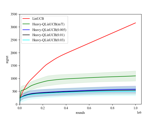
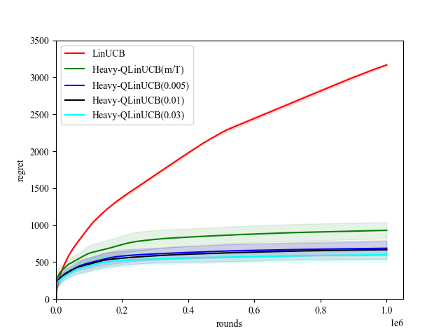
Figure 3: Simulation for the QSLB setting with different $\delta$

Simulation of quantum mean estimator. As mentioned in Wan et al. [2022], the closed form of the measurement output distribution given in Theorem 11 of Brassard et al. [2002] enables a classical way to the simulation of quantum amplitude estimation algorithm. We use this strategy to simulate our quantum mean estimator.

QSLB setting. For this setting, we set $T=10^{6}$ and study 3 instances: (1) $\theta^{*}_{1}=(\cos(0.35\pi),\sin(0.35\pi))$ as in Wan et al. [2022]; (2) $\theta^{*}_{2}=(\cos(\pi/6),\sin(\pi/6))$; (3) $\theta^{*}_{3}=(\cos(5\pi/6),\sin(5\pi/6))$. As for the action set, we use a finite one that consists of 50 actions equally spaced on the positive part of the unit circle.

As for the solver for $(a_{s},\tilde{\theta}_{s})$ in Algorithm 4, there is no efficient solver in general. However, when considering the finite action set, a straightforward approach to solving this is to enumerate all possible solutions in a small finite set. The existence of a small finite solution set with high probability is shown by Lemma 2 and hence, this enables the feasibility of using enumeration on solving for $(a_{s},\tilde{\theta}_{s})$. Following a similar idea in Wan et al. [2022], the upper bound on $\|\theta-\hat{\theta}_{s-1}\|_{V_{s-1}}$ can be calculated. For completeness, $\|\theta-\hat{\theta}_{s-1}\|_{V_{s-1}}\leq\lambda^{1/2}S+\sqrt{(s-1)\|W^{1/2}_{s-1}A_{s-1}V^{-1}_{s-1}A^{\top}_{s-1}W^{1/2}_{s-1}\|_{2}}$.

We compare our algorithm with the well-known LinUCB Lattimore and Szepesvári [2020] for the case $v=1$ and $\lambda=1$, which is shown in Figure 3. From the results, we can see that Heavy-QLinUCB has lower regret than LinUCB. By comparison with QLinUCB in Wan et al. [2022] on the first instance $\theta^{*}_{1}$, we can also observe that Heavy-QlinUCB has slightly better performance which matches the comparison in Table 1.

References

• Abrams and Williams [1999] Daniel S Abrams and Colin P Williams. Fast quantum algorithms for numerical integrals and stochastic processes. arXiv preprint quant-ph/9908083, 1999.
• Agrawal [1995] Rajeev Agrawal. Sample mean based index policies by o (log n) regret for the multi-armed bandit problem. Advances in Applied Probability, 27(4):1054–1078, 1995.
• Auer et al. [2002] Peter Auer, Nicolo Cesa-Bianchi, and Paul Fischer. Finite-time analysis of the multiarmed bandit problem. Machine learning, 47(2):235–256, 2002.
• Azize and Basu [2022] Achraf Azize and Debabrota Basu. When privacy meets partial information: A refined analysis of differentially private bandits. arXiv preprint arXiv:2209.02570, 2022.
• Bradley and Taqqu [2003] Brendan O Bradley and Murad S Taqqu. Financial risk and heavy tails. In Handbook of heavy tailed distributions in finance, pages 35–103. Elsevier, 2003.
• Brassard et al. [2002] Gilles Brassard, Peter Hoyer, Michele Mosca, and Alain Tapp. Quantum amplitude amplification and estimation. Contemporary Mathematics, 305:53–74, 2002.
• Brassard et al. [2011] Gilles Brassard, Frederic Dupuis, Sebastien Gambs, and Alain Tapp. An optimal quantum algorithm to approximate the mean and its application for approximating the median of a set of points over an arbitrary distance. arXiv preprint arXiv:1106.4267, 2011.
• Bubeck et al. [2013] Sébastien Bubeck, Nicolo Cesa-Bianchi, and Gábor Lugosi. Bandits with heavy tail. IEEE Transactions on Information Theory, 59(11):7711–7717, 2013.
• Casalé et al. [2020] Balthazar Casalé, Giuseppe Di Molfetta, Hachem Kadri, and Liva Ralaivola. Quantum bandits. Quantum Machine Intelligence, 2(1):1–7, 2020.
• Cohen et al. [2020] Maxime C Cohen, Ilan Lobel, and Renato Paes Leme. Feature-based dynamic pricing. Management Science, 66(11):4921–4943, 2020.
• Grover [1998] Lov K Grover. A framework for fast quantum mechanical algorithms. In Proceedings of the thirtieth annual ACM symposium on Theory of computing, pages 53–62, 1998.
• Gutiérrez et al. [2017] Benjamín Gutiérrez, Loïc Peter, Tassilo Klein, and Christian Wachinger. A multi-armed bandit to smartly select a training set from big medical data. In International Conference on Medical Image Computing and Computer-Assisted Intervention, pages 38–45. Springer, 2017.
• Hamoudi [2021] Yassine Hamoudi. Quantum sub-gaussian mean estimator. arXiv preprint arXiv:2108.12172, 2021.
• Heinrich [2002] Stefan Heinrich. Quantum summation with an application to integration. Journal of Complexity, 18(1):1–50, 2002.
• Kumar and Tomkins [2010] Ravi Kumar and Andrew Tomkins. A characterization of online browsing behavior. In Proceedings of the 19th international conference on World wide web, pages 561–570, 2010.
• Lattimore and Szepesvári [2020] Tor Lattimore and Csaba Szepesvári. Bandit algorithms. Cambridge University Press, 2020.
• Lee et al. [2020] Kyungjae Lee, Hongjun Yang, Sungbin Lim, and Songhwai Oh. Optimal algorithms for stochastic multi-armed bandits with heavy tailed rewards. Advances in Neural Information Processing Systems, 33:8452–8462, 2020.
• Lu et al. [2019] Shiyin Lu, Guanghui Wang, Yao Hu, and Lijun Zhang. Optimal algorithms for lipschitz bandits with heavy-tailed rewards. In International Conference on Machine Learning, pages 4154–4163. PMLR, 2019.
• Lumbreras et al. [2022] Josep Lumbreras, Erkka Haapasalo, and Marco Tomamichel. Multi-armed quantum bandits: Exploration versus exploitation when learning properties of quantum states. Quantum, 6:749, 2022.
• Medina and Yang [2016] Andres Munoz Medina and Scott Yang. No-regret algorithms for heavy-tailed linear bandits. In International Conference on Machine Learning, pages 1642–1650. PMLR, 2016.
• Montanaro [2015] Ashley Montanaro. Quantum speedup of monte carlo methods. Proceedings of the Royal Society A: Mathematical, Physical and Engineering Sciences, 471(2181):20150301, 2015.
• Ray Chowdhury and Gopalan [2019] Sayak Ray Chowdhury and Aditya Gopalan. Bayesian optimization under heavy-tailed payoffs. Advances in Neural Information Processing Systems, 32, 2019.
• Ruotsalainen et al. [2018] Laura Ruotsalainen, Martti Kirkko-Jaakkola, Jesperi Rantanen, and Maija Mäkelä. Error modelling for multi-sensor measurements in infrastructure-free indoor navigation. Sensors, 18(2):590, 2018.
• Shao et al. [2018] Han Shao, Xiaotian Yu, Irwin King, and Michael R Lyu. Almost optimal algorithms for linear stochastic bandits with heavy-tailed payoffs. Advances in Neural Information Processing Systems, 31, 2018.
• Tang et al. [2013] Liang Tang, Romer Rosales, Ajit Singh, and Deepak Agarwal. Automatic ad format selection via contextual bandits. In Proceedings of the 22nd ACM international conference on Information & Knowledge Management, pages 1587–1594, 2013.
• Tao et al. [2022] Youming Tao, Yulian Wu, Peng Zhao, and Di Wang. Optimal rates of (locally) differentially private heavy-tailed multi-armed bandits. In International Conference on Artificial Intelligence and Statistics, pages 1546–1574. PMLR, 2022.
• Terhal [1999] Barbara Terhal. Quantum algorithms and quantum entanglement. PhD thesis, University of Amsterdam, 1999.
• Thompson [1933] William R Thompson. On the likelihood that one unknown probability exceeds another in view of the evidence of two samples. Biometrika, 25(3-4):285–294, 1933.
• Vershynin [2018] Roman Vershynin. High-dimensional probability: An introduction with applications in data science, volume 47. Cambridge university press, 2018.
• Wan et al. [2022] Zongqi Wan, Zhijie Zhang, Tongyang Li, Jialin Zhang, and Xiaoming Sun. Quantum multi-armed bandits and stochastic linear bandits enjoy logarithmic regrets. arXiv preprint arXiv:2205.14988, 2022.
• Wang et al. [2021a] Daochen Wang, Aarthi Sundaram, Robin Kothari, Ashish Kapoor, and Martin Roetteler. Quantum algorithms for reinforcement learning with a generative model. In International Conference on Machine Learning, pages 10916–10926. PMLR, 2021.
• Wang et al. [2021b] Daochen Wang, Xuchen You, Tongyang Li, and Andrew M Childs. Quantum exploration algorithms for multi-armed bandits. In Proceedings of the AAAI Conference on Artificial Intelligence, volume 35, pages 10102–10110, 2021.
• Xue et al. [2020] Bo Xue, Guanghui Wang, Yimu Wang, and Lijun Zhang. Nearly optimal regret for stochastic linear bandits with heavy-tailed payoffs. arXiv preprint arXiv:2004.13465, 2020.
• Yu et al. [2018] Xiaotian Yu, Han Shao, Michael R Lyu, and Irwin King. Pure exploration of multi-armed bandits with heavy-tailed payoffs. In UAI, 2018.