DiffSDS: A language diffusion model for protein backbone inpainting under geometric conditions and constraints

Abstract

Have you ever been troubled by the complexity and computational cost of SE(3) protein structure modeling and been amazed by the simplicity and power of language modeling? Recent work has shown promise in simplifying protein structures as sequences of protein angles; therefore, language models could be used for unconstrained protein backbone generation. Unfortunately, such simplification is unsuitable for the constrained protein inpainting problem, where the model needs to recover masked structures conditioned on unmasked ones, as it dramatically increases the computing cost of geometric constraints. To overcome this dilemma, we suggest inserting a hidden atomic direction space (ADS) upon the language model, converting invariant backbone angles into equivalent direction vectors and preserving the simplicity, called Seq2Direct encoder ($\text{Enc}_{s2d}$). Geometric constraints could be efficiently imposed on the newly introduced direction space. A Direct2Seq decoder ($\text{Dec}_{d2s}$) with mathematical guarantees is also introduced to develop a SDS ($\text{Enc}_{s2d}$+$\text{Dec}_{d2s}$) model. We apply the SDS model as the denoising neural network during the conditional diffusion process, resulting in a constrained generative model–DiffSDS. Extensive experiments show that the plug-and-play ADS could transform the language model into a strong structural model without loss of simplicity. More importantly, the proposed DiffSDS outperforms previous strong baselines by a large margin on the task of protein inpainting.

1 Introduction

We aim to improve and simplify the modeling of constrained protein backbone inpainting, i.e., recovering masked protein backbones, which has wide applications in de-novo protein design (Wang et al., 2022a; Lee & Kim, 2022; Ferruz et al., 2022). Since the milestone breakthrough of AlphaFold (Jumper et al., 2021), protein structure models are becoming increasingly sophisticated, including the introduction of equivalent learning biases, geometric interactions, and fine-grained structure modules (Ganea et al., 2021b; Jin et al., 2021; Luo et al., ; Lee & Kim, 2022; Wang et al., 2022a; Trippe et al., 2022; Anand & Achim, 2022). These improvements achieve significant success in structure modeling; however, the additional computational overhead and complexity have also troubled researchers. Despite the complexity of protein structure modeling, language transformers seem to unify everything for more difficult NLP tasks while enjoying good efficiency and simplicity. Can we convert constrained protein structure design as a sequence modeling task and thus apply language models for simplification?

Existing protein structural generative models explicitly consider the equivalence caused by rotation and translation (Wang et al., 2022a; Trippe et al., 2022; Luo et al., ; Anand & Achim, 2022). These considerations enable them to correctly consider atom interactions in the 3D space while requiring special model designs that increase the complexity and computational cost. Restricted by the equivalence, traditional powerful models, such as visual CNNs or language converters, are prevented from being directly applied to structure modeling. Beyond this limitation, recent FoldingDiff (Wu et al., 2022a) suggests converting protein structures into sequences of angles. Thus, language models could be used for unconditional protein backbone generation.

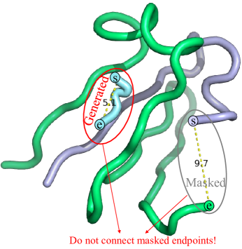
Figure 1: Example of violating geometric constraints, where endpoints $s$ and $e$ are not connected. The inputs are fixed unmasked atoms (colored with green), where atoms between endpoints $s$ and $e$ are masked and should be recovered by the algorithm.

Unfortunately, the pure language model is unsuitable for constrained structure design tasks. In protein backbone inpainting, the designed structure should fit multiple geometric constraints, including linking the masked structure’s endpoints and not overlapping with unmasked structures to meet the repulsion (Spassov et al., 2007; Müller-Späth et al., 2010; Drake & Pettitt, 2020). If the above constraints are not guaranteed, the generated structure will be meaningless, as shown in Fig.1. An open research question is how to efficiently impose geometric constraints on the language model while keeping simplicity.

We suggest inserting a hidden atomic direction space (ADS) into the language model, allowing to impose structural constraints on the novel direction space efficiently. ADS is a plug-and-play cross-modal conversion technique connecting the sequence and direction space. By adding ADS upon the last transformer layer, we obtain the Seq2Direct encoder ($\text{Enc}_{\text{s2d}}$) that converts sequential features into direction vectors. We also introduce Direct2Seq decoder ($\text{Dec}_{\text{d2s}}$) according to strict mathematical transformations. A language model (SDS) equipped with hidden direction space could be constructed by stacking $\text{Enc}_{\text{s2d}}$ and $\text{Dec}_{\text{d2s}}$. SDS takes angular sequences as inputs and outputs, with a latent direction space that supports efficient geometric calculations and is mathematically consistent with the sequence space. In this design, multimodal constraints, e.g., sequential and 3D constraints, can be simultaneously considered on the corresponding feature space. Finally, we apply the SDS model as the denoising neural network during the conditional diffusion process, resulting in a constrained generative model–DiffSDS.

We evaluated DiffSDS on CATH4.3 and compared it with recent strong baselines, including RFDesign (Wang et al., 2022a) and modified FoldingDiff (Wu et al., 2022a). We also propose three metrics to evaluate the results of protein backbone inpainting, including protein likeness, connectivity, and non-overlapping. Experiments show that our methods significantly outperform baselines in all metrics. In addition, the designability of structures generated by DiffSDS is also better than baselines. As to simplicity, the proposed DiffSDS utilizes the language transformer to model protein structures, avoiding the equivalence consideration when constructing neural modules. To provide a deeper understanding, we have also performed ablation studies to reveal the role of conditions and constraints.

1.1 Related work

Problem Definition

Protein backbone inpainting aims to recover the continuous masked substructure of the protein backbone, given the unmasked atoms as conditions. The generated structure is required to connect different protein fragments with fixed spatial positions. Formally, we write the protein backbone as $\mathcal{B}=\{\bm{p}^{C}_{1},\bm{p}^{A}_{1},\bm{p}^{N}_{1},\bm{p}^{C}_{2},\bm{p}^{A}_{2},\bm{p}^{N}_{2},\cdots,\bm{p}^{C}_{n},\bm{p}^{A}_{n},\bm{p}^{N}_{n}\}$, where $\{\bm{p}^{C}_{i},\bm{p}^{A}_{i},\bm{p}^{N}_{i}\}$ indicates the set of backbone atoms ($C$, $C_{\alpha}$ and $N$) of the $i$-th residue and $\bm{p}^{A}_{i}$ is the 3D position of the $i$-th $C_{\alpha}$. Denote the masked sub-structure as $\mathcal{M}=\{\bm{p}^{C}_{i},\bm{p}^{A}_{i},\bm{p}^{N}_{i}\}_{i=s}^{e}$, the unmasked structures as $\mathcal{K}=\{\bm{p}^{C}_{i},\bm{p}^{A}_{i},\bm{p}^{N}_{i}\}_{i=1}^{s-1}\cup\{\bm{p}^{C}_{i},\bm{p}^{A}_{i},\bm{p}^{N}_{i}\}_{i=e+1}^{n}$, where $0<l<r<n$. We generate $\hat{\mathcal{M}}$ connecting endpoints $\bm{p}^{N}_{s-1}$ and $\bm{p}^{C}_{r+1}$ via a learnable function $f_{\theta}$, given $mathcal{U}$ with a fixed conformation as input:

$$\hat{\mathcal{M}}=f_{\theta}(\bm{p}|\mathcal{U},x),x\sim\mathcal{N}(0,\mathbf{I})$$ (1)

Note that $\theta$ indicates learnable parameters. The designed $\hat{\mathcal{M}}$ should be non-trivial to satisfy the following constraints:

1. Protein likeness: The designed structures are likely to constitute natural proteins.

2. Connectivity: $\hat{\mathcal{M}}$ should effectively connect $\bm{p}^{N}_{s-1}$ and $\bm{p}^{C}_{e+1}$ without breakage.

3. Non-overlapping: The designed structure $\hat{\mathcal{M}}$ should not overlap with existing structure $\mathcal{U}$.

3D Molecule Generation

Generating 3D molecules to explore the local minima of the energy function (Conformation Generation) (Gebauer et al., 2019; Simm et al., 2020b, a; Shi et al., 2021; Xu et al., 2021; Luo et al., 2021; Xu et al., 2020; Ganea et al., 2021a; Xu et al., 2022; Hoogeboom et al., 2022; Jing et al., 2022; Zhu et al., 2022) or discover potential drug molecules binding to targeted proteins (3D Drug Design) (Imrie et al., 2020; Nesterov et al., 2020; Luo et al., 2022; Ragoza et al., 2022; Wu et al., 2022b; Huang et al., 2022a; Peng et al., 2022; Huang et al., 2022b; Wang et al., 2022b; Liu et al., 2022b) have attracted extensive attention in recent years. Compared to conformation generation that aims to predict the set of favourable conformers from the molecular graph, 3D Drug Design is more challenging in two aspects: (1) both conformation and molecule graph need to be generated, and (2) the generated molecules should satisfy multiple constraints, such as physical prior and protein-ligand binding affinity. We summarized representive works of 3D drug design in Table.5 in the appendix, where all the methods focus on small molecule design.

Protein Design

In addition to small molecules, biomolecules such as proteins have also attracted considerable attention by researchers (Ding et al., 2022; Ovchinnikov & Huang, 2021; Gao et al., 2020; Strokach & Kim, 2022). We divide the mainstream protein design methods into three categories: protein sequence design (Li et al., 2014; Wu et al., 2021; Pearce & Zhang, 2021; Ingraham et al., 2019; Jing et al., 2020; Tan et al., 2022; Gao et al., 2022a; Hsu et al., 2022; Dauparas et al., 2022; Gao et al., 2022b; O’Connell et al., 2018; Wang et al., 2018; Qi & Zhang, 2020; Strokach et al., 2020; Chen et al., 2019; Zhang et al., 2020; Anand & Achim, 2022), unconditional protein structure generation (Anand & Huang, 2018; Sabban & Markovsky, 2020; Eguchi et al., 2022; Wu et al., 2022a), and conditional protein design (Lee & Kim, 2022; Wang et al., 2022a; Trippe et al., 2022; Lai et al., 2022; Fu & Sun, 2022; Tischer et al., 2020; Anand & Achim, 2022; Luo et al., ). Protein sequence design aims to discover protein sequences folding into the desired structure, and unconditional protein structure generation focus on generating new protein structures from noisy inputs. We are interested in conditional protein design and consider multiple constraints on the designed protein. For example, Wang’s model (Wang et al., 2022a), SMCDiff (Trippe et al., 2022) and Tischer’s model (Tischer et al., 2020) design the scaffold for the specified functional sites. ProteinSGM (Lee & Kim, 2022) mask short spans ($<8$ residues) of different secondary structures in different structures and treats the design task as a inpainting problem. CoordVAE (Lai et al., 2022) produces novel protein structures conditioned on the backbone template. RefineGNN (Jin et al., 2021), CEM (Fu & Sun, 2022), and DiffAb (Luo et al., ) aim to generate the complementarity-determining regions of the antibody. We summarized protein design model in Table.6.

Language Diffusion for Protein Structure Generation

Diffusion models (Sohl-Dickstein et al., 2015; Ho et al., 2020; Cao et al., 2022) are a class of generative models that have achieved impressive results in image (Song et al., 2020; Lugmayr et al., 2022; Whang et al., 2022; Baranchuk et al., 2021; Wolleb et al., 2022), speech (Lee & Han, 2021; Chen et al., 2020; Kong et al., 2020; Liu et al., 2022a) and text (Li et al., 2022; Chen et al., 2022; Austin et al., 2021) synthesis. Recently, FoldingDiff (Wu et al., 2022a) shows that language models could be used for unconditional protein generation.

2 Background and Knowledge Gap

Considering three backbone atoms ($N,C_{\alpha},C$) for each residue, there are 9 ($=3\times 3$) freedom degrees are required for 3D representation. Recently, researchers have introduced human knowledge into protein backbone representation and proposed two simplified approaches: frame-based and angle-based representation, as shown in Fig.2 (a).

Frame-based

This approach treats residues as fundamental elements and assumes that residues of the same type have the same rigid structure, called the local frame. As shown in Fig.2 (a), we write $F_{i}=\{C_{i},C_{\alpha_{i}},N_{i}\}$ as the local frame of the $i$-th residue, where position $\bm{p}_{F_{i}}$, orientation $R_{i}$ and the residue type $s_{i}$ are required for describing $F_{i}$, resulting in 7($=3+3+1$) freedom degrees. Under this representation, geometric features can be computed efficiently, e.g., pairwise distance and relative positions. However, the model needs to consider the geometric equivariance of the input data, which introduces considerable modeling complexity.

Angle-based

This approach converts structures into sequences of backbone angles based on the order of the protein’s primary structure; see Fig.2 (a). By assuming the backbone bond lengths are fixed, three bond angles $\alpha^{N}_{i},\alpha^{A}_{i},\alpha^{C}_{i}$ and three torsion angles $\beta^{N}_{i},\beta^{A}_{i},\beta^{C}_{i}$ are required for describing one residue, leading to 6 freedom degrees. The reduced freedom forms a more compact representation than the frame-based approach. In addition, there is no need to consider geometric equivariance since all angles are invariant to spatial rotation and translation.

Knowledge Gap

The angle-based representation seems attractive for simplifying structural modeling and learning more compact protein representations. However, it suffers from the drawback of inefficient computing of geometric features, making it challenging to consider geometric constraints. For example, if one wants to optimize

$$\mathcal{L}_{dist}=\min_{\{\alpha^{N}_{i},\alpha^{A}_{i},\alpha^{C}_{i},\beta^{N}_{i},\beta^{A}_{i},\beta^{C}_{i}\}_{0}^{i}}(||\bm{p}^{A}_{i}-\bm{p}^{A}_{1}||-r)^{2}$$ (2)

given $\bm{p}^{N}_{1},\bm{p}^{A}_{1},\bm{p}^{C}_{1}$. Then, $\bm{p}^{N}_{2}\rightarrow\bm{p}^{A}_{2}\rightarrow\bm{p}^{C}_{2}\rightarrow\bm{p}^{N}_{3}\rightarrow\bm{p}^{A}_{3}\rightarrow\cdots\rightarrow\bm{p}^{A}_{i}$ needs to be recursively computed by

$$\begin{cases}\bm{p}^{N}_{i}=\text{Place}(\bm{p}^{C}_{i-1},\alpha^{N}_{i-1},\beta^{N}_{i-1},\bm{d}^{C}_{i-1},\bm{d}^{A}_{i-1},r^{N})\\ \bm{p}^{A}_{i}=\text{Place}(\bm{p}^{N}_{i},\alpha^{A}_{i},\beta^{A}_{i-1},\bm{d}^{N}_{i},\bm{d}^{C}_{i-1},r^{A})\\ \bm{p}^{C}_{i}=\text{Place}(\bm{p}^{A}_{i},\alpha^{C}_{i},\beta^{C}_{i},\bm{d}^{A}_{i},\bm{d}^{N}_{i},r^{C})\end{cases}$$ (3)

where $\bm{d}^{N}_{i}=\frac{\bm{p}^{N}_{i}-\bm{p}^{C}_{i-1}}{||\bm{p}^{N}_{i}-\bm{p}^{C}_{i-1}||},\bm{d}^{A}_{i}=\frac{\bm{p}^{A}_{i}-\bm{p}^{N}_{i}}{||\bm{p}^{A}_{i}-\bm{p}^{N}_{i}||},\bm{d}^{C}_{i}=\frac{\bm{p}^{C}_{i}-\bm{p}^{A}_{i}}{||\bm{p}^{C}_{i}-\bm{p}^{A}_{i}||}$. Note that backbone bond lengths, e.g., $r^{N}=||\bm{p}^{N}_{i}-\bm{p}^{C}_{i-1}||,r^{A}=||\bm{p}^{A}_{i}-\bm{p}^{N}_{i}||,r^{C}=||\bm{p}^{C}_{i}-\bm{p}^{A}_{i}||$, are constants. Alg.1 (in the appendix) shows the details of $\text{place}(\bm{p},\alpha,\beta,\bm{d}_{1},\bm{d}_{2})$. Such recursive computation is inefficient, especially for diffusion models, where the training ($>$15 min/epoch) and generating ($>$1h) overhead is unacceptable. Considering the huge computing overhead, the language model is no longer a simple solution for protein structure design under geometric constraints.

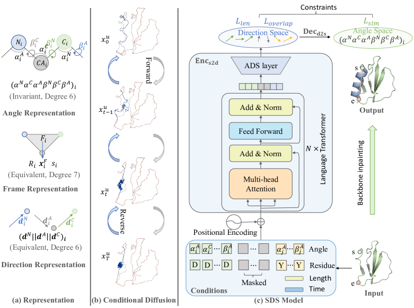
Figure 2: The overall framework. (a) We introduce a new direction representation for efficiently computing geometric features while enjoying minimal freedom. (b) Only the masked structures are involved in the diffusion process, while the unmasked ones remain fixed. (c) We add an ADS layer upon the language transformer to convert invariant features into equivalent directions, namely $\text{Enc}_{\text{s2d}}$. Then the $\text{Dec}_{\text{d2s}}$ reverses directions as invariant features based on Eq.6. The geometric constraints ($\mathcal{L}_{len}$ and $\mathcal{L}_{overlap}$) could be efficiently imposed on the direction space. The overall $\text{Enc}_{\text{s2d}}+\text{Dec}_{\text{d2s}}$ is a simple language model.

3 Method

3.1 Overall Framework

We propose DiffSDS, inserting direction space into the language diffusion model, to serve as a simple solution for constrained protein backbone inpainting. Specifically, the model takes unmasked atoms and controllable conditions as input to recover the masked region, as shown in Fig.2. Compared to previous backbone inpainting methods, our innovations include the following:

1. Inserting direction space into the language model to for simplying the modeling of geometric constraints.

2. Proposing the first language diffusion model for backbone inpainting and a new modeling perspective.

3. Introducing geometric conditions and constraints for protein inpainting.

4. Refining the evaluation metrics, based on which we benchmarked the proposed method and baselines.

3.2 Direction-based Backbone Representation

Direction-based Representation

Is there an alternative representation beyond frame- and angle-based ones to support efficient computation of geometric features while enjoying low degrees of freedom? As shown in Fig.2(a), we introduce direction vectors, i.e., $\bm{d}^{A}_{i},\bm{d}^{N}_{i},\bm{d}^{C}_{i}$, for discribing protein structures. In the direction-based representation, the position of each atom is determined by its relative direction ($\bm{d}^{A}_{i},\bm{d}^{N}_{i},\bm{d}^{C}_{i}$) and distance ($r^{N},r^{A},r^{C}$) from its parent node. In Fig.2(a), taking $C_{\alpha}$ as an example,

$$\bm{p}^{A}_{i}=\bm{p}^{N}_{i}+r^{A}\bm{d}^{A}_{i}$$ (4)

Recall that $\bm{p}^{A}_{i}$ and $\bm{p}^{N}_{i}$ are spatial coordinates of $C_{\alpha_{i}}$ and $N_{i}$. The direction vector $\bm{d}^{A}_{i}$ points from $\bm{p}^{N}_{i}$ to $\bm{p}^{A}_{i}$, and $r^{A}$ is the length of the $C_{\alpha}-C$ bond.

Advantages

The propsed representation has several advantages. Firstly, the computing cost of relative positions will be greatly reduced. For example, when computing $\bm{p}^{A}_{i}-\bm{p}^{A}_{0}$, only parallel linear additions and multiplications are required, without recursive computation as in Eq.3:

$$\bm{p}^{A}_{i}-\bm{p}^{A}_{0}=r^{A}\sum_{k=1}^{i}\bm{d}^{A}_{i}+r^{C}\sum_{k=1}^{i-1}\bm{d}^{C}_{i}+r^{N}\sum_{k=2}^{i}\bm{d}^{N}_{i}$$ (5)

Secondly, this representation enjoys the lowest 6 freedom degrees since $||\bm{d}^{A}_{i}||=||\bm{d}^{C}_{i}||=||\bm{d}^{N}_{i}||=1$. The direction representation could be equivalently transformed to the angle-based one:

$$\begin{cases}\alpha^{N}_{i}=\arccos(-(\bm{d}^{N}_{i+1})^{T}\bm{d}^{C}_{i})\\ \alpha^{A}_{i}=\arccos(-(\bm{d}^{A}_{i})^{T}\bm{d}^{N}_{i})\\ \alpha^{C}_{i}=\arccos(-(\bm{d}^{C}_{i})^{T}\bm{d}^{A}_{i})\\ \beta^{N}_{i}=\text{dihedral}(\bm{d}^{A}_{i},\bm{d}^{C}_{i},\bm{d}^{N}_{i+1})\\ \beta^{A}_{i}=\text{dihedral}(\bm{d}^{C}_{i},\bm{d}^{N}_{i+1},\bm{d}^{A}_{i+1})\\ \beta^{C}_{i}=\text{dihedral}(\bm{d}^{N}_{i},\bm{d}^{A}_{i},\bm{d}^{C}_{i})\end{cases}$$ (6)

where $\text{dihedral}(\bm{v}_{1},\bm{v}_{2},\bm{v}_{3})$ is defined in Alg.2 (Appendix).

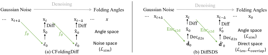
Figure 3: Reverse diffusion. (a) FoldingDiff uses the neural model $f_{\theta}$ to predict one-step noise, where angular similarity loss is imposed on the noise space. We extend FoldingDiff to conditional scenes by fixing the unmasked structure during diffusion to obtain CFoldingDiff. (b) DiffSDS uses $\text{Enc}_{\text{s2d}}$ to predict the direction representation of the original protein. The angular similarity loss and geometric constraints are imposed in the angle and direction space, respectively.

3.3 Conditional language diffusion model equipped with direction space

We propose a language diffusion model $f_{\theta}$ equipped with direction space for recovering masked backbone $\mathcal{M}$ conditional on the unmasked part $\mathcal{U}$:

$$\hat{\mathcal{M}}=f_{\theta}(\bm{p}|\mathcal{U},x),x\sim\mathcal{N}(0,\mathbf{I})$$ (7)

Conditions

The model takes multiple prior conditions as input features for each residue, as shown in Fig.2(c). The node features include backbone angles $F_{ang}\in\mathbb{R}^{n,6}$, and residue type embedding $F_{res}\in\mathbb{R}^{n,20}$. In addition, the global controllable features include the length ($F_{len}\in\mathbb{R}$) of the masked fragment and diffusion timestamp ($F_{time}\in\mathbb{R}$).

Conditional Forward Diffusion

The forward diffusion process could be viewed as a mixup path from clean data $x_{0}\sim p_{data}$ to noise $x_{T}\sim\mathcal{N}(0,I)$: $x_{0}\rightarrow x_{1}\rightarrow\cdots\rightarrow x_{T}$. Different from generating proteins from scratch, the structure $\mathcal{U}$ is given as a prior, whose angles should not be changed during the diffusion process. Therefore, we divide the latent variable $x_{t}$ into two parts: $x_{t}=x_{t}^{m}\bigoplus x_{t}^{u}$, where $x_{t}^{m}$ and $x_{t}^{u}$ are the masked and unmasked protein angles at timestamp $t$. Denote $\alpha_{0}=1,\sigma_{0}=0,q(x_{0}|x_{0})=\mathcal{N}(x_{0};\alpha_{0}x,\sigma_{0}^{2}I)$, we have

$$q(x_{t}^{m}|x_{0}^{m}) =\mathcal{N}_{\text{wrapped}}(x_{t}^{m};\alpha_{t}x_{0}^{m},\sigma^{2}_{t}I)$$ (8)

$$\propto\sum_{k=-\infty}^{\infty}\exp\left(\frac{-||x_{t}^{m}-\alpha_{t}x_{0}^{m}+2\pi k||}{2\sigma_{t}^{2}}\right)$$

where we use the wrapped normal (Wu et al., 2022a) to force the angles space in $[0,\pi]$. The hyper-parameters $\alpha_{t}$ and $\sigma_{t}$ determine the diffusion schedule:

$$\begin{cases}\sigma_{t}=\text{clip}(1-\alpha_{t},0.999)\\ \alpha_{t}=\cos{(t/T\cdot\frac{\pi}{2})}\end{cases}$$ (9)

Direction-aware Reverse Diffusion

The reverse process applies neural network $f_{\theta}$ as the translation kernel to recover clean data following the Markov chain $x_{T}\rightarrow x_{T-1}\rightarrow\cdots\rightarrow x_{0}$. As derived in the Appendix, the objective is to maximize $q(x_{t-1}|x_{t},x_{0})=\mathcal{N}(z_{t-1};\hat{\mu}_{t-1},\hat{\sigma}_{t-1}^{2}I)$, and

$$\begin{cases}\hat{\sigma}_{s}=\frac{\sigma_{t|s}\sigma_{s}}{\sigma_{t}}\\ \hat{\mu}_{s}=\frac{1}{\alpha_{t|s}}x_{t}-\frac{\alpha_{t|s}}{\sigma_{t}}\epsilon_{t}\end{cases}$$ (10)

There are several alternative variables could be estimated by $f_{\theta}$ to obtain $q(x_{t-1}|x_{t},x_{0})$, such as $\hat{\mu}_{t-1},\hat{\epsilon}_{t-1},\hat{x}_{0}$. As shown in Fig.3, FoldingDiff realizes the neural network as $f_{\theta}:(x_{t},t)\mapsto\hat{\epsilon}_{t}$, which is effective for unconditional protein backbone generation. Instead, we prefer $f_{\theta}:(x_{t},t)\mapsto\hat{x}_{0}$ and decompose it as encoder $\text{Enc}_{\text{s2d}}$ and decoder $\text{Dec}_{\text{d2s}}$. The $\text{Enc}_{\text{s2d}}:(x_{t},t)\mapsto\hat{d}_{0}$ predicts the direction vectors (${d}_{0}$) of the backbone, and the decoder $\text{Dec}_{\text{d2s}}:\hat{d}_{0}\mapsto\hat{x}_{0}$ reverses the direction representation into angle representation based on Eq.6. With the inserted direction space, we could efficiently compute geometric features from and impose corresponding constraints on the model, as illustrated in Eq.4 and Eq.2. More importantly, this modification does not increase the modeling complexity: $f_{\theta}$ still appears as a language model, with the inputs and outputs being sequences.

3.4 Constraints

Protein likeness

From the diffusion perspective, the neural model needs to recover the masked backbone angles to ensure the protein likeness. The overall objective is to maximize the variational lower bound of $\log{p_{\theta}(x_{0})}$:

In practice, we use the simplfied loss:

$$\begin{split}&\mathcal{L}_{sim}(x_{0})=\sum_{t=0}^{T}||f_{\theta}(x_{t},t)-x_{0}||^{2}\end{split}$$

Length loss

To ensure the designed $\hat{\mathcal{M}}$ has a similar length as the reference structure $\mathcal{M}$, such that the masked endpoints ($s$ and $e$) could be connected, we impose the length loss on the hidden direction space:

$$\mathcal{L}_{len}= \sum_{S\in\{N,A,C\}}(||\hat{\bm{p}}^{S}_{s}-\hat{\bm{p}}^{S}_{e}||-||\bm{p}^{S}_{s}-\bm{p}^{S}_{e}||)^{2}$$ (11)

where $\hat{\bm{p}}^{S}_{s}-\hat{\bm{p}}^{S}_{e}$ are computed by Eq.5 using the output directions of $\text{Enc}_{s2d}$.

Overlapping loss

To avoid overlapping between designed $\hat{\mathcal{M}}$ and unmasked structure $\mathcal{U}$, the overlapping loss is also imposed on the direction space:

$$\mathcal{L}_{overlap}= \sum_{i\in[s+1,e-1]}e^{-\tau||\hat{\bm{p}}^{A}_{i}-\bm{p}^{A}_{j}||}$$ (12)

where $j=\min_{j\in[1,s]\cup[e,n]}||\bm{p}^{A}_{i}-\bm{p}^{A}_{j}||$ is the nearst $\alpha$-carbon atom to $\hat{\bm{p}}^{A}_{i}$ in $\mathcal{U}$. By default, we set $\tau=0.8$.

Overall loss

During training, we impose protein similarity loss ($\mathcal{L}_{sim}$), length loss ($\mathcal{L}_{len}$), and overlapping loss ($\mathcal{L}_{overlap}$) on the model, the overall loss function is:

$$\mathcal{L}=\lambda_{1}\mathcal{L}_{sim}+\lambda_{2}\mathcal{L}_{len}+\lambda_{3}\mathcal{L}_{overlap}$$ (13)

where we choose $\alpha_{1}=1,\alpha_{2}=0.001,\alpha_{3}=10$.

4 Experiments

In this section, we conduct extensive experiments to evaluate the proposed method. Specifically, we would like to answer the following questions:

• Q1: Comparision Do the structures generated by DiffSDS achieve better protein likeness, connectivity, and non-overlapping metrics than baselines?

• Q1: Ablation How can conditional features and constraints improve the model performance?

• Q3: Designability Are the generated structures likely to be designed?

4.1 Overall Setting

Data split

We train models on CATH4.3, where proteins are partitioned by the CATH topology classification. To avoid potential information leakage, we further refine the test set by excluding proteins that are similar to the training data from the test set, i.e., TM-score greater than 0.5. Finally, there are 24,199 proteins for training, 3,094 proteins for validation, and 378 proteins for testing.

Baselines & Training Setting

We compare DiffSDS with the recent strong baselines RFDesign (Wang et al., 2022a) and CFoldingDiff. RFDesign is the state-of-the-art model trained across the whole PDB dataset and accepted by the Science journal. CFoldingDiff is a derivative of FoldingDiff (Wu et al., 2022a) where the angles of the unmasked residues are fixed during diffusion. We evaluate RFDesign, CFoldingDiff, and DiffSDS on the same test dataset, where the contiguous backbone of length $m\sim U(5,L/3)$ were randomly masked, given the protein length $L$. For the same protein, the masked area keeps the same when evaluating different methods. We retrain CFoldingDiff to make it suitable for the inpainting task, while the pre-trained RFDesign model can be used directly. As to DiffSDS, we use 16 transformer layers, with 384 hidden dimensions and 12 attention heads per layer. We train CFoldingDiff and DiffSDS up to 10000 epochs with an early stop patience of 1000, where the learning rate is 0.0001, the batch size is 128, and the maximum diffusion timestamp $T$ is 1000. All experiments are conducted on NVIDIA-A100s

4.2 Protein likeness

Objective & Setting

Are the designed structures likely to constitute native proteins? We take Rosetta energies (rama and omega) as metrics to measure the protein likeness of the generated backbones. The ”rama” indicates Ramachandran torsion energy derived from statistics on the PDB, and ”omega” indicates omega angle energy. In addition, we show the angle distributions and Ramachandran plots of the different methods in Fig.4. We group results by the masked length to reveal the performance at different mask lengths. We also adopt the energy of the test set structures as a baseline to show how closely we approximate the reference structures.

energy	rama			omega
mask length	$<$15	15-30	$>$30	$<$15	15-30	$>$30
Test	0.67	0.71	0.62	0.75	0.68	0.66
RFDesign	2.12	2.49	3.38	16.62	12.56	13.14
CFoldingDiff	1.65	1.86	2.11	6.26	4.97	4.17
Dualspace	1.51	1.76	1.95	4.30	3.17	2.77

Table 1: Rosetta energies of generated backbones. The best and suboptimal results are labeled with bold and underline.

Results & Analysis

As shown in Table.1, DiffSDS achieves the best scores on both ’omega’ and ’rama’ energies, indicating that the structure generated by DiffSDS is more likely to be a native structure. These improvements are consistent in terms of different masked lengths. However, there is still a large performance gap compared to the test set energies, which suggests that there is still a long way to go in designing protein backbones. In Figure.4, we compare the angular distributions of different methods, where DiffSDS’s results are the closest to the test set distribution.

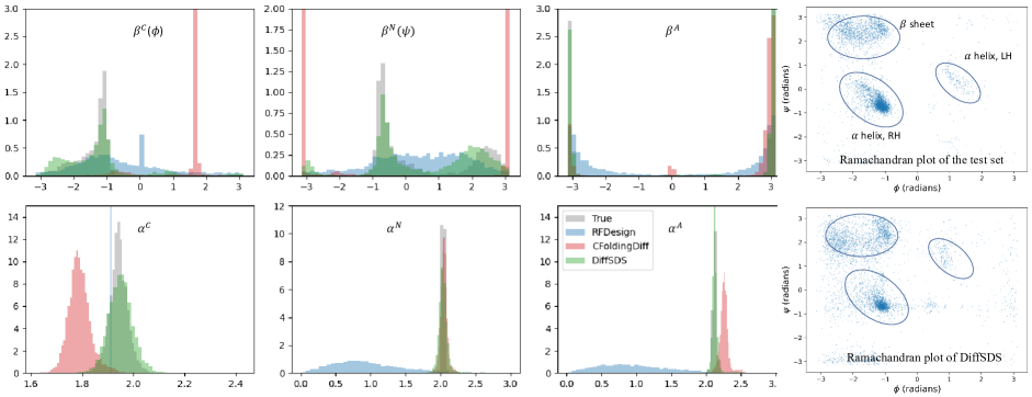
Figure 4: Angle distributions of various methods vs the test set distribution. DiffSDS produces the most similar angle distributions to those of the test set. Ramachandran plots also show that DiffSDS can produce realistic structural distributions

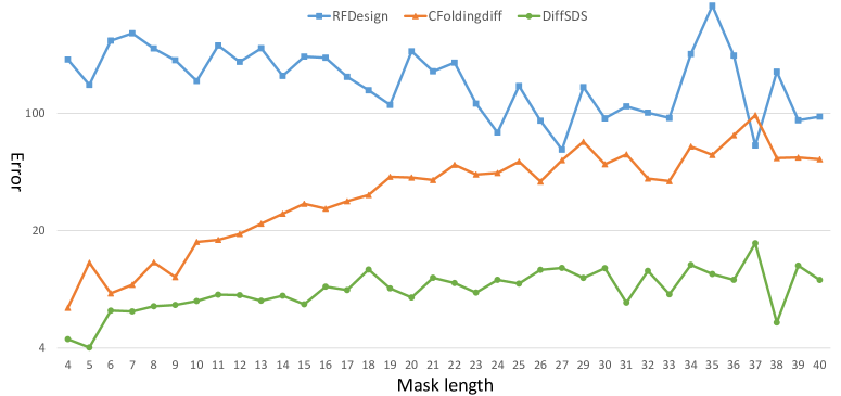
Figure 5: The connectivity error trend of different methods.

4.3 Connectivity

Objective & Setting

Do the designed structures connect the endpoints without breakage? As shown in Figure.1, the connectivity is an important indicator for the inpainting task, as disconnected proteins must be structurally abnormal. However, this metric has lacked attention in previous work, and we begin by defining the connectivity error as:

$$\text{Error}=||\bm{p}^{A}_{s}-\bm{\hat{p}}^{A}_{s}||+||\bm{p}^{A}_{e}-\bm{\hat{p}}^{A}_{e}||$$ (14)

where $s$ and $e$ are indexes of the start and end points of the masked structure, $\bm{\hat{p}}^{A}$ and $\bm{p}^{A}$ indicate the predicted and ground truth positions of the $C_{\alpha}$-carbon. Ideally, $\text{Error}=0$ means that endpoints are connected as expected.

Results & Analysis

From Table.2, we conclude that DiffSDS could achieve the lowest connectivity error compared to RFDesign and FoldingDiff, suggesting that it can better connect masked endpoints. We further show the trend of connectivity error with increasing mask length in Figure.5, from which we find that RFDesign performs poorly at all mask lengths, FoldingDiff’s connectivity error increases with mask length, while DiffSDS performs steadily and consistently better than all baselines.

	connectivity error
mask length	$<$10	10-15	$>$15
RFDesign	218.36	146.24	159.17
FoldingDiff	14.77	42.65	59.08
DiffSDS	6.93	9.93	10.61

Table 2: connectivity error of different methods.

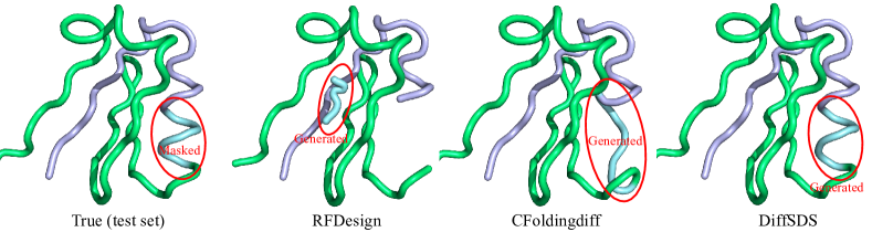
Figure 6: A protein inpating example. DiffSDS generates the most similar structure to the reference protein.

4.4 Non-overlapping

Objective & Setting

Will the designed structures be overlapped with existing backbones? We evaluate the spatial interaction between the generated structure ($\hat{\mathcal{M}}$) and the unmasked structure ($\mathcal{U}$), and define the interaction score as

$$\text{Score}_{d}=\sum_{i\in\hat{\mathcal{M}},j\in\mathcal{U}}\mathds{1}(||\bm{\hat{x}}_{i}-\bm{\hat{x}}_{j}||<d)$$ (15)

where $\mathds{1}(\cdot)$ is an indicator function. $\text{Score}_{d}$ records the number of pairwise interactions between masked and non-masked amino acids, with distances threshold $d$ $\mathring{A}$.

	$d=1\mathring{A}$			$d=3\mathring{A}$
mask length	$<$15	15-30	$>$30	$<$15	15-30	$>$30
True	266	345	139	268	406	139
RFDesign	280	357	153	861	1362	593
Foldingdiff	276	352	145	552	640	222
DiffSDS	270	356	141	472	632	178

Table 3: The number of spatial interactions.

Results & Analysis

As shown in Table.3, the spatial interactions of DiffSDS’s generated structures are closer to the test set than the baselines. This verifies that the non-overlap loss we introduced can avoid spatial overlap.

4.5 Ablation study

Objective&Setting

We conduct ablation experiments to investigate the impact of conditions and constraints on protein backbone inpainting. Specifically, we show how these factors affect the validation losses, including angle loss, length loss, and overlapping loss.

Results & Analysis

Limited to the page, we show the ablation details in the Appendix. As shown in Fig.7 and Fig.8, we find that: (1) the length condition and the sequence condition contribute to the reduction of $\mathcal{L}_{len}$ and $\mathcal{L}_{sim}$, respectively. This phenomenon suggests that the model can learn to generate structures with a predetermined length and that residue types can facilitate learning backbone angles. (2) Explicitly imposing geometric constraints on the model is necessary. If the constraints are removed, the $\mathcal{L}_{len}$ loss is difficult to reduce, and the $\mathcal{L}_{overlap}$ even increases, indicating the model could not generate geometrically reasonable structures. Fortunately, all these drawbacks could be eliminated by imposing geometric loss on the introduced direction space.

4.6 Designability

Objective & Setting

How likely are the generated proteins to be synthesized in the laboratory? We further measure the designability of the generated protein by the self-consistency TM score (scTM), which is first introduced by FoldingDiff. The generated backbones are fed into ESM-IF to obtain candidate protein sequences, which are subsequently folded into 3D structures by OmegaFold. scTM is the TM score between the newly folded structure and the original generated structure. If scTM$>0.5$, the corresponding generated backbone is considered designable.

Results & Analysis

As shown in Table4, the designability order is: DiffSDS$>$CFoldingDiff$>$RFDesign. On the full test set, DiffSDS generate 231 designable backbones, outperforming CFoldingDiff’s 217 and RFDesign’s 178. For proteins of more than 70 residues, the relative improvement is 8.6%; for long proteins of more than 70 residues, the relative improvement achieves 10%. Besides, DiffSDS outperforms previous methods in both average and median scTM scores. In Fig.6, we show a protein inpainting example, comparing different methods.

	scTM$>$0.5			scTM
	All	len$\leq$70	len$>$70	Mean	Median
RFDesign	178/378	65/148	113/230	0.51	0.48
CFoldingDiff	217/378	81/148	130/230	0.54	0.53
DiffSDS	231/378	88/148	143/230	0.56	0.55
Improvement	6.5%	8.6%	10%	3.7%	3.8%

Table 4: Designability of different methods.

5 Conclusion

This paper introduces and inserts a direction-based representation space on the language model to support efficient geometric feature computation and maintain modeling simplicity. By imposing geometric constraints on the direction space and applying the model during conditional diffusion, the proposed DiffSDS achieves significant improvements in protein backbone inpainting compared to baselines.

Appendix A Appendix

A.1 Related works

3D Molecule Generation

Generating 3D molecules to explore the local minima of the energy function (Conformation Generation) (Gebauer et al., 2019; Simm et al., 2020b, a; Shi et al., 2021; Xu et al., 2021; Luo et al., 2021; Xu et al., 2020; Ganea et al., 2021a; Xu et al., 2022; Hoogeboom et al., 2022; Jing et al., 2022; Zhu et al., 2022) or discover potential drug molecules binding to targeted proteins (3D Drug Design) (Imrie et al., 2020; Nesterov et al., 2020; Luo et al., 2022; Ragoza et al., 2022; Wu et al., 2022b; Huang et al., 2022a; Peng et al., 2022; Huang et al., 2022b; Wang et al., 2022b; Liu et al., 2022b) have attracted extensive attention in recent years. Compared to conformation generation that aims to predict the set of favourable conformers from the molecular graph, 3D Drug Design is more challenging in two aspects: (1) both conformation and molecule graph need to be generated, and (2) the generated molecules should satisfy multiple constraints, such as physical prior and protein-ligand binding affinity. We summarized representive works of 3D drug design in Table.5 in the appendix, where all the methods focus on small molecule design.

Table 5: 3D molecule generation models.

Method	Input	Github
Molecule Conformation Generation
G-SchNet (Gebauer et al., 2019)	–	PyTorch
CVGAE (Mansimov et al., 2019)	2D-graph	TF
GraphDG (Simm et al., 2020b)	2D-graph	PyTorch
MolGym (Simm et al., 2020a)	–	PyTorch
ConfGF (Shi et al., 2021)	2D-graph	PyTorch
ConfVAE (Xu et al., 2021)	2D-graph	PyTorch
DGSM (Luo et al., 2021)	2D-graph	–
CGCF (Xu et al., 2020)	2D-graph	PyTorch
GeoMol (Ganea et al., 2021a)	2D-graph	PyTorch
G-SphereNet (Luo & Ji, 2021)	–	PyTorch
GeoDiff (Xu et al., 2022)	2D-graph	PyTorch
EDM (Hoogeboom et al., 2022)	2D-graph	PyTorch
TorsionDiff (Jing et al., 2022)	2D-graph	PyTorch
DMCG (Zhu et al., 2022)	2D-graph	PyTorch
De novo Molecule Design
DeLinker (Imrie et al., 2020)	Protein Pocket 3D-fragments	TF
3DMolNet (Nesterov et al., 2020)	3D-geometry	–
cG-SchNet (Gebauer et al., 2022)	3D-geometry	PyTorch
Luo’s model (Luo et al., 2022)	Protein Pocket	PyTorch
LiGAN (Ragoza et al., 2022)	Protein Pocket	PyTorch
Bridge (Wu et al., 2022b)	Physical prior	–
MDM (Huang et al., 2022a)	2D-graph Properties	–
Pocket2Mol (Peng et al., 2022)	Protein Pocket	PyTorch
3DLinkcer (Huang et al., 2022b)	3D-fragments	PyTorch
CGVAE (Wang et al., 2022b)	Coarse Topology	PyTorch
GraphBP (Liu et al., 2022b)	Protein Pocket	PyTorch

Protein Design

In addition to small molecules, biomolecules such as proteins have also attracted considerable attention by researchers (Ding et al., 2022; Ovchinnikov & Huang, 2021; Gao et al., 2020; Strokach & Kim, 2022). We divide the mainstream protein design methods into three categories: protein sequence design (Li et al., 2014; Wu et al., 2021; Pearce & Zhang, 2021; Ingraham et al., 2019; Jing et al., 2020; Tan et al., 2022; Gao et al., 2022a; Hsu et al., 2022; Dauparas et al., 2022; Gao et al., 2022b; O’Connell et al., 2018; Wang et al., 2018; Qi & Zhang, 2020; Strokach et al., 2020; Chen et al., 2019; Zhang et al., 2020; Anand & Achim, 2022), unconditional protein structure generation (Anand & Huang, 2018; Sabban & Markovsky, 2020; Eguchi et al., 2022; Wu et al., 2022a), and conditional protein design (Lee & Kim, 2022; Wang et al., 2022a; Trippe et al., 2022; Lai et al., 2022; Fu & Sun, 2022; Tischer et al., 2020; Anand & Achim, 2022; Luo et al., ). Protein sequence design aims to discover protein sequences folding into the desired structure, and unconditional protein structure generation focus on generating new protein structures from noisy inputs. We are interested in conditional protein design and consider multiple constraints on the designed protein. For example, Wang’s model (Wang et al., 2022a), SMCDiff (Trippe et al., 2022) and Tischer’s model (Tischer et al., 2020) design the scaffold for the specified functional sites. ProteinSGM (Lee & Kim, 2022) mask short spans ($<8$ residues) of different secondary structures in different structures and treats the design task as a inpainting problem. CoordVAE (Lai et al., 2022) produces novel protein structures conditioned on the backbone template. RefineGNN (Jin et al., 2021), CEM (Fu & Sun, 2022), and DiffAb (Luo et al., ) aim to generate the complementarity-determining regions of the antibody. We summarized protein design model in Table.6.

Table 6: Protein Design Models.

Method	Input	Github
Unconditional protein structure generation
Anand’s model (Anand & Huang, 2018)	Noise	PyTorch
RamaNet (Sabban & Markovsky, 2020)	Noise	TF
Ig-VAE (Eguchi et al., 2022)	Noise	PyTorch
FoldingDiff (Wu et al., 2022a)	Noise	PyTorch
Protein seqeunce design
GraphTrans (Ingraham et al., 2019)	3D Backbone	PyTorch
GVP (Jing et al., 2020)	3D Backbone	PyTorch
GCA (Tan et al., 2022)	3D Backbone	PyTorch
AlphaDesign (Gao et al., 2022a)	3D Backbone	PyTorch
ESM-IF (Hsu et al., 2022)	3D Backbone	PyTorch
ProteinMPNN (Dauparas et al., 2022)	3D Backbone	PyTorch
PiFold (Gao et al., 2022b)	3D Backbone	PyTorch
Conditional protein design
ProteinSGM (Lee & Kim, 2022)	Masked structures	–
Wang’s model (Wang et al., 2022a)	Functional sites	PyTorch
SMCDiff (Trippe et al., 2022)	Functional motifs	–
CoordVAE (Lai et al., 2022)	Backbone Template	–
CEM (Fu & Sun, 2022)	CDR geometry	–
Tischer’s model (Tischer et al., 2020)	Functional motifs	TF
Anand’s model (Anand & Achim, 2022)	Multiple conditions	–
RefineGNN (Jin et al., 2021)	Antigen structure	PyTorch
DiffAb (Luo et al., )	Antigen structure	PyTorch

A.2 Algorithms

Algorithm 1 $\text{place}(\bm{x},\alpha,\beta,\bm{d}_{1},\bm{d}_{2},r)$

1:  Input: $\bm{x},\alpha,\beta,\bm{d}_{1},\bm{d}_{2}$

2:  $\bm{\tilde{d}}=[-\cos{\alpha},\cos{\beta}\sin{\alpha},\sin{\beta}\sin{\alpha}]^{T}$

3:  $R=[\bm{d}_{1},(\bm{d}_{2}\times\bm{d}_{1})\times\bm{d}_{1},\bm{d}_{2}\times\bm{d}_{1}]$

4:  $\bm{d}=R\bm{\tilde{d}}$

5:  Return: $\bm{x}+r\bm{d}$

Algorithm 2 $\text{dihedral}(\bm{v}_{1},\bm{v}_{2},\bm{v}_{3})$

1:  Input: $\bm{v}_{1},\bm{v}_{2},\bm{v}_{3}$

2:  $\bm{n}_{1}=\bm{v}_{1}\times\bm{v}_{2}$

3:  $\bm{n}_{2}=\bm{v}_{2}\times\bm{v}_{3}$

4:  $x=(\bm{n}_{1})^{T}\bm{n}_{2}$

5:  $y=\bm{n}_{1}\times\bm{n}_{2}$

6:  Return: $\arctan{\frac{y}{x}}$

A.3 Diffusion

Forward process

We start from the standard diffusion process $x_{0}\rightarrow x_{1}\rightarrow\cdots\rightarrow x_{T}$, where the forward translation kernel from timestamp $s$ to $t$ is defined as $q(x_{t}|x_{s})=\mathcal{N}(x_{t};\alpha_{t|s}x_{s},\sigma_{t|s}^{2}I)$, $s\leq t$. Denote $\alpha_{t}=\alpha_{t|0},\sigma_{t}=\sigma_{t|0}$, and $q(x_{0}|x_{0})=\mathcal{N}(x_{0};\alpha_{0}x,\sigma_{0}^{2}I),\alpha_{0}=1,\sigma_{0}=0$. We will show that $\alpha_{t|s}=\alpha_{t}/\alpha_{s},\sigma^{2}_{t|s}=\sigma^{2}_{t}-\alpha^{2}_{t|s}\sigma^{2}_{s}$.

Proof.

$$q(x_{t}|x_{s})= \mathcal{N}(x_{t};\alpha_{t|s}x_{s},\sigma_{t|s}^{2}I)$$ (16)

$$\Rightarrow x_{t}= \alpha_{t|t-1}x_{t-1}+\sigma_{t|t-1}\epsilon_{t-1} {\color[rgb]{.5,.5,.5}x_{t}\sim q(x_{t}|x_{t-1})}$$

$$= \alpha_{t|t-1}(\alpha_{t-1|s}x_{s}+\sigma_{t-1|s}\epsilon_{s})+\sigma_{t|t-1}\epsilon_{t-1} {\color[rgb]{.5,.5,.5}x_{t-1}\sim q(x_{t-1}|x_{s})}$$

$$= \alpha_{t|t-1}\alpha_{t-1|s}x_{s}+\alpha_{t|t-1}\sigma_{t-1|s}\epsilon_{s}+\sigma_{t|t-1}\epsilon_{t-1}$$

$$= (\alpha_{t|t-1}\alpha_{t-1|s})x_{s}+\sqrt{\alpha^{2}_{t|t-1}\sigma^{2}_{t-1|s}+\sigma^{2}_{t|t-1}}\hat{\epsilon}_{s}$$

$$= \alpha_{t|s}x_{s}+\sigma_{t|s}\epsilon_{s} {\color[rgb]{.5,.5,.5}x_{t}\sim q(x_{t}|x_{s})}$$

We conclude that $\alpha_{t|s}=\alpha_{t|t-1}\alpha_{t-1|s}$ and $\sigma_{t|s}=\sqrt{\alpha^{2}_{t|t-1}\sigma^{2}_{t-1|s}+\sigma^{2}_{t|t-1}}$.

For $\alpha_{t|s}=\alpha_{t|t-1}\alpha_{t-1|s}$,

$$\alpha_{t|s} =\alpha_{t|t-1}\alpha_{t-1|s}$$ (17)

$$=\alpha_{t|t-1}\alpha_{t-1|t-2}\alpha_{t-2|s}$$

$$\cdots$$

$$=\prod_{i=s+1}^{t}\alpha_{i|i-1}$$

$$=\prod_{i=s+1}^{t}\frac{\alpha_{i}}{\alpha_{i-1}}$$

For $\sigma_{t|s}=\sqrt{\alpha^{2}_{t|t-1}\sigma^{2}_{t-1|s}+\sigma^{2}_{t|t-1}}$, let $s=0$, then $\sigma^{2}_{t|t-1}=\sigma^{2}_{t}-\alpha^{2}_{t|t-1}\sigma^{2}_{t-1}$. Therefore,

$$\sigma^{2}_{t|s} =\alpha^{2}_{t|t-1}\sigma^{2}_{t-1|s}+\sigma^{2}_{t|t-1}$$ (18)

$$=\alpha^{2}_{t|t-1}(\alpha^{2}_{t-1|t-2}\sigma^{2}_{t-2|s}+\sigma^{2}_{t-1|t-2})+\sigma^{2}_{t|t-1}$$

$$=\alpha^{2}_{t|t-1}\alpha^{2}_{t-1|t-2}\sigma^{2}_{t-2|s}+\alpha^{2}_{t|t-1}\sigma^{2}_{t-1|t-2}+\sigma^{2}_{t|t-1}$$

$$=\alpha^{2}_{t|t-2}\sigma^{2}_{t-2|s}+\alpha^{2}_{t|t-1}\sigma^{2}_{t-1|t-2}+\alpha^{2}_{t|t}\sigma^{2}_{t|t-1}$$

$$=\sum_{k=s+1}^{t}{\alpha^{2}_{t|k}\sigma^{2}_{k|k-1}}$$

$$=\sum_{k=s+1}^{t}{\alpha^{2}_{t|k}(\sigma_{k}^{2}-\alpha^{2}_{k|k-1}\sigma^{2}_{k-1})} {\color[rgb]{.5,.5,.5}\text{Apply }\sigma^{2}_{t|t-1}=\sigma^{2}_{t}-\alpha^{2}_{t|t-1}\sigma^{2}_{t-1}}$$

$$=\sum_{k=s+1}^{t}{\alpha^{2}_{t|k}\sigma_{k}^{2}}-\sum_{k=s+1}^{t}{\alpha^{2}_{t|k-1}\sigma_{k-1}^{2}}$$

$$=\alpha^{2}_{t|t}\sigma_{t}^{2}-\alpha^{2}_{t|s}\sigma_{s}^{2}$$

$$=\sigma_{t}^{2}-\alpha^{2}_{t|s}\sigma_{s}^{2}$$

∎

Reverse process

As to the backward process $x_{T}\rightarrow x_{T-1}\rightarrow\cdots\rightarrow x_{0}$, the neural network aims to maximize $q(x_{s}|x_{t},x_{0})=\mathcal{N}(z_{s};\hat{\mu}_{s},\hat{\sigma}_{s}^{2}I)$, where

$$\begin{cases}\hat{\sigma}_{s}=\frac{\sigma_{t|s}\sigma_{s}}{\sigma_{t}}\\ \hat{\mu}_{s}=\frac{1}{\alpha_{t|s}}x_{t}-\frac{\alpha_{t|s}}{\sigma_{t}}\epsilon_{t}\end{cases}$$ (19)

Proof.

Recall that $\mathcal{N}(z;\mu,\sigma I)\propto\exp{\left(-\frac{||z-\mu||^{2}}{2\sigma^{2}}\right)}$, the backward translation could be derived by Bayes’ Theorem:

$$q(x_{s}|x_{t},x_{0}) =\frac{q(x_{t}|x_{s})q(x_{s}|x_{0})}{q(x_{t}|x_{0})}$$ (20)

$$\propto\exp{\left[-\frac{1}{2}\left(\frac{||x_{t}-\alpha_{t|s}x_{s}||^{2}}{\sigma_{t|s}^{2}}+\frac{||x_{s}-\alpha_{s}x_{0}||^{2}}{\sigma_{s}^{2}}-\frac{||x_{t}-\alpha_{t}x_{0}||^{2}}{\sigma_{t}^{2}}\right)\right]}$$

from which we can derive $q(z_{s}|z_{t},x_{0})=\mathcal{N}(z_{s};\hat{\mu}_{s},\hat{\sigma}_{s}^{2}I)$, and

$$\begin{cases}\frac{1}{\hat{\sigma}_{s}^{2}}=\frac{\alpha_{t|s}^{2}}{\sigma_{t|s}^{2}}+\frac{1}{\sigma_{s}^{2}}\\ -2\frac{\hat{\mu}_{s}}{\hat{\sigma}_{s}^{2}}=-2\frac{x_{t}\alpha_{t|s}}{\sigma_{t|s}^{2}}-2\frac{\alpha_{s}x_{0}}{\sigma_{s}^{2}}\end{cases}$$ (21)

finally

$$\begin{cases}\hat{\sigma}_{s}=\frac{\sigma_{t|s}\sigma_{s}}{\sigma_{t}}\\ \hat{\mu}_{s}=\frac{1}{\alpha_{t|s}}x_{t}-\frac{\alpha_{s|t}\sigma^{2}_{t|s}}{\sigma_{t}}\epsilon_{t}\end{cases}$$ (22)

Note that

$$-2\frac{\hat{\mu}_{s}}{\hat{\sigma}_{s}^{2}}= -2\frac{(x_{t})\alpha_{t|s}}{\sigma_{t|s}^{2}}-2\frac{(\alpha_{s}x_{0})}{\sigma_{s}^{2}}$$ (23)

$$\hat{\mu}_{s}= \frac{(x_{t})\alpha_{t|s}}{\sigma_{t|s}^{2}}(\frac{\sigma_{t|s}\sigma_{s}}{\sigma_{t}})^{2}+\frac{(\alpha_{s}x_{0})}{\sigma_{s}^{2}}(\frac{\sigma_{t|s}\sigma_{s}}{\sigma_{t}})^{2}$$

$$\hat{\mu}_{s}= \frac{(x_{t})\alpha_{t|s}\sigma_{s}^{2}}{\sigma_{t}^{2}}+\frac{(\alpha_{s}x_{0})\sigma_{t|s}^{2}}{\sigma_{t}^{2}}$$

$$\hat{\mu}_{s}= \frac{(x_{t})\alpha_{t|s}\sigma_{s}^{2}}{\sigma_{t}^{2}}+\alpha_{s}\frac{x_{t}-\sigma_{t}\epsilon_{t}}{\alpha_{t}}\frac{\sigma_{t|s}^{2}}{\sigma_{t}^{2}}$$

$$\hat{\mu}_{s}= (\frac{\alpha_{t|s}\sigma_{s}^{2}}{\sigma_{t}^{2}}+\frac{\alpha_{s}\sigma_{t|s}^{2}}{\alpha_{t}\sigma_{t}^{2}})x_{t}-\frac{\alpha_{s}\sigma_{t|s}^{2}}{\alpha_{t}\sigma_{t}}\epsilon_{t}$$

$$\hat{\mu}_{s}= \frac{1}{\alpha_{t|s}}x_{t}-\frac{\alpha_{s|t}\sigma^{2}_{t|s}}{\sigma_{t}}\epsilon_{t}$$

∎

A.4 Ablation

Objective&Setting

We conduct ablation experiments to investigate the impact of conditions and constraints on protein backbone inpainting. Specifically, we show how these factors affect the validation losses, including angle loss, length loss, and overlapping loss.

Results & Analysis

As shown in Fig.7 and Fig.8, we find that: (1) the length condition and the sequence condition contribute to the reduction of $\mathcal{L}_{len}$ and $\mathcal{L}_{sim}$, respectively. This phenomenon suggests that the model can learn to generate structures with a predetermined length and that residue types can facilitate learning backbone angles. (2) Explicitly imposing geometric constraints on the model is necessary. If the constraints are removed, the $\mathcal{L}_{len}$ loss is difficult to reduce, and the $\mathcal{L}_{overlap}$ even increases, indicating the model could not generate geometrically reasonable structures. Fortunately, all these drawbacks could be eliminated by imposing geometric loss on the introduced direction space.

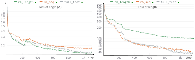
Figure 7: Ablation of conditions. We remove length condition or residue type embedding from the baseline ($\text{full}\_{\text{feat}}$) model, resulting in $\text{rm}\_{\text{length}}$ and $\text{rm}\_{\text{seq}}$, respectively. We show the loss curves for angle ($\phi$) and length on the validation set, revealing the effect of the conditions.

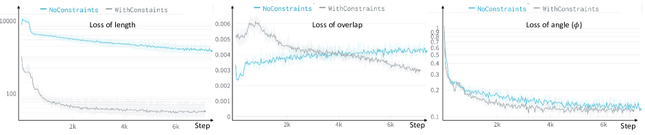
Figure 8: Ablation of constraints. We show the validation loss curves in the constrained and unconstrained cases. The unconstrained case means that $mathcal{L}_{len}$ and $mathcal{L}_{overlap}$ are not imposed on the model during training.

References

- Anand & Achim (2022) Anand, N. and Achim, T. Protein structure and sequence generation with equivariant denoising diffusion probabilistic models. arXiv preprint arXiv:2205.15019, 2022.
- Anand & Huang (2018) Anand, N. and Huang, P. Generative modeling for protein structures. Advances in neural information processing systems, 31, 2018.
- Austin et al. (2021) Austin, J., Johnson, D. D., Ho, J., Tarlow, D., and van den Berg, R. Structured denoising diffusion models in discrete state-spaces. Advances in Neural Information Processing Systems, 34:17981–17993, 2021.
- Baranchuk et al. (2021) Baranchuk, D., Rubachev, I., Voynov, A., Khrulkov, V., and Babenko, A. Label-efficient semantic segmentation with diffusion models. arXiv preprint arXiv:2112.03126, 2021.
- Cao et al. (2022) Cao, H., Tan, C., Gao, Z., Chen, G., Heng, P.-A., and Li, S. Z. A survey on generative diffusion model. arXiv preprint arXiv:2209.02646, 2022.
- Chen et al. (2020) Chen, N., Zhang, Y., Zen, H., Weiss, R. J., Norouzi, M., and Chan, W. Wavegrad: Estimating gradients for waveform generation. arXiv preprint arXiv:2009.00713, 2020.
- Chen et al. (2019) Chen, S., Sun, Z., Lin, L., Liu, Z., Liu, X., Chong, Y., Lu, Y., Zhao, H., and Yang, Y. To improve protein sequence profile prediction through image captioning on pairwise residue distance map. Journal of chemical information and modeling, 60(1):391–399, 2019.
- Chen et al. (2022) Chen, T., Zhang, R., and Hinton, G. Analog bits: Generating discrete data using diffusion models with self-conditioning. arXiv preprint arXiv:2208.04202, 2022.
- Dauparas et al. (2022) Dauparas, J., Anishchenko, I., Bennett, N., Bai, H., Ragotte, R. J., Milles, L. F., Wicky, B. I., Courbet, A., de Haas, R. J., Bethel, N., et al. Robust deep learning based protein sequence design using proteinmpnn. bioRxiv, 2022.
- Ding et al. (2022) Ding, W., Nakai, K., and Gong, H. Protein design via deep learning. Briefings in bioinformatics, 23(3):bbac102, 2022.
- Drake & Pettitt (2020) Drake, J. A. and Pettitt, B. M. Physical chemistry of the protein backbone: Enabling the mechanisms of intrinsic protein disorder. The Journal of Physical Chemistry B, 124(22):4379–4390, 2020.
- Eguchi et al. (2022) Eguchi, R. R., Choe, C. A., and Huang, P.-S. Ig-vae: Generative modeling of protein structure by direct 3d coordinate generation. Biorxiv, pp. 2020–08, 2022.
- Ferruz et al. (2022) Ferruz, N., Heinzinger, M., Akdel, M., Goncearenco, A., Naef, L., and Dallago, C. From sequence to function through structure: deep learning for protein design. Computational and Structural Biotechnology Journal, 2022.
- Fu & Sun (2022) Fu, T. and Sun, J. Antibody complementarity determining regions (cdrs) design using constrained energy model. In Proceedings of the 28th ACM SIGKDD Conference on Knowledge Discovery and Data Mining, pp. 389–399, 2022.
- Ganea et al. (2021a) Ganea, O., Pattanaik, L., Coley, C., Barzilay, R., Jensen, K., Green, W., and Jaakkola, T. Geomol: Torsional geometric generation of molecular 3d conformer ensembles. Advances in Neural Information Processing Systems, 34:13757–13769, 2021a.
- Ganea et al. (2021b) Ganea, O.-E., Huang, X., Bunne, C., Bian, Y., Barzilay, R., Jaakkola, T., and Krause, A. Independent se (3)-equivariant models for end-to-end rigid protein docking. arXiv preprint arXiv:2111.07786, 2021b.
- Gao et al. (2020) Gao, W., Mahajan, S. P., Sulam, J., and Gray, J. J. Deep learning in protein structural modeling and design. Patterns, 1(9):100142, 2020.
- Gao et al. (2022a) Gao, Z., Tan, C., Li, S., et al. Alphadesign: A graph protein design method and benchmark on alphafolddb. arXiv preprint arXiv:2202.01079, 2022a.
- Gao et al. (2022b) Gao, Z., Tan, C., and Li, S. Z. Pifold: Toward effective and efficient protein inverse folding. arXiv preprint arXiv:2209.12643, 2022b.
- Gebauer et al. (2019) Gebauer, N., Gastegger, M., and Schütt, K. Symmetry-adapted generation of 3d point sets for the targeted discovery of molecules. Advances in neural information processing systems, 32, 2019.
- Gebauer et al. (2022) Gebauer, N. W., Gastegger, M., Hessmann, S. S., Müller, K.-R., and Schütt, K. T. Inverse design of 3d molecular structures with conditional generative neural networks. Nature communications, 13(1):1–11, 2022.
- Ho et al. (2020) Ho, J., Jain, A., and Abbeel, P. Denoising diffusion probabilistic models. Advances in Neural Information Processing Systems, 33:6840–6851, 2020.
- Hoogeboom et al. (2022) Hoogeboom, E., Satorras, V. G., Vignac, C., and Welling, M. Equivariant diffusion for molecule generation in 3d. In International Conference on Machine Learning, pp. 8867–8887. PMLR, 2022.
- Hsu et al. (2022) Hsu, C., Verkuil, R., Liu, J., Lin, Z., Hie, B., Sercu, T., Lerer, A., and Rives, A. Learning inverse folding from millions of predicted structures. bioRxiv, 2022.
- Huang et al. (2022a) Huang, L., Zhang, H., Xu, T., and Wong, K.-C. Mdm: Molecular diffusion model for 3d molecule generation. arXiv preprint arXiv:2209.05710, 2022a.
- Huang et al. (2022b) Huang, Y., Peng, X., Ma, J., and Zhang, M. 3dlinker: An e (3) equivariant variational autoencoder for molecular linker design. arXiv preprint arXiv:2205.07309, 2022b.
- Imrie et al. (2020) Imrie, F., Bradley, A. R., van der Schaar, M., and Deane, C. M. Deep generative models for 3d linker design. Journal of chemical information and modeling, 60(4):1983–1995, 2020.
- Ingraham et al. (2019) Ingraham, J., Garg, V. K., Barzilay, R., and Jaakkola, T. Generative models for graph-based protein design. 2019.
- Jin et al. (2021) Jin, W., Wohlwend, J., Barzilay, R., and Jaakkola, T. Iterative refinement graph neural network for antibody sequence-structure co-design. arXiv preprint arXiv:2110.04624, 2021.
- Jing et al. (2020) Jing, B., Eismann, S., Suriana, P., Townshend, R. J., and Dror, R. Learning from protein structure with geometric vector perceptrons. arXiv preprint arXiv:2009.01411, 2020.
- Jing et al. (2022) Jing, B., Corso, G., Chang, J., Barzilay, R., and Jaakkola, T. Torsional diffusion for molecular conformer generation. arXiv preprint arXiv:2206.01729, 2022.
- Jumper et al. (2021) Jumper, J., Evans, R., Pritzel, A., Green, T., Figurnov, M., Ronneberger, O., Tunyasuvunakool, K., Bates, R., Žídek, A., Potapenko, A., et al. Highly accurate protein structure prediction with alphafold. Nature, 596(7873):583–589, 2021.
- Kong et al. (2020) Kong, Z., Ping, W., Huang, J., Zhao, K., and Catanzaro, B. Diffwave: A versatile diffusion model for audio synthesis. arXiv preprint arXiv:2009.09761, 2020.
- Lai et al. (2022) Lai, B., Xu, J., et al. End-to-end deep structure generative model for protein design. bioRxiv, 2022.
- Lee & Han (2021) Lee, J. and Han, S. Nu-wave: A diffusion probabilistic model for neural audio upsampling. arXiv preprint arXiv:2104.02321, 2021.
- Lee & Kim (2022) Lee, J. S. and Kim, P. M. Proteinsgm: Score-based generative modeling for de novo protein design. bioRxiv, 2022.
- Li et al. (2022) Li, X. L., Thickstun, J., Gulrajani, I., Liang, P., and Hashimoto, T. B. Diffusion-lm improves controllable text generation. arXiv preprint arXiv:2205.14217, 2022.
- Li et al. (2014) Li, Z., Yang, Y., Faraggi, E., Zhan, J., and Zhou, Y. Direct prediction of profiles of sequences compatible with a protein structure by neural networks with fragment-based local and energy-based nonlocal profiles. Proteins: Structure, Function, and Bioinformatics, 82(10):2565–2573, 2014.
- Liu et al. (2022a) Liu, J., Li, C., Ren, Y., Chen, F., and Zhao, Z. Diffsinger: Singing voice synthesis via shallow diffusion mechanism. In Proceedings of the AAAI Conference on Artificial Intelligence, volume 36, pp. 11020–11028, 2022a.
- Liu et al. (2022b) Liu, M., Luo, Y., Uchino, K., Maruhashi, K., and Ji, S. Generating 3d molecules for target protein binding. arXiv preprint arXiv:2204.09410, 2022b.
- Lugmayr et al. (2022) Lugmayr, A., Danelljan, M., Romero, A., Yu, F., Timofte, R., and Van Gool, L. Repaint: Inpainting using denoising diffusion probabilistic models. In Proceedings of the IEEE/CVF Conference on Computer Vision and Pattern Recognition, pp. 11461–11471, 2022.
- (42) Luo, S., Su, Y., Peng, X., Wang, S., Peng, J., and Ma, J. Antigen-specific antibody design and optimization with diffusion-based generative models for protein structures.
- Luo et al. (2021) Luo, S., Shi, C., Xu, M., and Tang, J. Predicting molecular conformation via dynamic graph score matching. Advances in Neural Information Processing Systems, 34:19784–19795, 2021.
- Luo et al. (2022) Luo, S., Guan, J., Ma, J., and Peng, J. A 3d molecule generative model for structure-based drug design. arXiv preprint arXiv:2203.10446, 2022.
- Luo & Ji (2021) Luo, Y. and Ji, S. An autoregressive flow model for 3d molecular geometry generation from scratch. In International Conference on Learning Representations, 2021.
- Mansimov et al. (2019) Mansimov, E., Mahmood, O., Kang, S., and Cho, K. Molecular geometry prediction using a deep generative graph neural network. Scientific reports, 9(1):1–13, 2019.
- Müller-Späth et al. (2010) Müller-Späth, S., Soranno, A., Hirschfeld, V., Hofmann, H., Rüegger, S., Reymond, L., Nettels, D., and Schuler, B. Charge interactions can dominate the dimensions of intrinsically disordered proteins. Proceedings of the National Academy of Sciences, 107(33):14609–14614, 2010.
- Nesterov et al. (2020) Nesterov, V., Wieser, M., and Roth, V. 3dmolnet: a generative network for molecular structures. arXiv preprint arXiv:2010.06477, 2020.
- O’Connell et al. (2018) O’Connell, J., Li, Z., Hanson, J., Heffernan, R., Lyons, J., Paliwal, K., Dehzangi, A., Yang, Y., and Zhou, Y. Spin2: Predicting sequence profiles from protein structures using deep neural networks. Proteins: Structure, Function, and Bioinformatics, 86(6):629–633, 2018.
- Ovchinnikov & Huang (2021) Ovchinnikov, S. and Huang, P.-S. Structure-based protein design with deep learning. Current opinion in chemical biology, 65:136–144, 2021.
- Pearce & Zhang (2021) Pearce, R. and Zhang, Y. Deep learning techniques have significantly impacted protein structure prediction and protein design. Current opinion in structural biology, 68:194–207, 2021.
- Peng et al. (2022) Peng, X., Luo, S., Guan, J., Xie, Q., Peng, J., and Ma, J. Pocket2mol: Efficient molecular sampling based on 3d protein pockets. arXiv preprint arXiv:2205.07249, 2022.
- Qi & Zhang (2020) Qi, Y. and Zhang, J. Z. Densecpd: improving the accuracy of neural-network-based computational protein sequence design with densenet. Journal of chemical information and modeling, 60(3):1245–1252, 2020.
- Ragoza et al. (2022) Ragoza, M., Masuda, T., and Koes, D. R. Generating 3D molecules conditional on receptor binding sites with deep generative models. Chem Sci, 13:2701–2713, Feb 2022. doi: 10.1039/D1SC05976A.
- Sabban & Markovsky (2020) Sabban, S. and Markovsky, M. Ramanet: Computational de novo helical protein backbone design using a long short-term memory generative neural network. bioRxiv, pp. 671552, 2020.
- Shi et al. (2021) Shi, C., Luo, S., Xu, M., and Tang, J. Learning gradient fields for molecular conformation generation. In International Conference on Machine Learning, pp. 9558–9568. PMLR, 2021.
- Simm et al. (2020a) Simm, G., Pinsler, R., and Hernández-Lobato, J. M. Reinforcement learning for molecular design guided by quantum mechanics. In International Conference on Machine Learning, pp. 8959–8969. PMLR, 2020a.
- Simm et al. (2020b) Simm, G. N. C., Hernández-Lobato, J. M., XXX, and XXX. A generative model for molecular distance geometry. In Proceedings of the 37th International Conference on Machine Learning, ICML’20. JMLR.org, 2020b.
- Sohl-Dickstein et al. (2015) Sohl-Dickstein, J., Weiss, E., Maheswaranathan, N., and Ganguli, S. Deep unsupervised learning using nonequilibrium thermodynamics. In International Conference on Machine Learning, pp. 2256–2265. PMLR, 2015.
- Song et al. (2020) Song, Y., Sohl-Dickstein, J., Kingma, D. P., Kumar, A., Ermon, S., and Poole, B. Score-based generative modeling through stochastic differential equations. arXiv preprint arXiv:2011.13456, 2020.
- Spassov et al. (2007) Spassov, V. Z., Yan, L., and Flook, P. K. The dominant role of side-chain backbone interactions in structural realization of amino acid code. chirotor: A side-chain prediction algorithm based on side-chain backbone interactions. Protein Science, 16(3):494–506, 2007.
- Strokach & Kim (2022) Strokach, A. and Kim, P. M. Deep generative modeling for protein design. Current opinion in structural biology, 72:226–236, 2022.
- Strokach et al. (2020) Strokach, A., Becerra, D., Corbi-Verge, C., Perez-Riba, A., and Kim, P. M. Fast and flexible protein design using deep graph neural networks. Cell Systems, 11(4):402–411, 2020.
- Tan et al. (2022) Tan, C., Gao, Z., Xia, J., and Li, S. Z. Generative de novo protein design with global context. arXiv preprint arXiv:2204.10673, 2022.
- Tischer et al. (2020) Tischer, D., Lisanza, S., Wang, J., Dong, R., Anishchenko, I., Milles, L. F., Ovchinnikov, S., and Baker, D. Design of proteins presenting discontinuous functional sites using deep learning. Biorxiv, 2020.
- Trippe et al. (2022) Trippe, B. L., Yim, J., Tischer, D., Broderick, T., Baker, D., Barzilay, R., and Jaakkola, T. Diffusion probabilistic modeling of protein backbones in 3d for the motif-scaffolding problem. arXiv preprint arXiv:2206.04119, 2022.
- Wang et al. (2018) Wang, J., Cao, H., Zhang, J. Z., and Qi, Y. Computational protein design with deep learning neural networks. Scientific reports, 8(1):1–9, 2018.
- Wang et al. (2022a) Wang, J., Lisanza, S., Juergens, D., Tischer, D., Watson, J. L., Castro, K. M., Ragotte, R., Saragovi, A., Milles, L. F., Baek, M., et al. Scaffolding protein functional sites using deep learning. Science, 377(6604):387–394, 2022a.
- Wang et al. (2022b) Wang, W., Xu, M., Cai, C., Miller, B. K., Smidt, T., Wang, Y., Tang, J., and Gómez-Bombarelli, R. Generative coarse-graining of molecular conformations. arXiv preprint arXiv:2201.12176, 2022b.
- Whang et al. (2022) Whang, J., Delbracio, M., Talebi, H., Saharia, C., Dimakis, A. G., and Milanfar, P. Deblurring via stochastic refinement. In Proceedings of the IEEE/CVF Conference on Computer Vision and Pattern Recognition, pp. 16293–16303, 2022.
- Wolleb et al. (2022) Wolleb, J., Sandkühler, R., Bieder, F., Valmaggia, P., and Cattin, P. C. Diffusion models for implicit image segmentation ensembles. In International Conference on Medical Imaging with Deep Learning, pp. 1336–1348. PMLR, 2022.
- Wu et al. (2022a) Wu, K. E., Yang, K. K., Berg, R. v. d., Zou, J. Y., Lu, A. X., and Amini, A. P. Protein structure generation via folding diffusion. arXiv preprint arXiv:2209.15611, 2022a.
- Wu et al. (2022b) Wu, L., Gong, C., Liu, X., Ye, M., and Liu, Q. Diffusion-based molecule generation with informative prior bridges. arXiv preprint arXiv:2209.00865, 2022b.
- Wu et al. (2021) Wu, Z., Johnston, K. E., Arnold, F. H., and Yang, K. K. Protein sequence design with deep generative models. Current opinion in chemical biology, 65:18–27, 2021.
- Xu et al. (2020) Xu, M., Luo, S., Bengio, Y., Peng, J., and Tang, J. Learning neural generative dynamics for molecular conformation generation. In International Conference on Learning Representations, 2020.
- Xu et al. (2021) Xu, M., Wang, W., Luo, S., Shi, C., Bengio, Y., Gomez-Bombarelli, R., and Tang, J. An end-to-end framework for molecular conformation generation via bilevel programming. In International Conference on Machine Learning, pp. 11537–11547. PMLR, 2021.
- Xu et al. (2022) Xu, M., Yu, L., Song, Y., Shi, C., Ermon, S., and Tang, J. Geodiff: A geometric diffusion model for molecular conformation generation. arXiv preprint arXiv:2203.02923, 2022.
- Zhang et al. (2020) Zhang, Y., Chen, Y., Wang, C., Lo, C.-C., Liu, X., Wu, W., and Zhang, J. Prodconn: Protein design using a convolutional neural network. Proteins: Structure, Function, and Bioinformatics, 88(7):819–829, 2020.
- Zhu et al. (2022) Zhu, J., Xia, Y., Liu, C., Wu, L., Xie, S., Wang, T., Wang, Y., Zhou, W., Qin, T., Li, H., et al. Direct molecular conformation generation. arXiv preprint arXiv:2202.01356, 2022.