Fully transformer-based biomarker prediction from colorectal cancer histology: a large-scale multicentric study

Abstract

Background: Deep learning (DL) can extract predictive and prognostic biomarkers from routine pathology slides in colorectal cancer. For example, a DL test for the diagnosis of microsatellite instability (MSI) in CRC has been approved in 2022. Current approaches rely on convolutional neural networks (CNNs). Transformer networks are outperforming CNNs and are replacing them in many applications, but have not been used for biomarker prediction in cancer at a large scale. In addition, most DL approaches have been trained on small patient cohorts, which limits their clinical utility.

Methods: In this study, we developed a new fully transformer-based pipeline for end-to-end biomarker prediction from pathology slides. We combine a pre-trained transformer encoder and a transformer network for patch aggregation, capable of yielding single and multi-target prediction at patient level. We train our pipeline on over 9,000 patients from 10 colorectal cancer cohorts.

Results: A fully transformer-based approach massively improves the performance, generalizability, data efficiency, and interpretability as compared with current state-of-the-art algorithms. After training on a large multicenter cohort, we achieve a sensitivity of 0.97 with a negative predictive value of 0.99 for MSI prediction on surgical resection specimens. We demonstrate for the first time that resection specimen-only training reaches clinical-grade performance on endoscopic biopsy tissue, solving a long-standing diagnostic problem.

Interpretation: A fully transformer-based end-to-end pipeline trained on thousands of pathology slides yields clinical-grade performance for biomarker prediction on surgical resections and biopsies. Our new methods are freely available under an open source license.

Keywords Weakly-supvervised learning  $\cdot$ Biomarker prediction  $\cdot$ Transformer

1 Introduction

Precision oncology in colorectal cancer (CRC) requires the evaluation of genetic biomarkers, such as microsatellite instability (MSI) (Kather et al., 2019; Cao et al., 2020; Echle et al., 2020; Bilal et al., 2021; Lee et al., 2021; Schirris et al., 2022; Schrammen et al., 2022; Yamashita et al., 2021) and mutations in the BRAF (Bilal et al., 2021; Schrammen et al., 2022) NRAS/KRAS (Jang et al., 2020) genes. These biomarkers are typically measured by polymerase chain reaction (PCR), sequencing (for BRAF and KRAS), or immunohistochemical assays. Biomarker identification in patients with CRC is an important step in providing treatment as recommended by various medical guidelines, such as those in the USA (NCCN guideline) (Benson et al., 2018), UK (NICE guideline) (NIC, ), and EU (ESMO guideline) (Schmoll et al., 2012). Increasingly, genetic biomarkers such as MSI are also used in earlier tumor stages of CRC (Chalabi et al., 2022). In the future, the importance of biomarker-stratified therapy will likely increase (Vacante et al., 2018). The presence of MSI should also trigger additional diagnostic processes for Lynch syndrome, one of the most prevalent hereditary cancer syndromes. However, genetic diagnostic assays have several disadvantages. For many patients in low- and middle-income countries, genetic biomarkers are not routinely available due to the prohibitive costs and complex infrastructure required for testing. Even in high-income countries with universal healthcare coverage where genetic biomarkers may be routinely available, their utilization is not without its drawbacks. In such contexts, biomarker assessment can take several days to weeks delaying therapy decisions (Lim et al., 2015).

The diagnosis of CRC requires a pathologist’s histopathological evaluation of tissue sections. Thus, tissue sections stained with hematoxylin and eosin (H&E) are routinely available for all patients with CRC. Since 2019, dozens of studies have shown that Deep Learning (DL) can predict genetic biomarkers directly from digitized H&E-stained CRC tissue sections (Kather et al., 2019; Echle et al., 2020). Based on these studies, the first commercial DL algorithm for biomarker detection from H&E images has been approved for routine clinical use in Europe in 2022 (MSIntuit, Owkin, Paris/New York). When evaluated in external patient cohorts, the state-of-the-art approaches have reached a sensitivity and specificity of 0.95 and 0.46, respectively (Svrcek et al., 2022). The rather low specificity is a key limitation of established approaches. Another clinically significant limitation of current approaches is the poor performance on endoscopic biopsy tissue. Recent clinical trials (NICHE (Chalabi et al., 2020) and NICHE-2 (Chalabi et al., 2022)) showed high efficacy of neoadjuvant immunotherapy for patients with MSI CRC. These findings imply that in the future every CRC patient should be tested for MSI on the initial biopsy tissue, although not all current medical guidelines reflect this. Only Echle et al. (2020) determined the performance of DL-based biomarker prediction on CRC biopsy tissue and reported an even lower performance on biopsy tissue than on surgical resection tissue sections (biopsy AUROC: 0.78; resection AUROC of 0.96). Current clinically approved commercial products for MSI detection in CRC from histopathology are only applicable to surgical resection tissue.

The technology underlying these algorithms in literature is based on weakly-supervised learning, consisting of two components: the feature extractor and the aggregation module (Bilal et al., 2022). The feature extractor is mostly based on a convolutional neural network (CNN), which processes multiple small tissue regions called tiles or patches. The CNN-based representations obtained from these tiles are subsequently aggregated to obtain a single prediction for the patient. Between 2019 and 2021, most studies used simple heuristics, such as taking the maximum (max pooling) or averaging (average pooling), as an aggregation module. Since then, variations of multiple instance learning (MIL) have become the new standard for this task (Ilse et al., 2018; Schirris et al., 2022). The most common approach replaces the pooling aggregation with a small two-layer network to learn the patch-level weighting of the embeddings (Ilse et al., 2018). However, current MIL approaches univariately consider a single tile during aggregation and do not place it in context with other tiles even though local and global contexts are crucial for medical diagnosis.

In many non-medical and medical image processing tasks, transformer neural networks have recently been adopted for computer vision tasks (Dosovitskiy et al., 2020; Liu et al., 2021; He et al., 2022), replacing CNNs because of their improved performance and robustness (Ghaffari Laleh et al., 2022a). Originally proposed for sequencing tasks such as natural language processing, transformer networks show impressive capabilities of learning long-range dependencies and contextualizing concepts in long sequences. In computational pathology, transformers have therefore been proposed as potentially superior feature extractors (Wang et al., 2022) or aggregation models (Chen et al., 2022; Shao et al., 2021; Reisenbüchler et al., 2022; Ghaffari Laleh et al., 2022b), though these proposals still lack empirical evidence from large-scale analyses.

In this work, we first aim to enhance the performance of DL-based biomarker detection from pathology slides. Thereafter, in order to provide large-scale evidence of the performance on clinically relevant tasks, we investigate the use of a fully transformer-based workflow in CRC. Here, we present a new method derived from a transformer-based feature extractor and a transformer-based aggregation model, which we evaluate in a large multi-centric study of 10 cohorts with resection specimen slides from over 9,000 CRC patients worldwide, as well as one large cohort of CRC biopsies from over 1,500 patients.

2 Methods

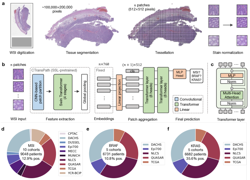
Figure 1: Workflow with pre-processing, model architecture and cohort overview. a) The data pre-processing pipeline with the steps whole slide image (WSI) digitization, tissue segmentation, tessellation into tiles, and stain normalization, b) the model architecture including the pre-trained feature extractor CTransPath and our transformer-based aggregation modules, and c) details of the transformer layer architecture. d) Overview of the 10 MSI cohorts used in this study with e) and f) the subsets of five cohorts with BRAF and KRAS annotations, respectively.

2.1 Model description

Our biomarker prediction pipeline consists of three steps (Figure 1): i) the data pre-processing pipeline (Figure 1a), ii) the transformer-based feature extractor, and iii) the transformer-based aggregation module that yields the final prediction from the embeddings of all patches of a whole-slide image (WSI) (Figure 1b).

In the pre-processing pipeline, tissue regions are segmented using RGB thresholding and Canny edge detection (Canny, 1986) to detect background and blurry regions. We include all tiles from a WSI, i.e., both tumor and healthy tissue tiles, thus reducing the burden of manual annotations when applying the algorithm. Subsequently, the WSI is tessellated into tiles of size 512$\times$512 pixels at 20$\times$ magnification with a resolution of 0.5 microns per pixel. To reduce the impact of the staining color on the model generalization, all tiles are stain-normalized with Macenko’s color deconvolution algorithm (Macenko et al., 2009) using a tile from the DACHS cohort as a reference image (Figure A.1).

We extract feature representations of dimension 768 for every tile using the CTransPath model (Wang et al., 2022). (Figure 1b). The model architecture is based on a Swin Transformer (Liu et al., 2021) that combines the hierarchical structure of CNNs with the global self-attention modules of transformers by computing self-attention in a sliding-window fashion. Similar to CNNs, these are stacked to increase the receptive field in every stage. CTransPath consists of three convolutional layers at the beginning to facilitate local feature extraction and improve training stability (Wang et al., 2022), followed by four Swin Transformer stages. Wang et al. (2022) trained the network using an unsupervised contrastive loss on data from TCGA and PAIP (Kim et al., 2021) from multiple organs and provided the weights for public use. The embeddings for each tile are stored for the subsequent training procedure.

The final part of the model takes all patches of a WSI as input and predicts one biomarker for all input patches in a weakly supervised manner (Figure 1b). Common attention-based MIL approaches (Ilse et al., 2018) use a small neural network, which mostly consists of two layers, to compute patch importance based on the embeddings. Each weight is computed based on one patch and finally, all weights are normalized over the input elements. In contrast to this, in our model, the patch embeddings are passed into a transformer network using multi-headed self-attention that considers the patch embeddings as a sequence and relates each element to every other element. In particular, assuming that $x\in\mathbb{R}^{n\times d}$ is the input sequence representing a WSI with $n$ patch embeddings of dimension $d$, the self-attention (SA) layer computes a query-key product in the following way

$$\mathrm{SA}(Q,K,V)=\mathrm{softmax}\left(\frac{QK^{T}}{\sqrt{d_{k}}}\right)V,$$ (1)

where queries $Q\in\mathbb{R}^{n\times d_{k}}$, keys $K\in\mathbb{R}^{n\times d_{k}}$, and values $V\in\mathbb{R}^{n\times d_{v}}$ .These are computed from the input sequence $x$ by

$$Q=W_{Q}\cdot x,\quad K=W_{K}\cdot x,\quad V=W_{V}\cdot x,$$ (2)

where $W_{Q}\in\mathbb{R}^{d\times d_{k}}$, $W_{K}\in\mathbb{R}^{d\times d_{k}}$, and $W_{V}\in\mathbb{R}^{d\times d_{v}}$ are learnable parameters. Multi-headed self-attention (MSA) applies self-attention in every head and concatenates the heads in a weighted manner:

$$\mathrm{MSA}(x) =\mathrm{concat}(\mathrm{head}_{1},...,\mathrm{head}_{h})\cdot W_{O},$$ (3)

$$\text{where}\ \mathrm{head}_{i} =\mathrm{SA}(Q^{(i)},K^{(i)},V^{(i)})\ \text{for}\ i\in\{1,...,h\}$$ (4)

and $W_{O}\in\mathbb{R}^{hd_{v}\times d}$ is learnable. We choose a small transformer network architecture consisting of two layers with each eight heads ($h=8$), a latent dimension of $512$, and the same dimension for query, keys, and values. Therefore, the latent dimension of each head is $d_{v}=d_{k}=64$, such that $hd_{v}=8\cdot 64=512$.

Assuming that $n$ is the number of patches per WSI, the embeddings of each patch $i\in\{1,\dots,n\}$ are stacked to a sequence of dimension $n\times 768$ and are passed through a linear projection layer followed by the non-linear activation ReLU to reduce the dimension from $768$ to $512$. Subsequently, a class token is concatenated to the input, similar to the usage in vision transformers (Dosovitskiy et al., 2020), yielding an input of dimension $(n+1)\times 512$ that is passed to the transformer layer. In each transformer layer, a block of layer normalization and multi-headed self-attention is followed by a block of layer normalization and a multi-layer perceptron (MLP), with skip connections applied across each block (Figure 1c).

After the two transformer layers, the class token of size $1\times 512$ is passed into an MLP head. Depending on the number of class tokens used, this enables single-target or multi-target binary prediction. Instead of attaching a class token, all $n$ sequence elements could be averaged to a single sequence element of size $1\times 512$ and passed into the MLP head. The averaging approach achieves similar performance to the class token version (Table A.1), but we decided to use the class token for better interpretability of the attention heads. We also compared our model architecture to the existing transformer-based aggregation module TransMIL (Shao et al., 2021) (Table A.1).

2.2 Ethics statement

In this study, we retrospectively analyzed anonymized patient samples from multiple academic institutions. At each of the following sites, the respective ethics board has given consent to this analysis: DACHS, Epi700, MECC, MUNICH, NLCS, and QUASAR. At the following sites, specific ethics approval was not required for a retrospective analysis of anonymized samples: CPTAC, DUSSEL, TCGA, and YCR-BCIP. Our study adheres to STARD (Table A.2).

2.3 Cohort description

Through coordination by the MSIDETECT consortium (www.msidetect.eu), we have collected H&E tissue sections of 9,048 patients with CRC from 10 patient cohorts in total, including two public databases (Figure 1d-f). The cohorts obtained are as follows:

1. The public database “The Clinical Proteomic Tumor Analysis Consortium”, CPTAC (publicly available at https://pdc.cancer.gov/pdc/, USA) (Edwards et al., 2015; Vasaikar et al., 2019) which includes tumors of any stage;

2. DACHS (Darmkrebs: Chancen der Verhütung durch Screening, Southwest Germany) (Hoffmeister et al., 2015; Brenner et al., 2011), a large population-based case-control and patient cohort study on CRC, including samples of patients with stages I-IV from different laboratories in southwestern Germany coordinated by the German Cancer Research Center (Heidelberg, Germany);

3. The DUSSEL (DUSSELdorf, Germany) cohort, a case series of CRC tumors resected with curative intent and collected at the Marien-Hospital in Duesseldorf, Germany, between January 1990 and December 1995 (Grabsch et al., 2006);

4. Epi700 (Belfast, N. Ireland, UK) (Gray et al., 2017a, b), a population-based cohort of stage II and III colon cancers treated by surgical resection between 2003 and 2008;

5. MECC (Molecular Epidemiology of Colorectal Cancer, Israel) (Shulman et al., 2018), a population-based case-control study in northern Israel;

6. The MUNICH (Munich, Germany) CRC series, a case series collected at the Technical University of Munich in Germany.

7. The NLCS (Netherlands Cohort Study, The Netherlands) (van den Brandt et al., 1990; Offermans et al., 2022) cohort, which contains tissue samples obtained from patients with any tumor stage as part of the Rainbow-TMA consortium study;

8. QUASAR, the “Quick and Simple and Reliable” trial (Yorkshire, UK) investigating survival benefit of adjuvant chemotherapy in patients from the United Kingdom with mostly stage II tumors (Quirke and Morris, 2007; QUASAR Collaborative Group, 2007);

9. The public repository “The Cancer Genome Atlas”, TCGA (publicly available at https://portal.gdc.cancer.gov/, USA) (Cancer Genome Atlas Network, 2012; Isella et al., 2014) which includes tumors of any stage;

10. The YCR-BCIP (Yorkshire Cancer Research Bowel Cancer Improvement Programme, Yorkshire, United Kingdom [UK]), a population-based register of bowel cancer patients in Yorkshire, UK (West et al., 2021; Taylor et al., 2019).

Detailed clinicopathological variables are shown in Table A.3. In all cohorts, formalin-fixed paraffin-embedded (FFPE) tissue was used. Slides have been scanned at their respective centers. For each patient, either an MSI status or a dMMR status, obtained by PCR or IHC, respectively, is available. Although MSI status and dMMR status are not fully concordant (West et al., 2021), they are used interchangeably in clinical routine and grouped as a single category in this study. KRAS and BRAF mutational status are available for the cohorts DACHS, Epi700, NLCS, QUASAR, and TCGA.

2.4 Experimental setup and implementation details

We performed all experiments using five-fold cross-validation with in-domain validation and testing. In this cross-validation variant, in-domain validation and test set are split off the full data set, leaving three folds for training (Figure A.2). By also cycling the in-domain test set through the complete dataset, we evaluated our model on more representative test sets than when fixing one smaller set for the dataset. During training, the validation set was used to determine the best model, which was consecutively evaluated on the test set. We further evaluated our models on external cohorts outside the dataset used for cross-validation for out-of-domain testing.

The transformer models were trained with the AdamW (Loshchilov and Hutter, 2017) optimizer using weight decay and learning rate both of $2*10^{-5}$ . All models were trained for eight epochs with batch size of one for two reasons: first, the sequences of embeddings had different lengths due to the variable number of tiles per WSI and could thus not be stacked to mini-batches of equal length inputs; second, limits in GPU capacity (32GB) because of the quadratic complexity of the self-attention mechanism and the large number of tiles per slide (up to 12,000, Figure A.3). To account for the varying cohort size, we evaluated the models every 500 iterations for runs on single cohorts, and every 1000 iterations for runs on multiple cohorts.

For comparison, we implemented the attention-based MIL approach from Ilse et al. (2018), referred to as AttentionMIL. It provided the best results with Adam (Kingma and Ba, 2014) optimizer, $1*10^{-2}$ as weight decay value, along with the fit-one-cycle learning rate scheduling policy (Smith and Topin, 2019) with a maximum learning rate of $1*10^{-4}$, trained over 32 epochs, and the first 25% of the cycle with increasing learning rate.

2.5 Statistics and endpoints

We used the area under the receiver operator curve (AUROC) as our main evaluation metric. Since our data is naturally highly imbalanced with respect to the target variables MSI, BRAF, and KRAS (Figure 1d-e), we further used the area under the precision-recall curve (AUPRC) as a metric as this metric accounts better for class imbalances than the AUROC metric. The precision-recall curve relates the recall or specificity, i.e., the ratio of correctly positive predicted samples to all positive samples, to the precision, i.e., the ratio of correctly positive predicted samples to all positive predicted samples. For every experiment, we reported the mean and the standard deviation of respective five-fold cross-validations (Figure A.2). We split the dataset into patient-wise training, validation, and internal test sets stratified by the target label, thus ensuring that every patient can only occur in one of these sets. The external test sets always consisted of different cohorts to better quantify the generalization properties of our algorithms.

2.6 Visualization and explainability

The final prediction is retrieved via the class token that is attached to the input sequence. To visualize the contribution of each input patch, we employed attention rollout as introduced by Abnar and Zuidema (2020). To obtain the attention at the class token in the final layer, the attention maps of the preceding layers are multiplied recursively. Attention rollout thus quantifies to which extent each patch contributes to the final prediction in the class score. Additionally, we visualized the attention scores for each head in the transformer by taking the class token’s self-attention, i.e., the query and key product. All presented attention scores were normalized to the range $[0,1]$ and clamped to the lower and higher 5%-quantiles, respectively, for better visual interpretability.

To visualize whether a patch contributed towards a positive or negative classification outcome, we fed the patches one-by-one through the transformer and visualized the resulting classification scores of the model. These scores were naturally in the range $[0,1]$ and can thus be directly visualized without further normalizing or clamping of values.

2.7 Code availability

All source codes are available under an open-source license at https://github.com/KatherLab/marugoto/tree/transformer.

3 Results

3.1 A fully transformer-based MSI prediction outperforms the state-of-the-art

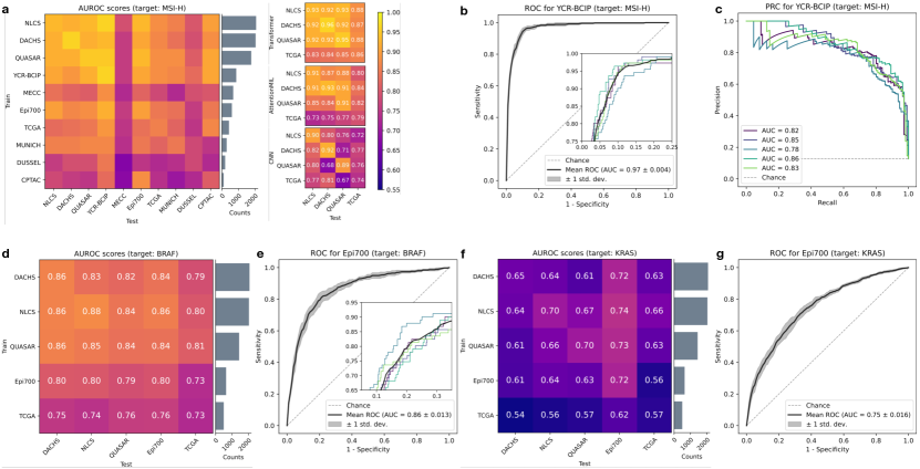
Figure 2: Evaluation of the prediction performance for the biomarkers MSI, BRAF, and KRAS in single-cohort and large-scale multi-centric experiments. Experimental results for MSI-H (a-c), BRAF (d,e), and KRAS (f,g) prediction: a) AUROC scores for single cohort experiments for all CRC cohorts ordered by size of the cohort. Each row shows the test performance of training on one cohort with the in-domain test results in the diagonal. Results for our transformer approach, AttentionMIL, and CNN approach (results taken from Echle et al.) are visualized separately. Note that compared to AttentionMIL and CNN, our transformer not only shows higher overall prediction accuracy but also better model generalizability, demonstrated by a smaller gap between internal and external testing cohorts. b) Receiver operator curve (ROC) for the model trained on four large cohorts DACHS, QUASAR, NLCS, and TCGA, tested on YCR-BCIP. c) Precision recall curve (PRC) for the model trained on four large cohorts DACHS, QUASAR, NLCS, and TCGA, tested on YCR-BCIP. d) AUROC scores for single cohort experiments. e) ROC for the model trained on four large cohorts DACHS, QUASAR, NLCS, TCGA and tested on Epi700. f) AUROC scores for single cohort experiments g) ROC for the model trained on four large cohorts DACHS, QUASAR, NLCS, TCGA and tested on Epi700. All values represent the mean of 5-fold cross-validation. Raw data for heatmap in a) in Table A.6.

We tested our pipeline on MSI prediction in 10 large cohorts of CRC patients in two ways: First, we trained the model on a single cohort and tested it on a held-out test set (in-domain) and on all other cohorts (external). We found that large cohorts, e.g., DACHS, QUASAR, or NLCS, achieved in-domain AUROCs close to 0.95 (Figure 2a). The model also achieved high performance close to 0.9 AUROC for early-onset CRC, i.e. CRC in patients younger than 50 years (Figure A.4). We compared this performance to the work by Echle et al. (2020) which updated the CNN-based feature extractor during training and used mean pooling as their patch aggregation function. Our approach outperformed the CNN-based approach on all four cohorts with the largest improvement on TCGA, increasing their results from 0.74 to 0.86 AUROC. Further, we also evaluated AttentionMIL by Ilse et al. (2018) with CTransPath as feature extractor yielding higher performance than the CNN-based approach on the large cohorts, but partly lower results on the external validation trained on the smaller cohort TCGA.

Second, we mirrored the experimental setup of Echle et al. (2020) and trained AttentionMIL and our fully transformer-based model on four large cohorts (DACHS, NLCS, QUASAR, and TCGA) and evaluated them on the external cohort YCR-BCIP. We used CTransPath as a feature extractor for both, AttentionMIL and our transformer-based model. The CNN-based approach from Echle et al. achieved an AUROC of 0.96, AttentionMIL yielded an AUROC of 0.96, and the fully transformer-based approach performed slightly better with an AUROC of 0.97 (Figure 2b). In particular, we obtained a sensitivity of 0.97 with a negative predictive value of 0.99 (Figure A.5). Moreover, a high mean AUPRC score of 0.83 showed that the transformer-based model achieved high sensitivity with relatively high precision despite a high class imbalance of 12.9% MSI-high samples on average across all cohorts (Figure 2c).

The classical patch-based approach by Echle et al. (2020) suffered from severe losses in performance upon external testing. The largest performance drop in the AUROC of 0.21 was observed by a model trained on the DACHS and tested on the QUASAR cohort. Our transformer model, however, reduced the performance loss for external testing to a maximum of 0.08 for training on the NLCS and testing on the TCGA cohort. In addition, AttentionMIL trained with the same transformer-based feature extractor also demonstrated better generalization capabilities compared to the classical patch-based approach with mean pooling. This suggests that self-supervised pretraining on histology data contributes positively towards better generalization.

In summary, these results show that a fully transformer-based approach yields a higher performance for biomarker prediction both on large cohorts (DACHS, QUASAR, and NLCS) as well as on smaller cohorts (TCGA). Perhaps more importantly from a clinical perspective, the transformer-based approach resulted in a better generalization performance and more reliable results, as the deviation between the external cohorts was smaller. We published all trained models for re-use, and further fine-tuning if needed.

3.2 The fully transformer-based model predicts multiple biomarkers in CRC

Next, we investigated whether the fully transformer-based model yields a similar high performance in other biomarker prediction tasks. Following the experimental setup for MSI prediction, we trained the model first on single cohorts evaluated on all other external cohorts and second on one fully merged multi-center cohort excluding only one cohort from the training set to constitute an external test set. In clinical routine workup for CRC, the biomarkers BRAF and KRAS are determined in addition to MSI. We tested whether and how well these were predictable on the DACHS, QUASAR, NLCS, TCGA, and Epi700 cohorts, where the Epi700 cohort served as an external test set in the multi-center run.

In the case of our larger cohorts, namely DACHS, QUASAR, and NLCS, single cohort training was already capable of achieving good results, with AUROCs of 0.86, 0.84, and 0.88, respectively (Figure 2d). The smaller cohorts achieved poorer results with wider standard deviations in AUROC across the five folds (0.1 and 0.08 for TCGA and Epi700 respectively, as compared to 0.02-0.03 for the larger cohorts). Nonetheless, the AUROC for the in-domain test using TCGA outperformed previous approaches with AUROCs of 0.57 (Fu et al., 2020) or 0.66 (Kather et al., 2020), and performed on par with more recent transformer-based methods with an AUROC of 0.73 (Reisenbüchler et al., 2022). The large multi-centric cohort yielded an AUROC of 0.86 (Figure 2e). Furthermore, we observed that the generalization gap from the internal test set to external cohorts was consistently small with the largest internal-to-external gap observed for the smallest cohort, TCGA. This was also the case in multi-centric evaluation, where the performance did not decrease from the internal to the external test cohort.

We observed similar results regarding the generalization when investigating KRAS as a target (Figure 2f-g), with an AUROC of 0.75 when trained on the multi-centric cohort, and AUROCs ranging from 0.57 to 0.72 for single cohorts. This is in line with state-of-the-art results (Kather et al., 2020; Fu et al., 2020; Reisenbüchler et al., 2022). While DL-based prediction performance for KRAS is still relatively low compared to MSI or BRAF, the results show that performance increases with the number of patients in the training cohort.

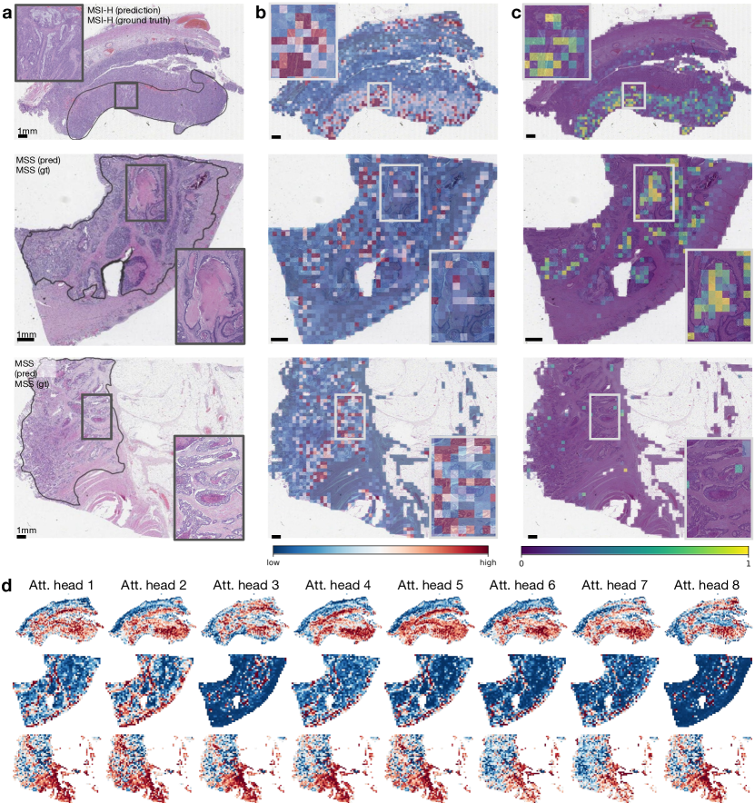
Figure 3: Attention and class score visualization for better model interpretability. a) Resection specimen from the external cohort YCR-BCIP. The three depicted slides are the same as in Echle et al. (2020). Tumor regions are outlined in black. b) Attention rollout per patch for our trained transformer-based feature aggregation model. Large values (red) signify a high contribution to the model’s prediction, smal values (blue) a low contribution. c) MSI classification scores per patch, where MSI-high is the positive class (scores larger then 0.5) and MS-stable is the negative class (scores lower than 0.5). d) The attention heatmaps from the all eight heads of the last layer. The methods used for visualization are describesd in the methods section. We used the model weights from the best performing fold of the multi-centric training on DACHS, NLCS, QUASAR, and TCGA.

Overall, these findings show that our model can predict multiple biomarkers relevant for routine diagnostics in CRC while highlighting the importance of large training cohorts to reach clinically relevant performance.

3.3 Fully transformer-based workflows are explainable

Ideally, DL-based biomarker predictions should be explainable to domain experts. To this end, we visualized how much each patch contributed to the final classification via attention rollout as well as whether it contributes towards a positive or negative classification (Figure 3a-c).

For better comparability, we used the same WSIs from the external cohort YCR-BCIP as had been used in a previous study (Echle et al., 2020) for these visualizations (Figure 3a). For all three cases, the majority of highly-contributing patches originate from tumor regions. In the MSI-high case, the mucinous region that is morphologically linked to MSI is correctly identified as important by high scores in the attention rollout as well as the patch-level classification. The MS-stable case in the second row of Figure 3a-c attributes high contributions to the model’s prediction to carcinoma regions. At the same time these patches all receive low classification scores yielding the correct classification result. Similarly, the second MS-stable case in the third row had highly contributing scores in the tumor region while having only low classification scores for all patches. Further tissue details that are morphologically related to MSI, such as solid growth patter, poor differentiation, or lymphocytes (Figure A.7) are highlighted in the attention heads of the last layer together with healthy tissue structures, such as the colon wall including muscle tissue or vessels (Figure 3d).

We observed that our model attributes a high level of attention not only to tissue regions, such as necrotic regions, but also larger blood vessels. Notably, such structures are not considered morphologically related to MSI from a pathologist’s perspective. Since these regions are particularly intensely stained by eosin, i.e., very pink or red, we suspect that the high color intensities lead to these responses. For all three cases, vessels in healthy tissue got higher attention scores than other healthy tissue regions but no high class scores, and therefore did not influence the MSI classification positively. However, the necrotic region highlighted in the second row of Figure 3 had high class scores similar to those seen in the model by Echle et al. (2020).

These examples showed that the model learns concepts relevant to MSI-high prediction and thus possess a high degree of explainability. Visualizing the attention rollout together with the classification scores demonstrates that relevant regions can receive high attention scores while the model can learn to ignore non-relevant regions or give them low class scores.

3.4 Fully transformer-based workflows are more data efficient

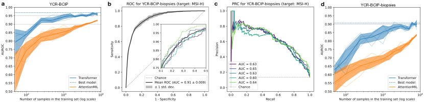
Figure 4: Analysis of data efficiency and model generalization to biopsies. a) AUROC scores on YCR-BCIP depending on the number of patients available for training. The samples were randomly drawn from the merged cohorts DACHS, NLCS, QUASAR, and TCGA. b) ROC for testing our model on YCR-BCIP-biopsies, trained on resections from DACHS, NLCS, QUASAR, and TCGA. c) PRC for testing our model on YCR-BCIP-biopsies, trained on resections from DACHS, NLCS, QUASAR, and TCGA. d) Analogue analysis to a) tested on YCR-BCIP-biopsies.

A longstanding problem in computational pathology is to determine the number of samples required for a given prediction task. This is primarily due to two reasons. First, it is unclear what the minimum required sample size is, and second, it is unclear if adding more samples improves performance, and if so, up to what point. To investigate this, we varied the number of patients in the training set and analyzed its impact on the test performance. Specifically, we merged all cohorts except for an external validation cohort, YCR-BCIP, resulting in a training set with 8181 patients from nine cohorts. We trained models using a fixed number of epochs and randomly sampled patients from the training set. All experiments were repeated five times and we reported the means and standard deviations of the results.

Our fully-transformer based model architecture achieved a mean testing AUROC value above 0.9 with 250 patients (in particular, an AUROC value of 0.92), while the AttentionMIL model exceeded an AUROC of 0.9 only with 4000 patients (Figure 4a). In a similar vein, our model surpassed the 0.95 mean testing AUROC with already 1500 patients, while AttentionMIL did not reach this performance. Hence, the transformer-based aggregation module helped the model to learn from data in a more efficient way than the attention mechanism. This may be due to the attention mechanism not contextualizing information from all input patches. Of note, above 1000 patients, the performance of the transformer-based model seems to slowly saturate, while the Attention mechanism continues to increase in performance with more patients but on a lower level.

Our fully transformer-based approach yielded high performance with a small sample size. Compared to an AttentionMIL-based approach, our approach is more data efficient in the regime of small numbers of patients. Looking at larger training numbers, we observed that performance increase is directly proportional to the number of patients for both approaches, but the fully transformer-based approach reaches equivalent performance already with much smaller datasets.

3.5 Fully transformer-based workflows result in clinical-grade performance on biopsies

Virtually all previous studies on biomarker prediction in CRC were performed using surgical resection slides. For this reason, commercially available MSI detection algorithms are intended to be used only with resection slides. However, recent clinical evidence shows that MSI-positive CRC patients require immunotherapy prior to surgery (Cercek et al., 2022; Chalabi et al., 2022) and hence need to be tested for MSI on biopsy material. We addressed this problem by training our model on resections from the cohorts, DACHS, QUASAR, NLCS, and TCGA, and evaluating it on biopsies from 1,502 patients with CRC of the YCIP-BCIP.

Our model yielded a mean AUROC score of 0.91 when externally validated on biopsies (Figure 4b). We outperformed existing approaches (0.78 by (Echle et al., 2020)) by far and achieved clinical-grade performance on biopsies after model training on resection specimen (Figure A.5). However, the mean AUPRC score of 0.63 however was lower than that of the external cohort YCR-BCIP for resections (0.83) (Figure 4c). Hence, choosing a classification threshold with high sensitivity, the ratio of correctly MSI positive predicted cases from all positive predicted cases was lower on biopsies compared to resections.

Our intended clinical use of this workflow is as follows (Figure 5): First, a patient attends a clinic either with suspected CRC or for routine CRC screening. A colonoscopy shows a suspicious tumor, which is evaluated histologically and found to be an adenocarcinoma. In many countries, this biopsy will then be tested for MSI/MMR status and BRAF and/or RAS mutation status. In practice, these procedures may take several days to even weeks. However, in low-or-middle-income countries, this might not happen at all. Based on the MSI, BRAF, and RAS status, the most suitable treatment approach will be chosen for the patient. For example, in patients with early (non-metastatic) CRC, the presence of MSI could qualify a patient for neoadjuvant immunotherapy followed by surgery with curative intent. Similarly, in the metastatic disease setting, the presence of MSI in the biopsy tissue would qualify a patient for palliative immunotherapy. Our algorithm could therefore speed up the step between taking the biopsy and the molecular determination of MSI-high status, thus enabling an earlier treatment with immunotherapy if indicated.

In summary, to the best of our knowledge, we developed the first DL-based MSI-high predictor for biopsies that achieves clinical-grade performance. In particular, this high performance was also observed for external tests and could therefore improve clinical routine and speed up treatment decisions.

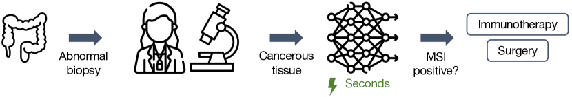
Figure 5: Envisioned clinical workflow for the proposed MSI-high classifier on biopsies. This assumes the system reaches a sufficient performance in additional external validation and is approved as a medical device. This workflow would only apply to non-metastatic disease. Neoadjuvant immunotherapy is not yet recommended by medical guidelines but is backed up by Phase-II clinical trials. Not shown: tissue preprocessing and scanning pipelines, and confirmatory tests of MSI after a positive deep learning-based pre-screening.

4 Discussion

The rollout of precision oncology to colorectal cancer patients promises gains in life expectancy (Hendricks et al., 2020). Unfortunately, however, its implementation still remains slow and patchy. One for this is that precision oncology biomarkers are complex, costly and require intricate instrumentation and expertise. DL is emerging as a possible solution for this problem (Shmatko et al., 2022; Bera et al., 2019). DL can extract biomarker information directly from routinely available material, thereby potentially providing cost savings (Kather et al., 2019). Using DL-based analysis of histopathology slides to extract biomarkers for oncology has become a common approach in the research setting in 2018 (Coudray et al., 2018). In turn, this has recently led to regulatory approval of multiple algorithms for clinical use. Some of these examples include a breast cancer survival prediction algorithm by Paige (New York, NY, USA), a method to predict survival in CRC by DoMore Diagnostics (Oslo, Norway), a method to predict MSI status in CRC by Owkin (Paris, France and New York, NY, USA), amongst others. However, existing DL biomarkers have some key limitations: it is debated whether or not their performance is sufficient for large-scale use, they do not necessarily generalize to any patient population, and finally, they are not approved for use on biopsy material, as the application of DL algorithms to biopsies typically results in much lower performance compared to application to surgical specimens (Echle et al., 2020).

A key reason for the limited performance of existing DL systems could be the fundamental limitations of the technology employed. Most studies between 2018 and 2020 used convolutional neural networks (CNNs) as their DL backbone (Ghaffari Laleh et al., 2022b), using publicly available information. Commercial products in the DL biomarker space are based on the same technology (Campanella et al., 2019; Svrcek et al., 2022; Kleppe et al., 2022). However, a new class of neural networks has recently started to replace CNNs: transformers. Originating from the field of natural language processing, transformers are a powerful tool to process sequences and leverage the potential of large amounts of data. Also in computer vision, transformers yield a higher accuracy for image classification in non-medical tasks (Dosovitskiy et al., 2020; Liu et al., 2021), are more robust to distortions in the input data (Ghaffari Laleh et al., 2022a) and provide more detailed explainability (Chen et al., 2022). These advantages of transformers compared to CNNs have the potential to translate into more accurate and more generalizable clinical biomarkers, but there is currently no evidence to support this.

In the present study, we developed the first fully transformer-based approach for biomarker prediction on whole-slide images of H&E-stained CRC tissue sections. Our model consists of a transformer-based feature extractor that was pretrained on histopathology images and a transformer-based aggregation module. In contrast to the state-of-the-art attention-based MIL approaches, the contribution of each patch was not only determined according to its feature embeddings but also contextualized with the feature embeddings of all other patches in the WSI via self-attention layers. Further, we presented the first large-scale evaluation of transformers in biomarker prediction on WSIs. We demonstrated that transformer-based approaches learned better from small amounts of data and were therefore more data-efficient than attention-based MIL approaches. At the same time, the performance increased proportionally with the number of training samples. Even though the performance seemed to plateau for MSI prediction, this suggests that larger training cohorts could lead to higher performance approaching clinical application, also for more challenging tasks such as the prediction of the BRAF and KRAS mutational status. Our large-scale evaluation also showed that MIL and in particular transformer-based approaches generalize much better than the existing CNN approaches. We proved this by training the model on single cohorts and testing the generalization on all other cohorts. These experiments showed that the transformer-based approach reduced the drop in AUROC to under 0.08, while the CNN-based approach dropped by more than 0.21 on some cohorts. Most importantly, our approach trained on resections did not only generalize well to external cohorts with resections but also to biopsies with a clinical-grade performance of 0.91 AUROC. A caveat of our experiments is that the ground truth is not perfect. Potentially, the DL model is performing better than stated in the paper because dMMR and MSI only agree around 92% of the time (West et al., 2021; NIC, ). Also, there are POLD1 and POLE mutant cases with a high mutation burden that are not identified by IHC, but behave clinically similar to MSI. Now the DL tests are high levels of performance so these small subpopulations may be important. Which are the cases that are picked up by the transforming algorithm that are not picked up by the old methods - this should be investigated in the future.

Our study still had some limitations: The focus of this study was to investigate the effect of handling the data with fully transformer-based approaches, especially in the context of large-scale multi-institutional data. Therefore, we did not optimize all details and hyperparameters of the architecture. Points for optimization in this direction would be finding a fitting positional encoding and tuning the architecture of the transformer network. Further, we applied Macenko stain normalization in the preprocessing pipeline since this reduced the generalization gap compared to no stain normalization, but other methods in this direction could be investigated to further reduce the generalization drop even further. Additionally, collecting biopsy samples from different hospitals, for multi-cohort training directly on biopsy data could potentially improve the performance of our model on biopsy material. This would also hold for the prediction of BRAF mutation status and, in particular, of RAS mutation status, where we observed the largest potential for improvement. In both targets, the performance was higher on the larger cohorts with around 2,000 patients and increased dramatically by training on multiple cohorts.

In summary, to the best of our knowledge, we presented the first fully transformer-based model to predict MSI on WSI from CRC with an AUROC of 0.97 on resections and 0.91 on biopsies, both obtained with external validation. Our model generalized better to unseen cohorts and was more data-efficient compared to existing state-of-the-art MIL or CNN approaches. By publishing all trained models, we enable researchers and clinicians to apply the automated MSI prediction tool in clinical practice, which we expect to bring the field of DL-based biomarkers a step closer to integration in the clinical workflow.

Additional Information

Disclosures

JNK reports consulting services for Owkin, France, Panakeia, UK, and DoMore Diagnostics, Norway and has received honoraria for lectures by MSD, Eisai, and Fresenius. NW has received fees for advisory board activities with BMS, Astellas, and Amgen, not related to this study. NW has received fees for advisory board activities with BMS, Astellas, and Amgen, not related to this study. PQ has received fees for advisory board activities with Roche and AMGEN and research funding from Roche through an Innovate UK National Pathology Imaging Consortium grant. HIG has received fees for advisory board activities by AstraZeneca and BMS, not related to this study. MST is a scientific advisor to Mindpeak and Sonrai Analytics, and has received honoraria recently from BMS, MSD, Roche, Sanofi and Incyte. He has received grant support from Phillips, Roche, MSD and Akoya. None of these disclosures are related to this work. No other potential disclosures are reported by any of the authors.

Author contributions

SJW, MB, TP, and JNK designed the concept of the study, MB, GPV supported with domain-related advice; DR, SJW, MB, and TP developed and evaluated a preliminary study, where DR implemented the methods; SJW, JMN prepared the data for this study, SJW implemented the methods and ran all experiments and evaluations; NW, PQ, HIG, PvdB, GGAH, SDR, KH, CG, MPE, ME, MB, DH, CR, TY, RL, JCAJ, KO, WM, RG, SBG, JKG, GR, JDB, DS, JJ, ML, MST, HB, and MH provided clinical and histopathological data; all authors provided clinical expertise and contributed to the interpretation of the results. SJW wrote the manuscript with JNK, and input from all other authors.

Acknowledgments

DACHS study: The authors thank the hospitals recruiting patients for the DACHS study and the cooperating pathology institutes. We thank the National Center for Tumor Diseases (NCT) Tissue Bank, Heidelberg, Germany, for managing, archiving, and processing tissue samples in the DACHS study.

We acknowledge the support of the Rainbow-TMA Consortium, especially the project group: PA van den Brandt, A zur Hausen, HI Grabsch, M van Engeland, LJ Schouten, J Beckervordersandforth (Maastricht University Medical Center, Maastricht, The Netherlands); PHM Peeters, PJ van Diest, HB Bueno de Mesquita (University Medical Center Utrecht, Utrecht, The Netherlands); J van Krieken, I Nagtegaal, B Siebers, B Kiemeney (Radboud University Medical Center, Nijmegen, The Netherlands); FJ van Kemenade, C Steegers, D Boomsma, GA Meijer (VU University Medical Center, Amsterdam, The Netherlands); FJ van Kemenade, B Stricker (Erasmus University Medical Center, Rotterdam, The Netherlands); L Overbeek, A Gijsbers (PALGA, the Nationwide Histopathology and Cytopathology Data Network and Archive, Houten, The Netherlands); and Rainbow-TMA collaborating pathologists, among others: A de Bruïne (VieCuri Medical Center, Venlo); JC Beckervordersandforth (Maastricht University Medical Center, Maastricht); J van Krieken, I Nagtegaal (Radboud University Medical Center, Nijmegen); W Timens (University Medical Center Groningen, Groningen); FJ van Kemenade (Erasmus University Medical Center, Rotterdam); MCH Hogenes (Laboratory for Pathology Oost-Nederland, Hengelo); PJ van Diest (University Medical Center Utrecht, Utrecht); RE Kibbelaar (Pathology Friesland, Leeuwarden); AF Hamel (Stichting Samenwerkende Ziekenhuizen Oost-Groningen, Winschoten); ATMG Tiebosch (Martini Hospital, Groningen); C Meijers (Reinier de Graaf Gasthuis/SSDZ, Delft); R Natté (Haga Hospital Leyenburg, The Hague); GA Meijer (VU University Medical Center, Amsterdam); JJTH Roelofs (Academic Medical Center, Amsterdam); RF Hoedemaeker (Pathology Laboratory Pathan, Rotterdam); S Sastrowijoto (Orbis Medical Center, Sittard); M Nap (Atrium Medical Center, Heerlen); HT Shirango (Deventer Hospital, Deventer); H Doornewaard (Gelre Hospital, Apeldoorn); JE Boers (Isala Hospital, Zwolle); JC van der Linden (Jeroen Bosch Hospital, Den Bosch); G Burger (Symbiant Pathology Center, Alkmaar); RW Rouse (Meander Medical Center, Amersfoort); PC de Bruin (St. Antonius Hospital, Nieuwegein); P Drillenburg (Onze Lieve Vrouwe Gasthuis, Amsterdam); C van Krimpen (Kennemer Gasthuis, Haarlem); JF Graadt van Roggen (Diaconessenhuis, Leiden); SAJ Loyson (Bronovo Hospital, The Hague); JD Rupa (Laurentius Hospital, Roermond); H Kliffen (Maasstad Hospital, Rotterdam); HM Hazelbag (Medical Center Haaglanden, The Hague); K Schelfout (Stichting Pathologisch en Cytologisch Laboratorium West-Brabant, Bergen op Zoom); J Stavast (Laboratorium Klinische Pathologie Centraal Brabant, Tilburg); I van Lijnschoten (PAMM Laboratory for Pathology and Medical Microbiology, Eindhoven); and K Duthoi (Amphia Hospital, Breda).

Funding

SJW and DR are supported by the Helmholtz Association under the joint research school “Munich School for Data Science - MUDS” and SJW is supported by the Add-on Fellowship of the Joachim Herz Foundation. JNK is supported by the German Federal Ministry of Health (DEEP LIVER, ZMVI1-2520DAT111), the Max-Eder-Programme of the German Cancer Aid (grant #70113864) and the German Academic Exchange Service (SECAI, 57616814). JNK and MH are funded by the German Federal Ministry of Education and Research (PEARL, 01KD2104C). PQ, NW, SD, and GH are supported by Yorkshire Cancer Research grants L386 and L394. PQ, HG, NW, JNK, and SD are supported in part by the National Institute for Health and Care Research (NIHR) Leeds Biomedical Research Centre. The views expressed are those of the author(s) and not necessarily those of the NHS, the NIHR, or the Department of Health and Social Care. PQ is also supported by an NIHR Senior Investigators award. Tumor tissue collection in the NLCS was done in the Rainbow-TMA study, which was financially supported by BBMRI-NL, a Research Infrastructure financed by the Dutch government (NWO 184.021.007 to PvdB). The analyses of MSI, BRAF, and KRAS in the NLCS were funded by The Dutch Cancer Society (KWF 11044 to PvdB). The DACHS study (HB, JCC, and MH) was supported by the German Research Council (BR 1704/6-1, BR 1704/6-3, BR 1704/6-4, CH 117/1-1, HO 5117/2-1, HO 5117/2-2, HE 5998/2-1, HE 5998/2-2, KL 2354/3-1, KL 2354/3-2, RO 2270/8-1, RO 2270/8-2, BR 1704/17-1 and BR 1704/17-2), the Interdisciplinary Research Program of the National Center for Tumor Diseases (NCT; Germany) and the German Federal Ministry of Education and Research (01KH0404, 01ER0814, 01ER0815, 01ER1505A and 01ER1505B). The study was further supported by project funding for the PEARL consortium from the German Federal Ministry of Education and Research (01KD2104A).

Appendix A Supplementary Materials

A.1 Supplementary Figures

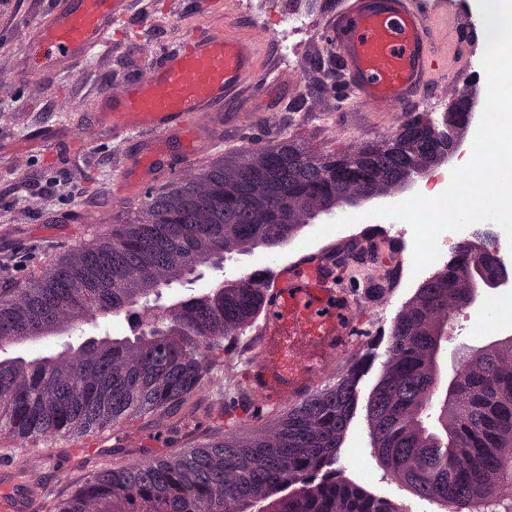
Figure A.1: Template tile used for stain normalization with Macenko’s method. The tile was taken from the DACHS cohort.

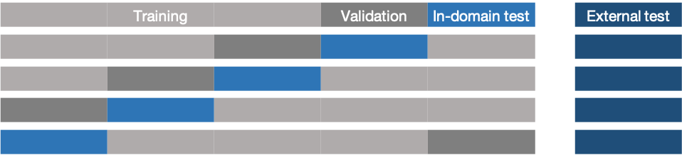
Figure A.2: Five-fold cross-validation scheme. Additionally to the standard use of five-fold cross-validation, we also cycle the in-domain test set through the whole dataset to get a more representative test evaluation of the dataset compared to splitting up a small in-domain test set beforehand.

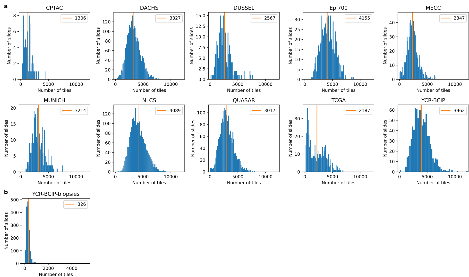
Figure A.3: Distribution of the number of tiles per slide for all cohorts. The mean of each distribution is highlighted in orange. a) Histogram of the distribution for all 10 cohorts of resections. b) Histogram of the distribution for the biopsy cohort.

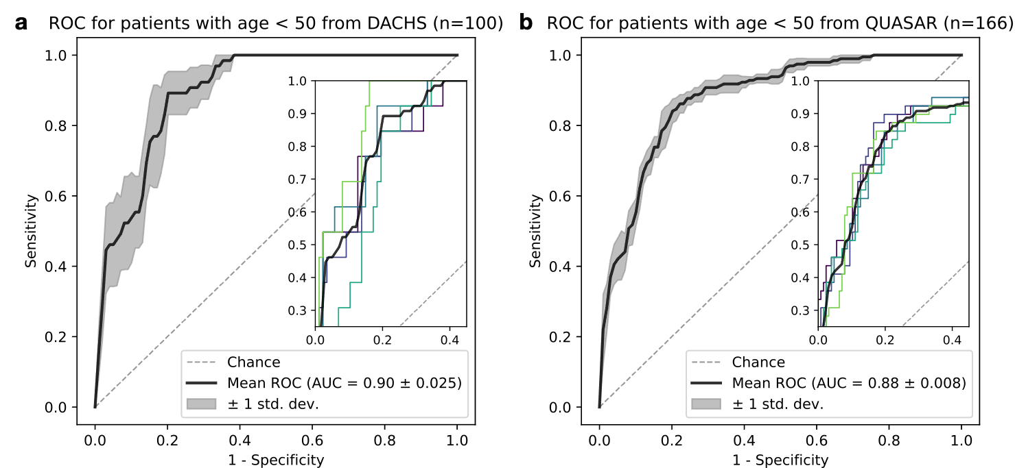
Figure A.4: Receiver operator curves for early onset cancer. a) External test on DACHS with 100 patients younger than 50 years, trained on QUASAR. b) External test on QUASAR with 166 patients younger than 50 years, trained on DACHS. Both cohorts were chosen because they contain a sufficient number of patients under 50 in contrast to the other cohorts in this study.

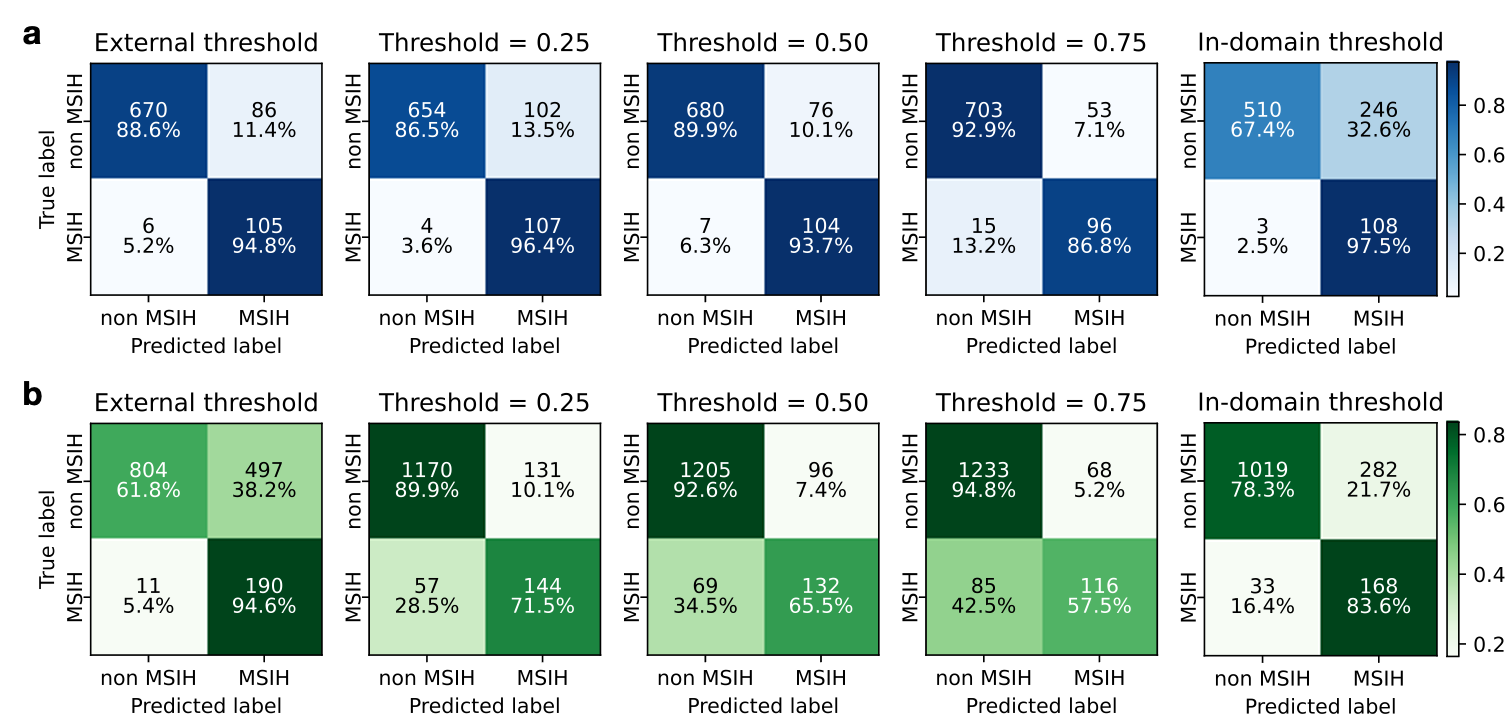
Figure A.5: Confusion matrix for different classification thresholds. First column shows the threshold determined on the external tests, such that 0.95 sensitivity is reached. Second to forth column show foxed thresholds (0.25, 0.5, 0.75, respectively). Last column shows the threshold determined on the in-domain test set, such that 0.95 sensitivity is reached. The results show the average of the model trained on the large multi-centric cohort DACHS, NLCS, QUASAR, and TCGA across all five folds. a) Results for the resection cohort YCR-BCIP. b) Results for the biopsy cohort YCR-BCIP-biopsies.

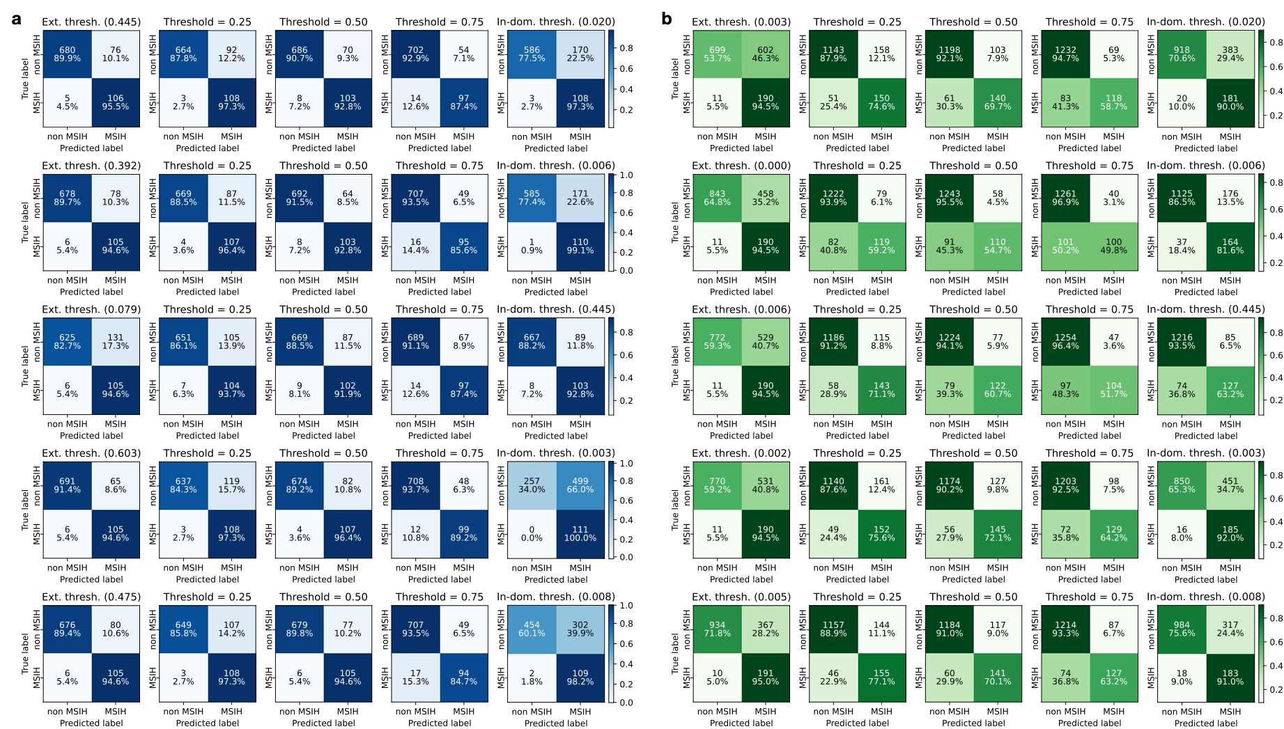
Figure A.6: Confusion matrix for different classification thresholds and all five folds. Similar to Figure A.5. Here the results of the models of each fold are shown in one row. a) Results for the resection cohort YCR-BCIP. b) Results for the biopsy cohort YCR-BCIP-biopsies.

Figure A.7: Manual annotation by a pathologist of the three test cases used for attention visualization from the YCR-BCIP cohort.

A.2 Supplementary Tables

Table A.1: Multi-cohort experiments with external validation on YCR-BCIP and YCR-BCIP-biopsies. The models were trained with the same pre-processing and feature extractor, only varying the architecture of the aggregation model. All models were trained with 5-fold cross validation.

ID	Train	Test	Target	Normali- zation	Feature Extraction	Aggregation Model	AUROC mean	AUROC std dev	AUPRC mean	AUPRC std dev	F1 (0.5) mean	F1 (0.5) std dev	F1 (gmean) mean	F1 (gmean) std dev
2.1.1	DACHS, NLCS, QUASAR, TCGA	DACHS, NLCS, QUASAR, TCGA	MSI-H	Macenko	CTransPath Wang et al. [2022]	Transformer with class token (ours)	0.95	0.0078	0.74	0.0284	0.83	0.1257	0.80	0.1370
2.2.1	DACHS, NLCS, QUASAR, TCGA	YCR-BCIP	MSI-H	Macenko	CTransPath Wang et al. [2022]	Transformer with class token (ours)	0.97	0.0041	0.83	0.0266	0.83	0.1145	0.84	0.1108
2.3.1	DACHS, NLCS, QUASAR, TCGA	YCR-BCIP-biopsies	MSI-H	Macenko	CTransPath Wang et al. [2022]	Transformer with class token (ours)	0.91	0.0094	0.63	0.0149	0.77	0.1616	0.74	0.1622
2.1.2	DACHS, NLCS, QUASAR, TCGA	DACHS, NLCS, QUASAR, TCGA	MSI-H	Macenko	CTransPath Wang et al. [2022]	Transformer with global averaging (ours)	0.95	0.0091	0.76	0.0224	0.83	0.1268	0.81	0.1322
2.2.2	DACHS, NLCS, QUASAR, TCGA	YCR-BCIP	MSI-H	Macenko	CTransPath Wang et al. [2022]	Transformer with global averaging (ours)	0.97	0.0042	0.84	0.0131	0.82	0.1272	0.83	0.1191
2.3.2	DACHS, NLCS, QUASAR, TCGA	YCR-BCIP-biopsies	MSI-H	Macenko	CTransPath Wang et al. [2022]	Transformer with global averaging (ours)	0.91	0.0078	0.64	0.0206	0.75	0.1795	0.74	0.1582
2.1.3	DACHS, NLCS, QUASAR, TCGA	DACHS, NLCS, QUASAR, TCGA	MSI-H	Macenko	CTransPath Wang et al. [2022]	AttentionMIL Ilse et al. [2018]	0.94	0.0103	0.71	0.0184	0.79	0.1477	0.77	0.1543
2.2.3	DACHS, NLCS, QUASAR, TCGA	YCR-BCIP	MSI-H	Macenko	CTransPath Wang et al. [2022]	AttentionMIL Ilse et al. [2018]	0.96	0.0025	0.80	0.0101	0.78	0.1413	0.82	0.1202
2.3.3	DACHS, NLCS, QUASAR, TCGA	YCR-BCIP-biopsies	MSI-H	Macenko	CTransPath Wang et al. [2022]	AttentionMIL Ilse et al. [2018]	0.90	0.0042	0.60	0.0154	0.76	0.1601	0.74	0.1595
2.1.4	DACHS, NLCS, QUASAR, TCGA	DACHS, NLCS, QUASAR, TCGA	MSI-H	Macenko	CTransPath Wang et al. [2022]	TransMILM Shao et al. [2021]	0.94	0.0101	0.72	0.0379	0.82	0.1387	0.79	0.1500
2.2.4	DACHS, NLCS, QUASAR, TCGA	YCR-BCIP	MSI-H	Macenko	CTransPath Wang et al. [2022]	TransMILM Shao et al. [2021]	0.96	0.0033	0.79	0.0200	0.84	0.1157	0.83	0.1155
2.3.4	DACHS, NLCS, QUASAR, TCGA	YCR-BCIP-biopsies	MSI-H	Macenko	CTransPath Wang et al. [2022]	TransMILM Shao et al. [2021]	0.89	0.0122	0.57	0.0178	0.72	0.2215	0.70	0.1736

Table A.2: STARD (STAndards for the Reporting of Diagnostic accuracy studies) Checklist.

Section & Topic	No	Item	Reported
TITLE OR ABSTRACT	1	Identification as a study of diagnostic accuracy using at least one measure of accuracy (such as sensitivity, specificity, predictive values, or AUC)	yes
ABSTRACT	2	Structured summary of study design, methods, results, and conclusions (for specific guidance, see STARD for Abstracts)	yes
INTRODUCTION	3	Scientific and clinical background, including the intended use and clinical role of the index test	yes
	4	Study objectives and hypotheses	yes
METHODS Study design	5	Whether data collection was planned before the index test and reference standard were performed (prospective study) or after (retrospective study)
METHODS Participants	6	Eligibility criteria
	7	On what basis potentially eligible participants were identified (such as symptoms, results from previous tests, inclusion in registry)
	8	Where and when potentially eligible participants were identified (setting, location and dates)
	9	Whether participants formed a consecutive, random or convenience series
METHODS Test methods	10a	Index test, in sufficient detail to allow replication	yes
	10b	Reference standard, in sufficient detail to allow replication	yes
	11	Rationale for choosing the reference standard (if alternatives exist)
	12a	Definition of and rationale for test positivity cut-offs or result categories of the index test, distinguishing pre-specified from exploratory	yes
	12b	Definition of and rationale for test positivity cut-offs or result categories of the reference standard, distinguishing pre-specified from exploratory
	13a	Whether clinical information and reference standard results were available to the performers/readers of the index test
	13b	Whether clinical information and index test results were available to the assessors of the reference standard
METHODS Analysis	14	Methods for estimating or comparing measures of diagnostic accuracy	yes
	15	How indeterminate index test or reference standard results were handled
	16	How missing data on the index test and reference standard were handled	yes
	17	Any analyses of variability in diagnostic accuracy, distinguishing pre-specified from exploratory
	18	Intended sample size and how it was determined	yes
RESULTS Participants	19	Flow of participants, using a diagram
	20	Baseline demographic and clinical characteristics of participants	yes
	21a	Distribution of severity of disease in those with the target condition
	21b	Distribution of alternative diagnoses in those without the target condition	yes
	22	Time interval and any clinical interventions between index test and reference standard
RESULTS Test results	23	Cross tabulation of the index test results (or their distribution) by the results of the reference standard
	24	Estimates of diagnostic accuracy and their precision (such as 95% confidence intervals)	yes
	25	Any adverse events from performing the index test or the reference standard
DISCUSSION	26	Study limitations, including sources of potential bias, statistical uncertainty, and generalisability	yes
	27	Implications for practice, including the intended use and clinical role of the index test
OTHER INFORMATION	28	Registration number and name of registry
	29	Where the full study protocol can be accessed
	30	Sources of funding and other support; role of funders	yes

Table A.3: Patient cohorts used in this study and their characteristics. Clinico-pathological data were provided by the respective study principal investigators. In all cases, the TNM version from the original study registry was used. Information about the localization of the tumor was either provided as a binary variable (left-sided vs. right-sided) by the study site or assigned by the authors as follows: the cecum, ascending colon, hepatic flexure and transverse colon were defined as a right-sided tumor location whereas the splenic flexure, descending colon, sigmoid colon and rectum were defined as left-sided. *Number of patients before dropout of samples. **for the MECC cohort, these statistics refer to the cases with available MSI/dMMR status only.

	CPTAC	DACHS	DUSSEL	Epi700	MECC**	MUNICH	NLCS	QUASAR	TCGA	YCR-BCIP
Origin	United States	Germany	Germany	Northern Ireland	Israel	Germany	Netherlands	United Kingdom	United States	United Kingdom
Number of patients*	110	2448	330	657	683	292	2452	2190	632	889
WSI format	SVS	SVS	SVS	SVS	TIF	SVS	TIFF/SVS	SVS	SVS	SVS
MSI-H/dMMR ground truth	MuTect2	PCR 3-plex	IHC 2-plex	PCR/IHC consensus	PCR 5-plex	IHC 4-plex	IHC 2-plex	IHC 4-plex or IHC 2-plex	PCR 5-plex	IHC 4-plex
MSI-H/dMMR, n (%)	24 (22%)	210 (9%)	45 (14%)	134 (20%)	106 (16%)	34 (12%)	259 (11%)	246 (11%)	65 (10%)	129 (15%)
MSS/pMMR, n (%)	81 (74%)	1836 (75%)	268 (81%)	469 (71%)	577 (84%)	258 (88%)	2193 (89%)	1529 (70%)	392 (62%)	760 (85%)
Mean age at diagnosis (std. dev.)	65.67 (11.38)	68.46 (10.82)	68.57 (11.77)	70.63 (11.4)	69.8	56.1 (11.84)	73.71 (6.04)	62.20 (9.60)	66.42 (12.67)	70.31 (9.97)
Colon cancer, n (%)	110 (100%)	1488 (61%)	204 (62%)	659 (99.7%)	530 (78%)	N/A	1730 (71%)	1474 (67%)	341 (54%)	667 (75%)
Rectal cancer, n (%)	0 (0%)	960 (39%)	116 (35%)	2 (0.3%)	123 (18%)	N/A	722 (29%)	526 (24%)	118 (19%)	215 (24%)
Site unknown, n (%)	0 (0%)	0 (0%)	10 (3%)	0 (0%)	30 (4%)	N/A	0 (0%)	190 (9%)	173 (27%)	7 (1%)
Female, n (%)	65 (59%)	1012 (41%)	181 (55%)	303 (46%)	320 (47%)	132 (45%)	1079 (44%)	848 (39%)	292 (46%)	395 (44%)
Male, n (%)	45 (41%)	1436 (59%)	149 (45%)	358 (54%)	363 (53%)	160 (55%)	1373 (56%)	1334 (61%)	322 (51%)	494 (56%)
gender unknown, n (%)	0 (0%)	0 (0%)	0 (0%)	0 (0%)	0 (0%)	0 (0%)	0 (0%)	8 (0%)	18 (3%)	0 (0%)
UICC stage I, n (%)	12 (11%)	485 (20%)	76 (23%)	0 (0%)	94 (14%)	52 (18%)	485 (20%)	1 (0%)	76 (12%)	169 (19%)
UICC stage II, n (%)	42 (38%)	801 (33%)	138 (42%)	394 (60%)	335 (49%)	118 (40%)	918 (37%)	1988 (91%)	166 (26%)	317 (36%)
UICC stage III, n (%)	48 (44%)	822 (34%)	110 (33%)	267 (40%)	123 (18%)	82 (28%)	641 (26%)	192 (9%)	140 (22%)	370 (42%)
UICC stage IV, n (%)	8 (7%)	337 (14%)	6 (2%)	0 (0%)	67 (10%)	39 (13%)	341 (14%)	0 (0%)	63 (10%)	0 (0%)
UICC stage unknown, n (%)	0 (0%)	3 (0%)	0 (0%)	0 (0%)	64 (9%)	1 (0%)	67 (3%)	9 (0%)	187 (30%)	33 (3%)
BRAF mutation, n (%)	N/A	151 (6%)	N/A	91 (14%)	49 (7%)	N/A	305 (12%)	120 (5%)	63 (10%)	75 (8%)
BRAF wild type, n (%)	N/A	1930 (79%)	N/A	550 (84%)	570 (83%)	N/A	1733 (71%)	1358 (62%)	471 (75%)	32 (4%)
BRAF status unknown, n (%)	N/A	367 (15%)	N/A	16 (2%)	64 (9%)	N/A	414 (17%)	712 (33%)	98 (15%)	782 (88%)
KRAS mutation, n (%)	N/A	677 (28%)	N/A	247 (38%)	252 (37%)	N/A	698 (28%)	555 (25%)	218 (34%)	N/A
KRAS wild type, n (%)	N/A	1397 (57%)	N/A	398 (61%)	405 (59%)	N/A	1335 (54%)	882 (40%)	316 (50%)	N/A
KRAS status unknown, n (%)	N/A	347 (15%)	N/A	12 (2%)	26 (4%)	N/A	419 (17%)	753 (35%)	98 (16%)	N/A
right-sided tumor, n (%)	58 (53%)	819 (33%)	72 (22%)	375 (57%)	238 (35%)	53 (18%)	946 (39%)	754 (34%)	176 (28%)	331 (37%)
left-sided tumor, n (%)	51 (46%)	1607 (66%)	226 (68%)	280 (42%)	409 (60%)	239 (82%)	1506 (61%)	1158 (53%)	248 (39%)	486 (55%)
sidedness unknown, n (%)	1 (1%)	22 (1%)	32 (10%)	6 (1%)	36 (5%)	0 (0%)	0 (0%)	150 (13%)	208 (33%)	72 (8%)
etiology	not specified	any	not specified	not specified	not specified	not specified	not specified	not specified	not specified	not specified

Table A.4: Multi-cohort experiments for BRAF and KRAS prediction with external validation on Epi700. All models were trained with 5-fold cross validation.

ID	Train	Test	Target	Normali- zation	Feature Extraction	Aggregation Model	AUROC mean	AUROC std dev	AUPRC mean	AUPRC std dev	F1 (0.5) mean	F1 (0.5) std dev	F1 (gmean) mean	F1 (gmean) std dev
3.1.1	DACHS, NLCS, QUASAR, TCGA	DACHS, NLCS, QUASAR, TCGA	BRAF	Macenko	CTransPath Wang et al. [2022]	Transformer with class token (ours)	0.86	0.0083	0.48	0.0241	0.69	0.2183	0.67	0.2093
3.2.1	DACHS, NLCS, QUASAR, TCGA	Epi700	BRAF	Macenko	CTransPath Wang et al. [2022]	Transformer with class token (ours)	0.86	0.0130	0.53	0.0387	0.73	0.1754	0.72	0.1678
3.3.1	DACHS, NLCS, QUASAR, TCGA	DACHS, NLCS, QUASAR, TCGA	KRAS	Macenko	CTransPath Wang et al. [2022]	Transformer with class token (ours)	0.69	0.0162	0.54	0.0119	0.64	0.1332	0.64	0.0832
3.1.2	DACHS, NLCS, QUASAR, TCGA	Epi700	KRAS	Macenko	CTransPath Wang et al. [2022]	Transformer with class token (ours)	0.75	0.0155	0.65	0.0209	0.67	0.0592	0.70	0.0577

Table A.5: Mean AUROC scores of 5-fold CV training on single cohorts, evaluated on all other cohorts. The training cohorts are listed in the columns and entries in the diagonal are in-domain test results.

Training cohort ($\downarrow$)	NLCS	Dachs	Quasar	YCR-BCIP	MECC	Epi700	TCGA	Munich	Duessel	CPTAC
NLCS	0.93	0.92	0.93	0.96	0.79	0.93	0.88	0.86	0.80	0.90
Dachs	0.92	0.96	0.92	0.93	0.76	0.91	0.87	0.84	0.79	0.88
Quasar	0.92	0.92	0.95	0.95	0.76	0.93	0.88	0.88	0.81	0.91
YCR-BCIP	0.91	0.89	0.92	0.96	0.76	0.91	0.88	0.87	0.83	0.91
MECC	0.84	0.82	0.81	0.88	0.73	0.82	0.78	0.73	0.79	0.80
Epi700	0.90	0.87	0.88	0.92	0.76	0.90	0.85	0.84	0.76	0.85
TCGA	0.83	0.84	0.85	0.89	0.75	0.84	0.86	0.82	0.75	0.87
Munich	0.86	0.86	0.87	0.87	0.74	0.85	0.82	0.85	0.78	0.75
Duessel	0.76	0.79	0.79	0.85	0.67	0.75	0.73	0.74	0.78	0.73
CPTAC	0.78	0.76	0.75	0.83	0.68	0.88	0.74	0.70	0.73	0.81

Table A.6: Data for the performance analysis with a varying number of patients in the training set. The experiments were repeated five times and we report mean and standard deviation.

Model →		Transformer (ours)		AttentionMIL		Transformer (ours)		AttentionMIL
Evaluation cohort →		YCR-BCIP		YCR-BCIP		YCR-BCIP-biopsies		YCR-BCIP-biopsies
	#patients	AUROC (mean)	AUROC (std. dev.)	AUROC (mean)	AUROC (std. dev.)	AUROC (mean)	AUROC (std. dev.)	AUROC (mean)	AUROC (std. dev.)
	50	0.792	0.0866	0.616	0.1252	0.629	0.0300	0.554	0.0640
	100	0.840	0.0180	0.744	0.0546	0.694	0.0628	0.604	0.0518
	250	0.923	0.0143	0.822	0.0281	0.811	0.0325	0.653	0.0372
	500	0.924	0.0173	0.838	0.0344	0.823	0.0306	0.673	0.0356
	1000	0.944	0.0148	0.854	0.0257	0.853	0.0441	0.695	0.0235
	1500	0.951	0.0130	0.865	0.0134	0.869	0.0175	0.716	0.0273
	2000	0.946	0.0046	0.881	0.0117	0.882	0.0213	0.737	0.0201
	3000	0.954	0.0066	0.890	0.0057	0.888	0.0122	0.755	0.0217
	4000	0.950	0.0065	0.901	0.0050	0.877	0.0151	0.775	0.0122
	5000	0.955	0.0056	0.906	0.0027	0.875	0.0119	0.789	0.0101
	6000	0.962	0.0096	0.913	0.0049	0.900	0.0155	0.810	0.0083
	7000	0.961	0.0027	0.918	0.0028	0.899	0.0034	0.823	0.0044
	8000	0.960	0.0080	0.922	0.0029	0.902	0.0221	0.836	0.0045

References

Kather et al. [2019]
Jakob Nikolas Kather, Alexander T Pearson, Niels Halama, Dirk Jäger,
Jeremias Krause, Sven H Loosen, Alexander Marx, Peter Boor, Frank Tacke,
Ulf Peter Neumann, Heike I Grabsch, Takaki Yoshikawa, Hermann Brenner, Jenny
Chang-Claude, Michael Hoffmeister, Christian Trautwein, and Tom Luedde.
Deep learning can predict microsatellite instability directly from
histology in gastrointestinal cancer.
Nat. Med., 25(7):1054–1056, July 2019.
Cao et al. [2020]
Rui Cao, Fan Yang, Si-Cong Ma, Li Liu, Yu Zhao, Yan Li, De-Hua Wu, Tongxin
Wang, Wei-Jia Lu, Wei-Jing Cai, Hong-Bo Zhu, Xue-Jun Guo, Yu-Wen Lu, Jun-Jie
Kuang, Wen-Jing Huan, Wei-Min Tang, Kun Huang, Junzhou Huang, Jianhua Yao,
and Zhong-Yi Dong.
Development and interpretation of a pathomics-based model for the
prediction of microsatellite instability in colorectal cancer.
Theranostics, 10(24):11080–11091,
September 2020.
Echle et al. [2020]
Amelie Echle, Heike Irmgard Grabsch, Philip Quirke, Piet A van den Brandt,
Nicholas P West, Gordon G A Hutchins, Lara R Heij, Xiuxiang Tan, Susan D
Richman, Jeremias Krause, Elizabeth Alwers, Josien Jenniskens, Kelly
Offermans, Richard Gray, Hermann Brenner, Jenny Chang-Claude, Christian
Trautwein, Alexander T Pearson, Peter Boor, Tom Luedde, Nadine Therese Gaisa,
Michael Hoffmeister, and Jakob Nikolas Kather.
Clinical-Grade detection of microsatellite instability in
colorectal tumors by deep learning.
Gastroenterology, 159(4):1406–1416.e11,
October 2020.
Bilal et al. [2021]
M Bilal, S E A Raza, A Azam, S Graham, M Ilyas, and others.
Development and validation of a weakly supervised deep learning
framework to predict the status of molecular pathways and key mutations in
colorectal ….
The Lancet Digital, 2021.
Lee et al. [2021]
Sung Hak Lee, In Hye Song, and Hyun-Jong Jang.
Feasibility of deep learning-based fully automated classification of
microsatellite instability in tissue slides of colorectal cancer.
Int. J. Cancer, 149(3):728–740, August
2021.
Schirris et al. [2022]
Yoni Schirris, Efstratios Gavves, Iris Nederlof, Hugo Mark Horlings, and Jonas
Teuwen.
DeepSMILE: Contrastive self-supervised pre-training benefits MSI
and HRD classification directly from H&E whole-slide images in
colorectal and breast cancer.
Med. Image Anal., 79:102464, July 2022.
Schrammen et al. [2022]
Peter Leonard Schrammen, Narmin Ghaffari Laleh, Amelie Echle, Daniel Truhn,
Volkmar Schulz, Titus J Brinker, Hermann Brenner, Jenny Chang-Claude,
Elizabeth Alwers, Alexander Brobeil, Matthias Kloor, Lara R Heij, Dirk
Jäger, Christian Trautwein, Heike I Grabsch, Philip Quirke, Nicholas P
West, Michael Hoffmeister, and Jakob Nikolas Kather.
Weakly supervised annotation-free cancer detection and prediction of
genotype in routine histopathology.
J. Pathol., 256(1):50–60, January 2022.
Yamashita et al. [2021]
Rikiya Yamashita, Jin Long, Teri Longacre, Lan Peng, Gerald Berry, Brock
Martin, John Higgins, Daniel L Rubin, and Jeanne Shen.
Deep learning model for the prediction of microsatellite instability
in colorectal cancer: a diagnostic study.
Lancet Oncol., 22(1):132–141, January
2021.
Jang et al. [2020]
Hyun-Jong Jang, Ahwon Lee, J Kang, In Hye Song, and Sung Hak Lee.
Prediction of clinically actionable genetic alterations from
colorectal cancer histopathology images using deep learning.
World J. Gastroenterol., 26(40):6207–6223, October 2020.
Benson et al. [2018]
Al B Benson, Alan P Venook, Mahmoud M Al-Hawary, Lynette Cederquist, Yi-Jen
Chen, Kristen K Ciombor, Stacey Cohen, Harry S Cooper, Dustin Deming, Paul F
Engstrom, Ignacio Garrido-Laguna, Jean L Grem, Axel Grothey, Howard S
Hochster, Sarah Hoffe, Steven Hunt, Ahmed Kamel, Natalie Kirilcuk, Smitha
Krishnamurthi, Wells A Messersmith, Jeffrey Meyerhardt, Eric D Miller, Mary F
Mulcahy, James D Murphy, Steven Nurkin, Leonard Saltz, Sunil Sharma, David
Shibata, John M Skibber, Constantinos T Sofocleous, Elena M Stoffel, Eden
Stotsky-Himelfarb, Christopher G Willett, Evan Wuthrick, Kristina M Gregory,
and Deborah A Freedman-Cass.
NCCN guidelines insights: Colon cancer, version 2.2018.
J. Natl. Compr. Canc. Netw., 16(4):359–369, April 2018.
[11]
National institute for health and care excellence. (2020). colorectal cancer
[NICE guideline no. 151]. https://www.nice.org.uk/guidance/ng151.
Schmoll et al. [2012]
H J Schmoll, E Van Cutsem, A Stein, V Valentini, B Glimelius, K Haustermans,
B Nordlinger, C J van de Velde, J Balmana, J Regula, I D Nagtegaal, R G
Beets-Tan, D Arnold, F Ciardiello, P Hoff, D Kerr, C H Köhne, R Labianca,
T Price, W Scheithauer, A Sobrero, J Tabernero, D Aderka, S Barroso,
G Bodoky, J Y Douillard, H El Ghazaly, J Gallardo, A Garin, R Glynne-Jones,
K Jordan, A Meshcheryakov, D Papamichail, P Pfeiffer, I Souglakos, S Turhal,
and A Cervantes.
ESMO consensus guidelines for management of patients with colon and
rectal cancer. a personalized approach to clinical decision making.
Ann. Oncol., 23(10):2479–2516, October
2012.
Chalabi et al. [2022]
M Chalabi, Y L Verschoor, J van den Berg, K Sikorska, G Beets, A V Lent, M C
Grootscholten, A Aalbers, N Buller, H Marsman, and Others.
LBA7 neoadjuvant immune checkpoint inhibition in locally advanced
MMR-deficient colon cancer: The NICHE-2 study.
Ann. Oncol., 33:S1389, 2022.
Vacante et al. [2018]
Marco Vacante, Antonio Maria Borzì, Francesco Basile, and Antonio Biondi.
Biomarkers in colorectal cancer: Current clinical utility and future
perspectives.
World J Clin Cases, 6(15):869–881,
December 2018.
Lim et al. [2015]
C Lim, M S Tsao, L W Le, F A Shepherd, R Feld, R L Burkes, G Liu, S Kamel-Reid,
D Hwang, J Tanguay, G da Cunha Santos, and N B Leighl.
Biomarker testing and time to treatment decision in patients with
advanced nonsmall-cell lung cancer.
Ann. Oncol., 26(7):1415–1421, July 2015.
Svrcek et al. [2022]
M Svrcek, C Saillard, R Dubois, N Loiseau, and others.
920P blind validation of MSIntuit, an AI-based pre-screening
tool for MSI detection from colorectal cancer H&E slides.
Annals of, 2022.
Chalabi et al. [2020]
Myriam Chalabi, Lorenzo F Fanchi, Krijn K Dijkstra, José G Van den Berg,
Arend G Aalbers, Karolina Sikorska, Marta Lopez-Yurda, Cecile Grootscholten,
Geerard L Beets, Petur Snaebjornsson, Monique Maas, Marjolijn Mertz, Vivien
Veninga, Gergana Bounova, Annegien Broeks, Regina G Beets-Tan, Thomas R
de Wijkerslooth, Anja U van Lent, Hendrik A Marsman, Elvira Nuijten, Niels F
Kok, Maria Kuiper, Wieke H Verbeek, Marleen Kok, Monique E Van Leerdam, Ton N
Schumacher, Emile E Voest, and John B Haanen.
Neoadjuvant immunotherapy leads to pathological responses in
MMR-proficient and MMR-deficient early-stage colon cancers.
Nat. Med., 26(4):566–576, April 2020.
Bilal et al. [2022]
Mohsin Bilal, Robert Jewsbury, Ruoyu Wang, Hammam M AlGhamdi, Amina Asif, Mark
Eastwood, and Nasir Rajpoot.
An aggregation of aggregation methods in computational pathology.
November 2022.
Ilse et al. [2018]
Maximilian Ilse, Jakub Tomczak, and Max Welling.
Attention-based deep multiple instance learning.
In Jennifer Dy and Andreas Krause, editors, Proceedings of the
35th International Conference on Machine Learning, volume 80 of
Proceedings of Machine Learning Research, pages 2127–2136. PMLR,
2018.
Dosovitskiy et al. [2020]
Alexey Dosovitskiy, Lucas Beyer, Alexander Kolesnikov, Dirk Weissenborn,
Xiaohua Zhai, Thomas Unterthiner, Mostafa Dehghani, Matthias Minderer, Georg
Heigold, Sylvain Gelly, Jakob Uszkoreit, and Neil Houlsby.
An image is worth 16x16 words: Transformers for image recognition at
scale.
October 2020.
Liu et al. [2021]
Ze Liu, Yutong Lin, Yue Cao, Han Hu, Yixuan Wei, Zheng Zhang, Stephen Lin, and
Baining Guo.
Swin transformer: Hierarchical vision transformer using shifted
windows.
In Proceedings of the IEEE/CVF International Conference on
Computer Vision, pages 10012–10022, 2021.
He et al. [2022]
K He, C Gan, Z Li, I Rekik, Z Yin, W Ji, Y Gao, and others.
Transformers in medical image analysis: A review.
arXiv preprint arXiv, 2022.
Ghaffari Laleh et al. [2022a]
Narmin Ghaffari Laleh, Daniel Truhn, Gregory Patrick Veldhuizen, Tianyu Han,
Marko van Treeck, Roman D Buelow, Rupert Langer, Bastian Dislich, Peter Boor,
Volkmar Schulz, and Jakob Nikolas Kather.
Adversarial attacks and adversarial robustness in computational
pathology.
Nat. Commun., 13(1):5711, September
2022a.
Wang et al. [2022]
Xiyue Wang, Sen Yang, Jun Zhang, Minghui Wang, Jing Zhang, Wei Yang, Junzhou
Huang, and Xiao Han.
Transformer-based unsupervised contrastive learning for
histopathological image classification.
Med. Image Anal., 81:102559, July 2022.
Chen et al. [2022]
Richard J Chen, Chengkuan Chen, Yicong Li, Tiffany Y Chen, Andrew D Trister,
Rahul G Krishnan, and Faisal Mahmood.
Scaling vision transformers to gigapixel images via hierarchical
Self-Supervised learning.
In Proceedings of the IEEE/CVF Conference on Computer Vision
and Pattern Recognition, pages 16144–16155, 2022.
Shao et al. [2021]
Zhuchen Shao, Hao Bian, Yang Chen, Yifeng Wang, Jian Zhang, Xiangyang Ji, and
Yongbing Zhang.
TransMIL: Transformer based correlated multiple instance learning
for whole slide image classification.
In Advances in Neural Information Processing Systems,
volume 34, pages 2136–2147, June 2021.
Reisenbüchler et al. [2022]
Daniel Reisenbüchler, Sophia J. Wagner, Melanie Boxberg, and Tingying Peng.
Local attention graph-based transformer for multi-target genetic
alteration prediction.
In Linwei Wang, Qi Dou, P. Thomas Fletcher, Stefanie Speidel, and
Shuo Li, editors, Medical Image Computing and Computer Assisted
Intervention – MICCAI 2022, pages 377–386, Cham, 2022. Springer Nature
Switzerland.
ISBN 978-3-031-16434-7.
Ghaffari Laleh et al. [2022b]
Narmin Ghaffari Laleh, Hannah Sophie Muti, Chiara Maria Lavinia Loeffler,
Amelie Echle, Oliver Lester Saldanha, Faisal Mahmood, Ming Y Lu, Christian
Trautwein, Rupert Langer, Bastian Dislich, Roman D Buelow, Heike Irmgard
Grabsch, Hermann Brenner, Jenny Chang-Claude, Elizabeth Alwers, Titus J
Brinker, Firas Khader, Daniel Truhn, Nadine T Gaisa, Peter Boor, Michael
Hoffmeister, Volkmar Schulz, and Jakob Nikolas Kather.
Benchmarking weakly-supervised deep learning pipelines for whole
slide classification in computational pathology.
Med. Image Anal., 79:102474, July
2022b.
Canny [1986]
J Canny.
A computational approach to edge detection.
IEEE Trans. Pattern Anal. Mach. Intell., 8(6):679–698, June 1986.
Macenko et al. [2009]
Marc Macenko, Marc Niethammer, J S Marron, David Borland, John T Woosley,
Xiaojun Guan, Charles Schmitt, and Nancy E Thomas.
A method for normalizing histology slides for quantitative analysis.
In 2009 IEEE International Symposium on Biomedical Imaging:
From Nano to Macro. IEEE, June 2009.
Kim et al. [2021]
Yoo Jung Kim, Hyungjoon Jang, Kyoungbun Lee, Seongkeun Park, Sung-Gyu Min,
Choyeon Hong, Jeong Hwan Park, Kanggeun Lee, Jisoo Kim, Wonjae Hong, Hyun
Jung, Yanling Liu, Haran Rajkumar, Mahendra Khened, Ganapathy Krishnamurthi,
Sen Yang, Xiyue Wang, Chang Hee Han, Jin Tae Kwak, Jianqiang Ma, Zhe Tang,
Bahram Marami, Jack Zeineh, Zixu Zhao, Pheng-Ann Heng, Rüdiger Schmitz,
Frederic Madesta, Thomas Rösch, Rene Werner, Jie Tian, Elodie Puybareau,
Matteo Bovio, Xiufeng Zhang, Yifeng Zhu, Se Young Chun, Won-Ki Jeong, Peom
Park, and Jinwook Choi.
PAIP 2019: Liver cancer segmentation challenge.
Med. Image Anal., 67:101854, January 2021.
Edwards et al. [2015]
Nathan J Edwards, Mauricio Oberti, Ratna R Thangudu, Shuang Cai, Peter B
McGarvey, Shine Jacob, Subha Madhavan, and Karen A Ketchum.
The CPTAC data portal: A resource for cancer proteomics research.
J. Proteome Res., 14(6):2707–2713, June
2015.
Vasaikar et al. [2019]
Suhas Vasaikar, Chen Huang, Xiaojing Wang, Vladislav A Petyuk, Sara R Savage,
Bo Wen, Yongchao Dou, Yun Zhang, Zhiao Shi, Osama A Arshad, Marina A
Gritsenko, Lisa J Zimmerman, Jason E McDermott, Therese R Clauss, Ronald J
Moore, Rui Zhao, Matthew E Monroe, Yi-Ting Wang, Matthew C Chambers, Robbert
J C Slebos, Ken S Lau, Qianxing Mo, Li Ding, Matthew Ellis, Mathangi
Thiagarajan, Christopher R Kinsinger, Henry Rodriguez, Richard D Smith,
Karin D Rodland, Daniel C Liebler, Tao Liu, Bing Zhang, and Clinical
Proteomic Tumor Analysis Consortium.
Proteogenomic analysis of human colon cancer reveals new therapeutic
opportunities.
Cell, 177(4):1035–1049.e19, May 2019.
Hoffmeister et al. [2015]
Michael Hoffmeister, Lina Jansen, Anja Rudolph, Csaba Toth, Matthias Kloor,
Wilfried Roth, Hendrik Bläker, Jenny Chang-Claude, and Hermann Brenner.
Statin use and survival after colorectal cancer: the importance of
comprehensive confounder adjustment.
J. Natl. Cancer Inst., 107(6):djv045, June
2015.
Brenner et al. [2011]
Hermann Brenner, Jenny Chang-Claude, Christoph M Seiler, and Michael
Hoffmeister.
Long-term risk of colorectal cancer after negative colonoscopy.
J. Clin. Oncol., 29(28):3761–3767,
October 2011.
Grabsch et al. [2006]
Heike Grabsch, Mit Dattani, Lisa Barker, Nicola Maughan, Karen Maude, Olaf
Hansen, Helmut E Gabbert, Phil Quirke, and Wolfram Mueller.
Expression of DNA double-strand break repair proteins ATM and
BRCA1 predicts survival in colorectal cancer.
Clin. Cancer Res., 12(5):1494–1500, March
2006.
Gray et al. [2017a]
Ronan T Gray, Maurice B Loughrey, Peter Bankhead, Chris R Cardwell, Stephen
McQuaid, Roisin F O’Neill, Kenneth Arthur, Victoria Bingham, Claire McGready,
Anna T Gavin, Jacqueline A James, Peter W Hamilton, Manuel Salto-Tellez,
Liam J Murray, and Helen G Coleman.
Statin use, candidate mevalonate pathway biomarkers, and colon cancer
survival in a population-based cohort study.
Br. J. Cancer, 116(12):1652–1659, June
2017a.
Gray et al. [2017b]
Ronan T Gray, Marie M Cantwell, Helen G Coleman, Maurice B Loughrey, Peter
Bankhead, Stephen McQuaid, Roisin F O’Neill, Kenneth Arthur, Victoria
Bingham, Claire McGready, Anna T Gavin, Chris R Cardwell, Brian T Johnston,
Jacqueline A James, Peter W Hamilton, Manuel Salto-Tellez, and Liam J Murray.
Evaluation of PTGS2 expression, PIK3CA mutation, aspirin use and
colon cancer survival in a Population-Based cohort study.
Clin. Transl. Gastroenterol., 8(4):e91,
April 2017b.
Shulman et al. [2018]
Katerina Shulman, Ofra Barnett-Griness, Vered Friedman, Joel K Greenson,
Stephen B Gruber, Flavio Lejbkowicz, and Gad Rennert.
Outcomes of chemotherapy for microsatellite Instable-High
metastatic colorectal cancers.
JCO Precis Oncol, 2, July 2018.
van den Brandt et al. [1990]
P A van den Brandt, R A Goldbohm, P van ’t Veer, A Volovics, R J Hermus, and
F Sturmans.
A large-scale prospective cohort study on diet and cancer in the
netherlands.
J. Clin. Epidemiol., 43(3):285–295, 1990.
Offermans et al. [2022]
Kelly Offermans, Josien Ca Jenniskens, Colinda Cjm Simons, Iryna Samarska,
Gregorio E Fazzi, Kim M Smits, Leo J Schouten, Matty P Weijenberg, Heike I
Grabsch, and Piet A van den Brandt.
Expression of proteins associated with the warburg-effect and
survival in colorectal cancer.
Hip Int., 8(2):169–180, March 2022.
Quirke and Morris [2007]
P Quirke and E Morris.
Reporting colorectal cancer.
Histopathology, 50(1):103–112, January
2007.
QUASAR Collaborative Group [2007]
QUASAR Collaborative Group.
Adjuvant chemotherapy versus observation in patients with colorectal
cancer: a randomised study.
Lancet, 370(9604):2020–2029, December
2007.
Cancer Genome Atlas
Network [2012]
Cancer Genome Atlas Network.
Comprehensive molecular characterization of human colon and rectal
cancer.
Nature, 487(7407):330–337, July 2012.
Isella et al. [2014]
Claudio Isella, Laura Cantini, Sara Erika Bellomo, and Enzo Medico.
TCGA CRC 450 dataset.
2014.
West et al. [2021]
Nicholas P West, Niall Gallop, Danny Kaye, Amy Glover, Caroline Young, Gordon
G A Hutchins, Scarlet F Brockmoeller, Alice C Westwood, Hannah Rossington,
Philip Quirke, and behalf of the Yorkshire Cancer Research Bowel Cancer
Improvement Programme group.
Lynch syndrome screening in colorectal cancer: results of a
prospective two-year regional programme validating the NICE diagnostics
guidance pathway across a 5.2 million population.
Histopathology, April 2021.
Taylor et al. [2019]
John Taylor, Penny Wright, Hannah Rossington, Jackie Mara, Amy Glover, Nick
West, Eva Morris, and Phillip Quirke.
Regional multidisciplinary team intervention programme to improve
colorectal cancer outcomes: study protocol for the yorkshire cancer research
bowel cancer improvement programme (YCR BCIP), 2019.
Loshchilov and Hutter [2017]
Ilya Loshchilov and Frank Hutter.
Decoupled weight decay regularization.
November 2017.
Kingma and Ba [2014]
Diederik P Kingma and Jimmy Ba.
Adam: A method for stochastic optimization.
December 2014.
Smith and Topin [2019]
Leslie N Smith and Nicholay Topin.
Super-convergence: very fast training of neural networks using large
learning rates.
In Artificial Intelligence and Machine Learning for
Multi-Domain Operations Applications, volume 11006, pages 369–386. SPIE,
May 2019.
Abnar and Zuidema [2020]
Samira Abnar and Willem Zuidema.
Quantifying attention flow in transformers.
May 2020.
Fu et al. [2020]
Yu Fu, Alexander W Jung, Ramon Viñas Torne, Santiago Gonzalez, Harald
Vöhringer, Artem Shmatko, Lucy Yates, Mercedes Jimenez-Linan, Luiza
Moore, and Moritz Gerstung.
Pan-cancer computational histopathology reveals mutations, tumor
composition and prognosis, 2020.
Kather et al. [2020]
Jakob Nikolas Kather, Lara R Heij, Heike I Grabsch, Chiara Loeffler, Amelie
Echle, Hannah Sophie Muti, Jeremias Krause, Jan M Niehues, Kai A J Sommer,
Peter Bankhead, Loes F S Kooreman, Jefree J Schulte, Nicole A Cipriani,
Roman D Buelow, Peter Boor, Nadi-Na Ortiz-Brüchle, Andrew M Hanby,
Valerie Speirs, Sara Kochanny, Akash Patnaik, Andrew Srisuwananukorn, Hermann
Brenner, Michael Hoffmeister, Piet A van den Brandt, Dirk Jäger,
Christian Trautwein, Alexander T Pearson, and Tom Luedde.
Pan-cancer image-based detection of clinically actionable genetic
alterations.
Nat Cancer, 1(8):789–799, August 2020.
Cercek et al. [2022]
Andrea Cercek, Melissa Lumish, Jenna Sinopoli, Jill Weiss, Jinru Shia, Michelle
Lamendola-Essel, Imane H El Dika, Neil Segal, Marina Shcherba, Ryan Sugarman,
Zsofia Stadler, Rona Yaeger, J Joshua Smith, Benoit Rousseau, Guillem
Argiles, Miteshkumar Patel, Avni Desai, Leonard B Saltz, Maria Widmar,
Krishna Iyer, Janie Zhang, Nicole Gianino, Christopher Crane, Paul B
Romesser, Emmanouil P Pappou, Philip Paty, Julio Garcia-Aguilar, Mithat
Gonen, Marc Gollub, Martin R Weiser, Kurt A Schalper, and Luis A Diaz.
PD-1 blockade in mismatch Repair–Deficient, locally advanced
rectal cancer.
N. Engl. J. Med., 386(25):2363–2376, June
2022.
Hendricks et al. [2020]
Alexander Hendricks, Anu Amallraja, Tobias Meißner, Peter Forster, Philip
Rosenstiel, Greta Burmeister, Clemens Schafmayer, Andre Franke, Sebastian
Hinz, Michael Forster, and Casey B Williams.
Stage IV colorectal cancer patients with high risk mutation
profiles survived 16 months longer with individualized therapies.
Cancers, 12(2), February 2020.
Shmatko et al. [2022]
Artem Shmatko, Narmin Ghaffari Laleh, Moritz Gerstung, and Jakob Nikolas
Kather.
Artificial intelligence in histopathology: enhancing cancer research
and clinical oncology.
Nat Cancer, 3(9):1026–1038, September
2022.
Bera et al. [2019]
Kaustav Bera, Kurt A Schalper, David L Rimm, Vamsidhar Velcheti, and Anant
Madabhushi.
Artificial intelligence in digital pathology - new tools for
diagnosis and precision oncology.
Nat. Rev. Clin. Oncol., August 2019.
Coudray et al. [2018]
Nicolas Coudray, Paolo Santiago Ocampo, Theodore Sakellaropoulos, Navneet
Narula, Matija Snuderl, David Fenyö, Andre L Moreira, Narges Razavian,
and Aristotelis Tsirigos.
Classification and mutation prediction from non-small cell lung
cancer histopathology images using deep learning.
Nat. Med., 24(10):1559–1567, October
2018.
Campanella et al. [2019]
Gabriele Campanella, Matthew G Hanna, Luke Geneslaw, Allen Miraflor, Vitor
Werneck Krauss Silva, Klaus J Busam, Edi Brogi, Victor E Reuter, David S
Klimstra, and Thomas J Fuchs.
Clinical-grade computational pathology using weakly supervised deep
learning on whole slide images.
Nat. Med., 25(8):1301–1309, August 2019.
Kleppe et al. [2022]
Andreas Kleppe, Ole-Johan Skrede, Sepp De Raedt, Tarjei S Hveem, Hanne A
Askautrud, Jørn E Jacobsen, David N Church, Arild Nesbakken, Neil A
Shepherd, Marco Novelli, Rachel Kerr, Knut Liestøl, David J Kerr, and
Håvard E Danielsen.
A clinical decision support system optimising adjuvant chemotherapy
for colorectal cancers by integrating deep learning and pathological staging
markers: a development and validation study, 2022.