Non-perturbative renormalization group analysis of nonlinear spiking networks

Abstract

The critical brain hypothesis posits that neural circuits may operate close to critical points of a phase transition, which has been argued to have functional benefits for neural computation. Theoretical and computational studies arguing for or against criticality in neural dynamics have largely relied on establishing power laws in neural data, while a proper understanding of critical phenomena requires a renormalization group (RG) analysis. However, neural activity is typically non-Gaussian, nonlinear, and non-local, rendering models that capture all of these features difficult to study using standard statistical physics techniques. We overcome these issues by adapting the non-perturbative renormalization group (NPRG) to work on network models of stochastic spiking neurons. Within a “local potential approximation,” we are able to calculate non-universal quantities such as the effective firing rate nonlinearity of the network, allowing improved quantitative estimates of network statistics. We also derive the dimensionless flow equation that admits universal critical points in the renormalization group flow of the model, and identify two important types of critical points: in networks with an absorbing state there is a fixed point corresponding to a non-equilibrium phase transition between sustained activity and extinction of activity, and in spontaneously active networks there is a physically meaningful complex valued critical point, corresponding to a discontinuous transition between high and low firing rate states. Our analysis suggests these fixed points are related to two well-known universality classes, the non-equilibrium directed percolation class, and the kinetic Ising model with explicitly broken symmetry, respectively.

There is little hope of understanding how each of the $\mathcal{O}(10^{11})$ neurons contributes to the functions of the brain KassAnnRevStats2018 . These neurons must operate amid constantly changing and noisy environmental conditions and internal conditions of an organism FaisalNatRevNeuro2008 , rendering neural circuitry stochastic and often far from equilibrium. Experimental work has demonstrated that neural circuitry can operate in many different regimes of activity rabinovich2006dynamical ; zhang1996representation ; laing2001stationary ; wimmer2014bump ; kim2017ring ; ermentrout1979mathematical ; bressloff2010metastable ; butler2012evolutionary ; SompolinskyPRL1988 ; dahmen2019second ; beggs2003neuronal ; buice2007field ; FriedmanPRL2012 ; kadmon2015transition , and theoretical and computational work suggests that transitions between these different operating regimes of collective activity may be sharp, akin to phase transitions observed in statistical physics. Some neuroscientists argue that circuitry in the brain is actively maintained close to critical points—the dividing lines between phases—as a means of minimizing reaction time to perturbations and switching between computations, or for maximizing information transmitted. This has become known as the “critical brain hypothesis” shew2011information ; BeggsFrontPhysio2012 ; FriedmanPRL2012 ; ShewTheNeuro2013 . While the hypothesis has garnered experimental and theoretical support in its favor, is has also become controversial, with many scientists arguing that key signatures of criticality, such as power law scaling, may be produced by non-critical systems touboul2010can ; touboul2017power , or are potentially artifacts of statistical inference in sub-sampled recordings nonnenmacher2017signatures ; levina2017subsampling .

The tools of non-equilibrium statistical physics have been built to investigate such dynamic collective activity. However, there are several obstacles to the application of these tools to neural dynamics: neurons are not arranged in translation-invariant lattices with simple nearest-neighbor connections, and neurons communicate with all-or-nothing signals called “spikes,” the statistics of which are very non-Gaussian. These are all features very unlike the typical systems studied in soft condensed matter physics, and hence methods developed to treat such systems often cannot be applied to models of neural activity without drastically simplifying neural models to fit these unrealistic assumptions.

Tools that have been somewhat successful at treating neural spiking activity on networks include mean-field theory, linear response theory, and diagrammatic perturbative calculations to correct these approximations OckerPloscb2017 ; stapmanns2020self ; KordovanArxiv2020 ; ocker2022dynamics . However, these tools break down when the synaptic connections between neurons are strong, particularly when the system is close to a bifurcation. A powerful approach for studying the statistical behavior of strongly coupled systems is the non-perturbative renormalization group (NPRG), which has been successfully used to study many problems in condensed matter physics CanetPRL2004 ; canet2005nonperturbative ; MachadoPRE2010 ; CanetJPhysA2011 ; RanconPRB2011 ; WinklerPRE2013 ; HomrighausenPRE2013 ; KlossPRE2014 ; balog2015activated ; canet2015fully ; JakubczykPRE2016 ; DuclutPRE2017 . However, because these methods have been developed for lattices or continuous media in which the fluctuations are driven by Gaussian noise, they cannot be straightforwardly applied to spiking network models. Previous work has studied phase transitions in neuron models primarily either through simulations, data analysis beggs2003neuronal ; FriedmanPRL2012 ; meshulam2019coarse , or by applying renormalization group methods to models from statistical mechanics that have been reinterpreted in a neuroscience context as firing rate models or coarse-grained activity states (e.g., “active” or “quiescent”) buice2007field ; bradde2017pca ; tiberi2022gell , but not spikes.

In this work we adapt the non-perturbative renormalization group method to apply to a stochastic spiking network model commonly used in neuroscience. We show that we are able to investigate both universal and non-universal properties of the spiking network statistics, even away from phase transitions, on both lattices and random networks, as depicted in Fig. 1. We begin by briefly reviewing the spiking network model and the types of phase transitions predicted by a mean-field analysis (Sec. I). We then introduce the core idea of the NPRG method and derive the flow equations for the spiking network model (Sec. II), which we use to calculate non-universal quantities like the effective nonlinearity that predicts how a neuron’s mean firing rate is related to its mean membrane potential. To investigate universal properties, we then present the rescaled RG flow equations and conditions under which non-trivial critical points exist (Sec. III). The properties of these critical points depend on an effective dimension $d$, which coincides with spatial dimension in nearest-neighbor networks. We end this report by discussing the implications of this work for current theoretical and experimental investigations of collective activity in spiking networks, both near and away from phase transitions (Sec. IV).

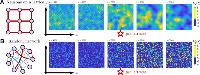
Figure 1: Dynamics of neurons on lattices versus networks can appear to differ substantially, depending on features like the statistics of synaptic connections between neurons and the signs of those synaptic connections. For example, A) shows the dynamics of a simulated network of excitatory neurons connected to their neighbors on a 2-dimensional lattice. Initially, the neurons fire asynchronously at intermediate rates. At $t=3333$ timesteps into the simulation, the gain of the neurons is increased (reflecting, for example, changes in attention of the organism), which creates two metastable states of high or low firing rate that drift through the network. In comparison, for the network of B) neurons are connected randomly with synaptic strengths of either sign. Because there is not spatial organization, it is not clear if the increase in gain creates metastable states of activity in the network, or if it merely increases the variance of the network. Network models like this have been studied extensively using approximate techniques like mean-field theory, but understanding the roles that stochastic fluctuations play in these systems demands the use of tools from the renormalization group (RG).

I Spiking network model

I.1 Model definition

We consider a network of $N$ neurons that stochastically fire action potentials, which we refer to as “spikes.” The probability that neuron $i$ fires $\dot{n}_{i}(t)dt$ spikes within a small window $[t,t+dt]$ is given by a counting process with expected rate $\phi(V_{i}(t))dt$, where $\phi(V)$ is a non-negative firing rate nonlinearity, conditioned on the current value of the membrane potential $V_{i}(t)$. We assume $\phi(V)$ is the same for all neurons, and for definiteness we will take the counting process to be Poisson or Bernoulli, though the properties of the critical points are not expected depend on this specific choice.

The membrane potential of each neuron obeys leaky dynamics,

$$\tau\frac{dV_{i}}{dt} =-(V_{i}-\mathcal{E}_{i})+\sum_{j=1}^{N}J_{ij}\dot{n}_{j}(t),$$ (1)

$$\dot{n}_{i}(t)dt \sim{\rm Poiss}[\phi(V_{i}(t))dt]$$ (2)

where $\tau$ is the membrane time constant, $\mathcal{E}_{i}$ is the rest potential, and $J_{ij}$ is the weight of the synaptic connection from pre-synaptic neuron $j$ to post-synaptic neuron $i$. We allow $J_{ii}$ to be non-zero in general to allow for, e.g., refractory effects that would otherwise be absent in this model (i.e., there is no hard reset of the membrane potential after a neuron fires a spike). For simplicity, we model the synaptic input as an instantaneous impulse, referred to as a “pulse coupled” network. It is straightforward to generalize $J_{ij}$ to a general a time-dependent linear filter of the incoming spikes, but this would complicate the upcoming calculations. Similarly, for technical reasons explained later, we restrict our analysis to symmetric networks, $J_{ij}=J_{ji}$.

I.2 Mean-field analysis and phase transitions

The stochastic system defined by Eqs. (1)-(2) cannot be solved in closed form, and understanding the statistical dynamics of these networks has historically been accomplished through simulations and approximate analytic or numerical calculations.

A qualitative picture of the dynamics of the model can often be obtained by a mean-field approximation in which fluctuations are neglected, such that $\langle\dot{n}_{i}(t)\rangle=\langle\phi(V_{i}(t))\rangle\approx\phi\left(\langle V_{i}(t)\rangle\right)$, and solving the resulting deterministic dynamics:

$$\tau\frac{d\langle V_{i}(t)\rangle}{dt} =-(\langle V_{i}(t)\rangle-\mathcal{E}_{i})+\sum_{j=1}^{N}J_{ij}\phi\left(\langle V_{j}(t)\rangle\right).$$ (3)

Equations of this form have long been a cornerstone of theoretical neuroscience, though often motivated phenomenologically, rather than as the mean-field approximation of a spiking network’s membrane potential dynamics. Many different types of dynamical behaviors and transitions among behaviors are possible depending on the properties of the connections $J_{ij}$ and nonlinearity $\phi(V)$ rabinovich2006dynamical , including bump attractors zhang1996representation ; laing2001stationary ; wimmer2014bump ; kim2017ring , pattern formation in networks of excitatory and inhibitory neurons ermentrout1979mathematical ; bressloff2010metastable ; butler2012evolutionary , transitions to chaos SompolinskyPRL1988 ; dahmen2019second , and avalanche dynamics beggs2003neuronal ; buice2007field ; FriedmanPRL2012 . Many networks admit steady-states for which $d\langle V_{i}\rangle/dt=0$ for all $i$ as $t\rightarrow\infty$. In this work we will focus on transitions from asynchronous steady states characterized by $\langle V_{i}(t)\rangle=0$ (or $\lim_{N\rightarrow\infty}N^{-1}\sum_{i=1}^{N}\langle V_{i}(t)\rangle=0$) to active states. If the rest potentials $\mathcal{E}_{i}$ are tuned to cancel out the mean-input to each neuron, then the transition from quiescent to active states is fluctuation-driven. For analytic $\phi(V)=\phi(0)+\phi^{\prime}(0)V+AV^{1+\beta^{-1}}+\dots$, where $V^{1+\beta^{-1}}$ is the lowest order nonlinear dependence (i.e., $\beta^{-1}>0$), we can estimate the dynamics of the mean membrane potentials when $\langle V\rangle$ is close to $0$ from above. In the subcritical or critical regimes in which $\langle V_{i}(t)\rangle$ decays to $0$, the projection of $\langle V_{i}(t)\rangle$ onto the eigenmode of $J_{ij}$ with the largest eigenvalue, $\Lambda_{\rm max}$, will have the slowest rate of decay, so we may approximate $\langle V_{i}(t)\rangle$ by the dynamics of this leading order mode:

$$\tau\frac{d\langle V\rangle}{dt} \approx-(1-\Lambda_{\rm max}\phi^{\prime}(0))\langle V\rangle+Ac\langle V\rangle^{1+\beta^{-1}}+\dots,$$

where $c$ is a constant depending on the eigenmode of $J_{ij}$ with eigenvalue $\Lambda_{\rm max}$. When the inverse response time $\xi_{\tau}^{-1}/\tau^{-1}\equiv 1-\Lambda_{\rm max}\phi^{\prime}(0)>0$ the solution decays to zero exponentially, whereas $\langle V(t)\rangle$ decays algebraically when $\xi_{\tau}^{-1}=0$:

$$\langle V(t)\rangle\sim\left\{\begin{array}[]{c}\exp(-t/\xi_{\tau}),~{}\xi_{\tau}^{-1}>0\\ t^{-\beta},~{}\xi_{\tau}=0\end{array}\right..$$ (4)

For $\xi_{\tau}^{-1}<0$ the zero solution of the mean-field equation becomes unstable. In networks with homogeneous excitatory couplings, non-zero steady-state solutions emerge (assuming $Ac<0$),

$$\langle V(\infty)\rangle\sim|1-\Lambda_{\rm max}\phi^{\prime}(0)|^{\beta},$$

with an exponential decay toward these values. Note that for even $\beta^{-1}\geq 2$ there are two solutions of opposite sign, whereas for odd $\beta^{-1}$ there is one real positive solution. Typically, $\beta^{-1}=1$ or $2$ for nonlinearities $\phi(y)$ commonly used in spiking network models. For random networks with synapses of either sign the behavior is more complicated, and is traditionally studied using the dynamic mean-field formalism. For symmetric networks like those we will focus on in this work, the analysis of Eq. (3) predicts a transition to a spin glass phase as the strength of the synaptic connections grows marti2018correlations .

This mean-field model can describe phase transitions in two important types of networks: i) “absorbing state networks”, for which $\phi(V)$ is $0$ when $V\leq 0$, and there are no fluctuations in activity once the network has reached this state; and ii) spontaneous networks, for which $\phi(0)\neq 0$ and neurons can stochastically fire even if the network has become quiescent for some period of time. In the case of absorbing state networks, we consider $\beta=1$, and the transition from $\langle V\rangle=0$ to $\langle V\rangle\sim|1-\Lambda_{\rm max}\phi^{\prime}(0)|$ is a bifurcation similar to the directed percolation phase transition, a non-equilibrium phase transition between a quiescent absorbing state and an active state. In spontaneous networks we will typically consider sigmoidal nonlinearities that have $\beta=1/2$, and the transition from $\langle V\rangle=0$ to one of the metastable states $\langle V\rangle\sim\pm\sqrt{|1-\Lambda_{\rm max}\phi^{\prime}(0)|}$ is reminiscent of the Ising universality class phase transition. In our discussion of non-universal quantities, we will focus on spontaneous networks, but we will cover both types of classes in our investigation of critical points in the renormalization group flow.

Typically, mean-field theory gives a good qualitative picture of the collective dynamics of a system. However, it is well known that fluctuations can alter the predictions of critical exponents, like the algebraic decay of $\langle V(t)\rangle$ or how the active state scales with $|1-\Lambda_{\rm max}\phi^{\prime}(0)|$, meaning these quantities may not be equal to the exponent $\beta$. Fluctuations can also qualitatively change the mean-field predictions, for example by changing second order transitions into first order transitions or vice versa. Indeed, we will see that fluctuations of the spontaneous spiking network result in a first order transition, not a second order transition, as predicted by the mean-field analysis.

A tractable way to go beyond mean-field theory and account for fluctuations is to formulate the model as a non-equilibrium statistical field theory. The stochastic network dynamics (1) and (2) can be formulated as a path integral with an action brinkman2018predicting ; ocker2022dynamics

$$S[\tilde{V},V,\tilde{n},\dot{n}] =\sum_{i=1}^{N}\int_{-\infty}^{\infty}dt~{}\left\{\tilde{V}_{i}(t)\left(V_{i}(t)-\mathcal{E}_{i}-\sum_{j=1}^{N}\int_{-\infty}^{\infty}dt^{\prime}~{}J_{ij}(t-t^{\prime})\dot{n}_{j}(t^{\prime})\right)+\tilde{n}_{i}(t)\dot{n}_{i}(t)-\left(e^{\tilde{n}_{i}(t)}-1\right)\phi\left(V_{i}(t)\right)\right\},$$ (5)

where we have formally solved Eq. (1) to write $V_{i}(t)=\mathcal{E}_{i}+\sum_{j}J_{ij}(t-t^{\prime})\dot{n}_{j}(t^{\prime}),$ with $J_{ij}(t)\equiv J_{ij}\tau^{-1}e^{-t/\tau}\Theta(t)$, with $\Theta(t)$ the Heaviside step-function. In fact, Eq. (5) holds for any model in which the membrane potential linear filters spike trains through $J_{ij}(t-t^{\prime})$, and our NPRG formalism will apply for any such choice, though we focus on the case in which the dynamics correspond to Eq. (1). In addition to the membrane fields $V$ and spike fields $\dot{n}$, the action is a functional of auxiliary “response fields” $\tilde{V}$ and $\tilde{n}$ that arise in the Martin-Siggia-Rose-Janssen-De Dominicis (MSRJD) construction of the path integral OckerPloscb2017 ; KordovanArxiv2020 ; brinkman2018predicting ; ocker2022dynamics . The term $\left(e^{\tilde{n}_{i}(t)}-1\right)\phi\left(V_{i}(t)\right)$ arises from choosing the conditional spike probabilities to be Poisson or Bernoulli. We have neglected terms corresponding to initial conditions, as we will primarily be interested in steady state statistics, or in the non-equilibrium responses of a network perturbed out of a steady state. To lighten notation going forward, we will use the shorthands $a\cdot b=\sum_{i,\alpha}\int dt~{}a^{\alpha}_{i}(t)b^{\beta}_{i}(t)$ and $a\cdot M\cdot b=\sum_{ij,\alpha\beta}\int dtdt^{\prime}~{}a^{\alpha}_{i}(t)M^{\alpha\beta}_{ij}(t-t^{\prime})b^{\beta}_{j}(t^{\prime})$, where $i,j$ run over neuron indices, $\alpha,\beta$ index the different fields $\{\tilde{V},V,\tilde{n},\dot{n}\}$ (or their corresponding sources, to be introduced), and $t,t^{\prime}\in\mathbb{R}$ are times.

This field theory was first developed for the spiking dynamics (marginalized over $V,\tilde{V}$) by OckerPloscb2017 , who also developed the perturbative diagrammtic rules for calculating the so-called loop corrections to the mean-field approximation with “tree level” corrections (corresponding to approximating the spiking process as Gaussian fluctuations around the mean-field prediction), and ocker2022dynamics extends the diagrammatic approach to actions of the form (5) with an additional nonlinearity to a implement hard reset of the membrane potential, which we do not consider here. This formalism is useful in the subcritical regime where mean-field theory paints a qualitatively accurate picture of the dynamics, but ultimately breaks down as a phase transition is approached.

The standard approach for extending the applicability of the path integral formalism into parameter regimes where phase transitions occur is to develop a perturbative renormalization group (RG) approach. In lattice systems this is normally accomplished by taking a continuum limit of the model, in which the lattice becomes a continuous medium. However, it is not clear what the appropriate continuum limit of an arbitrary network is, rendering it unclear how to perform a perturbation renormalization group scheme of this model on networks instead of translation-invariant lattices.

An alternative to the perturbative renormalization group method that has been successful in analyzing challenging models in statistical physics is the “non-perturbative renormalization group” (NPRG). In this work we adapt the NPRG method to apply to this spiking network model, and show that we can quantitatively estimate both non-universal and universal statistics of the network’s behavior, even in regimes where even the loop corrections break down. Importantly, we show that our approach works for neurons arranged in lattices or random networks, currently restricted to networks with symmetric connections $J_{ij}=J_{ji}$.

To this end, in the next section we will introduce the NPRG method through our extension to the spiking network model, and the approximations we implement to solve the resulting equations in practice. We will show that incorporating the effects of fluctuations replaces the bare nonlinearity $\phi(\langle V\rangle)$ in the mean-field equations with an effective nonlinearity $\Phi_{1}(\langle V\rangle)$, a non-universal quantity which we will calculate numerically. We will show that our method predicts this nonlinearity well for a variety of network structures, in sub- and super-critical cases.

After our investigation of the non-universal firing rate nonlinearity in Sec. II, we will show how to rescale the RG equations to obtain fixed points of the renormalization group procedure, and thereby investigate critical points and universality in this spiking network model in Sec. III.

II The non-perturbative renormalization group extended to the spiking network model

For any statistical model one would in principle like to compute the moment generating functional (MGF) $\mathcal{Z}[\mathcal{A}]$ or the related cumulant generating functional (CGF) $\mathcal{W}[\mathcal{A}]$,

$$\mathcal{Z}[\mathcal{A}] \equiv\exp\left(\mathcal{W}[\mathcal{A}]\right)$$ (6)

$$=\int\mathcal{D}[\tilde{V},V,\tilde{n},\dot{n}]~{}e^{-S[\tilde{V},V,\tilde{n},\dot{n}]+\tilde{V}\cdot h+V\cdot\tilde{h}+\tilde{n}\cdot j+\dot{n}\cdot\tilde{j}},$$

a functional of “source fields” $\mathcal{A}=\{h,\tilde{h},j,\tilde{j}\}$. (Note we use the convention of pairing fields with tildes to their partners without tildes, as all fields with tildes may be taken to be purely imaginary). Derivatives of the MGF evaluated at zero sources yield statistical moments and response functions. In practice, computing $\mathcal{Z}[\mathcal{A}]$ or $\mathcal{W}[\mathcal{A}]$ exactly is intractable except in special cases.

The key idea behind the non-perturbative renormalization group (NPRG) method is to define a one-parameter family of models that interpolate from a solvable limit of the theory to the full theory by means of a differential equation amenable to tractable approximations that do not rely on perturbative series. In Eq. (5) the interactions between neurons arise only through the bilinear term $\tilde{V}\cdot J\cdot\dot{n}$, and the MGF is solvable in the absence of coupling, $J=0$, for which it consists of a collection of independent Poisson neurons with rates $\phi(\mathcal{E}_{i})$. This motivates us to define our family of models by regulating the synaptic interactions between neurons, replacing the interaction term $\tilde{V}\cdot J\cdot\dot{n}$ with $\tilde{V}\cdot J_{\Lambda}\cdot\dot{n}$, depending on a parameter $\Lambda\in[\Lambda_{\rm min},\Lambda_{\rm max}]$, such that $J_{ij;\Lambda=\Lambda_{\rm min}}(t-t^{\prime})=0$ and $J_{ij;\Lambda=\Lambda_{\rm max}}(t-t^{\prime})=J_{ij}(t-t^{\prime})$. We will choose the parameter $\Lambda$ to be a threshold on the eigenvalues of $J_{ij}$, for reasons that will become evident shortly.

Following the standard NPRG approach (see delamotte2012introduction for pedagogical introductions in equilibrium, CanetPRL2004 ; canet2006reaction ; CanetJPhysA2007 ; CanetJPhysA2011 in non-equilibrium systems, and dupuis2021nonperturbative for a broad overview), we derive the flow equation for the regulated average effective action (AEA) $\Gamma_{\Lambda}[\chi]=-\mathcal{W}_{\Lambda}[\mathcal{A}]+\chi\cdot\mathcal{A}-\frac{1}{2}\chi\cdot R_{\Lambda}\cdot\chi$, where $\chi=\{\tilde{\psi},\psi,\tilde{\nu},\nu\}$ are “fluctuation-corrected” versions of the fields $\{\tilde{V},V,\tilde{n},\dot{n}\}$, respectively. The regulator $R_{\Lambda}$ is chosen so that $\Gamma_{\Lambda=\Lambda_{\rm min}}=S[\chi]$ is the mean-field theory of the spiking network model and $\Gamma_{\Lambda=\Lambda_{\rm max}}[\chi]=\Gamma[\chi]$, the true AEA of the model. We will define $R_{\Lambda}$ explicitly momentarily. The AEA is a modified Legendre transform of the CGF of the model and hence contains all statistical and response information about the network CanetJPhysA2007 ; dupuis2021nonperturbative . The fields $\chi$ are defined by derivatives of the CGF $\mathcal{W}_{\Lambda}[\mathcal{A}]$, and the fields $\mathcal{A}$ can similarly be defined as derivatives of $\Gamma[\chi]$, allowing conversion between the CGF and the AEA (see SuppInfo ).

Owing to the bilinearity of the interaction $J_{ij}(t)$, the AEA obeys the celebrated Wetterich flow equation WetterichPhysLettB1993 ,

$$\partial_{\Lambda}\Gamma_{\Lambda}=\frac{1}{2}{\rm Tr}\left[\partial_{\Lambda}\mathbf{R}_{\Lambda}\cdot\left[\Gamma^{(2)}_{\Lambda}+\mathbf{R}_{\Lambda}\right]^{-1}\right],$$ (7)

where ${\rm Tr}$ denotes a super-trace over field indices $\chi$, neuron indices, and times. The regulator $\mathbf{R}_{\Lambda}(t-t^{\prime})$ is a $4N\times 4N$ matrix that couples only the $\tilde{\psi}$ and $\nu$ fields. In particular, $R_{ij;\Lambda}^{\tilde{\psi},\nu}(t-t^{\prime})=J_{ij}(t-t^{\prime})-J_{ij;\Lambda}(t-t^{\prime})$ and $R_{ij;\Lambda}^{\chi,\chi^{\prime}}(t-t^{\prime})=0$ for any other pair of fields $(\chi,\chi^{\prime})\neq(\tilde{\psi},\nu)$ or $(\nu,\tilde{\psi})$. $\Gamma^{(2)}_{\Lambda}$ is a $4N\times 4N$ matrix of second derivatives of $\Gamma_{\Lambda}$ with respect to pairs of the fields $\chi$, and the factor $\left[\Gamma^{(2)}_{\Lambda}+\mathbf{R}_{\Lambda}\right]^{-1}$ is an inverse taken over matrix indices, field indices, and time.

The Wetterich equation is exact, but being a functional integro-partial differential equation it cannot be solved in practice, and approximations are still necessary. The advantage of using $\Gamma_{\Lambda}[\chi]$ over $\mathcal{Z}_{\Lambda}[\mathcal{A}]$ is that the AEA shares much of its structure with the original action $S$, allowing us to better constrain our non-perturbative approximation. The standard approach is to make an ansatz for the form of the solution, constrained by symmetries or Ward-Takahashi identities, and employing physical intuition. The action of the spiking network model does not readily admit any obvious symmetries, but we can derive a pair of Ward-Takahashi identities that allows us to restrict the form of the AEA. The derivation of these identities makes use of the fact that we can marginalize over either the spiking fields or the membrane potential fields when computing the moment generating functional $\mathcal{Z}[\mathcal{A}]$ (Eq. (6)). The interested reader can find the derivations in the Supplementary Material SuppInfo ; here we only quote the result, that the AEA must have the form

$$\Gamma[\tilde{\psi},\psi,\tilde{\nu},\nu]=\sum_{i=1}^{N}\int_{-\infty}^{\infty}dt~{}\left\{\tilde{\psi}_{i}(t)\left(\psi_{i}(t)-\mathcal{E}_{i}-\sum_{j=1}^{N}\int_{-\infty}^{\infty}dt^{\prime}~{}J_{ij}(t-t^{\prime})\nu_{j}(t^{\prime})\right)+\tilde{\nu}_{i}(t)\nu_{i}(t)\right\}+\Upsilon[\tilde{\nu},\psi],$$ (8)

where $J$ is the true synaptic coupling, not the regulated coupling $J_{\Lambda}$, and the unknown functional $\Upsilon[\tilde{\nu},\psi]$ couples only the spike-response fields $\tilde{\nu}$ and the membrane-potential fields $\psi$. i.e., only this term is renormalized by the stochastic fluctuations of the neurons, and we need only derive the renormalization group flow for this term. In the regulated average effective action $\Gamma_{\Lambda}$ we therefore introduce a flowing functional $\Upsilon_{\Lambda}[\tilde{\nu},\psi]$, which has initial condition for the unknown functional is $\Upsilon_{\Lambda=\Lambda_{\rm min}}=-\sum_{i}\int dt~{}(e^{\tilde{\nu}_{i}(t)}-1)\phi(\psi_{i}(t))$, a local functional of the fields $\tilde{\nu}_{i}(t)$ and $\psi_{i}(t)$, depending only on a single time $t$ and neuron index $i$. This motivates us to follow the example of previous NPRG work and assume that $\Upsilon_{\Lambda}$ remains a local functional of the fields all throughout the flow, called the “local potential approximation” (LPA):

$$\Upsilon_{\Lambda}[\tilde{\nu},\psi]=-\sum_{i}\int dt~{}U_{\Lambda}(\tilde{\nu}_{i}(t),\psi_{i}(t)).$$ (9)

The effective firing rate nonlinearity $\Phi_{1}(y)$, the key quantity we focus on predicting in this work, is defined by the relationship between expected firing rates $\nu_{i}(t)$ and expected membrane potentials $\psi_{i}(t)$,

$$\nu_{i}(t)=U_{\Lambda_{\rm max}}^{(1,0)}(0,\psi_{i}(t))\equiv\Phi_{1}(\psi_{i}(t)).$$ (10)

This relationship is obtained by the saddle point of the AEA with respect to $\tilde{\nu}_{i}(t)$. It reveals that, just as at the mean-field level, a scatter plot of the mean firing rates against the mean membrane potentials should trace out a function.

Using the ansatz (9), we compute the functional derivatives of $\Gamma_{\Lambda}$, evaluate them at homogeneous values $\tilde{\nu}_{i}(t)\rightarrow\tilde{x}$ and $\psi_{i}(t)\rightarrow y$, and insert them into the Wetterich flow equation (7) to obtain a flow equation for the function $U_{\Lambda}(\tilde{x},y)$. The result for finite $N$ is

$$\partial_{\Lambda}U_{\Lambda}(\tilde{x},y) =\frac{1}{2}\int_{-\infty}^{\infty}\frac{d\omega}{2\pi}{\rm tr}\Bigg{[}\partial_{\Lambda}\mathbf{J}_{\Lambda}(\omega)\left[U^{(1,1)}_{\Lambda}(\tilde{x},y)\mathbb{I}_{N\times N}-\left(U^{(1,1)}_{\Lambda}(\tilde{x},y)^{2}-U^{(2,0)}_{\Lambda}(\tilde{x},y)U^{(0,2)}_{\Lambda}(\tilde{x},y)\right)\mathbf{J}^{T}_{\Lambda}(-\omega)\right]\mathbf{\Xi}_{\Lambda}(\omega)$$ (11)

$$\hskip 85.35826pt+\partial_{\Lambda}\mathbf{J}_{\Lambda}^{T}(-\omega)\mathbf{\Xi}_{\Lambda}(\omega)\left[U^{(1,1)}_{\Lambda}(\tilde{x},y)\mathbb{I}_{N\times N}-\left(U^{(1,1)}_{\Lambda}(\tilde{x},y)^{2}-U^{(2,0)}_{\Lambda}(\tilde{x},y)U^{(0,2)}_{\Lambda}(\tilde{x},y)\right)\mathbf{J}_{\Lambda}(\omega)\right]\Bigg{]},$$

where the trace ${\rm tr}$ is over neural indices and

$$\mathbf{\Xi}_{\Lambda}(\omega)=\left[\mathbb{I}_{N\times N}-U^{(1,1)}_{\Lambda}(\tilde{x},y)\left(\mathbf{J}_{\Lambda}(\omega)+\mathbf{J}_{\Lambda}^{T}(-\omega)\right)+\left(U^{(1,1)}_{\Lambda}(\tilde{x},y)^{2}-U^{(2,0)}_{\Lambda}(\tilde{x},y)U^{(0,2)}_{\Lambda}(\tilde{x},y)\right)\mathbf{J}_{\Lambda}(\omega)\mathbf{J}_{\Lambda}^{T}(-\omega)\right]^{-1}.$$ (12)

This form of the flow equation holds for any synaptic coupling filter $\mathbf{J}(\omega)$, where we have transformed to the Fourier domain. For the remainder of this work we will focus on the specific case of pulse-coupled networks described by Eq. (1), for which $\mathbf{J}_{\Lambda}(t)=\mathbf{J}_{\Lambda}\tau^{-1}\exp(-t/\tau)\Theta(t)$ (where $\tau$ is the membrane time-constant and $\Theta(t)$ is the Heaviside step function), or $\mathbf{J}_{\Lambda}(\omega)=\mathbf{J}_{\Lambda}/(-i\omega\tau+1)$. We also consider only symmetric connections $\mathbf{J}_{\Lambda}=\mathbf{J}^{T}_{\Lambda}$ that can be diagonalized. For the pulse-coupled network the frequency integrals can be completed exactly using the residue theorem, and symmetric couplings allow us to diagonalize the matrices and reduce the trace to a sum over eigenvalues of $\mathbf{J}_{\Lambda}$. We choose to regulate the synaptic couplings by replacing the eigenvalues $\lambda$ of the true $\mathbf{J}$ with regulated values

$$\lambda_{\Lambda}(\lambda)=\lambda\Theta\left(\Lambda-\lambda\right),$$ (13)

where the Heaviside step function $\Theta$ is interpreted as the limit of a smooth function SuppInfo . Eigenvalues greater than the threshold $\Lambda$ are set to $0$ while smaller eigenvalues retain their values (recall that eigenvalues are purely real for symmetric matrices). In lattice systems the eigenvalues $\lambda$ are related to momentum, and this procedure is similar to momentum shell integration, but done directly in energy space. We illustrate the effect of this coarse-graining on the synaptic connections $J_{ij;\Lambda}$ in lattices and random networks in Fig. 2.

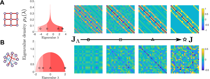
Figure 2: Dynamics of neurons on lattices versus networks can appear to differ substantially, depending on features like the statistics of synaptic connections between neurons and the signs of those synaptic connections. For example, A) shows the dynamics of a simulated network of excitatory neurons connected to their neighbors on a 2-dimensional lattice. Initially, the neurons fire asynchronously at intermediate rates. At $t=3333$ timesteps into the simulation, the gain of the neurons is increased (reflecting, for example, changes in attention of the organism), which creates two metastable states of high or low firing rate that drift through the network. In comparison, for the network of B) neurons are connected randomly with synaptic strengths of either sign; we set $J_{ii}=0$ for this example. Because there is not spatial organization, it is not clear if the increase in gain creates metastable states of activity in the network, or if it merely increases the variance of the network. Network models like this have been studied extensively using approximate techniques like mean-field theory, but understanding the roles that stochastic fluctuations play in these systems demands the use of tools from the renormalization group (RG).

Evaluating the frequency integrals and taking the infinite network limit $N\rightarrow\infty$, the flow equation for $U_{\Lambda}(\tilde{x},y)$ reduces to

$$\partial_{\Lambda}U_{\Lambda}(\tilde{x},y)=\frac{1}{2\tau}\rho_{\lambda}(\Lambda)\Bigg{\{}1-\Lambda U^{(1,1)}_{\Lambda}(\tilde{x},y)-\sqrt{\left(1-\Lambda U^{(1,1)}_{\Lambda}(\tilde{x},y)\right)^{2}-\Lambda^{2}U^{(0,2)}_{\Lambda}(\tilde{x},y)U^{(2,0)}_{\Lambda}(\tilde{x},y)}\Bigg{\}},$$ (14)

where $\rho_{\lambda}(\lambda)$ is the eigenvalue density, also known as the density of states when the synaptic connections form a nearest-neighbor lattice. An important result is that the flow equation is independent of the eigenvectors of $J_{ij}$. Thus, any networks with the same eigenvalue density and bare nonlinearity $\phi(y)$ will have the same effective firing rate nonlinearity within the local potential approximation. However, the statistics of the network activity will depend on the eigenvectors through the solution of the self-consistent equations $\nu_{i}=\Phi_{1}(\psi_{i}),~{}\psi_{i}=\mathcal{E}_{i}+\sum_{j}J_{ij}\nu_{j}$.

By construction, the initial condition of Eq. (14) is $U_{\Lambda=\Lambda_{\rm min}}(\tilde{x},y)=(e^{\tilde{x}}-1)\phi(y)$. The boundary conditions are a more subtle issue, and most papers on the NPRG method do not discuss them in depth. Common means of imposing boundary conditions are to i) compute derivatives at the boundaries of the numerical grid using only points internal to the grid DuclutPRE2017 , ii) impose that the solution matches the mean-field or 1-loop approximations at the numerical boundaries caillol2012non , or iii) expand the function in a power series around some point and truncating the series at some order, resulting in a reduced system of differential equations (however, the truncation is equivalent to implicitly imposing the missing boundary conditions robinson2003infinite ). In this work we focus on a combination of method iii with ii, as it is numerically the most tractable.

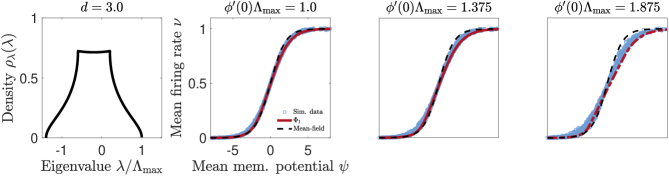
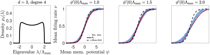
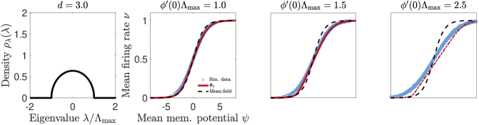
Figure 3: Effective nonlinearities on different networks with effective dimension $d=3$, along with their corresponding eigenvalue distributions $\rho_{\lambda}(\lambda)$ (far left). We show a $3$-dimensional hypercubic network (top), a random regular graph of degree $4$ (middle), and a Gaussian random network (bottom). For each network we show a subcritical nonlinearity (left), a near-critical nonlinearity (middle), and a supercritical nonlinearity (right), although the networks themselves are not critical because we use random distributions of resting potentials $\mathcal{E}_{i}$ to resolve the nonlinearities. Further examples for different effective dimensions $d$ are given in the Supplementary Information SuppInfo . The red curves are the predictions of the hierarchy of nonlinearities (Eqs. (15)), truncated at fourth order for subcritical and critical cases and first order for the supercritical case, using the results of loh2011accurate to compute the eigenvalue distributions. Blue data points are simulated data, using networks of $N=10^{3}$ neurons.

Expanding $U_{\Lambda}(\tilde{x},y)$ in a series around $\tilde{x}=0$ and truncating at a finite power $\tilde{x}^{m}$ yields an infinite hierarchy of of flow equations for the effective nonlinearities

$$\Phi_{m,\Lambda}(y)\equiv U_{\Lambda}^{(m,0)}(0,y)$$

for $m>0$. The rationale for expanding around $\tilde{x}=0$ is that this is the expected value of the membrane response field $\tilde{\psi}_{i}(t)=\langle\tilde{V}_{i}(t)\rangle$ when the network reaches a steady state. All of these nonlinearities share the initial condition $\Phi_{m,\Lambda_{\rm min}}(y)=\phi(y)$. Each equation in the hierarchy is coupled to the previous $m-1$ equations as well as the $(m+1)^{\rm th}$. That is, the hierarchy has the structure

$$\partial_{\Lambda}\Phi_{m,\Lambda}(y) =\mathcal{F}_{m}(\Phi_{1,\Lambda},\Phi_{2,\Lambda},\dots,\Phi_{m,\Lambda},\Phi_{m+1,\Lambda})$$ (15)

for each $m$, where the functions $\mathcal{F}_{m}$ depend on the nonlinearities as well as derivatives of those nonlinearities, which are not denoted explicitly as arguments.

Because each nonlinearity is coupled to the subsequent nonlinearity in the hierarchy, we need to approximately close the hierarchy at a finite order of $m$ to solve it. The simplest such approximation consists of setting the nonlinearities on the right hand side of Eqs. (15) to their initial values $\phi(y)$. However, this amounts to the one-loop approximation berges2002non , which breaks down when $1-\Lambda\phi^{\prime}(0)$ vanishes, and we do not expect it to perform better than the perturbative diagrammatic methods of OckerPloscb2017 ; KordovanArxiv2020 .

We instead truncate at order $m$ by approximating only $\Phi_{m+1,\Lambda}(y)\approx\phi(y)$. The singular factor is now $1-\Lambda\Phi^{\prime}_{1,\Lambda}(y)$, but renormalization of $\Phi^{\prime}_{1,\Lambda}(0)$ results in the solution persisting until we chose a $\Lambda_{\rm max}$ such that $1-\Lambda_{\rm max}\Phi^{\prime}_{1,\Lambda_{\rm max}}(0)=0$, corresponding to the phase transition. The solution continues beyond this value of $\Lambda_{\rm max}$, however, because the solution becomes non-analytic, out of the range of perturbative calculations. This singularity does cause problems for our numerical solution of the hierarchy, but we will show that we can still obtain a semi-quantitative solution and understand the supercritical behavior of the network qualitatively.

We show an explicit example of the truncation to second order in Eqs. (16)-(17), setting $\Phi_{3,\Lambda}(y)\approx\phi(y)$). In practice, for the subcritical results shown in this paper we truncate at order $4$, and for the supercritical results we truncate at order $1$.

$$\partial_{\Lambda}\Phi_{1,\Lambda}(y) =\frac{\rho_{\lambda}(\Lambda)\Lambda^{2}}{4\tau}\frac{\Phi_{2,\Lambda}(y)\Phi_{1,\Lambda}^{\prime\prime}(y)}{\left|1-\Lambda\Phi_{1,\Lambda}^{\prime}(y)\right|},$$ (16)

$$\partial_{\Lambda}\Phi_{2,\Lambda}(y) =\frac{\rho_{\lambda}(\Lambda)\Lambda^{2}}{8\tau}\left[\frac{\Lambda^{2}\Phi_{2,\Lambda}(y)^{2}\Phi_{1,\Lambda}^{\prime\prime}(y)^{2}}{|1-\Lambda\Phi_{1,\Lambda}^{\prime}(y)|^{3}}+\frac{4\Lambda\Phi_{2,\Lambda}(y)\Phi_{2,\Lambda}^{\prime}(y)\Phi_{1,\Lambda}^{\prime\prime}(y)}{|1-\Lambda\Phi_{1,\Lambda}^{\prime}(y)|^{2}}+\frac{4\phi(y)\Phi_{1,\Lambda}^{\prime\prime}(y)+2\Phi_{2,\Lambda}(y)\Phi_{2,\Lambda}^{\prime\prime}(y)}{|1-\Lambda\Phi_{1,\Lambda}^{\prime}(y)|}\right].$$ (17)

The initial initial conditions are $\Phi_{m,\Lambda_{\rm min}}(y)=\phi(y)$, with boundary conditions $\lim_{|y|\rightarrow\infty}\Phi_{m,\Lambda_{\rm min}}(y)\sim\phi(y)$ for $m=1,2$.

For sufficiently small $\Lambda_{\rm max}\phi^{\prime}(0)$ the denominator $1-\Lambda\Phi_{1,\Lambda}^{\prime}(y)$ remains positive for the duration of the flow, and the solution is analytic. However, at a critical value of $\Lambda_{\rm max}\phi^{\prime}(0)$ the denominator vanishes at the end of the flow, $1-\Lambda_{\rm max}\Phi_{1,\Lambda_{\rm max}}^{\prime}(0)=0$, corresponding to a critical point. Above this critical value of $\Lambda_{\rm max}\phi^{\prime}(0)$ the solution develops a range of $y$ for which $1-\Lambda\Phi_{1,\Lambda}^{\prime}(y)=0$, compensated by the second derivatives of the $\Phi_{m,\Lambda}^{\prime\prime}(y)$ vanishing on this range. This corresponds to a supercritical regime in which the solution is non-analytic, analogous to the development of the non-analyticity in the free-energy of the Ising model in the ordered phase GoldenfeldBook1992 .

We present results for three different types of networks with sigmoidal nonlinearity $\phi(V)\propto(1+e^{-V})^{-1}$ in Fig. 3: a $3d$ lattice of neurons with excitatory nearest-neighbor connections, a random regular graph of neurons with $4$ excitatory connections to randomly chosen targets, and a random network with Gaussian distributed synaptic weights. (We introduce heterogeneity into the rest potentials $\mathcal{E}_{i}$ for the excitatory networks, and set $\mathcal{E}_{i}=0$ for the Gaussian network, so that every neuron has a different steady state rate, which allows us to map out the effective nonlinearity $\Phi_{1}(\psi)$ by making a scatter plot of $\nu_{i}$ versus $\psi_{i}$).

In the subcritical regime the flow equations can be numerically integrated to predict the effective nonlinearity, and we have implemented this solution up to order 4 ($\Phi_{5,\Lambda}(y)\approx\phi(y)$). The solutions are reasonably good for $\Phi_{1,\Lambda}(y)$ and $\Phi_{2,\Lambda}(y)$ when truncated at this order, with $\Phi_{3,\Lambda}(y)$ exhibiting some influence of the truncation and $\Phi_{4,\Lambda}(y)$ suffering the most influence (not shown). In principle, truncating at higher orders should improve the numerical solutions further, though the flow equations become increasingly complicated. Our approximation does systematically undershoot the data near the negative tail of the distribution. It is unclear if this is an artifact of the local potential approximation, the hierarchy closure approximation, or finite-size effects in the simulations.

In the supercritical regime the numerical solution becomes increasingly challenging. The development of the non-analytic behavior is straightforwardly observed at the order $1$ approximation ($\Phi_{2,\Lambda}(y)\approx\phi(y)$). At higher orders it is difficult to coax Mathematica to integrate through the development of the non-analyticity, reminiscent of barriers integrating through the development of non-analytic shocks in nonlinear wave equations StackExchangeBurgers . Nevertheless, we obtain a qualitative picture of what happens in the supercritical regime: in order for the flow to be finite, the nonlinearity develops a piecewise linear region for $y\in[\psi_{-},\psi_{+}]$—where the endpoints of this region, $\psi_{\pm}$, depend on the initial value of $\phi^{\prime}(0)\Lambda_{\rm max}$—such that second order derivatives in the numerator vanish and cancel out the singularity caused by $1-\Lambda\Phi^{\prime}_{1}(y)=0$ in the denominator. Outside of this region $1-\Lambda\Phi^{\prime}_{1}(y)<0$ and the nonlinearity is smooth and continuous. We will use this semi-quantitative picture later when investigating the dynamics of the mean membrane potentials in the supercritical regime (Sec. II.1).

II.1 Phase transition analysis with effective nonlinearities

Now that we understand the qualitative behavior of the effective nonlinearities, we can revisit the phase transition analysis discussed in the context of mean-field theory in Sec. I.2. The conditions for a phase transition become

$$\mathcal{E}_{i}+\sum_{j}J_{ij}\Phi(0) =0,$$ (18)

$$\xi_{\tau}^{-1}/\tau^{-1}=1-\Lambda_{\rm max}\Phi^{\prime}(0) =0$$ (19)

as $N\rightarrow\infty$, where $\Phi(\psi)\equiv U^{(1,0)}_{\Lambda=\Lambda_{\rm max}}(0,\psi)$ is the effective nonlinearity, which we remind the reader determines the expected firing rates via the relation $\langle\dot{n}_{i}(t)\rangle=\Phi(\langle V_{i}(t)\rangle)$. The first condition just means that the mean input into a neuron is $0$, and hence $\langle V_{i}(t)\rangle=0$ self-consistently (as we inserted $\langle V_{i}(t)\rangle=0$ into $\Phi(\langle V_{j}(t)\rangle))$); in a heterogeneous network $\mathcal{E}_{i}$ can be set to a single value for all neurons to tune the population average of the membrane potential to $0$ SuppInfo , but we will not focus on this case explicitly. The second condition says that the largest relaxation time $\xi_{\tau}^{-1}$ of the network diverges, equivalent to the divergence of the temporal correlation length.

In the subcritical regime $1-\Lambda_{\rm max}\Phi^{\prime}_{1}(0)>0$, the mean-field analysis does not change, as $\Phi_{1}(\psi)$ is analytic, and so we expect an exponential decay to $\psi_{i}(t)=\langle V_{i}(t)\rangle=0$. Qualitatively, the critical case is not expected to change either, giving rise to an algebraic decay of $\psi_{i}(t)$. However, one generally expects the power of this decay to be modified at the critical point, as the leading order super-linear behavior of $\Phi_{1}(\psi)$ is expected to be non-analytic at the critical point. We cannot solve the flow equations with enough precision to try and predict this exponent quantitatively, but we revisit this exponent in the next section on universality.

Finally, the dynamics in the supercritical regime are much different than the mean-field analysis suggests, due to the development of the piecewise-linear region of $\Phi_{1}(\psi)$. The “extremal” values of the membrane potential, corresponding to the values of $\psi$ at which $\Phi_{1}(\psi)$ switches from the linear behavior to the nonlinear behavior, are fixed points of the membrane dynamics in a homogeneous excitatory network, and we typically would expect to observe the supercritical network to be in one of those states. These two states therefore represent two extremal metastable states of the network, analogous to the positive and negative magnetization phases of the Ising model.

The linear regime represents a line of metastable states. Homogeneous excitatory networks can be prepared to be in this metastable regime, though sudden perturbations can causet phase separation, as shown in Fig. 1A, which depicts simulations in which different local patches of neurons in a 2d lattice separate spatially into the metastable low firing-rate state or high firing rate state.

For symmetric random networks $J_{ij}$ with both excitatory and inhibitory connections, we expect the network to be in a spin glass regime. The population-distribution of the membrane potentials can be understood using the dynamical mean-field theory method for spin glasses sompolinsky1982relaxational applied to the dynamical equations for $\psi_{i}(t)$:

$$\tau\frac{d\psi_{i}(t)}{dt} =-\psi_{i}(t)+\sum_{j=1}^{N}J_{ij}\left(\Phi_{1}(\psi_{j}(t))-\Phi_{1}(0)\right),$$

where we set $\mathcal{E}_{i}=-\sum_{j}J_{ij}\Phi_{1}(0)$. The key difference between the standard dynamic mean-field calculations and our case is that the nonlinearity $\Phi_{1}(\psi)$ changes with the tuning parameter $\Lambda_{\rm max}$, whereas in previous treatments the nonlinearity is a fixed quantity. The dynamic mean-field calculation is not as tractable as it is in the case of asymmetric random networks with independent $J_{ij}$ and $J_{ji}$ kadmon2015transition ; schuecker2018optimal ; marti2018correlations ; stapmanns2020self , or the original spin-glass treatment of the Ising model sompolinsky1982relaxational . In particular, the non-analytic behavior of the effective nonlinearity $\Phi_{1}(\psi)$ in the critical and supercritical regimes renders the self-consistent equations difficult to solve analytically and elucidate how heterogeneous synaptic weights influence the critical properties we discuss in the next section. We discuss possible routes forward in the Discussion.

III Universality in the renormalization group flow

So far, our renormalization group (RG) treatment of the spiking network model has implemented the first step of an RG procedure, coarse-graining. This has allowed us to calculate non-universal features of the network statistics that hold regardless of whether the network is close to a phase transition. In this section we turn our attention to networks tuned to a phase transition, at which the statistics are expected to exhibit universal scale-invariant properties that can in principle be measured in experiments. To investigate these universal features, we must implement the second step of the RG procedure, rescaling. In the non-perturbative renormalziation group (NPRG) context, the rescaling procudure will amount to identifying an appropriate non-dimensionalization of the flow equation Eq. (14) and searching for fixed points.

This section proceeds as follows: we will first identify the rescaling of the NPRG flow equations that renders them dimensionless, and will admit fixed points. We will search for these fixed points using a combination of a perturbation expansion and non-perturbative truncations. This will show that the mean-field prediction of a second-order transition is qualitatively invalidated in spontaneous networks.

III.1 Non-dimensionalization of the flow equation

In translation-invariant lattices and continuous media, rescaling a theory is typically done by scaling variables and fields with powers of momentum; it is not a priori obvious how to perform this step for general networks. The resolution in this more general setting is that near a critical point quantities will scale as powers of $\delta\Lambda\equiv\Lambda_{\rm max}-\Lambda$.

To isolate the singular behavior of the RG flow as it approaches a critical point, it is convenient to define $U_{\Lambda}(\tilde{x},y)=\Lambda_{\rm max}^{-1}\tilde{x}y+W_{\Lambda}(\tilde{x},y)$, where $\Lambda_{\rm max}^{-1}$ is the critical value of $G_{11,\Lambda=\Lambda_{\rm max}}\equiv U_{\Lambda=\Lambda_{\rm max}}^{(1,1)}(0,0)$, such that $W^{(1,1)}_{\Lambda=\Lambda_{\rm max}}(0,0)=0$ at the critical point. We look for a scale invariant solution by making the change of variables $W_{\Lambda}(\tilde{x},y)=\Omega_{\Lambda}w_{s}(\tilde{z},z)$ with $\tilde{z}=\tilde{x}/\tilde{X}_{\Lambda}$ and $z=y/Y_{\Lambda}$, where $\Omega_{\Lambda}$, $\tilde{X}_{\Lambda}$, and $Y_{\Lambda}$ are running scales to be determined and $s=-\ln\left(\frac{\Lambda_{\rm max}-\Lambda}{\Lambda_{\rm max}-\Lambda_{\rm min}}\right)\in[0,\infty)$ is the “RG time” (which we define to be positive, in contrast to the convention in some NPRG works).

A straightforward way to determine the running scales $\Omega_{\Lambda}$, $\tilde{X}_{\Lambda}$, and $Y_{\Lambda}$ is to require the flow equation (14) to become asymptotically autonomous as $s\rightarrow\infty$. One can also find these scalings by rescaling the full average effective action (AEA), but it is more involved, and requires a careful consideration of the $N\rightarrow\infty$ limit in the eigenbasis of $J_{ij}$; we give this derivation in SuppInfo . In the scalings that follow below, we define the effective dimension $d$ by the scaling of the eigenvalue distribution near $\Lambda_{\rm max}$, $\rho_{\lambda}(\Lambda)\sim\delta\Lambda^{d/2-1}$. This definition is chosen so that the effective dimension is equal to the spatial dimension when $J_{ij}$ is a nearest-neighbor lattice with homogeneous coupling. Such a definition has previously been proposed in investigations of the $\phi^{4}$ theory on deterministic lattices tuncer2015spectral . With this definition, we find $\Omega_{\Lambda}\sim\delta\Lambda^{d/2+1}\sim e^{-s(d/2+1)}$ and the combination $\tilde{X}_{\Lambda}Y_{\Lambda}\sim\Omega_{\Lambda}/\delta\Lambda\sim\delta\Lambda^{d/2}$. Importantly, we can only constrain the combination $\tilde{X}_{\Lambda}Y_{\Lambda}$, which means that there is a “redundant parameter”, similar to the case in models with absorbing state transitions Janssen2004pair . This allows us to introduce a running exponent $\eta^{X}_{s}$ by defining $\tilde{X}_{\Lambda}\sim\delta\Lambda^{\eta^{X}_{s}}=e^{-s\eta^{X}_{s}}$ and $Y_{\Lambda}\sim\delta\Lambda^{d/2-\eta^{X}_{s}}=e^{-s(d/2-\eta^{X}_{s})}$. Note that this exponent does not arise from any field renormalizations, as our Ward-Takahashi identity guarantees no such field renormalizations exist. We will discuss the determination of $\tilde{X}_{\Lambda}$ shortly. First, we present the dimensionless flow equation, whose asymptotically autonomous form as $\delta\Lambda\rightarrow 0$ is

$$\partial_{s}w_{s}-\left(\frac{d}{2}+1\right)w_{s}+\eta^{X}_{s}\tilde{z}w_{s}^{(1,0)}+\left(\frac{d}{2}-\eta^{X}_{s}\right)zw_{s}^{(0,1)} =1-w_{s}^{(1,1)}-\sqrt{\left(1-w_{s}^{(1,1)}\right)^{2}-w^{(0,2)}_{s}w^{(2,0)}_{s}}.$$ (20)

Although Eq. (20) is only valid for RG-times $s\rightarrow\infty$, we retain some autonomous time-dependence for the purposes of performing linear stability analyses around fixed points of the flow. For the fully non-autonomous flow, see SuppInfo .

We will not solve Eq. (20) directly, as its numerical solution is rendered delicate by the divergence of $w_{s}$ when it is not near a critical manifold. This is in contrast to its dimensionful counterpart Eq. (14), which remains finite over the course of integration. To assess the critical properties of the model, we will focus on searching for fixed point solutions, using a combination of traditional perturbative techniques and additional functional truncations of $w_{\ast}(\tilde{z},z)$ to a finite number of couplings that can be treated non-perturbatively.

To find fixed point solutions, we need to make a choice of the running scale $\tilde{X}_{\Lambda}$. We briefly discuss the most natural choice $\tilde{X}_{\Lambda}=1$, and then focus on two choices corresponding to networks with absorbing states and spontaneously active networks.

III.2 Pure annihilation fixed point

The variable $\tilde{x}$, corresponding to the spike response fields $\tilde{\nu}_{i}(t)$, is dimensionless, appearing in the bare potential through $e^{\tilde{x}}-1$. Its “dimensionless” counterpart $\tilde{z}=\tilde{x}/\tilde{X}_{\Lambda}$ could therefore be chosen to be equal to $\tilde{x}$ itself by setting $\tilde{X}_{\Lambda}=1$. However, as we will see momentarily, the resulting fixed points $w_{\ast}(\tilde{z},z)$ are unstable to couplings in the model that cannot all be simultaneously tuned to put the RG flow on the stable manifold of these fixed points.

One fixed point is the trivial solution $w_{\ast}(\tilde{z},z)=0$. This is analogous to the Gaussian fixed point in most field theoretic RG studies. A linear stability analysis around the trivial fixed point reveals that perturbations to all couplings of order $z^{0}$ and $z^{1}$ are unstable (“relevant”) in any dimension $d$, independent of $\tilde{z}$. This means that in order to tune the network to this trivial critical point, one has to adjust entire functions of $\tilde{z}$ to some “critical functions.” For our initial condition $w_{0}(\tilde{z},z)$ these functions start at $(e^{\tilde{z}}-1)\phi(0)$ and $(e^{\tilde{z}}-1)\phi^{\prime}(0)z$, and it is not clear that the two parameters $\phi(0)$ and $\phi^{\prime}(0)$ are sufficient to tune the entire model to this critical point. We therefore expect that for effective dimensions $d>2$ any phase transitions are more likely to be controlled by some other fixed points, which we will find by using non-trivial choices of the running scale $\tilde{X}_{\Lambda}$.

III.3 Absorbing state networks

A commonly used class of nonlinearities in network models are “rectified units,” which vanish when the membrane potential is less than a particular value (here, $0$): $\phi(V)=0$ for $V\leq 0$. Neurons with rectified nonlinearities are guaranteed not to fire when their membrane potentials are negative, and as a result the network boasts an “absorbing state:” once the membrane potentials of all neurons drop below this threshold the network will remain silent. It is possible, in the $N\rightarrow\infty$ limit, that mutually excitatory neurons can maintain network activity at a high enough level that the network never falls into the absorbing state and remains active. Non-equilibrium models with absorbing states often fall into the directed percolation universality class janssen2005field , with exceptions when there are additional symmetries satisfied by the microscopic action tarpin2017nonperturbative .

The primary symmetry of the directed percolation (DP) universality class is the “rapidity symmetry.” Translated into the spiking network model, rapidity symmetry would correspond to an invariance of the average effective action under the transformation $\tilde{\nu}_{i}(t)\leftrightarrow-c\psi_{i}(t)$, where $c$ is a specific constant, chosen so that the terms $\tilde{\nu}_{i}(t)\psi_{i}(t)^{2}$ and $\tilde{\nu}_{i}(t)^{2}\psi_{i}(t)$ transform into each other (including their coefficients). The spiking network does not obey this symmetry; however, most models in the DP universality class do not exhibit rapidity symmetry exactly, and it is instead an emergent symmetry that satisfied after discarding irrelevant terms in an action tuned to the critical point henkel2008universality . We will show this is true for the absorbing state spiking network.

The spiking network action does not appear to admit any obvious symmetries beyond the the Ward-Takahashi identities. One of the consequences of these identities is the prediction that the dynamic exponent is $z_{\ast}=2$, unmodified from its “mean-field” value. A trivial dynamic exponent is also a feature of the “directed percolation with coupling to a conserved quantity” (DP-C) universality class janssen2005field , which is another possible candidate for the universality class of the spiking network. The DP-C class has a symmetry that also predicts a correlation length exponent of $\nu_{\ast}=2/d$, which is not guaranteed by our Ward-Takahashi identities but could be an emergent property if the model is in the DP-C class. (Note that we will give critical exponent symbols $*$ subscripts to distinguish them from the variables $z$ and field $\nu$). To demonstrate that the spiking network model supports a DP-like critical point, we will choose the running scale $\tilde{X}_{\Lambda}$ to impose the rapidity symmetry relationship on the lowest order couplings. We assume that $\phi^{\prime}(0^{+})>0$ and $\phi^{\prime\prime}(0^{+})<0$, and choose $\tilde{X}_{\Lambda}=Y_{\Lambda}|W_{\Lambda}^{(1,2)}(0,0)|/W_{\Lambda}^{(2,1)}(0,0)$. This renders $g_{21,s}=-g_{12,s}$ for all $s$, a hallmark of the Reggeon field theory action that describes the directed percolation universality class janssen2005field ; canet2006reaction . We can then show that $w_{\ast}(\tilde{z},z)=0,~{}\eta^{X}_{\ast}=d/4$ is a trivial fixed point for which the combination of terms $\tilde{z}z^{2}-\tilde{z}^{2}z$ loses stability below the upper critical dimension $d_{c}=4$.

The exponent $\eta^{X}_{s}$ can be defined by differentiating Eq. (20) to derive equations for $g_{12,s}$ and $-g_{21,s}$ and equating them. This reveals that

$$\eta^{X}_{s} =\frac{d}{4}+\frac{1}{2}\frac{g_{13,s}-g_{31,s}}{1-g_{11,s}}.$$ (21)

In general, rapidity symmetry requires $g_{mn}^{\ast}=(-1)^{m+n}g_{nm}^{\ast}$ canet2006reaction . Under this assumption, $\eta^{X}_{\ast}=d/4$ for all $d$ and the anomalous exponent $\delta\eta^{X}_{\ast}=\eta^{X}_{\ast}-d/4$ is always $0$.

To capture the key features of the RG flow, we expand the running potential in a power series,

$$w_{s}(\tilde{z},z) =\sum_{m,n=1}^{\infty}\frac{g_{mn,s}}{m!n!}\tilde{z}^{m}z^{n},$$

truncating at some finite order in $\tilde{z}$ and $z$. This truncation does not reflect an assumption that the variables are small, but a further projection onto a reduced solution subspace, similar to analyses of, e.g., the Ising model, that track only the flow of two couplings despite coarse graining generating couplings of all orders. To close the equations, a system of differential equations is obtained by differentiating Eq. (20) with respect to the appropriate powers of $\tilde{z}$ and $z$ and evaluating at $(\tilde{z},z)=(0,0)$. In this expansion we have $g_{12,s}=-g_{21,s}$ by construction, but we need not impose the rapidity symmetry on the higher order terms, so that we may check how the lack of this symmetry at the dimensionful level affects the RG flow. Note that because rapidity symmetry imposes a relationship between $g_{mn}^{\ast}$ and $g_{nm}^{\ast}$, any truncation we make must include both terms.

III.3.1 Minimal truncation

The RG flow in the $g_{11}{-}g_{21}$ plane is shown in Fig. 4. We find that the upper critical dimension is $4$: in $d>4$ only the trivial fixed point $(g_{11}^{\ast},g_{21}^{\ast})=(0,0),~{}\eta^{X}_{\ast}=d/4$ exists, while in $d<4$ we find fixed point solution for the minimal truncation is

$$\eta^{X}_{\ast}=\frac{d}{4},~{}g_{11}^{\ast}=\frac{4-d}{12-d},~{}g_{21}^{\ast}=\frac{4\sqrt{4-d}}{\sqrt{d^{2}-24d+144}},$$

with $g_{12}^{\ast}=-g_{21}^{\ast}$. From this solution we see that the fixed point values of the couplings scale as powers of $\sqrt{4-d}$. This suggests that if we set $\epsilon=4-d$ our series expansion should be in powers of $\sqrt{\epsilon}$.

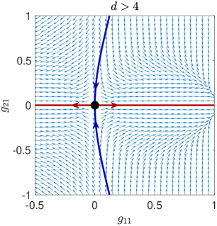
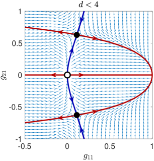
Figure 4: Renormalization group flow of the absorbing state network model in the space of the couplings $g_{11}$ and $g_{21}$, for effective dimensions $d>4$ and $d<4$, where $4$ is the upper critical dimension. In $d>4$ only a trivial fixed point exists, while in $d<4$ two equivalent fixed points exist, only one of which is selected by the initial conditions of the network model. The stable and unstable manifolds (solid lines) are colored according to the critical points (saddle nodes), with blue indicating the stable manifold and red indicating unstable manifolds.

By performing a linear stability analysis around the trivial and non-trivial fixed points we can estimate the correlation length exponent $\nu_{\ast}$ from the largest eigenvalue of the stability matrix, $\mu$: $\nu_{\ast}=(2\mu)^{-1}$. (The factor of $1/2$ is included so that the value of $\nu_{\ast}$ matches the numerical values obtained in prior work in translation invariant systems. We also retain the name “correlation length exponent,” even though there may not be a notion of spatial distance in arbitrary networks). When $d>4$ the trivial fixed point has one negative and one positive eigenvalue, signaling the fact we must tune only one parameter to arrive at this fixed point. The positive eigenvalue at the trivial fixed point is $\mu=1$ in $d>4$, giving $\nu_{\ast}=1/2$, as expected. In $d<4$ the trivial fixed point becomes wholly unstable as it splits into the pair of non-trivial fixed points shown in Fig. 4, which each have a stable and unstable direction, and the eigenvalue of the flow along the unstable manifold gives the correlation length exponent, which for $d\rightarrow 4^{-}$ is $\nu_{\ast}\approx 1/2+(4-d)/16-7/128(4-d)^{2}+\dots.$ Although $g_{21}^{\ast}$ scales as $\sqrt{4-d}$, the lowest order dependence of $\nu_{\ast}$ is linear. The expansion of $\nu_{\ast}$ near $d=4^{-}$ matches the one-loop approximation of $\nu_{\ast}$ for Reggeon field theory, the first suggestion that the spiking network is more like the standard DP class, not the DP-C class, for which $\nu_{\ast}=2/d\approx 1/2+(4-d)/8+\dots$ janssen2005field .

Although within this minimal truncation we obtain an expression for $\nu_{\ast}$ valid for all $d<4$, the result begins decreasing non-monotonically as $d$ is lowered below $\sim 3.2$. This non-monotonic behavior is an artifact of the truncation, as we will show by increasing the truncation order. To facilitate our higher order truncations we first turn to a perturbative expansion.

III.3.2 Perturbative fixed point solution in powers of $\sqrt{4-d}$

One can implement the so-called “$\epsilon$-expansion” in the NPRG framework by assuming the fixed point solution $w_{\ast}(\tilde{z},z)$ can be expanded in a series of powers of the distance from the upper critical dimension $d_{c}$, $\epsilon\equiv d_{c}-d$. As our minimal truncation showed, however, we expect some of the couplings to depend on $\sqrt{\epsilon}$, which we will use as our expansion parameter:

$$w_{\ast}(\tilde{z},z) =\epsilon^{1/2}w_{1}(\tilde{z},z)+\epsilon w_{2}(\tilde{z},z)$$

$$~{}~{}~{}~{}~{}+\epsilon^{3/2}w_{3}(\tilde{z},z)+\epsilon^{2}w_{4}(\tilde{z},z)+\dots$$ (22)

$$\eta^{X}_{\ast} =1+\epsilon^{1/2}\delta\eta_{1}+\epsilon\delta\eta_{2}+\epsilon^{3/2}\delta\eta_{3}+\epsilon^{2}\delta\eta_{4}+\dots.$$ (23)

Because the trivial fixed point is $w_{\ast}(\tilde{z},z)=0$, there are no $\epsilon^{0}$ terms. For this calculation we will not assume $\eta^{X}_{\ast}=d/4=1-\epsilon/4$ at the outset, to allow for the possibility of discovering a solution that does not obey rapidity symmetry, though it turns out there is no such solution perturbatively.

We insert the expansions (22)-(23) into Eq. (20) and expand in powers of $\epsilon^{1/2}$, resulting in a hierarchy of linear equations whose solutions depend on the previous solutions in the hierarchy. A valid critical point solution must exist for all $\tilde{z}$ and $z$, so we fix constants of integration and the coefficients of $\eta^{X}_{\ast}$ order by order to eliminate terms that are not polynomially bounded in $z$. The result to $\mathcal{O}(\epsilon^{2})$ is

$$w_{\ast}(\tilde{z},z) =2a\frac{\tilde{z}^{2}z-\tilde{z}z^{2}}{2!}\epsilon^{1/2}+2a^{2}\tilde{z}z\epsilon-\frac{544a^{5}}{48a^{2}-1}\frac{\tilde{z}^{2}z-\tilde{z}z^{2}}{2!}\epsilon^{3/2}$$

$$~{}~{}~{}~{}~{}~{}~{}~{}+\left(\left(\frac{1088a^{6}}{48a^{2}-1}+4a^{4}\right)\tilde{z}z+72a^{4}\frac{\tilde{z}^{2}z^{2}}{2!2!}-48a^{4}\frac{\tilde{z}^{3}z+\tilde{z}z^{3}}{3!}\right)\epsilon^{2}+\mathcal{O}(\epsilon^{5/2}),$$ (24)

where $a=0,\pm 1/4$. The first choice of $a$ corresponds to the trivial solution, while the second corresponds to two equivalent non-trivial solutions; we take the positive value $a=1/4$ to match the sign of our initial condition. We see that at order $\epsilon^{2}$ the combination $\tilde{z}^{3}z+\tilde{z}z^{3}$ appears, which obeys the expected rapidity symmetry. The exponent is $\eta^{X}_{\ast}=1-\epsilon/4+\mathcal{O}(\epsilon^{5/2}),$ which is just the exact result $\eta^{X}_{\ast}=d/4$.

We can estimate the linear stability of the solution by the standard method of perturbing $w_{s}(\tilde{z},z)=w_{\ast}(\tilde{z},z)+e^{\mu s}\delta w(\tilde{z},z)$, and expanding $\mu=\mu_{0}+\epsilon^{1/2}\mu_{1}+\epsilon\mu_{2}+\dots$, choosing $\mu_{0}$ to correspond to the eigenvalue of the largest allowed eigenvalue to zeroth order, and the remaining terms to non-polynomial divergent terms at large $z$. In this analysis we will assume rapidity symmetry to hold, such that we may fix $\eta^{X}_{\ast}=d/4$. In our higher-order non-perturbative analysis we will relax this assumption. We find that the largest eigenvalue of this fixed point gives a correlation length exponent of

$$\nu_{\ast}(\epsilon)=\frac{1}{2}+\frac{\epsilon}{16}+\frac{7}{256}\epsilon^{2}+\mathcal{O}(\epsilon^{3}).$$ (25)

To first order this agrees with both our minimal truncation and the epsilon expansion for the Reggeon field theory. The second order correction is numerically close to the 2-loop expansion for the Reggeon field theory, but is not the same. The discrepancy could be an artifact of our sharp regulator or our local potential approximation. Our result suggests that the universality class of this fixed point is more consistent with the regular DP class, rather than the DP-C class. However, it remains that our Ward-Takahashi identities predict a dynamic exponent of $z_{\ast}=2$ for all effective dimensions $d$, in contrast with the perturbative results for the Reggeon field theory. In the Discussion we explain that this trivial dynamic exponent is likely due to the linear membrane potential dynamics, and nonlinearities would contribute to an anomalous value of $z_{\ast}$, in which case the absorbing state fixed point may conform to the well-known DP class.

III.3.3 Non-perturbative truncation up to order $\tilde{z}^{5}z^{5}$

Because the $\epsilon$-expansion is expected to be exact close to $d=4^{-}$, we can use the results of our perturbative calculation as initial guesses in a numerical root-finding scheme in a higher order non-perturbative truncation. Once the roots are found numerically, we can decrease the value of $d$ and use the previously obtained numerical root as the initial guess for the root finder. We proceed iteratively in this way, allowing us to continuously track the non-trivial fixed point as we decrease $d$ from $4$, avoiding the erroneous roots introduced by our truncation.

We have performed our truncation up to order $\tilde{z}^{5}z^{5}$, beyond which the calculations become computationally expensive. We indeed still find a non-trivial fixed point with rapidity symmetry, for which we estimate the critical exponent $\nu_{\ast}$ by analyzing the eigenvalues of the flow. We insert the expression Eq. (21) for $\eta^{X}_{s}$ into the flow equations before linearizing, such that we can verify that the fixed point with rapidity symmetry is not unstable to some other fixed point lacking that symmetry, at least for some finite range of $d<4$. We indeed find that the DP fixed point has a single relevant direction for $2.78\lesssim d<4$. As $d\rightarrow 2.78^{+}$ the estimates for $\nu_{\ast}$ diverge for our $\tilde{z}^{3}z^{3}$ and $\tilde{z}^{4}z^{4}$ truncations, and cannot be continued for lower $d$ for our $\tilde{z}^{5}z^{5}$ truncation, as shown in Fig. 5. Interestingly, the estimate of $\nu_{\ast}$ in the $\tilde{z}^{5}z^{5}$ truncation appears to be quite close to the $\epsilon$-expansion up to the dimension where the solution ends. The restriction of this range indeed appears to be due to the development of an additional positive eigenvalue for $d\lesssim 2.78$, indicating the DP-like fixed point may become unstable to some other fixed point in this regime. However, numerical attempts to find this other fixed point suggest it may be the case that the second largest eigenvalue merely becomes small and close to zero, remaining so as $d$ is lowered further, which could just be an artifact of the approximation. We leave a detailed investigation of what happens in $d<2.78$ for future studies.

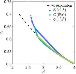
Figure 5: Correlation length exponent for the absorbing state network as a function of the effective dimension $d$. Obtained using the third (dark blue triangles), fourth (light blue circles), and fifth order (green squares) truncations. The estimates are compared to Eq. (25), the perturbative $\epsilon$-expansion estimate (black dashed line). The non-perturbative analysis suggests the fixed point becomes unstable toward another fixed point in $d\lesssim 2.78$.

III.4 Spontaneous networks

We now consider the case of spontaneously active networks, for which $\phi(0)\neq 0$. The probability of firing a spike is never $0$ at any finite $V$, so there is no absorbing state in this network. Instead, we anticipate that the network may be able to achieve active steady-states.

The fact that there is a membrane potential-independent component of the fluctuations in the spontaneous networks suggests we should choose the running scale $\tilde{X}_{\Lambda}=\sqrt{\Omega_{\Lambda}/W^{(2,0)}_{\Lambda}(0,0)}$. This choice renders $g_{20,s}=w_{s}^{(2,0)}(0,0)=1$ for all $s$, which is in essence like choosing the Gaussian part of the action to be invariant under the RG procedure. This restriction puts a constraint on the exponent $\eta^{X}_{s}$ in terms of the couplings $g_{mn,s}$:

$$\eta^{X}_{s} =\frac{d+2}{4}+\frac{1}{4}\frac{g_{22,s}+2g_{12,s}g_{30,s}}{1-g_{11,s}}$$

$$~{}~{}~{}~{}+\frac{1}{2}\frac{g_{12,s}g_{21,s}}{\left(1-g_{11,s}\right)^{2}}+\frac{1}{8}\frac{g_{12,s}^{2}}{\left(1-g_{11,s}\right)^{3}}$$ (26)

The reader can check that $w_{\ast}(\tilde{z},z)=\tilde{z}^{2}/2,~{}\eta^{X}_{\ast}=\frac{d+2}{4}$ is a trivial fixed point solution. A linear stability analysis of this fixed point shows that the couplings $g_{10,s}$ and $g_{11,s}$ are unstable SuppInfo . The divergent flow of $g_{10,s}$ does not contribute to any other coupling, only to the renormalized value of $\Phi_{1}(0)$, which is compensated by tuning the rest potentials $\mathcal{E}_{i}$. The flow of $g_{11,s}$ is the key relevant term; its initial value $g_{11,0}$ must be tuned so that the RG flow takes the model to the critical point.

A linear stability analysis of the trivial fixed point predicts that as the effective dimension $d$ is lowered the couplings $g_{1n,s}$ become relevant sequentially, with $g_{12}$ becoming relevant at $d=6$, then $g_{13}$ at $d=4$, and so on until all couplings are relevant in $d=2$. This is the standard sequence predicted for scalar field theories, like $\phi^{4}$ theory with symmetry breaking terms. The coefficients $g_{mn,s}$ with $m\geq 2,~{}n\geq 1$ are all irrelevant in $d>2$ SuppInfo .

In our exemplar case in the mean-field analysis explored in Sec. I.2, we chose a bare nonlinearity $\phi(V)=(1+\exp(-V))^{-1}$, which has $\phi^{\prime\prime}(0)=0$. Naively, then, it appears that $g_{12,0}=0$, and we might expect to find a Wilson-Fisher fixed point in $d<4$ related to the Ising universality class. While our dimensionless flow equations do admit such a fixed point solution, the $\mathbb{Z}_{2}$ symmetry of this fixed point is not a symmetry of the initial action for this model. Such a symmetry would manifest as an invariance to the transformation $w_{s}(\tilde{z},z)=w_{s}(-\tilde{z},-z)$, which the initial condition—a scaled version of $(e^{\tilde{x}}-1)\phi(V)-\phi(0)\tilde{x}$—does not satisfy. Thus, even though $g_{12,s}=0$ initially, we expect this term to be generated by the RG flow, and the mean-field prediction for this case will be qualitatively invalidated.

III.4.1 Minimal truncation

We validate our above claims by making a minimal truncation of $w_{\ast}(\tilde{z},z)=\tilde{z}^{2}/2+\tilde{z}(g_{11,s}z+g_{12,s}z^{2}/2+g_{13,s}z^{3}/3!)$. As expected, we find three valid fixed points: a trivial fixed point, a fixed point with a $\mathbb{Z}_{2}$ symmetry, and a third fixed point for which $g_{12}^{\ast}\neq 0$. Analysis of the eigenvalues of these three fixed points reveals that this third fixed point controls the RG flow below $d=6$, so we focus on its properties here.

The third fixed point is rather unwieldy in its exact form, so we instead give its behavior near the dimension $d=6$, where it coincides with the trivial solution:

$$g_{11}^{\ast} =\frac{6-d}{9}+\frac{(6-d)^{2}}{81}+\dots$$ (27)

$$g_{12}^{\ast} =\pm i\frac{\sqrt{2}}{3}\sqrt{6-d}\mp i\frac{5}{27\sqrt{2}}(6-d)^{3/2}+\dots$$ (28)

$$g_{13}^{\ast} =\frac{4}{27}(6-d)^{2}+\dots$$ (29)

$$\eta^{X}_{\ast} =2-\frac{5}{18}(6-d)-\frac{2}{81}(6-d)^{2}+\dots.$$ (30)

The most striking feature of this fixed point solution is that the coupling $g_{12}^{\ast}$ is imaginary. This is not an artifact of the truncation, but a signature of a spinodal point in the model, as observed in the critical $\phi^{3}$ theory. Indeed, zhong2012imaginary ; zhong2017renormalization argue that imaginary fixed points correspond to spinodal points associated with first order transitions, yet still possess several features of continuous transitions, such as universal critical exponents. i.e., the imaginary couplings have real physical consequences. Importantly, the anomalous exponents and correlation length exponent $\nu_{\ast}$ are purely real. We can visualize the flow of the couplings in the $g_{11}{-}g_{12}$ plane, shown in Fig. 6 (for this visualization we use a further truncation in which we set $g_{13}=0$, so that the flow is wholly two-dimensional). In Fig. 6A we show the flow for real-valued $g_{12}$, which reveals that in $d>6$ the trivial fixed point is the critical point, but two other unstable fixed points exist that collide with the trivial fixed point at $d=6$, leaving an unstable node with no other apparent fixed points in $d<6$. If we look at the flow for imaginary $g_{12}\rightarrow ig_{12}$, shown in Fig. 6B, we see that in $d>6$ only the trivial fixed point exists, and in $d<6$ it splits into two critical points that control the flow of the model. Notably, the flow in this plane looks like a regular RG flow — there is no exotic behavior such as limit cycles or spirals, which is a reflection of the fact that the critical exponents we will calculate below are purely real. If we could visualize the RG flow in the space complex $g_{12}$, what we would expect to see is a pair of purely real unstable fixed point values of $g_{12}$ in $d>6$, which exchange stability with the trivial fixed point at the upper critical dimension $d=6$, and become a pair of purely imaginary fixed points that control the critical behavior in $d<6$.

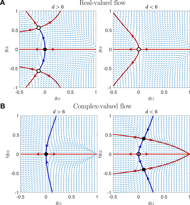
Figure 6: Renormalization group flow of the spontaneous network model in the space of the couplings $g_{11}$ and $g_{12}$, for effective dimensions $d>6$ and $d<6$, where $6$ is the upper critical dimension. A) For real-valued $g_{12}$, in $d>6$ the trivial fixed point coexists with two unstable fixed that merge with the trivial fixed point at $d=6$, leaving only an unstable node in $d<6$. B) For imaginary-valued $g_{12}\rightarrow ig_{12}$ only the trivial fixed point exists in $d>6$, splitting off into two non-trivial critical points in $d<6$. The stable and unstable manifolds (solid lines) are colored according to the critical points (saddle nodes), with blue indicating the stable manifold and red indicating unstable manifolds.

We confirm this picture by estimating the eigenvalues of the fixed points via a linear stability analysis. The analysis shows that $g_{11}$ is relevant in all dimensions, while $g_{12}$ and $g_{13}$ become relevant in $d=6$ and $d=4$, respectively. Numerical evaluation of the eigenvalues confirms that the complex spinodal critical point has two unstable directions in $d>6$ and one unstable direction for $d<6$, indicating that it is the controlling critical point for the spiking network model, even for dimensions $d<4$.

We will verify that higher order truncations give a consistent qualitative picture that agrees with the above analysis. To assist in this endeavor, we first derive the fixed point solution using an $\epsilon$-expansion.

III.4.2 Perturbative fixed point solution in powers of $\sqrt{6-d}$

The $\epsilon$-expansion proceeds similarly to the absorbing state network. We expand

$$w_{\ast}(\tilde{z},z) =\frac{\tilde{z}^{2}}{2}+\epsilon^{1/2}w_{1}(\tilde{z},z)+\epsilon w_{2}(\tilde{z},z)$$

$$~{}~{}~{}~{}+\epsilon^{3/2}w_{3}(\tilde{z},z)+\epsilon^{2}w_{4}(\tilde{z},z)+\dots$$

$$\eta^{X}_{\ast} =2+\epsilon^{1/2}\delta\eta_{1}+\epsilon\delta\eta_{2}+\epsilon^{3/2}\delta\eta_{3}+\epsilon^{2}\delta\eta_{4}+\dots$$

and insert this expansion into Eq. (20), deriving a hierarchy of linear equations. Demanding that the solutions are polynomially bounded as $z$ grows large yields the trivial solution as well as two equivalent non-trivial complex fixed points:

$$w_{\ast}(\tilde{z},z) =\frac{\tilde{z}^{2}}{2}+\frac{i}{12\sqrt{2}}\tilde{z}\left(4z^{2}-2\right)\epsilon^{1/2}+\frac{\tilde{z}z}{9}\epsilon$$

$$~{}~{}~{}~{}~{}-\frac{i}{216\sqrt{2}}\tilde{z}\left(\tilde{z}^{2}+12\tilde{z}z+16z^{2}+4\left(2z^{2}-1\right)\left(-2+\psi^{(0)}\left(-\frac{1}{2}\right)-\psi^{(0)}\left(\frac{1}{2}\right)\right)\right)\epsilon^{3/2}$$

$$~{}~{}~{}~{}+\Bigg{[}\frac{1}{162}\tilde{z}\left(z^{2}-\frac{1}{2}\right)\left(z\left(4z^{2}+19\right)-\left(8z^{4}+26z^{2}+19\right)F(z)\right)$$

$$~{}~{}~{}~{}+\frac{1}{324}\tilde{z}\left(\left(2z^{2}-1\right)F(z)-z\right)\left(8z^{4}+2z^{2}\left(5+4\psi^{(0)}\left(-\frac{1}{2}\right)-4\psi^{(0)}\left(\frac{1}{2}\right)\right)+11-4\psi^{(0)}\left(\frac{1}{2}\right)+4\psi^{(0)}\left(-\frac{1}{2}\right)\right)$$

$$~{}~{}~{}~{}+\frac{\tilde{z}^{2}z^{2}}{54}+\frac{5\tilde{z}^{3}z}{972}+\frac{5\tilde{z}^{4}}{10368}\Bigg{]}\epsilon^{2},$$ (31)

where $\psi^{(0)}\left(\cdot\right)$ is the Poly-Gamma function ($\psi^{(0)}\left(-1/2\right)\approx 0.03649$, $\psi^{(0)}\left(1/2\right)\approx-1.96351$) and $F(z)=\frac{\sqrt{\pi}}{2}e^{-z^{2}/2}{\rm erfi}(z)$ is the Dawson F function with ${\rm erfi}(z)=\frac{2}{\sqrt{\pi}}\int_{0}^{z}dt~{}e^{+t^{2}}$ the “imaginary error function.” The second non-trivial solution is the complex conjugate. As in the minimal truncation, the exponents turn out to be purely real. The anomalous exponent is

$$\delta\eta^{X}_{\ast} \equiv\eta^{X}_{\ast}-\frac{d+2}{4}=-\frac{1}{36}\epsilon+\frac{29}{648}\epsilon^{2}+\mathcal{O}(\epsilon^{5/2}).$$

We may attempt a linear stability analysis to estimate the critical exponent $\nu_{\ast}$, but the standard approach of perturbing $w_{s}(\tilde{z},z)=w_{\ast}(\tilde{z},z)+e^{\mu s}\delta w(\tilde{z},z)$ is complicated by the fact that $\eta^{X}_{s}$ flows near this fixed point and should be perturbed as well. Nonetheless, we calculate a rough estimate by fixing $\eta^{X}_{s}$ to its fixed point value, which we will find agrees with our other estimates to at least $\mathcal{O}(\epsilon^{3/2})$. We find that the correlation exponent $\nu_{\ast}$ is

$$\nu_{\ast}=\frac{1}{2}+\frac{\epsilon}{9}+\mathcal{O}(\epsilon^{2}).$$ (32)

Only the non-analytic powers of $\epsilon$ give rise to imaginary terms, consistent with the minimal truncation finding that this fixed point is purely real in $d>6$. It also turns out the real component of $\varphi_{1\ast}(z)$ is odd in $z$, while the imaginary components are even in $z$.

The fact that the critical point is complex implies the following behavior as one translates from the dimensionless flow to the dimensioned flow: when starting from real-valued initial conditions, the dimensionless flow equation will eventually blow up at a finite scale of the RG flow, but this divergence can be analytically continued into the complex plane, such that the flow is able to arrive at the critical point (for a fine-tuned initial condition). If the initial condition is complex to begin with, we expect a smooth flow to the critical point, as was shown for a toy model in zhong2012imaginary .

III.4.3 Higher order truncations

We now return to the non-perturbative truncations of the flow equations, using the perturbative results as seeds for the initial guess of a root finding algorithm near $d=6^{-}$. Unlike the absorbing state network, we do not have to truncate symmetrically in $\tilde{z}$ and $z$. The simplest truncation consists of setting $g_{mn,s}=0$ for all $m\geq 2,~{}n\geq 1$, and truncating $g_{mn,s}$ at a finite value of $n$. We show this truncation up to $n=7$ in Fig. 7; the numerical solution becomes increasingly difficult at larger orders.

The estimate of the anomalous exponent $\delta\eta^{X}_{\ast}$, shown in Fig. 7A, is determined entirely by the fixed point values of the couplings. The non-perturbatively computed values of $\delta\eta^{X}_{\ast}$ are entirely negative as a function of dimension; the $\epsilon$-expansion is also negative close to the upper critical dimension, but becomes positive for lower dimensions. Our results compare favorably to an NPRG study of the Yang-Lee $\phi^{3}$ theory of An et al. in Ref. an2016functional , providing numerical evidence that the spontaneous network fixed point may be in a closely related universality class.

Our estimates of the correlation length exponent $\nu_{\ast}$, computed using the linearized flow of the truncated equations around the fixed point, as opposed to exponent relations, are shown in Fig. 7B. We find consistent behavior as we increase $n$, but the estimates display a non-monotonic behavior that is likely an artifact of the truncation. Including higher order powers of $\tilde{z}$ in our truncation does not improve the result. We find that when $d<5$ the numerical estimates of the eigenvalues abruptly develop non-negligible imaginary components, jumping from $\mathcal{O}(10^{-17}{\sim}10^{-15})$ to $\mathcal{O}(10^{-4}{\sim}1)$, which is most likely an artifact of the truncation or numerical evaluation, and not a real emergence of complex eigenvalues in the RG flow.

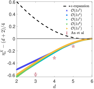
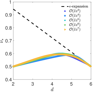
Figure 7: Anomalous and correlation length exponent estimates for the spinodal fixed point as a function of the effective dimension $d$. Top panel: Estimate of the anomalous exponent $\eta^{X}_{\ast}-(d+2)/4$ obtained at the non-trivial fixed point found for $2<d<6$, compared to the anomalous exponent estimates of Ref. an2016functional in the equilibrium Lee-Yang $\phi^{3}$ theory. Bottom panel: Estimates of the correlation length exponents $\nu_{\ast}$ obtained from the flow of the model near the fixed point, rather than expected exponent relations. We show results using truncations at linear order in $\tilde{z}$ and up to order $z^{7}$. The numerical estimates are compared to the perturbative $\epsilon$-expansion estimate (black dashed line), which is only expected to be reliable close to $d=6$. The non-perturbative analysis suggests the results may be reliable for $d\gtrsim 5$, but may require a more refined approximation than the local potential approximation in lower dimensions.

The non-monotonic estimates of $\nu_{\ast}$ below $d\approx 5$ could be a consequence of the local potential approximation. Ref. an2016functional ’s NPRG study of the spinodal point in the Yang-Lee model $\phi^{3}$ theory found that the local potential approximation alone was insufficient to find fixed points below $d\approx 5.6$, and a non-local ansatz like the derivative expansion is necessary to proceed. While the structure of the spiking network model differs in several important ways, it could be that to fully capture the behavior of the critical exponents as a function of dimension we need to generalize the derivative expansion to the present case. There are technical obstacles to doing so morris1998properties , so we leave this as a direction for future work.

III.5 Singular contributions to the firing rate nonlinearity at criticality

We end our current investigation of universality in the spiking network model by discussing the non-analytic contributions to the effective firing rate nonlinearity $\Phi_{1}(\psi)$. The critical effective firing rate nonlinearity is related to its dimensionless counterpart $\varphi_{1,\ast}(z)=w_{\ast}^{(1,0)}(0,z)$ via

$$\Phi_{1}(\psi) =\Phi_{1}(0)+\Lambda_{\rm max}^{-1}\psi$$

$$~{}~{}~{}~{}+\lim_{s\rightarrow\infty}e^{-s(d/2+1-\eta^{X}_{s})}\varphi_{1\ast}\left(\psi e^{s(d/2-\eta^{X}_{\ast})}\right)$$

$$~{}~{}~{}~{}+{\rm analytic~{}\&~{}subleading~{}singular~{}terms}.$$ (33)

The analytic terms arise from deviations of $\varphi_{1s}(z)$ away from the critical point, such as irrelevant couplings that are non-zero in the bare nonlinearity $\phi(V)$. We expect such terms to be higher order than the singular term, which would lead to the non-mean-field scaling behavior. The critical $\varphi_{1\ast}(z)$ gives rise to the singular non-analytic behavior that emerges at the critical point, which is in principle observable when the network is tuned to the critical point, though the analytic terms can make it difficult to measure the singular behavior, even if the system is close to a critical point. In homogeneous networks this singular behavior can be detected through power-law behavior of other quantities, while in heterogeneous networks, such as those with random $J_{ij}$, the singularity may be further masked by the effect of the disorder. Because the effective firing rate nonlinearity $\Phi_{1}(\psi)$ must be real and finite, $\varphi_{1,\ast}(z)$ must behave as a power-law for large $z$, such that the dependence on $s$ in Eq. (33) cancels out WinklerPRE2013 . This yields

$${\rm Re}[\Phi_{1}(\psi)-\Phi_{1}(0)-\psi/\Lambda_{\rm max}]$$

$$=\lim_{s\rightarrow\infty}e^{-s(d/2+1-\eta^{X}_{\ast})}{\rm Re}[\varphi_{1\ast}(\psi e^{s(d/2-\eta^{X}_{\ast})})]$$

$$~{}~{}~{}~{}\sim\mathcal{A}_{d}\psi^{1+\frac{1}{d/2-\eta^{X}_{\ast}}},$$

$${\rm Im}[\Phi_{1}(\psi)-\Phi_{1}(0)-\psi/\Lambda_{\rm max}]$$

$$=\lim_{s\rightarrow\infty}e^{-s(d/2+1-\eta^{X}_{\ast})}{\rm Im}[\varphi_{1\ast}(\psi e^{s(d/2-\eta^{X}_{\ast})})]$$

$$~{}~{}~{}~{}\rightarrow 0,$$

where $\mathcal{A}_{d}$ is a $d$-dependent constant and ${\rm Im}[\varphi_{1\ast}(z)]$ must grow more slowly than $z^{1+\frac{1}{d/2-\eta^{X}_{\ast}}}$ as $z\rightarrow\infty$.

Because our analyses of the flow equations are based on truncating the dimensionless function $w_{\ast}(\tilde{z},z)$ in small powers of $\tilde{z}$ or $\epsilon$, we cannot predict the coefficient $\mathcal{A}_{d}$. However, because we have estimates of $\eta^{X}_{\ast}$ for our various cases, we can estimate the exponent

$$\beta^{-1}=\frac{1}{d/2-\eta^{X}_{\ast}},$$

where we previously defined $\beta^{-1}$ by the leading order nonlinear scaling of $\Phi_{1}(\psi)$, $\psi^{1+\beta^{-1}}$. In the absorbing state universality class we found $\eta^{X}_{\ast}=d/4$ for $d<4$, which yields an exponent of $\beta_{\rm AS}=d/4.$ Because of the emergent rapidity symmetry, this is exact within our local potential approximation, at least for $2.78\lesssim d\leq 4$ where our analysis predicts this critical point exists.

We have checked that simulations of the absorbing state network on excitatory lattices agree with the prediction $\beta_{\rm AS}=d/4$ for dimensions $d=2$ and $3$, shown in Fig. 8. The agreement in $d=2$ suggests that the relevant fixed point in this dimension may still exhibit an emergent rapidity symmetry, or the loss of stability of the DP-like fixed point below $d\lesssim 2.78$ is an artifact of the truncation or local potential approximation. In $d=4$ we do not find power-law scaling consistent with $d/4$, but this is likely due to scale-dependent logarithmic corrections known to occur at the upper critical dimension GoldenfeldBook1992 ; tiberi2022gell , which we do not attempt to estimate.

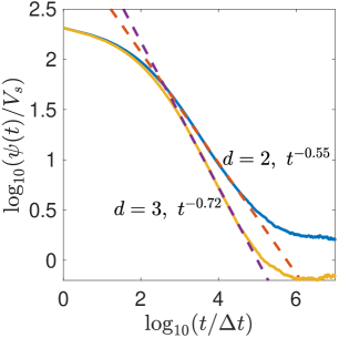
Figure 8: Decay of mean membrane-potential near criticality in $d=2$ and $3$-dimensional lattices for excitatory absorbing state networks with $N=1000$. All neuron membrane potentials start at $V_{i}(0)/V_{s}=0.2$, where $V_{s}$ is a scale factor with units of the membrane potential. Network dynamics are simulated for $1500$ time-steps of size $\Delta t=0.1$ and averaged over $100$ trials. Plots show the population average of these trial averages to eliminate stochastic variability. There is a region of the decay of both curves that is consistent with a power-law $t^{-\beta}$ with exponents that agree with the predicted value $\beta=d/4$.

With this exponent we may use our estimates of $\nu_{\ast}$ and $z_{\ast}$ to calculate the exponents measured in neural avalanches in slice tissue. In slices neurons are not very spontaneously active, and the absorbing state network may be an appropriate model for this situation. A neural avalanche is triggered when a single neuron fires due to external stimulation (either injected by the experimenter or due to environmental noise), and triggers a cascade of subsequent firing events. Key statistical measurements are the distribution of avalanche sizes, $S$, which is predicted to scale as $S^{-\tau_{\ast}}$ for large $S$, the distribution of durations $T$, which is predicted to scale as $T^{-\alpha_{\ast}}$, and the average avalanche size conditioned on the duration, which is predicted to scale as $T^{1/(\sigma_{\ast}\nu_{\ast}z_{\ast})}$ FriedmanPRL2012 . These relations introduce the new critical exponents $\tau_{\ast}$, $\alpha_{\ast}$, and $\sigma_{\ast}$, in addition to the exponents $z_{\ast}=2$, $\beta_{\rm AS}=d/4$, and $\nu_{\ast}$. These critical exponents are not independent, and are related through the scaling relations buice2007field

$$\tau_{\ast} =1+\frac{\beta_{\rm AS}}{(d+z_{\ast})\nu_{\ast}-\beta_{\rm AS}},$$ (34)

$$\sigma_{\ast} =\frac{1}{(d+z_{\ast})\nu_{\ast}-\beta_{\rm AS}},$$ (35)

$$\frac{\alpha_{\ast}-1}{\tau_{\ast}-1} =\frac{1}{\sigma_{\ast}\nu_{\ast}z_{\ast}}.$$ (36)

We use these relations to calculate the critical exponents for networks with effective dimensions $2.78\lesssim d\leq 4$, shown in Fig. 9. These estimates do not agree well with the experimental estimates obtained by FriedmanPRL2012 : a value of $d\approx 3.2\sim 3.4$ yields predictions consistent with the ends of the ranges of the reported error bars ($\tau_{\ast}=1.6\pm 0.2$, $\alpha_{\ast}=1.7\pm 0.2$), but the estimate of $1/(\sigma_{\ast}\nu_{\ast}z_{\ast})=1.3\pm 0.05$ is not consistent with any dimension in this range.

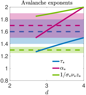
Figure 9: Estimate of the avalanche exponents $\tau_{\ast}$, $\alpha_{\ast}$, and $1/\sigma_{\ast}\nu_{\ast}z_{\ast}$ as a function of the effective dimension $d$ (solid lines), compared to the experimental estimates of these quantities obtained in Ref. FriedmanPRL2012 (dashed lines, with uncertainties shown as shaded regions).

Previous work has suggested that the universality class of neural avalanches may be Directed Percolation, on the basis of experimental measurements that appeared to be consistent with the mean-field estimates buice2007field . Our analysis, based on the high resolution recordings of FriedmanPRL2012 , suggests that a different universality class may describe neural avalanches. This could be due to several factors, including the aforementioned fact that we expect randomness of synaptic connections to alter or obscure the critical exponents. Other important factors include the fact that actual slice networks are unlikely to have symmetric synaptic connections ($J_{ij}\neq J_{ji}$), which could give relevant perturbations to the fixed points, or the effective dimension could lie closer to $d=2$, for which a different critical point may control the universal properties of the absorbing state network.

In the spontaneous network at the spinodal critical point our estimates of $\beta_{\rm spont}$ are straightforwardly calculated from the anomalous exponent $\delta\eta^{X}_{\ast}$: $\beta_{\rm spont}=(d-2)/4-\delta\eta^{X}_{\ast}$. We plot the results in Fig. 10.

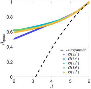
Figure 10: Estimate of the exponent $\beta_{\rm spont}$ for the spinodal fixed point of the spontaneous network model, as a function of the effective dimension $d$, compared to the perturbative expansion in powers of $\sqrt{\epsilon}=\sqrt{6-d}$.

In principle, spontaneous networks can generate avalanche-like activity, realized as large fluctuations from baseline firing. However, we cannot use Eqs. (34)-(36) to estimate avalanche exponents near this fixed point, as spontaneous activity allows for multiple system-spanning avalanches to overlap in time, as seen, e.g., in the random-field Ising model. This introduces a new hyperscaling exponent into the exponent equalities. This hyperscaling exponent can also alter the Harris criterion used to estimate whether disorder is a relevant perturbation to a critical point. Because our estimates of the critical exponents near the spinodal fixed point may not be reliable in dimensions $d\lesssim 5$, and it is unclear whether exponent relations derived for systems with hyperscaling violations would apply to a spinodal fixed point, we do not attempt to estimate the avalanche exponents for spontaneous networks at this juncture.

IV Discussion

In this work we have adapted the “non-perturbative renormalization group” (NPRG) formalism to apply to a spiking network model of neural activity, and used this formalism to study universal and non-universal properties of the network statistics in both lattices and random networks. We have shown that this method

1. produces accurate quantitative predictions of the effective firing rate nonlinearity that describes the relationship between the mean firing rate of neurons and their mean membrane potentials, including excitatory lattices, excitatory graphs of random connections, and random networks with Gaussian synaptic connections (Fig. 3). See Appendix A for additional examples and different choices of the bare nonlinearity $\phi(V)$.

2. qualitatively captures non-universal behavior in the supercritical regime.

3. predicts that the spiking network model supports two important universality classes, a Directed-Percolation universality class in networks with an absorbing state and a spinodal fixed point like the Yang-Lee $\phi^{3}$ theory universality class in spontaneous networks.

4. allows us to estimate values of critical exponents as a function of the effective network dimension $d$.

The non-universal predictions agree well with simulations, demonstrating the success of the extension to network models. We focused on calculating the effective nonlinearity $\Phi_{1}(y)$ using a hierarchy-closing scheme. In the sub-critical regime we are able to close the hierarchy at fourth order, while in the super-critical regime we could only calculate solutions at first order due to the non-analytic behavior that emerges. For similar reasons of numerically instability, we studied the non-universal nonlinearities only in the context of spontaneous networks, not the absorbing state networks that we consider in addition to spontaneous networks when investigating universal quantities. The numerical solution of the flow equations appears unreliable in the region where the bare nonlinearity vanishes, possibly due to the systematic issues observed in the spontaneous case in which the predicted nonlinearity underestimates the simulation data.

Our analysis of universal features makes several qualitative predictions regarding universality classes that spiking neural networks could be part of, though quantitative predictions of critical exponents require further refinement of the method and handling of the randomness of synaptic connections, to be discussed below. To arrive at our results we used a combination of a perturbative and non-perturbative truncations. Both yield roughly consistent results for dimensions not far from the upper critical dimensions $d_{c}$, while higher order non-perturbative truncations give better results in lower dimensions and can predict the existence of fixed points that may not be perturbatively accessible, though the results may still be unreliable far from $d_{c}$ because the local potential approximation neglects the frequency and $\lambda$ dependence of the renormalized terms.

There are several other aspects of our results and their implications for neuroscience research that warrant detailed discussion, including the anomalous dimensions (IV.1), limitations of the spiking model we use here and the local potential approximation (IV.2), the role of disorder in the synaptic weight matrix $J_{ij}$ (IV.3), and potential implications for the critical brain hypothesis (IV.4), to be discussed in turn below.

IV.1 Anomalous dimensions

In the standard NPRG approach in statistical physics on lattices or continuous media, anomalous exponents—$\delta\eta^{X}_{\ast}$ in this work—are best characterized by including the long-time, small momentum behavior of the model, which is not captured by the local potential approximation. Improved quantitative estimates can often be obtained by including field renormalization factors in the ansatz for the average effective action, dubbed the LPA’ approximation. In the spontaneous network model our non-trivial choices of the running scale $\tilde{X}_{\Lambda}$ are effectively like including a field renormalization of the noise, though is perhaps more like the redundant parameter in directed percolation field theories Janssen2004pair , as our Ward-Takahashi identities do not allow for direct field renormalization factors.

In order to improve on the predictions of the LPA’ approach, previous NPRG work has implemented the “derivative expansion,” which amounts to expanding renormalized parameters as functions of the momentum and temporal frequency. In the spiking network model such an extension might involve expanding the function $U_{\Lambda}(\tilde{x},y)$ in powers of the frequency $\omega$ and synaptic weight matrix eigenvalues $\lambda$. The derivative expansion has yielded very accurate estimates of critical exponents in the $O(N)$ model universality classes canet2003nonperturbative , though the technical implementation has been found to be sensitive to the smoothness of the regulator morris1994derivative ; morris1998properties . Our eigenvalue regulator (13) is equivalent to the ultra-sharp regulator that has been used in previous NPRG approaches, which is known to cause issues for the derivative expansion.

An alternate approach to obtaining improved estimates of the anomalous exponents is a type of hierarchy closure scheme for vertex functions (derivatives of $\Gamma$), not related to our hierarchy Eqs. (15), called the Blaizot–Méndez-Galain–Wschebor (BMW) approximation blaizot2005non . stapmanns2020self introduce a variation of this approximation technique for a firing rate model. This could potentially be an approach that works even with our ultra-sharp regulator.

While the beyond-LPA methods discussed above may improve our estimates of the critical exponents, they are unlikely to yield a non-trivial value of the dynamic exponent $z_{\ast}=2$ imposed by our Ward-Takahashi identities. This poses a mystery, as the critical points we have identified for this model appear to be closely related to the directed percolation universality class in absorbing state networks and the Ising model family with explicitly broken $\mathbb{Z}_{2}$ symmetry in spontaneous networks, but the fact that $z_{\ast}=2$ would suggest these fixed points belong to distinct universality classes.

There is some precedent for this situation: there are non-equilibrium extensions of the Ising model that share static critical exponents of the equilibrium Ising universality class, but have different dynamic critical exponents, the best-known examples being the so-called “Model A” and “Model B” formulations tauber2007field ; tauber2012renormalization ; tauber2014critical .

We conjecture that the trivial dynamical exponent is due to the linear dynamics of the membrane potential in Eq. (1), which was an important element of the derivation of one of our Ward-Takahashi identities. Including additional nonlinearities in the membrane dynamics—which would couple $V_{i}(t)$ nonlinearly to its response field $\tilde{V}_{i}(t)$ and not just the spike response field $\tilde{n}_{i}(t)$ in the action (5)—would give rise to non-trivial values of $z_{\ast}$. We discuss this possibility in more detail in the next section.

IV.2 Limitations of the spiking model and the local potential approximation

The spiking network we have focused on here is a prototypical model in neuroscience and captures many of the essential features of spiking network activity. However, there are possible changes to the model that could alter the critical properties we estimate in this work. The main features we discuss here are the form of the dynamics of the membrane potentials and spike train generation, as well as the properties of the synaptic connections.

As noted in the previous section, the dynamic response of the membrane potentials to spike input is linear in Eq. (1). Although spike generation depends nonlinearly on the membrane potential through the conditional Poisson process, Eq. (2), the linearity of the membrane potential dynamics allows us to solve for $V_{i}(t)$ entirely in terms of the spike trains $\dot{n}_{i}(t)$. It is this feature that allows us to derive one of the Ward-Takahashi identities that restricts the form of the average effective action $\Gamma[\tilde{\psi},\psi,\tilde{\nu},\nu]$. If the membrane potential dynamics contain a nonlinear dependence $F(V)$, for example,

$$\tau\frac{dV_{i}(t)}{dt}=-(V_{i}(t)-\mathcal{E}_{i})+F(V_{i}(t))+\sum_{j=1}^{N}J_{ij}\dot{n}_{j}(t),$$

then the solution for $V_{i}(t)$ will depend nonlinearly on the spike trains, which precludes the derivation of one of the Ward-Takahashi identity that relied on integrating out the membrane potential fields. The other Ward-Takahashi identity, which involved integrating out the spiking fields, remains. Consequently we can only restrict the form of the average effective action to

$$\Gamma[\chi]=\tilde{\nu}\cdot\nu-\tilde{\psi}\cdot J\cdot\nu+\Upsilon[\tilde{\psi},\psi,\tilde{\nu}].$$

i.e., the renormalized terms would be functionals of three fields, instead of just $\tilde{\nu}$ and $\psi$. In this situation, the fact that the average effective action has the same structure as the bare action, plus all terms allowed by symmetry, becomes crucial, and the standard course of action is to make an ansatz that to lowest order $\Gamma$ has the same form as the bare action but with renormalized coefficients, e.g.,

$$\Gamma_{\Lambda}[\chi] =\int\sum_{i}\Bigg{\{}\tilde{\psi}_{i}(t)\Bigg{[}\tau_{\Lambda}\dot{\psi}_{i}(t)+\psi_{i}(t)-\mathcal{E}_{i}-F_{\Lambda}(\psi_{i}(t))$$

$$\hskip 85.35826pt-\sum_{j}J_{ij}(t-t^{\prime})\nu_{j}(t^{\prime})\Bigg{]}$$

$$\hskip 79.6678pt+\tilde{\nu}_{i}(t)\nu_{i}(t)-U_{\Lambda}(\tilde{\nu}_{i}(t),\psi_{i}(t))\Bigg{\}},$$

where the membrane time constant $\tau_{\Lambda}$ and nonlinearity $F_{\Lambda}(\psi)$ flow in addition to $U_{\Lambda}(\tilde{x},y)$. Because these parameters flow they can contribute to the anomalous exponents in a way that was absent in the linear model. In particular, if $\tau_{\Lambda}\sim\delta\Lambda^{-\delta z_{\ast}/2}$ as $\delta\Lambda\rightarrow 0$, then the dynamic exponent would become $z_{\ast}=2+\delta z_{\ast}$; i.e., the dynamic exponent may no longer take on the trivial value $z_{\ast}=2$. Moreover, the membrane potential nonlinearity could also allow for the possibility of partly canceling out terms arising from the firing rate nonlinearity $\Phi_{\Lambda}(\psi)$, which we expect would allow the network model to admit the fixed point found recently in a firing rate network model via a perturbative approach tiberi2022gell .

Another important type of membrane nonlinearity is a multiplicative coupling between the membrane potential and the spike train. In this stochastic spiking model a coupling of the form $\tilde{V}_{i}(t)\dot{n}_{i}(t)\left(V_{i}(t)-\mathcal{E}_{\rm reset}\right)$ has been used to implement a hard reset of the membrane potential to $\mathcal{E}_{\rm reset}$ after a neuron spikes ocker2022dynamics , as opposed to the soft resets implemented through negative diagonal terms $J_{ii}<0$. Similarly, the synaptic currents that neurons inject into their targets depends on the membrane potential of the target, known as conductance-based coupling gerstner2014neuronal , which would replace the synaptic current injection $\tilde{V}_{i}(t)J_{ij}\dot{n}_{j}(t)$ in Eq. (1) with $-\tilde{V}_{i}(t)\left(V_{i}(t)-\mathcal{E}_{\rm syn}\right)G_{ij}\dot{n}_{j}(t)$, for some synaptic reversal potential $\mathcal{E}_{\rm syn}$ and conductances $G_{ij}$. Many types of behavior observed in conductance-based models can be reproduced with current based models, so this type of interaction could be irrelevant in the RG sense, at least near some critical points, but checking this could be challenging. These types of interactions would require a modified approach using the NPRG method presented here, as they not only introduce a direct coupling between the spike train fields $\dot{n}_{i}(t)$ and the membrane potentials $V_{i}(t)$ in the model, but in the conductance-based model the synaptic interactions are no longer bilinear, and cannot be used to regulate the flow of models from the mean-field theory to the true model. A separate regulator would have to be introduced, perhaps more in the style of standard NPRG work that achieves mean-field theory as a starting point by introducing a large “mass” term to freeze out stochastic fluctuations. We discuss a possible form of such a regulator in SuppInfo .

Finally, a notable simplification of the analysis presented here is the restriction to symmetric synaptic connections $J_{ij}=J_{ji}$. While in principle our method will work for asymmetric matrices, the assumption of symmetry allows a dramatic simplification of the general flow equation for the local potential $U_{\Lambda}(\tilde{x},y)$ (Eq. (11)), after which the $N\rightarrow\infty$ limit could be taken. While symmetric connections have been very useful in developing foundational theories in neuroscience, such as associative memory models like the Hopfield network hopfield1982neural , real neural circuits do not have perfectly symmetric connections. Connections are often highly reciprocally connected song2005highly , and hence symmetric weights may be a reasonable approximation for some circuits; however, the behavior of firing rate networks is known to change qualitatively as the correlations between $J_{ij}$ and $J_{ji}$ vary from $1$ to $0$. For example, firing rate networks with perfectly symmetric connections exhibit spin-glass behavior with many metastable states sompolinsky1982relaxational , while non-symmetric connections display a transition to chaotic behavior SompolinskyPRL1988 ; kadmon2015transition . In-between new phases controlled by marginally stable stables have even been shown to emerge berlemont2022glassy . We therefore expect correlations of reciprocal connections to be a relevant parameter in the RG flow of the spiking network model.

Allowing for asymmetric connections would also allow exploration of networks with multiple cell types, the classic case in neuroscience being populations of separate excitatory and inhibitory neurons (“E-I networks”), whose synapses are constrained to be positive or negative, respectively. These different population could have different effective firing rate nonlinearities, owing to their different properties, which would not be captured by the current formalism. This said, models in which the E-I dichotomy is not enforced can be viewed as effective models describing networks with unobserved neurons influencing the activity of recorded neurons brinkman2018predicting . In this case our random network model might still capture some aspects of E-I networks, though it may miss some collective phases driven by having cell types bressloff2010metastable .

IV.3 Impact of disorder on critical properties

Much of the renormalization group analysis presented was not affected by the whether neurons were connected in a stuctured arrangement like a lattice or in a random network. Our calculation of the effective nonlinearity $\Phi_{1}(y)$ was insensitive to the origin of the eigenvalue density. Similarly, we find that the critical fixed points of the dimensionless flow equations only depend on the effective dimension $d$ of the network, defined by the scaling of the eigenvalue distribution near the maximum bulk eigenvalue, $\rho_{\lambda}(\lambda)\sim|\Lambda_{\rm max}-\lambda|^{d/2-1}$. Consequently, at the level of the local potential approximation we make in this work, lattices of spatial dimension $d$ and random networks of effective dimension $d$ share the same critical points, and may belong to the same universality class.

However, this conclusion is likely too naive. For one, extensions of the NPRG beyond the local potential approximation (e.g., by generalizing the derivative expansion or implementing a BMW-esque closure scheme) may not have the convenient property that the eigenmodes of the weight distribution fall out of the flow equations, and hence could shape the critical properties of the network. This could even happen at the level of the LPA in asymmetric networks.

Second, we have already shown that the macroscopic dimensionful behavior of the system does depend on details of the synaptic weights $J_{ij}$. For instance, excitatory networks show two extremal metastable states (Fig. 1A), while random networks with excitatory and inhibitory connections are expected to exhibit spin-glass behavior.

It is well known that “disorder,” such as a random distribution of synaptic connections, can alter the critical properties of a continuous phase transition GoldenfeldBook1992 . In equilibrium the Harris criterion predicts that when the correlation length exponent $\nu_{\ast}<2/d$, then disorder is a relevant perturbation to a critical point. Similar criteria also appear to hold in non-equilibrium absorbing state transitions hooyberghs2004absorbing . If we assume this criterion holds for the spiking network model, then for the absorbing state $\nu_{\ast}-2/d<0$ for the estimates shown in Fig. 5, and we expect disorder to be relevant. In the spontaneous network model it is not clear if a Harris-like criterion applies to the spinodal point, which is associated with a first order transition.

One way to investigate how disorder impacts the behavior of the network would be to perform a dynamic mean-field calculation similar to those used to study the population statistics of mean-field models (we give the set up of such a calculation in the Supplementary Material SuppInfo ). The primary challenge of this approach is the non-analytic behavior of the effective nonlinearity at and above the critical point, as the self-consistent calculations necessarily involve expectations over the nonlinearity.

An alternate route to investigating the impact of disorder on critical points in the dimensionless RG flow is by means of a replica calculation, and tracking the RG flow of an additional function called the “disorder cumulant,” which has been done for the random-field $O(N)$ model tarjus2004nonperturbative ; tarjus2008nonperturbative1 ; tissier2008nonperturbative2 ; balog2015activated . Understanding the impact of disorder on critical properties of spiking networks, and the influence on the sub- or super-critical collective behavior, while important, is non-trivial, and we leave investigations of these matters as avenues for future work.

IV.4 Implications for the critical brain hypothesis

Many experimental searches for criticality in neural tissue have focused on neural avalanches beggs2003neuronal ; BeggsFrontPhysio2012 ; buice2007field ; FriedmanPRL2012 , which display power law scaling in the distributions of quantities like avalanche size, duration, and even scaling forms of avalanche shapes FriedmanPRL2012 . Other lines of inquiry have looked for general signatures of criticality in, e.g., the retina tkavcik2015thermodynamics . These experimental analyses have spawned a variety of theoretical models to explain power law observations in neural data, including analyses that claim that many signatures of criticality may appear in non-critical models touboul2010can ; touboul2017power , or could be due to the effects of subsampling nonnenmacher2017signatures ; levina2017subsampling .

To date, most experimental analyses of criticality have looked for power law scaling, with a smaller subset attempting to perform Widom-style data collapses, a stronger signature of criticality FriedmanPRL2012 . Theoretically, most work has either focused on simulating network models that can produce power-law scaling in neural activity statistics, performed mean-field analyses to identify phases williams2014quasicritical , or reinterpreted known models in statistical physics whose phase transition properties are well-studied buice2007field . The first and second cases typically do not directly invoke the renormalization group, and in the latter case the renormalization group may have been used to analyze models in their original context, but the reinterpretation in neuroscience must often be taken as a coarse-grained model of neural activity, rather than spiking activity.

Recent applications of renormalization group methods in neuroscience include bradde2017pca ; meshulam2019coarse which used ideas of renormalization-style coarse-graining as a data analysis tool. tiberi2022gell applied perturbative RG to the Wilson-Cowan neural field model, a model of coarse-grained neural activity, and found that in $d=2$ the model exhibits marginal scaling, leading to scale-dependent logarithmic corrections to critical exponents. There has been some work applying the non-perturbative renormalization group in a neuroscience context, notably stapmanns2020self introduces a BMW-like scheme for calculating correlation functions in firing rate models, and kline2022gaussian explores possible equivalences between the NPRG and the information bottleneck neck in information theory, used in neural sensory coding work. To the author’s knowledge, the present work is the first to apply renormalization group methods to spiking network models, both to calculate non-universal quantities like the firing rate nonlinearity, and to investigate critical points in the renormalization group flow.

Our results demonstrate that a spiking network model commonly used in neuroscience does possess non-trivial critical points in its renormalization group flow, and moreover that these critical points are accessed by tuning the gain of the neurons $\phi^{\prime}(0)$ or the strength of the synaptic connections $\Lambda_{\rm max}$ —in contrast to the possibility that such critical points may not be accessible and mean-field theory describes transitions in neural activity, or more exotic possibilities like non-universal scaling. In networks with absorbing states our analysis predicts a regular continuous phase transition between an inactive state and an active state, which could be the universality class of avalanche dynamics observed in vitro, where the spontaneous activity of neurons is very low. In spontaneously active networks, however, which might be a better model for in vivo activity, our analysis predicts that the fixed point corresponds to a discontinuous transition associated with a spinodal point, owing to the fact that the dimensionless couplings are complex-valued. Despite the fact that this fixed point corresponds to a first order transition, it still boasts universal scaling. Thus, our results establish a firm renormalization-group-based foundation for the possibility that real networks could potentially be tuned to such critical points, but the full picture of the nature of these transitions may be more complicated than the relatively simple second order transitions commonly associated with universality.

This said, it is important to distinguish between the possibility that neural circuit dynamics posses bona fide critical points separating different regimes of emergent collective activity from some of the stronger variations of the critical brain hypothesis, which posit that the brain’s homeostatic mechanisms actively maintain neural activity near a critical point. The results presented here say nothing about whether the brain tends to maintain itself near critical points. The most-studied mechanism by which the brain might tune itself to a critical point is through synaptic plasticity, a process through which the activity of the network alters the synaptic connections $J_{ij}$. The model presented here assumes fixed $J_{ij}$, but in principle one could add such dynamics to $J_{ij}$ and study how this changes the renormalization group flow. This scenario is conceptually similar to direction percolation with a conserved quantity (DP-C) discussed earlier in this report, in which giving dynamics to a previously conserved quantity changes the critical exponents janssen2005field .

V Future directions

We have shown that we can extend the methods of the non-perturbative renormalization group (NPRG) to apply to an action for which the free theory is a Poisson, rather than Gaussian, process. Moreover, the dynamics may take place on either networks or lattices. While the context of our investigation is the collective activity of neural populations, the underlying model has been applied to spike-like events in other fields, including epidemiology, ecology, and earth science SkrondalNorskEpi2003 ; WartonAnnAppStats2010 ; BrayStatSci2013 ; brinkman2015probing ; brinkman2016probabilistic .

While the spiking network model presented here contains many simplifications that do not reflect the physiology of real neural circuitry, this has allowed it to become an important foundational model for extending the non-perturbative renormalization group to spiking neural networks with increasingly realistic features. In our discussion we have outlined many possible avenues for future extensions of the model and methods, including going beyond the local potential approximation, adding nonlinearities to the membrane potential dynamics, investigating how randomness in synaptic connections might alter critical properties, and investigating other network structures—in particular asymmetric networks and networks with multiple cell types.

Other avenues that can be investigated with the current model include studying the effects of fluctuations on dynamic phenemona, such as spinodal decomposition. Our finding that the spontaneous networks are controlled by a spinodal fixed point motivated investigating how a sudden quench—a change of the bare gain $\phi^{\prime}(0)$—could lead to phase separation, as shown in Fig. 1. A mean-field analysis of the dynamics would predict that one phase of the network typically takes over rather quickly, while simulations show that the stochastic fluctuations give rise to more complex spatiotemporal dynamics. Our method provides a means of taking the stochastic fluctuations into account in both the sub- and super-critical phases. Moreover, because our method is not restricted to lattices, we can probe deeper into the impact that other network structures have; a particular case of interest will be navigable-small world graphs, which interpolate from the lattice dynamics shown in Fig. 1A to the random network dynamics shown in Fig. 1B. By adapting the non-perturbative renormalization group to spiking networks, we have opened new doors to elucidating such phenomena.

Appendix A Examples of effective nonlinearities for different networks and nonlinearities

Here we provide some additional examples of our NPRG method applied to different types of networks with different effective dimensions $d$ (Figs. 12-14) and nonlinearities $\phi(y)$ (Fig. 11). (c.f., Fig. 3, shown for $d=3$ and a sigmoidal nonlinearity).

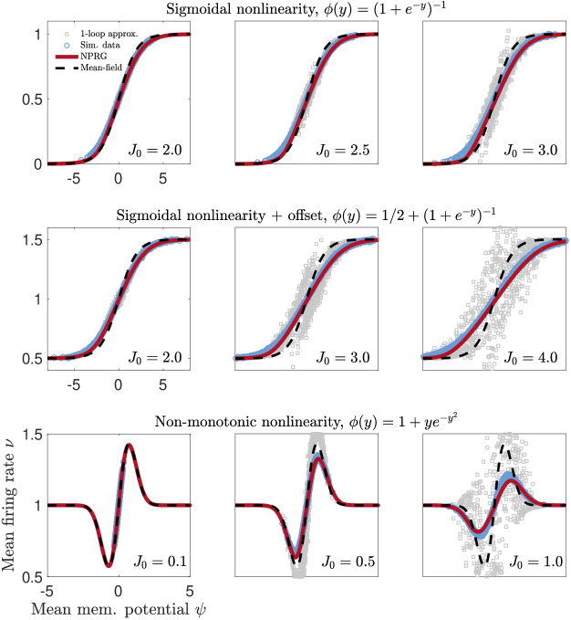
Figure 11: Effective nonlinearities as functions of synaptic strength in networks of $N=10^{3}$ neurons and for three different choices of the bare nonlinearity $\phi(V)$ (in dimensionless units). Top row: Sigmoidal nonlinearity $\phi(y)=(1+\exp(-y))^{-1}$ and synaptic weight variance $J_{0}=2.0$ (left) $2.5$ (middle), and $3.0$ (right). Middle row: Sigmoidal nonlinearity with a non-zero minimum baseline firing rate, $\phi(y)=1/2+1/(1+\exp(-y))$ and synaptic weight variance $J_{0}=2.0$ (left) $3.0$ (middle), and $4.0$ (right). Bottom: Results for a non-monotonic nonlinearity with $\phi(y)=1+y\exp(-y^{2})$ and synaptic weight variance $J_{0}=0.1$ (left) $0.5$ (middle), and $1.0$ (right). Our non-perturbative renormalization group analysis predicts that scatter-plots of the mean firing rates $\nu_{i}$ versus mean membrane potentials $\psi_{i}=\mathcal{E}_{i}+\sum_{i}J_{ij}\nu_{j}$ should lie along a nonlinear curve, confirmed by the simulation data (blue data points). Our prediction of the effective nonlinearity is given by the solid red curve, obtained by solving Eq. (14) numerically. For comparison, we show the mean field prediction (black dashed lines) and the $1$-loop predictions obtained using Ref. OckerPloscb2017 ’s diagrammatic methods (grey data points). We see that for strong coupling strengths our non-perturbative predictions continue to predict the firing rates well when other methods break down.

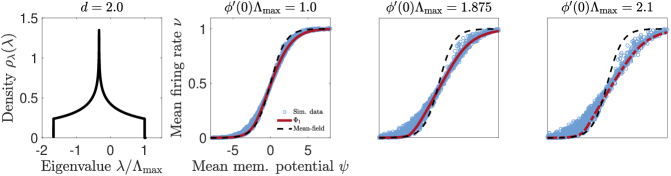
Figure 12: Effective nonlinearities on a hypercubic lattices of dimensions $d=2$, along with the corresponding eigenvalue distributions $\rho_{\lambda}(\lambda)$ (far left). We show a subcritical nonlinearity (left), a near-critical nonlinearity (middle), and a supercritical nonlinearity (right). The red curves are the predictions of the hierarchy of nonlinearities (Eqs. (15), truncated at fourth order for subcritical and critical cases and first order for the supercritical case, using the results of loh2011accurate to compute the eigenvalue distributions. Blue data points are simulated data, using a network of $N=35^{2}$ neurons.

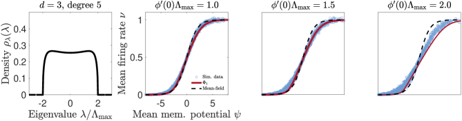
Figure 13: Effective nonlinearities on excitatory random regular graphs of effective dimension $d=3$ (all cases) and degrees $5$ (top row) and $3$ (bottom row), along with their corresponding eigenvalue distributions $\rho_{\lambda}(\lambda)$ (far left). For each degree we show a subcritical nonlinearity (left), a near-critical nonlinearity (middle), and a supercritical nonlinearity (right), tuned by varying the global excitatory coupling $J_{0}=\Lambda_{\rm max}/2$. We map out the nonlinearity synthetically by assigning a distribution of rest potentials $\mathcal{E}_{i}$. The red curves are the predictions of the hierarchy of nonlinearities (Eqs. (15), truncated at fourth order for subcritical and near-critical cases and first order for the supercritical case. Blue data points are simulated data, using networks of $N=10^{3}$ neurons.

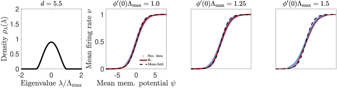
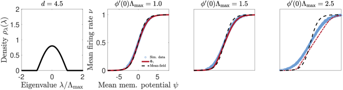
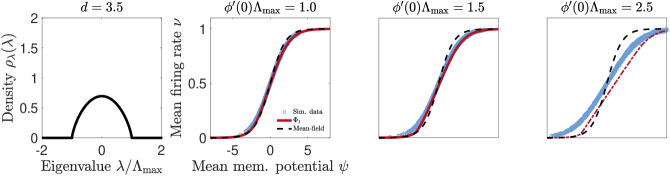
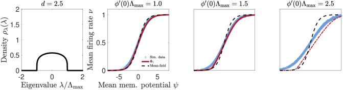
Figure 14: Effective nonlinearities on random networks of effective dimensions $d=5.5$ (top row) to $d=2.5$ (bottom row), along with their corresponding eigenvalue distributions $\rho_{\lambda}(\lambda)$ (far left). For each dimension we show a subcritical nonlinearity (left), a near-critical nonlinearity (middle), and a supercritical nonlinearity (right), although the networks themselves are not critical due to the heterogeneity of the neurons. The red curves are the predictions of the hierarchy of nonlinearities (Eqs. (15), truncated at fourth order for subcritical and critical cases and first order for the supercritical case, using the results of loh2011accurate to compute the eigenvalue distributions. Blue data points are simulated data, using networks of $N=10^{3}$ neurons. Networks are created by generating a symmetric Gaussian random matrix, diagonalizing it, and drawing new eigenvalues from a Beta distribution SuppInfo .

References

- [1] R. E. Kass, S.-I. Amari, K. Arai, E. N. Brown, C. O. Diekman, M. Diesmann, B. Doiron, U. T. Eden, A. L. Fairhall, G. M. Fiddyment, T. Fukai, So. Grün, M. T. Harrison, M. Helias, H. Nakahara, J.-N. Teramae, P. J. Thomas, M. Reimers, J. Rodu, H. G. Rotstein, E. Shea-Brown, H. Shimazaki, S. Shinomoto, B. M. Yu, and M. A. Kramer. Computational neuroscience: Mathematical and statistical perspectives. Annual Review of Statistics and Its Application, 5(1):183–214, 2018.
- [2] A. A. Faisal, L.P. J. Selen, and D. M. Wolpert. Noise in the nervous system. Nat. Rev. Neurosci., 9(4):292–303, 2008.
- [3] Mikhail I Rabinovich, Pablo Varona, Allen I Selverston, and Henry DI Abarbanel. Dynamical principles in neuroscience. Reviews of modern physics, 78(4):1213, 2006.
- [4] Kechen Zhang. Representation of spatial orientation by the intrinsic dynamics of the head-direction cell ensemble: a theory. Journal of Neuroscience, 16(6):2112–2126, 1996.
- [5] Carlo R Laing and Carson C Chow. Stationary bumps in networks of spiking neurons. Neural computation, 13(7):1473–1494, 2001.
- [6] Klaus Wimmer, Duane Q Nykamp, Christos Constantinidis, and Albert Compte. Bump attractor dynamics in prefrontal cortex explains behavioral precision in spatial working memory. Nature neuroscience, 17(3):431–439, 2014.
- [7] Sung Soo Kim, Hervé Rouault, Shaul Druckmann, and Vivek Jayaraman. Ring attractor dynamics in the drosophila central brain. Science, 356(6340):849–853, 2017.
- [8] G Bard Ermentrout and Jack D Cowan. A mathematical theory of visual hallucination patterns. Biological cybernetics, 34(3):137–150, 1979.
- [9] Paul C Bressloff. Metastable states and quasicycles in a stochastic wilson-cowan model of neuronal population dynamics. Physical Review E, 82(5):051903, 2010.
- [10] Thomas Charles Butler, Marc Benayoun, Edward Wallace, Wim van Drongelen, Nigel Goldenfeld, and Jack Cowan. Evolutionary constraints on visual cortex architecture from the dynamics of hallucinations. Proceedings of the National Academy of Sciences, 109(2):606–609, 2012.
- [11] H. Sompolinsky, A. Crisanti, and H. J. Sommers. Chaos in random neural networks. Phys. Rev. Lett., 61:259–262, Jul 1988.
- [12] David Dahmen, Sonja Grün, Markus Diesmann, and Moritz Helias. Second type of criticality in the brain uncovers rich multiple-neuron dynamics. Proceedings of the National Academy of Sciences, 116(26):13051–13060, 2019.
- [13] John M Beggs and Dietmar Plenz. Neuronal avalanches in neocortical circuits. Journal of neuroscience, 23(35):11167–11177, 2003.
- [14] Michael A Buice and Jack D Cowan. Field-theoretic approach to fluctuation effects in neural networks. Physical Review E, 75(5):051919, 2007.
- [15] N. Friedman, S. Ito, B. A. W. Brinkman, M. Shimono, R. E. L. DeVille, K. A. Dahmen, J. M. Beggs, and T. C. Butler. Universal critical dynamics in high resolution neuronal avalanche data. Phys. Rev. Lett., 108:208102, May 2012.
- [16] Jonathan Kadmon and Haim Sompolinsky. Transition to chaos in random neuronal networks. Physical Review X, 5(4):041030, 2015.
- [17] Woodrow L Shew, Hongdian Yang, Shan Yu, Rajarshi Roy, and Dietmar Plenz. Information capacity and transmission are maximized in balanced cortical networks with neuronal avalanches. Journal of neuroscience, 31(1):55–63, 2011.
- [18] J. Beggs and N. Timme. Being critical of criticality in the brain. Frontiers in Physiology, 3:163, 2012.
- [19] W. L. Shew and D. Plenz. The functional benefits of criticality in the cortex. The Neuroscientist, 19(1):88–100, 2013. PMID: 22627091.
- [20] Jonathan Touboul and Alain Destexhe. Can power-law scaling and neuronal avalanches arise from stochastic dynamics? PloS one, 5(2):e8982, 2010.
- [21] Jonathan Touboul and Alain Destexhe. Power-law statistics and universal scaling in the absence of criticality. Physical Review E, 95(1):012413, 2017.
- [22] Marcel Nonnenmacher, Christian Behrens, Philipp Berens, Matthias Bethge, and Jakob H Macke. Signatures of criticality arise from random subsampling in simple population models. PLoS computational biology, 13(10):e1005718, 2017.
- [23] Anna Levina and Viola Priesemann. Subsampling scaling. Nature communications, 8(1):1–9, 2017.
- [24] G. K. Ocker, K. Josić, E. Shea-Brown, and M. A. Buice. Linking structure and activity in nonlinear spiking networks. PLOS Computational Biology, 13(6):1–47, 06 2017.
- [25] Jonas Stapmanns, Tobias Kühn, David Dahmen, Thomas Luu, Carsten Honerkamp, and Moritz Helias. Self-consistent formulations for stochastic nonlinear neuronal dynamics. Physical Review E, 101(4):042124, 2020.
- [26] M. Kordovan and S. Rotter. Spike train cumulants for linear-nonlinear poisson cascade models, 2020.
- [27] Gabriel Koch Ocker. Dynamics of stochastic integrate-and-fire networks. Phys. Rev. X, 12:041007, Oct 2022.
- [28] L. Canet, B. Delamotte, O. Deloubrière, and N. Wschebor. Nonperturbative renormalization-group study of reaction-diffusion processes. Phys. Rev. Lett., 92:195703, May 2004.
- [29] Léonie Canet, Hugues Chaté, Bertrand Delamotte, Ivan Dornic, and Miguel A Munoz. Nonperturbative fixed point in a nonequilibrium phase transition. Physical review letters, 95(10):100601, 2005.
- [30] T. Machado and N. Dupuis. From local to critical fluctuations in lattice models: A nonperturbative renormalization-group approach. Phys. Rev. E, 82:041128, Oct 2010.
- [31] L. Canet, H. Chaté, and B. Delamotte. General framework of the non-perturbative renormalization group for non-equilibrium steady states. Journal of Physics A: Mathematical and Theoretical, 44(49):495001, Nov 2011.
- [32] A. Rançon and N. Dupuis. Nonperturbative renormalization group approach to strongly correlated lattice bosons. Phys. Rev. B, 84:174513, Nov 2011.
- [33] A. A. Winkler and E. Frey. Long-range and many-body effects in coagulation processes. Phys. Rev. E, 87:022136, Feb 2013.
- [34] Ingo Homrighausen, Anton A. Winkler, and Erwin Frey. Fluctuation effects in the pair-annihilation process with lévy dynamics. Phys. Rev. E, 88:012111, Jul 2013.
- [35] T. Kloss, L. Canet, B. Delamotte, and N. Wschebor. Kardar-parisi-zhang equation with spatially correlated noise: A unified picture from nonperturbative renormalization group. Phys. Rev. E, 89:022108, Feb 2014.
- [36] Ivan Balog and Gilles Tarjus. Activated dynamic scaling in the random-field ising model: A nonperturbative functional renormalization group approach. Physical Review B, 91(21):214201, 2015.
- [37] Léonie Canet, Bertrand Delamotte, and Nicolás Wschebor. Fully developed isotropic turbulence: Symmetries and exact identities. Physical Review E, 91(5):053004, 2015.
- [38] P. Jakubczyk and A. Eberlein. Thermodynamics of the two-dimensional model from functional renormalization. Phys. Rev. E, 93:062145, Jun 2016.
- [39] C. Duclut and B. Delamotte. Nonuniversality in the erosion of tilted landscapes. Phys. Rev. E, 96:012149, Jul 2017.
- [40] Leenoy Meshulam, Jeffrey L Gauthier, Carlos D Brody, David W Tank, and William Bialek. Coarse graining, fixed points, and scaling in a large population of neurons. Physical review letters, 123(17):178103, 2019.
- [41] Serena Bradde and William Bialek. PCA meets RG. Journal of statistical physics, 167(3):462–475, 2017.
- [42] Lorenzo Tiberi, Jonas Stapmanns, Tobias Kühn, Thomas Luu, David Dahmen, and Moritz Helias. Gell-mann–low criticality in neural networks. Physical Review Letters, 128(16):168301, 2022.
- [43] Daniel Martí, Nicolas Brunel, and Srdjan Ostojic. Correlations between synapses in pairs of neurons slow down dynamics in randomly connected neural networks. Physical Review E, 97(6):062314, 2018.
- [44] Braden AW Brinkman, Fred Rieke, Eric Shea-Brown, and Michael A Buice. Predicting how and when hidden neurons skew measured synaptic interactions. PLoS computational biology, 14(10):e1006490, 2018.
- [45] Bertrand Delamotte. An introduction to the nonperturbative renormalization group. In Renormalization group and effective field theory approaches to many-body systems, pages 49–132. Springer, 2012.
- [46] Léonie Canet. Reaction–diffusion processes and non-perturbative renormalization group. Journal of Physics A: Mathematical and General, 39(25):7901, 2006.
- [47] L. Canet and H. Chaté. A non-perturbative approach to critical dynamics. Journal of Physics A: Mathematical and Theoretical, 40(9):1937–1949, feb 2007.
- [48] Nicolas Dupuis, L Canet, Astrid Eichhorn, W Metzner, Jan M Pawlowski, M Tissier, and N Wschebor. The nonperturbative functional renormalization group and its applications. Physics Reports, 910:1–114, 2021.
- [49] Braden A. W. Brinkman. Supplemental material.
- [50] C. Wetterich. Exact evolution equation for the effective potential. Physics Letters B, 301(1):90 – 94, 1993.
- [51] Jean-Michel Caillol. The non-perturbative renormalization group in the ordered phase. Nuclear Physics B, 855(3):854–884, 2012.
- [52] James Cooper Robinson and C Pierre. Infinite-dimensional dynamical systems: An introduction to dissipative parabolic pdes and the theory of global attractors. cambridge texts in applied mathematics. Appl. Mech. Rev., 56(4):B54–B55, 2003.
- [53] Yen Lee Loh. Accurate calculation of green functions on the d-dimensional hypercubic lattice. Journal of Physics A: Mathematical and Theoretical, 44(27):275201, 2011.
- [54] Juergen Berges, Nikolaos Tetradis, and Christof Wetterich. Non-perturbative renormalization flow in quantum field theory and statistical physics. Physics Reports, 363(4-6):223–386, 2002.
- [55] Nigel Goldenfeld. Lectures on Phase Transitions and the Renormalization Group. Westview Press, 1992.
- [56] Solving Burger’s equation with NDSolve at large time. StackExchange; accessed January 18 2023.
- [57] Haim Sompolinsky and Annette Zippelius. Relaxational dynamics of the edwards-anderson model and the mean-field theory of spin-glasses. Physical Review B, 25(11):6860, 1982.
- [58] Jannis Schuecker, Sven Goedeke, and Moritz Helias. Optimal sequence memory in driven random networks. Physical Review X, 8(4):041029, 2018.
- [59] Aslı Tuncer and Ayşe Erzan. Spectral renormalization group for the gaussian model and 4 theory on nonspatial networks. Physical Review E, 92(2):022106, 2015.
- [60] Hans-Karl Janssen, Frédéric van Wijland, Olivier Deloubrière, and Uwe C. Täuber. Pair contact process with diffusion: Failure of master equation field theory. Phys. Rev. E, 70:056114, Nov 2004.
- [61] Hans-Karl Janssen and Uwe C Täuber. The field theory approach to percolation processes. Annals of Physics, 315(1):147–192, 2005.
- [62] Malo Tarpin, Federico Benitez, Léonie Canet, and Nicolás Wschebor. Nonperturbative renormalization group for the diffusive epidemic process. Physical Review E, 96(2):022137, 2017.
- [63] Malte Henkel, Haye Hinrichsen, and Sven Lübeck. Universality classes different from directed percolation. Non-Equilibrium Phase Transitions: Volume I: Absorbing Phase Transitions, pages 197–259, 2008.
- [64] Fan Zhong. Imaginary fixed points can be physical. Physical Review E, 86(2):022104, 2012.
- [65] Fan Zhong. Renormalization-group theory of first-order phase transition dynamics in field-driven scalar model. Frontiers of Physics, 12(5):1–31, 2017.
- [66] Xin An, David Mesterházy, and Mikhail A Stephanov. Functional renormalization group approach to the yang-lee edge singularity. Journal of High Energy Physics, 2016(7):1–19, 2016.
- [67] Tim R Morris. Properties of derivative expansion approximations to the renormalization group. International Journal of Modern Physics B, 12(12n13):1343–1354, 1998.
- [68] Léonie Canet, Bertrand Delamotte, Dominique Mouhanna, and Julien Vidal. Nonperturbative renormalization group approach to the ising model: a derivative expansion at order . Physical Review B, 68(6):064421, 2003.
- [69] Tim R Morris. Derivative expansion of the exact renormalization group. Physics Letters B, 329(2-3):241–248, 1994.
- [70] J-P Blaizot, R Mendez Galain, and N Wschebor. Non-perturbative renormalization group calculation of the transition temperature of the weakly interacting bose gas. EPL (Europhysics Letters), 72(5):705, 2005.
- [71] Uwe C Täuber. Field-theory approaches to nonequilibrium dynamics. In Ageing and the Glass Transition, pages 295–348. Springer, 2007.
- [72] Uwe C Täuber. Renormalization group: applications in statistical physics. Nuclear Physics B-Proceedings Supplements, 228:7–34, 2012.
- [73] Uwe C Täuber. Critical dynamics: a field theory approach to equilibrium and non-equilibrium scaling behavior. Cambridge University Press, 2014.
- [74] Wulfram Gerstner, Werner M Kistler, Richard Naud, and Liam Paninski. Neuronal dynamics: From single neurons to networks and models of cognition. Cambridge University Press, 2014.
- [75] John J Hopfield. Neural networks and physical systems with emergent collective computational abilities. Proceedings of the national academy of sciences, 79(8):2554–2558, 1982.
- [76] Sen Song, Per Jesper Sjöström, Markus Reigl, Sacha Nelson, and Dmitri B Chklovskii. Highly nonrandom features of synaptic connectivity in local cortical circuits. PLoS biology, 3(3):e68, 2005.
- [77] Kevin Berlemont and Gianluigi Mongillo. Glassy phase in dynamically-balanced neural networks. bioRxiv, 2022.
- [78] Jef Hooyberghs, Ferenc Iglói, and Carlo Vanderzande. Absorbing state phase transitions with quenched disorder. Physical Review E, 69(6):066140, 2004.
- [79] Gilles Tarjus and Matthieu Tissier. Nonperturbative functional renormalization group for random-field models: The way out of dimensional reduction. Physical review letters, 93(26):267008, 2004.
- [80] Gilles Tarjus and Matthieu Tissier. Nonperturbative functional renormalization group for random field models and related disordered systems. i. effective average action formalism. Physical Review B, 78(2):024203, 2008.
- [81] Matthieu Tissier and Gilles Tarjus. Nonperturbative functional renormalization group for random field models and related disordered systems. ii. results for the random field o (n) model. Physical Review B, 78(2):024204, 2008.
- [82] Gašper Tkačik, Thierry Mora, Olivier Marre, Dario Amodei, Stephanie E Palmer, Michael J Berry, and William Bialek. Thermodynamics and signatures of criticality in a network of neurons. Proceedings of the National Academy of Sciences, 112(37):11508–11513, 2015.
- [83] Rashid V Williams-García, Mark Moore, John M Beggs, and Gerardo Ortiz. Quasicritical brain dynamics on a nonequilibrium widom line. Physical Review E, 90(6):062714, 2014.
- [84] Adam G Kline and Stephanie E Palmer. Gaussian information bottleneck and the non-perturbative renormalization group. New Journal of Physics, 24(3):033007, 2022.
- [85] A. Skrondal and S. Rabe-Hesketh. Some applications of generalized linear latent and mixed models in epidemiology: Repeated measures, measurement error and multilevel modeling. Norsk Epidemiologi, 13(2), Oct. 2003.
- [86] D. I. Warton and L. C. Shepherd. Poisson point process models solve the “pseudo-absence problem” for presence-only data in ecology. Ann. Appl. Stat., 4(3):1383–1402, 09 2010.
- [87] A. Bray and F. P. Schoenberg. Assessment of point process models for earthquake forecasting. Statist. Sci., 28(4):510–520, 11 2013.
- [88] Braden AW Brinkman, Michael LeBlanc, Yehuda Ben-Zion, Jonathan T Uhl, and Karin A Dahmen. Probing failure susceptibilities of earthquake faults using small-quake tidal correlations. Nature communications, 6(1):1–7, 2015.
- [89] Braden AW Brinkman, Michael P LeBlanc, Jonathan T Uhl, Yehuda Ben-Zion, and Karin A Dahmen. Probabilistic model of waiting times between large failures in sheared media. Physical Review E, 93(1):013003, 2016.