Goal-oriented error analysis of iterative Galerkin discretizations for nonlinear problems including linearization and algebraic errors

Abstract

We consider the goal-oriented error estimates for a linearized iterative solver for nonlinear partial differential equations. For the adjoint problem and iterative solver we consider, instead of the differentiation of the primal problem, a suitable linearization which guarantees the adjoint consistency of the numerical scheme. We derive error estimates and develop an efficient adaptive algorithm which balances the errors arising from the discretization and use of iterative solvers. Several numerical examples demonstrate the efficiency of this algorithm.

1 Introduction

When computing a numerical approximation to a partial differential equation we are often interested in the value of a certain solution-dependent target functional rather than the global approximate solution. This has led, in recent decades, to the development of the goal-oriented error estimates and mesh adaptation techniques; cf. [3, 6, 22, 21] and the references cited therein. In order to estimate the error of the quantity of interest, an adjoint problem is formulated and its solution is employed in the error estimates. While this technique is well-developed for linear problems, for nonlinear problems a suitable linearization of the primal problem is required; see the seminal works [3, 6, 22] and some fluid dynamics applications, e.g., in [26, 32, 2, 21]. The linearization and the setting of the adjoint problem should be formulated such that, asymptotically, adjoint consistency is achieved; cf., [25].

In the above cited works, the primal problem is linearized by differentiation with respect to the approximate solution, which aligns with solving the primal problem by the Newton method since the corresponding Jacobian is available. Nevertheless, the primal form is not differentiable for some type of problems. Therefore, alternative nonlinear solvers have to be employed, e.g., Newton-like methods in [14] or L-scheme in [35, 30]. For numerical analysis dealing with the linearization and iterative solvers, we refer to [8, 20, 10, 28]. In [13], we proposed a heuristic framework of goal-oriented error estimates where the adjoint problem was built on a linearization employed in nonlinear algebraic solvers. In this article, we present a deeper abstract analysis of this approach and derive error estimates taking into account the errors arising from the linearization. The validity of these estimates is supported by several numerical experiments. This is the main novelty of this work.

Furthermore, we note that an efficient numerical computation requires a balance between the discretization error and errors arising from the inaccurate solution of algebraic systems. The effect of algebraic errors in the goal-oriented error estimates has been studied for the first time in [36] and further developed, e.g., in [12, 19, 34]. Extending the results from [13], we propose an adaptive method for the solution of the algebraic systems combining the nonlinear and linear solvers together with different mesh adaptation techniques. Its performance is demonstrated by several numerical experiments ranging from simple benchmarks to a practically motivated example.

The outline of this article is as follows. In Section 2, we derive error estimates for an iterative solver for nonlinear problems based on a linearization of the primal problem. We show in Section 3, for a particular example, the formulation and linearization in both continuous and discontinuous Galerkin finite element methods. In Section 4, we discuss an efficient adaptive algorithm. Then, we demonstrate in Section 5, via numerical experiments, the efficiency of the method and accuracy of the error estimate. Finally, in Section 6, we summarize the results presented in this article.

2 Goal-oriented error estimates

Given a semilinear form ${a}:W\times V\to\mathbb{R}$ associated to the variational formulation of a nonlinear problem, where $V$ and $W$ are suitable functional spaces, the weak solution $u\in W$ is given by

$${a}(u,\varphi)=0\qquad\forall\varphi\in V.$$ (1)

The boundary conditions are realized either by the choice of $V$ and $W$, or they are directly included in the form $a$.

The approximate solution of (1) is sought in the finite dimensional space $W_{h}$ which consists of piecewise polynomial functions on a mesh $\mathcal{T}_{h}$, with a finite dimensional test space $V_{h}$. We admit $V_{h}\subset V$ and $W_{h}\subset W$ as well as $V_{h}\not\subset V$ and $W_{h}\not\subset W$. Moreover, let $V(h)$ be a functional space such that $V\subset V(h)$ and $V_{h}\subset V(h)$, and similarly let $W(h)$ be a functional space such that $W\subset W(h)$ and $W_{h}\subset W(h)$. For conforming finite element methods, we set $V(h)\coloneqq V$ and $W(h)\coloneqq W$. For discontinuous Galerkin methods, $V(h)$ and $W(h)$ are broken Sobolev spaces, see (36). The quantity of interest is given by a possibly nonlinear functional $J:W(h)\to\mathbb{R}$.

Let ${a_{h}}:W(h)\times V(h)\to\mathbb{R}$ be a semilinear form representing the discretization of ${a}$ by a suitable numerical method. Then, ${{u}_{h}}\in W_{h}$ is the approximate solution of (1) if

$${a_{h}}({{u}_{h}},\varphi_{h})=0\qquad\forall\varphi_{h}\in V_{h}.$$ (2)

The problem (2) represents a system of nonlinear algebraic equations which has to be solved iteratively. Hence, only an approximation of ${{u}_{h}}$ is available. We assume that ${a_{h}}$ is consistent, i.e., if $u$ is the solution of (1) then

$${a_{h}}(u,\varphi)=0\qquad\forall\varphi\in V(h).$$ (3)

2.1 Differentiation based goal-oriented error estimates

We now briefly recall the general framework of the goal-oriented error estimates according to [36] for an abstract nonlinear problem which is based on the differentiation of the primal problem. By ${J^{\prime}}[{{{v}_{h}}}](\varphi)$ we denote the Fréchet derivative of $J$ at ${{{v}_{h}}}$ along the direction $\varphi$. Similarly, ${a^{\prime}}[{v}](\varphi,\cdot)$ and ${a_{h}^{\prime}}[{{{v}_{h}}}](\varphi,\cdot)$ denote the derivative of ${a}$ and ${a_{h}}$ with respect to its first argument at ${v}$ and ${{{v}_{h}}}$ along the direction $\varphi$, respectively. We assume that ${a^{\prime}}[{v}](\cdot,\cdot):\bar{W}\times\bar{V}\to\mathbb{R}$ and ${a_{h}^{\prime}}[{{{v}_{h}}}](\cdot,\cdot):W(h)\times V(h)\to\mathbb{R}$ where the spaces $\bar{V}$ and $\bar{W}$ differ from $V$ and $W$ in general, depending on particular problems. Then, the adjoint problem (linearized at ${v}\in W(h)$) reads: find $z\in\bar{V}$ such that

$${a^{\prime}}[{v}](\varphi,z)={J^{\prime}}[{v}](\varphi)\qquad\forall\varphi\in\bar{W}.$$ (4)

The discrete adjoint problem corresponding to (4) (linearized at ${{u}_{h}}\in W(h)$) is formulated as: find ${{z}_{h}}\in V_{h}$ such that

$${a_{h}^{\prime}}[{{u}_{h}}](\varphi_{h},{{z}_{h}})={J^{\prime}}[{{u}_{h}}](\varphi_{h})\qquad\forall\varphi\in W_{h}.$$ (5)

Theorem 2.1.

[36, Proposition 3.1] Let ${{u}_{h}^{(k)}}\in W_{h}$ and ${{z}_{h}^{(k)}}\in V_{h}$ be the inexact solutions of the problems (2) and (5), respectively. Then the error of the quantity of interest satisfies

$$J(u)-J({{u}_{h}^{(k)}})= \tfrac{1}{2}\rho_{h}({{u}_{h}^{(k)}})(z-{{z}_{h}^{(k)}})+\tfrac{1}{2}\rho_{h}^{*}({{u}_{h}^{(k)}},{{z}_{h}^{(k)}})(u-{{u}_{h}^{(k)}})+\rho_{h}({{u}_{h}^{(k)}})({{z}_{h}^{(k)}})+\mathcal{R}_{h}^{(3)},$$ (6)

where $\rho_{h}({{u}_{h}^{(k)}})(\psi):=-{a_{h}}({{u}_{h}^{(k)}},\psi)$ and $\rho_{h}^{*}({{u}_{h}^{(k)}},{{z}_{h}^{(k)}})(\psi):={J^{\prime}}[{{u}_{h}^{(k)}}](\psi)-{a_{h}^{\prime}}[{{u}_{h}^{(k)}}](\psi,{{z}_{h}^{(k)}}),\ \psi\in W(h)$ denote the residuals of the primal and adjoint problems, respectively, and setting ${\tilde{e}_{h}}=u-{{u}_{h}^{(k)}}$ and ${\tilde{e}_{h}^{*}}=z-{{z}_{h}^{(k)}}$, the reminder term is given by
$\mathcal{R}_{h}^{(3)}=\frac{1}{2}\int\nolimits_{0}^{1}\Big{\{}J^{\prime\prime\prime}[{{u}_{h}^{(k)}}+s{\tilde{e}_{h}}]({\tilde{e}_{h}},{\tilde{e}_{h}},{\tilde{e}_{h}})-a_{h}^{\prime\prime\prime}[{{u}_{h}^{(k)}}+s{\tilde{e}_{h}}]({\tilde{e}_{h}},{\tilde{e}_{h}},{\tilde{e}_{h}},{{z}_{h}^{(k)}}+s{\tilde{e}_{h}^{*}})-3a_{h}^{\prime\prime}[{{u}_{h}^{(k)}}+s{\tilde{e}_{h}}]({\tilde{e}_{h}},{\tilde{e}_{h}},{\tilde{e}_{h}^{*}}){\Big{\}}s(s-1)}{\,\mathrm{d}s}$.

We note that the remainder term $\mathcal{R}_{h}^{(3)}$ is of order $O(|{\tilde{e}_{h}}|^{3},|{\tilde{e}_{h}^{*}}|^{3})$ and it is usually neglected, an exception is the numerical analysis in [19]. The estimate (6) depends on higher order derivatives $a_{h}^{\prime\prime\prime}$ and $J^{\prime\prime\prime}$ and, hence, a sufficient regularity of ${a_{h}}$ and $J$ is required.

2.2 Adjoint problem based on the linearization of ${a_{h}}$

We now consider, instead, the generalization of the setting of the adjoint problem considered in [13]. Here, rather than employ the differentiation of forms ${a_{h}}$ and $J$ we instead study their linearization as used in the iterative solvers. The relation (2) represents the system of nonlinear algebraic equations which is solved by an iterative method based on a suitable linearization of ${a_{h}}$. Therefore, we assume that there exist forms ${a_{h}^{\scriptscriptstyle\mathrm{L}}}:W(h)\times W(h)\times V(h)\to\mathbb{R}$ and ${\tilde{a}_{h}}:W(h)\times V(h)\to\mathbb{R}$ which are consistent with ${a_{h}}$ by

$${a_{h}}({{u}_{h}},\varphi_{h})={a_{h}^{\scriptscriptstyle\mathrm{L}}}({{u}_{h}},{{u}_{h}},\varphi_{h})-{\tilde{a}_{h}}({{u}_{h}},\varphi_{h})\qquad\forall{{u}_{h}}\in W(h)\,\forall\varphi_{h}\in V(h),$$ (7)

where ${a_{h}^{\scriptscriptstyle\mathrm{L}}}$ is linear in its second and third arguments, and ${\tilde{a}_{h}}$ is linear in its second argument. Particular examples of the forms ${a_{h}^{\scriptscriptstyle\mathrm{L}}}$ and ${\tilde{a}_{h}}$ are given in Section 3.

Using (7), we define the iterative process for the solution of (2). Let ${{u}_{h}^{(0)}}\in W_{h}$ be an initial approximation of ${{u}_{h}}$, we set the sequence ${{u}_{h}^{(k)}}\in W_{h},\ k=1,2,\dots$ by

$${a_{h}^{\scriptscriptstyle\mathrm{L}}}({{u}_{h}^{(k-1)}},{{u}_{h}^{(k)}},\varphi_{h})={\tilde{a}_{h}}({{u}_{h}^{(k-1)}},\varphi_{h})\quad\forall\varphi_{h}\in V_{h},\ k=1,2,\dots.$$ (8)

This identity exhibits a system of linear algebraic equations which have to be solved by a suitable solver. We note that in order to improve the convergence ${{u}_{h}^{(k)}}\to{{u}_{h}}$, a damping factor has to be included, see, e.g., [14, Section 8.4.4].

We define the iterative primal residual as

$$r_{h}({{v}_{h}},{{u}_{h}})(\varphi_{h}):=-{a_{h}^{\scriptscriptstyle\mathrm{L}}}({{v}_{h}},{{u}_{h}},\varphi_{h})+{\tilde{a}_{h}}({{v}_{h}},\varphi_{h}),\quad{{u}_{h}},{{v}_{h}}\in W_{h},\varphi_{h}\in V_{h}.$$ (9)

Obviously, if the first two arguments to $r_{h}$ are the same function then $r_{h}$ is equivalent to $\rho_{h}$ from Theorem 2.1. As it is possible to select ${\tilde{a}_{h}}$ for almost any choice of ${a_{h}^{\scriptscriptstyle\mathrm{L}}}$ such that (7) is satisfied, then (8) covers most nonlinear iterative techniques; for example, Kačanov or Zarantonello. Zarantonello iterations, cf. [40, Section 25.4], for example is given by ${a_{h}^{\scriptscriptstyle\mathrm{L}}}({{u}_{h}},\cdot,{{v}_{h}}):=\delta^{-1}({{u}_{h}},{{v}_{h}})_{X}$, for some inner product $X$ and constant $\delta$, with ${\tilde{a}_{h}}({{u}_{h}},{{v}_{h}})=\delta^{-1}({{u}_{h}},{{v}_{h}})_{X}-{a_{h}}({{u}_{h}},{{v}_{h}})$. Section 3 gives concrete examples for Kačanov iterations. Moreover, (8) covers also the Newton method provided that we set ${a_{h}^{\scriptscriptstyle\mathrm{L}}}({{u}_{h}},\cdot,\cdot):={a_{h}^{\prime}}[{{u}_{h}}](\cdot,\cdot)$. Therefore, this setting is more general than the one from Section 2.1.

In has been shown in [25] that in order to guarantee the adjoint consistency of the method, modification of the target functional $J$ is required even for linear problems. Therefore, we introduce a new functional $J_{h}:W(h)\to\mathbb{R}$ which is consistent with $J$ such that $J_{h}(u)=J(u)$, where $u$ is the solution of (1). Moreover, we assume that there exists a linearization of $J_{h}$, namely the forms $J_{h}^{\scriptscriptstyle\mathrm{L}}:W(h)\times W(h)\to\mathbb{R}$ and $\tilde{J}_{h}:W(h)\to\mathbb{R}$ which are consistent with $J_{h}$ by

$$J_{h}(\varphi_{h})=J_{h}^{\scriptscriptstyle\mathrm{L}}(\varphi_{h},\varphi_{h})+\tilde{J}_{h}(\varphi_{h})\qquad\forall\varphi_{h}\in W_{h},$$ (10)

where form $J_{h}^{\scriptscriptstyle\mathrm{L}}$ is linear in its second argument. Form $\tilde{J}_{h}$ is often independent of $\varphi_{h}$, e.g., if it arises from the replacement of $J$ by $J_{h}$. In this case form $\tilde{J}_{h}$ does not influence the error since we have $J_{h}(u)-J_{h}({{u}_{h}})=J_{h}^{\scriptscriptstyle\mathrm{L}}(u,u)-J_{h}^{\scriptscriptstyle\mathrm{L}}({{u}_{h}},{{u}_{h}})$.

We introduce the adjoint problem using the linearized forms ${a_{h}^{\scriptscriptstyle\mathrm{L}}}$ and $J_{h}^{\scriptscriptstyle\mathrm{L}}$. We say that ${{z}_{h}}\in V_{h}$ is the discrete adjoint solution of the adjoint problem (linearized at ${{u}_{h}}\in W_{h}$) if it satisfies

$${a_{h}^{\scriptscriptstyle\mathrm{L}}}({{u}_{h}},\varphi_{h},{{z}_{h}})=J_{h}^{\scriptscriptstyle\mathrm{L}}({{u}_{h}},\varphi_{h})\qquad\forall\varphi_{h}\in W_{h},$$ (11)

where ${a_{h}^{\scriptscriptstyle\mathrm{L}}}$ and $J_{h}^{\scriptscriptstyle\mathrm{L}}$ are the forms from (7) and (10), respectively. The corresponding adjoint residual is given by

$$r_{h}^{*}({{u}_{h}},{{z}_{h}})(\varphi_{h}):=J_{h}^{\scriptscriptstyle\mathrm{L}}({{u}_{h}},\varphi_{h})-{a_{h}^{\scriptscriptstyle\mathrm{L}}}({{u}_{h}},\varphi_{h},{{z}_{h}}),\quad{{u}_{h}},\varphi_{h}\in W(h),\ {{z}_{h}}\in V(h).$$ (12)

At each step of the iterative process (8), we can define the corresponding adjoint approximation by finding ${{z}_{h}^{(k)}}\in V_{h}$ such that

$${a_{h}^{\scriptscriptstyle\mathrm{L}}}({{u}_{h}^{(k-1)}},\psi_{h},{{z}_{h}^{(k)}})=J_{h}^{\scriptscriptstyle\mathrm{L}}({{u}_{h}^{(k-1)}},\psi_{h})\qquad\forall\psi_{h}\in W_{h}.$$ (13)

Finally, we assume that discretization (2) is adjoint consistent; i.e, if $u$ is the weak solution of (1) and $z\in V$ is the weak solution of the adjoint problem then

$${a_{h}^{\scriptscriptstyle\mathrm{L}}}(u,\varphi_{h},z)=J_{h}^{\scriptscriptstyle\mathrm{L}}(u,\varphi_{h})\qquad\forall\varphi_{h}\in W(h).$$ (14)

2.3 Error estimates based on the linearization of ${a_{h}}$ and $J_{h}$

We now derive the goal-oriented error estimation of the numerical solution obtained at each step $k=0,1,\dots$ of the iterative process given by (8). We introduce the auxiliary primal problem of finding ${\tilde{u}^{(k)}}\in W(h)$ such that

$${a_{h}^{\scriptscriptstyle\mathrm{L}}}({{u}_{h}^{(k-1)}},{\tilde{u}^{(k)}},\varphi)={\tilde{a}_{h}}({{u}_{h}^{(k-1)}},\varphi)\qquad\forall\varphi\in V(h),$$ (15)

and the auxiliary adjoint problem of finding ${\tilde{z}^{(k)}}\in V(h)$ such that

$${a_{h}^{\scriptscriptstyle\mathrm{L}}}({{u}_{h}^{(k-1)}},\psi,{\tilde{z}^{(k)}})=J_{h}^{\scriptscriptstyle\mathrm{L}}({{u}_{h}^{(k-1)}},\psi)\qquad\forall\psi\in W(h).$$ (16)

We note that ${\tilde{u}^{(k)}}\in W(h)$ and ${\tilde{z}^{(k)}}\in V(h)$ are reconstructions (cf. [33]) in the sense that ${{u}_{h}^{(k)}}\in W_{h}$ from (8) and ${{z}_{h}^{(k)}}\in V_{h}$ from (13) are the Galerkin approximations of ${\tilde{u}^{(k)}}$ and ${\tilde{z}^{(k)}}$, respectively.

Theorem 2.2.

Let ${{u}_{h}^{(k)}}\in W_{h}$ and ${{z}_{h}^{(k)}}\in V_{h}$ be the numerical approximations given by (8) and (13), respectively. Then, the error of the quantity of interest satisfies

$$J(u)-J_{h}({{u}_{h}^{(k)}})=e_{h}^{\scriptscriptstyle\mathrm{S}}+e_{h}^{\scriptscriptstyle\mathrm{A}}+e_{h}^{\scriptscriptstyle\mathrm{L}}+e_{h}^{\scriptscriptstyle\mathrm{J}}+e_{h}^{\scriptscriptstyle\mathrm{R}},$$ (17)

where

$$e_{h}^{\scriptscriptstyle\mathrm{S}} =\frac{1}{2}\left(r_{h}({{u}_{h}^{(k-1)}},{{u}_{h}^{(k)}})({\tilde{z}^{(k)}}-{{z}_{h}^{(k)}})+r_{h}^{*}({{u}_{h}^{(k-1)}},{{z}_{h}^{(k)}})({\tilde{u}^{(k)}}-{{u}_{h}^{(k)}})\right),\qquad e_{h}^{\scriptscriptstyle\mathrm{A}}=r_{h}({{u}_{h}^{(k-1)}},{{u}_{h}^{(k)}})({{z}_{h}^{(k)}}),$$ (18)

$$e_{h}^{\scriptscriptstyle\mathrm{L}} ={a_{h}^{\scriptscriptstyle\mathrm{L}}}(u,u-{{u}_{h}^{(k)}},z)-{a_{h}^{\scriptscriptstyle\mathrm{L}}}({{u}_{h}^{(k-1)}},{\tilde{u}^{(k)}}-{{u}_{h}^{(k)}},{\tilde{z}^{(k)}}),\qquad e_{h}^{\scriptscriptstyle\mathrm{J}}=J_{h}^{\scriptscriptstyle\mathrm{L}}(u,{{u}_{h}^{(k)}})-J_{h}^{\scriptscriptstyle\mathrm{L}}({{u}_{h}^{(k)}},{{u}_{h}^{(k)}}),\qquad e_{h}^{\scriptscriptstyle\mathrm{R}}=\tilde{J}_{h}(u)-\tilde{J}_{h}({{u}_{h}^{(k)}}).$$

Moreover, the linearization part of the error can be written by an alternative formula

$$e_{h}^{\scriptscriptstyle\mathrm{L}}+e_{h}^{\scriptscriptstyle\mathrm{J}} =e_{h}^{\scriptscriptstyle\mathrm{A\star}}+e_{h}^{\scriptscriptstyle\mathrm{J\star}}$$ (19)

$$\coloneqq\left({a_{h}^{\scriptscriptstyle\mathrm{L}}}(u,u,z-{{z}_{h}^{(k)}})-{a_{h}^{\scriptscriptstyle\mathrm{L}}}({{u}_{h}^{(k-1)}},{\tilde{u}^{(k)}},{\tilde{z}^{(k)}}-{{z}_{h}^{(k)}})\right)+\left({\tilde{a}_{h}}(u,{{z}_{h}^{(k)}})-{\tilde{a}_{h}}({{u}_{h}^{(k-1)}},{{z}_{h}^{(k)}})+J_{h}^{\scriptscriptstyle\mathrm{L}}({{u}_{h}^{(k-1)}},{{u}_{h}^{(k)}})-J_{h}^{\scriptscriptstyle\mathrm{L}}({{u}_{h}^{(k)}},{{u}_{h}^{(k)}})\right).$$

Remark 2.3.

If $J_{h}$ is linear, then $J_{h}^{\scriptscriptstyle\mathrm{L}}$ is independent of its first argument; therefore, with a linear quantity of interest the $e_{h}^{\scriptscriptstyle\mathrm{J}}$ term disappears. Similarly, if ${\tilde{a}_{h}}$ is independent of its first argument, then $e_{h}^{\scriptscriptstyle\mathrm{J\star}}=J_{h}^{\scriptscriptstyle\mathrm{L}}({{u}_{h}^{(k-1)}},{{u}_{h}^{(k)}})-J_{h}^{\scriptscriptstyle\mathrm{L}}({{u}_{h}^{(k)}},{{u}_{h}^{(k)}})$. Furthermore, $\tilde{J}_{h}$ is often independent of its arguments; hence, $e_{h}^{\scriptscriptstyle\mathrm{R}}=0$.

Proof.

From (10), (15), and (9) we can write the error of the quantity of interest as

$$J(u)-J_{h}({{u}_{h}^{(k)}}) =\left(J_{h}^{\scriptscriptstyle\mathrm{L}}({{u}_{h}^{(k-1)}},{\tilde{u}^{(k)}})-J_{h}^{\scriptscriptstyle\mathrm{L}}({{u}_{h}^{(k-1)}},{{u}_{h}^{(k)}})-{a_{h}^{\scriptscriptstyle\mathrm{L}}}({{u}_{h}^{(k-1)}},{\tilde{u}^{(k)}}-{{u}_{h}^{(k)}},{{z}_{h}^{(k)}})\right)+r_{h}({{u}_{h}^{(k-1)}},{{u}_{h}^{(k)}})({{z}_{h}^{(k)}})$$ (20)

$$\quad+\left(J_{h}^{\scriptscriptstyle\mathrm{L}}(u,u)-J_{h}^{\scriptscriptstyle\mathrm{L}}({{u}_{h}^{(k-1)}},{\tilde{u}^{(k)}})+J_{h}^{\scriptscriptstyle\mathrm{L}}({{u}_{h}^{(k-1)}},{{u}_{h}^{(k)}})-J_{h}^{\scriptscriptstyle\mathrm{L}}({{u}_{h}^{(k)}},{{u}_{h}^{(k)}})\right)+\left(\tilde{J}_{h}(u)-\tilde{J}_{h}({{u}_{h}^{(k)}})\right)$$

$$\coloneqq\xi_{1}+e_{h}^{\scriptscriptstyle\mathrm{A}}+\xi_{2}+e_{h}^{\scriptscriptstyle\mathrm{R}}.$$

For $\xi_{1}$, by (16), we have

$$\xi_{1} =J_{h}^{\scriptscriptstyle\mathrm{L}}({{u}_{h}^{(k-1)}},{\tilde{u}^{(k)}})-J_{h}^{\scriptscriptstyle\mathrm{L}}({{u}_{h}^{(k-1)}},{{u}_{h}^{(k)}})-{a_{h}^{\scriptscriptstyle\mathrm{L}}}({{u}_{h}^{(k-1)}},{\tilde{u}^{(k)}}-{{u}_{h}^{(k)}},{{z}_{h}^{(k)}})$$ (21)

$$={a_{h}^{\scriptscriptstyle\mathrm{L}}}({{u}_{h}^{(k-1)}},{\tilde{u}^{(k)}},{\tilde{z}^{(k)}})-{a_{h}^{\scriptscriptstyle\mathrm{L}}}({{u}_{h}^{(k-1)}},{{u}_{h}^{(k)}},{\tilde{z}^{(k)}})-{a_{h}^{\scriptscriptstyle\mathrm{L}}}({{u}_{h}^{(k-1)}},{\tilde{u}^{(k)}}-{{u}_{h}^{(k)}},{{z}_{h}^{(k)}}).$$

By applying (15) we have

$$\xi_{1} ={\tilde{a}_{h}}({{u}_{h}^{(k-1)}},{\tilde{z}^{(k)}})-{a_{h}^{\scriptscriptstyle\mathrm{L}}}({{u}_{h}^{(k-1)}},{{u}_{h}^{(k)}},{\tilde{z}^{(k)}})-{\tilde{a}_{h}}({{u}_{h}^{(k-1)}},{{z}_{h}^{(k)}})+{a_{h}^{\scriptscriptstyle\mathrm{L}}}({{u}_{h}^{(k-1)}},{{u}_{h}^{(k)}},{{z}_{h}^{(k)}})$$ (22)

$$=-{a_{h}^{\scriptscriptstyle\mathrm{L}}}({{u}_{h}^{(k-1)}},{{u}_{h}^{(k)}},{\tilde{z}^{(k)}}-{{z}_{h}^{(k)}})+{\tilde{a}_{h}}({{u}_{h}^{(k-1)}},{\tilde{z}^{(k)}}-{{z}_{h}^{(k)}})\eqqcolon r_{h}({{u}_{h}^{(k-1)}},{{u}_{h}^{(k)}})({\tilde{z}^{(k)}}-{{z}_{h}^{(k)}}).$$

Furthermore, from (21) we have

$$\xi_{1} ={a_{h}^{\scriptscriptstyle\mathrm{L}}}({{u}_{h}^{(k-1)}},{\tilde{u}^{(k)}}-{{u}_{h}^{(k)}},{\tilde{z}^{(k)}})-{a_{h}^{\scriptscriptstyle\mathrm{L}}}({{u}_{h}^{(k-1)}},{\tilde{u}^{(k)}}-{{u}_{h}^{(k)}},{{z}_{h}^{(k)}})$$ (23)

$$=J_{h}^{\scriptscriptstyle\mathrm{L}}({{u}_{h}^{(k-1)}},{\tilde{u}^{(k)}}-{{u}_{h}^{(k)}})-{a_{h}^{\scriptscriptstyle\mathrm{L}}}({{u}_{h}^{(k-1)}},{\tilde{u}^{(k)}}-{{u}_{h}^{(k)}},{{z}_{h}^{(k)}})\eqqcolon r_{h}^{*}({{u}_{h}^{(k-1)}},{{z}_{h}^{(k)}})({\tilde{u}^{(k)}}-{{u}_{h}^{(k)}}).$$

Combining (22) and (23) we get that

$$\xi_{1}=\tfrac{1}{2}\left(r_{h}({{u}_{h}^{(k-1)}},{{u}_{h}^{(k)}})({\tilde{z}^{(k)}}-{{z}_{h}^{(k)}})+r_{h}^{*}({{u}_{h}^{(k-1)}},{{z}_{h}^{(k)}})({\tilde{u}^{(k)}}-{{u}_{h}^{(k)}})\right)\eqqcolon e_{h}^{\scriptscriptstyle\mathrm{S}}.$$ (24)

Moreover, from (14) – (16), we have

$$J_{h}^{\scriptscriptstyle\mathrm{L}}(u,u)-J_{h}^{\scriptscriptstyle\mathrm{L}}({{u}_{h}^{(k-1)}},{\tilde{u}^{(k)}})={a_{h}^{\scriptscriptstyle\mathrm{L}}}(u,u,z)-{a_{h}^{\scriptscriptstyle\mathrm{L}}}({{u}_{h}^{(k-1)}},{\tilde{u}^{(k)}},{\tilde{z}^{(k)}})$$ (25)

$$\qquad={a_{h}^{\scriptscriptstyle\mathrm{L}}}(u,u,z)-{a_{h}^{\scriptscriptstyle\mathrm{L}}}({{u}_{h}^{(k-1)}},{\tilde{u}^{(k)}},{\tilde{z}^{(k)}})-({a_{h}^{\scriptscriptstyle\mathrm{L}}}(u,{{u}_{h}^{(k)}},z)-J_{h}^{\scriptscriptstyle\mathrm{L}}(u,{{u}_{h}^{(k)}}))+({a_{h}^{\scriptscriptstyle\mathrm{L}}}({{u}_{h}^{(k-1)}},{{u}_{h}^{(k)}},{\tilde{z}^{(k)}})-J_{h}^{\scriptscriptstyle\mathrm{L}}({{u}_{h}^{(k-1)}},{{u}_{h}^{(k)}}))$$

$$\qquad=\left({a_{h}^{\scriptscriptstyle\mathrm{L}}}(u,u-{{u}_{h}^{(k)}},z)-{a_{h}^{\scriptscriptstyle\mathrm{L}}}({{u}_{h}^{(k-1)}},{\tilde{u}^{(k)}}-{{u}_{h}^{(k)}},{\tilde{z}^{(k)}})\right)+\left(J_{h}^{\scriptscriptstyle\mathrm{L}}(u,{{u}_{h}^{(k)}})-J_{h}^{\scriptscriptstyle\mathrm{L}}({{u}_{h}^{(k-1)}},{{u}_{h}^{(k)}})\right),$$

which together with the definition of $\xi_{2}$ in (20) gives $\xi_{2}=e_{h}^{\scriptscriptstyle\mathrm{A}}+e_{h}^{\scriptscriptstyle\mathrm{J}}$; cf. (18). Similarly, we derive the alternative formula (19). Again, using (14) – (16), we obtain

$$J_{h}^{\scriptscriptstyle\mathrm{L}}(u,u)-J_{h}^{\scriptscriptstyle\mathrm{L}}({{u}_{h}^{(k-1)}},{\tilde{u}^{(k)}})={a_{h}^{\scriptscriptstyle\mathrm{L}}}(u,u,z)-{a_{h}^{\scriptscriptstyle\mathrm{L}}}({{u}_{h}^{(k-1)}},{\tilde{u}^{(k)}},{\tilde{z}^{(k)}})$$ (26)

$$\qquad={a_{h}^{\scriptscriptstyle\mathrm{L}}}(u,u,z)-{a_{h}^{\scriptscriptstyle\mathrm{L}}}({{u}_{h}^{(k-1)}},{\tilde{u}^{(k)}},{\tilde{z}^{(k)}})-({a_{h}^{\scriptscriptstyle\mathrm{L}}}(u,u,{{z}_{h}^{(k)}})-{\tilde{a}_{h}}(u,{{z}_{h}^{(k)}}))+({a_{h}^{\scriptscriptstyle\mathrm{L}}}({{u}_{h}^{(k-1)}},{\tilde{u}^{(k)}},{{z}_{h}^{(k)}})-{\tilde{a}_{h}}({{u}_{h}^{(k-1)}},{{z}_{h}^{(k)}}))$$

$$\qquad=\left({a_{h}^{\scriptscriptstyle\mathrm{L}}}(u,u,z-{{z}_{h}^{(k)}})-{a_{h}^{\scriptscriptstyle\mathrm{L}}}({{u}_{h}^{(k-1)}},{\tilde{u}^{(k)}},{\tilde{z}^{(k)}}-{{z}_{h}^{(k)}})\right)+\left({\tilde{a}_{h}}(u,{{z}_{h}^{(k)}})-{\tilde{a}_{h}}({{u}_{h}^{(k-1)}},{{z}_{h}^{(k)}})\right).$$

Hence, the definition of $\xi_{2}$ in (20) and (26) gives $\xi_{2}=e_{h}^{\scriptscriptstyle\mathrm{A\star}}+e_{h}^{\scriptscriptstyle\mathrm{J\star}}$. ∎

2.4 Computable error estimates

The main theoretical error estimate (17)–(18) formulated in Theorem 2.2 contains the exact solutions $u$ and $z$ of the primal and adjoint problems, respectively, as well as the linearized solutions ${\tilde{u}^{(k)}}$ and ${\tilde{z}^{(k)}}$, which are not available and they have to be approximated. One possibility, is to construct higher order approximations from the available approximate solutions ${{u}_{h}^{(k)}}$ and ${{z}_{h}^{(k)}}$ of the discrete problems. While the approximate solutions ${{u}_{h}^{(k)}}$ and ${{z}_{h}^{(k)}}$ are sought in the space $W_{h}$, the reconstructions must belong to a rich space denoted $W_{h}^{+}$. We then define a reconstruction operator ${\mathscr{R}}:W_{h}\to W_{h}^{+}$.

Therefore, we approximate the unknown functions in (18) as

$$u\approx{{\mathscr{R}}({{{u}_{h}^{(k)}}})},\qquad{\tilde{u}^{(k)}}\approx{{\mathscr{R}}({{{u}_{h}^{(k)}}})},\qquad z\approx{{\mathscr{R}}({{{z}_{h}^{(k)}}})},\qquad{\tilde{z}^{(k)}}\approx{{\mathscr{R}}({{{z}_{h}^{(k)}}})}.$$ (27)

Both $u$ and ${\tilde{u}^{(k)}}$ are approximated by the same function since ${{u}_{h}^{(k)}}$ is the only available information. The presented numerical experiments in Section 5 show that these approximations give a reasonable computational performance. Finally, in virtue of (17)–(18) and (27), we define a computable approximation of the error by

$$J_{h}({{u}_{h}^{(k)}})-J(u) \approx\eta^{\scriptscriptstyle\mathrm{I}}({{u}_{h}^{(k)}},{{z}_{h}^{(k)}}):=\eta^{\scriptscriptstyle\mathrm{S}}({{u}_{h}^{(k)}},{{z}_{h}^{(k)}})+\eta^{\scriptscriptstyle\mathrm{A}}({{u}_{h}^{(k)}},{{z}_{h}^{(k)}})+\eta^{\scriptscriptstyle\mathrm{J}}({{u}_{h}^{(k)}},{{z}_{h}^{(k)}})+\eta^{\scriptscriptstyle\mathrm{L}}({{u}_{h}^{(k)}},{{z}_{h}^{(k)}}),$$ (28)

where, for simplicity, we omit the explicit dependence on ${{u}_{h}^{(k-1)}}$ and

$$\eta^{\scriptscriptstyle\mathrm{S}}({{u}_{h}^{(k)}},{{z}_{h}^{(k)}}) :=\frac{1}{2}\Big{(}r_{h}({{u}_{h}^{(k-1)}},{{u}_{h}^{(k)}})({{\mathscr{R}}({{{z}_{h}^{(k)}}})}-{{z}_{h}^{(k)}})+r_{h}^{*}({{u}_{h}^{(k)}},{{z}_{h}^{(k)}})({{\mathscr{R}}({{{u}_{h}^{(k)}}})}-{{u}_{h}^{(k)}})\Big{)},\qquad\eta^{\scriptscriptstyle\mathrm{A}}({{u}_{h}^{(k)}},{{z}_{h}^{(k)}}):=r_{h}({{u}_{h}^{(k-1)}},{{u}_{h}^{(k)}})({{z}_{h}^{(k)}}),$$

$$\eta^{\scriptscriptstyle\mathrm{L}}({{u}_{h}^{(k)}},{{z}_{h}^{(k)}}) :={a_{h}^{\scriptscriptstyle\mathrm{L}}}\Big{(}{{\mathscr{R}}({{{u}_{h}^{(k)}}})},{{\mathscr{R}}({{{u}_{h}^{(k)}}})}-{{u}_{h}^{(k)}},{{z}_{h}^{(k)}}\Big{)}-{a_{h}^{\scriptscriptstyle\mathrm{L}}}\Big{(}{{u}_{h}^{(k-1)}},{{\mathscr{R}}({{{u}_{h}^{(k)}}})}-{{u}_{h}^{(k)}},{{z}_{h}^{(k)}}\Big{)},\quad\eta^{\scriptscriptstyle\mathrm{J}}:=J_{h}^{\scriptscriptstyle\mathrm{L}}\Big{(}{{\mathscr{R}}({{{u}_{h}^{(k)}}})},{{u}_{h}^{(k)}}\Big{)}-J_{h}^{\scriptscriptstyle\mathrm{L}}\Big{(}{{u}_{h}^{(k)}},{{u}_{h}^{(k)}}\Big{)}.$$ (29)

Estimator $\eta^{\scriptscriptstyle\mathrm{S}}$ corresponds to the weighted residual error, $\eta^{\scriptscriptstyle\mathrm{A}}$ to the algebraic error and finally, $\eta^{\scriptscriptstyle\mathrm{L}}$ and $\eta^{\scriptscriptstyle\mathrm{J}}$ are the error estimators arising from the linearization of ${a_{h}}$ and $J_{h}$, respectively. In virtue of Remark 2.3, the linearization estimator $\eta^{\scriptscriptstyle\mathrm{L}}$ can be replaced by the alternative formula following from relation (19). Moreover, we do not consider the term $e_{h}^{\scriptscriptstyle\mathrm{R}}$ since it vanishes in our examples.

For the purpose of the mesh adaptation, the error estimate (28) has to be localized; i.e., define local estimates $\eta^{\scriptscriptstyle\mathrm{I}}_{K}({{u}_{h}^{(k)}},{{z}_{h}^{(k)}})$, $K\in\mathcal{T}_{h}$, such that $\eta^{\scriptscriptstyle\mathrm{I}}({{u}_{h}^{(k)}},{{z}_{h}^{(k)}})=\sum_{K\in\mathcal{T}_{h}}\eta^{\scriptscriptstyle\mathrm{I}}_{K}({{u}_{h}^{(k)}},{{z}_{h}^{(k)}})$. The construction is done usually by a partition of unity, cf. [37]; for details we refer to [15, Chapter 7].

3 Several particular examples

In this section, we present the discretization of a concrete problem, by both the continuous Galerkin and the symmetric interior penalty Galerkin (SIPG) variant of the discontinuous Galerkin (DGM) finite element methods. Furthermore, we demonstrate the linearization for the adjoint problem (11) and the iterative process (8).

Let ${\Omega}\subset\mathbb{R}^{d},\ d=2,3$ be a bounded domain with Lipschitz boundary $\Gamma:=\partial{\Omega}$. Then, we consider the nonlinear diffusion-reaction problem: find $u:{\Omega}\to\mathbb{R}$ such that

$$-\nabla\cdot\left(\mu(|\nabla u|)\nabla u\right)+d(u)u =f \quad\mbox{in }\Omega,$$ (30)

$$u =g \quad\mbox{on }{\Gamma},$$

where $f\in L^{2}(\Omega)$, $g$ is the trace of a function in $H^{1}(\Omega)$, $\mu$ is a strongly monotone and Lipschitz continuous nonlinear function, and $d(u)\in C(\mathbb{R})$.

Defining the space $W=H^{1}_{g}({\Omega})\coloneqq\{\varphi\in H^{1}({\Omega}):\varphi=g\text{ on }{\Gamma}\}$ and the space $V=H^{1}_{0}({\Omega})$ as the space of functions in $H^{1}(\Omega)$ with zero trace on ${\Gamma}$; then, the weak solution $u\in H^{1}_{g}({\Omega})$ to (30) is given by (1), where

$$a(u,\varphi)\coloneqq\int_{\Omega}\mu(|\nabla u|)\nabla u\cdot\nabla\varphi{\,\mathrm{d}x}+\int_{\Omega}d(u)u\varphi{\,\mathrm{d}x}-\int_{\Omega}f\varphi{\,\mathrm{d}x},\qquad u\in H^{1}_{g}({\Omega}),\varphi\in H^{1}_{0}({\Omega}).$$ (31)

In Section 5, we consider the target functional representing the energy associated to the diffusion part of (30) given by $J(u)=\int_{\Omega}\chi_{M}\,\mu(|\nabla u|)|\nabla u|^{2}{\,\mathrm{d}x}$ where $\chi_{M}$ is the characteristic function of a subdomain $M\subset{\Omega}$. Then the linearization (10) is defined by

$$J_{h}^{\scriptscriptstyle\mathrm{L}}({{u}_{h}},\varphi_{h})\coloneqq\int_{\Omega}\chi_{M}\,\mu(|\nabla{{u}_{h}}|)\nabla{{u}_{h}}\cdot\nabla\varphi_{h}{\,\mathrm{d}x},\qquad\tilde{J}_{h}(\varphi_{h})=0.$$ (32)

3.1 Continuous Galerkin method

We first consider the formulation and linearization using a continuous Galerkin finite element method. To this end, we let $\mathcal{T}_{h}$ be a regular and shape-regular mesh that partitions ${\Omega}$ into open disjoint simplices $K$ such that $\overline{{\Omega}}=\bigcup_{K\in\mathcal{T}_{h}}\overline{K}$. For a fixed polynomial degree $p\geq 1$ we introduce the finite element spaces

$$S_{h}^{p}\coloneqq\{v_{h}\in H^{1}({\Omega});\ v_{h}|_{K}\in P^{p}(K)\ \forall K\in\mathcal{T}_{h}\}\subset H^{1}(\Omega),$$ (33)

$V_{h}=S_{h}^{p}\cap H^{1}_{0}(\Omega)$, and $W_{h}=S_{h}^{p}\cap H^{1}_{g}(\Omega)$, where $P^{p}(K)$ is the space of polynomials of total degree at most $p$ on $K$. As $W_{h}\subset H^{1}_{g}({\Omega})=W$ and $V_{h}\subset H^{1}_{0}({\Omega})=V$, we can set $W(h)=H^{1}_{g}({\Omega})$, $V(h)=H^{1}_{0}({\Omega})$, and define $a_{h}$ from (2) as (7) where

$${a_{h}^{\scriptscriptstyle\mathrm{L}}}({\bar{u}_{h}},{{u}_{h}},\varphi_{h}) \coloneqq\int_{\Omega}\mu(|\nabla{\bar{u}_{h}}|)\nabla{{u}_{h}}\cdot\nabla\varphi_{h}{\,\mathrm{d}x}+\int_{\Omega}d({\bar{u}_{h}}){{u}_{h}}\varphi_{h}{\,\mathrm{d}x}, {\bar{u}_{h}},{{u}_{h}}\in H^{1}_{g}({\Omega}),\varphi_{h}\in H^{1}_{0}({\Omega}),$$ (34)

$${\tilde{a}_{h}}(\cdot,\varphi_{h}) \coloneqq\int_{\Omega}f\varphi_{h}{\,\mathrm{d}x}, \varphi_{h}\in H^{1}_{0}({\Omega}).$$ (35)

The approximate solution ${{u}_{h}}\in W_{h}$ of (30) is, therefore, given by (2), and the inexact iterative solution is given, for an initial approximation ${{u}_{h}^{(0)}}\in W_{h}$, by (8). Furthermore, the discrete adjoint solution and its iterative approximation is given by (11) and (13), respectively.

Remark 3.1.

We note that here we have assumed that the Dirichlet boundary condition $g$ belongs to the space $S_{h}^{p}$; for example, a constant boundary condition. For more complicated boundary conditions, $g$ must be approximated in $S_{h}^{p}$ leading to additional, potentially lower order, error terms.

3.2 Symmetric interior penalty discontinuous Galerkin method

We now consider the formulation and linearization for a discontinuous Galerkin finite element method. Here, we allow the mesh $\mathcal{T}_{h}$ to contain hanging nodes. We denote by $\partial K$ and ${\vec{n}_{\!\!\;\scriptscriptstyle K}}$ the boundary of element $K\in\mathcal{T}_{h}$ and the unit outer normal to $\partial K$, respectively. We also introduce the broken Sobolev spaces

$$H^{k}(\mathcal{T}_{h}):=\{\varphi\in L^{2}({\Omega});\ \varphi|_{K}\in H^{k}(K)\ \forall K\in\mathcal{T}_{h}\},\quad k\in\mathbb{N}.$$ (36)

We denote by ${{\mathcal{F}}_{h}^{I}}$ and ${{\mathcal{F}}_{h}^{B}}$ the set of all interior faces/edges and boundary faces/edges, respectively, of the mesh $\mathcal{T}_{h}$. Additionally, we let ${{\mathcal{F}}_{h}}={{\mathcal{F}}_{h}^{I}}\cup{{\mathcal{F}}_{h}^{B}}$ denote the set of all faces/edges in the mesh $\mathcal{T}_{h}$. For each $\gamma\in{{\mathcal{F}}_{h}}$, we associate the unit normal vector ${\vec{n}_{\gamma}}$ whose orientation is arbitrary but fixed, and assume ${\vec{n}_{\gamma}}$ is the outer unit normal to $\Gamma$ for $\gamma\in{{\mathcal{F}}_{h}^{B}}$.

Given two adjacent elements, $K^{\scriptscriptstyle(+)}$ and $K^{\scriptscriptstyle(-)}$, which share an edge $\gamma$, orientated such that ${\vec{n}_{\gamma}}$ is the outer unit normal with respect to $K^{\scriptscriptstyle(+)}$, then we write $\varphi|_{\gamma}^{\scriptscriptstyle(\pm)}$ to denote the traces of $\varphi\in H^{1}(\mathcal{T}_{h})$ on $\gamma\in{{\mathcal{F}}_{h}}$, taken from the interior of $K^{\scriptscriptstyle(\pm)}$, respectively. We define the mean value and jump on $\gamma\in{{\mathcal{F}}_{h}^{I}}$ by $\{\!\!\{{\bm{q}}\}\!\!\}_{\gamma}=\tfrac{1}{2}\left(\bm{q}|_{\gamma}^{\scriptscriptstyle(+)}+\bm{q}|_{\gamma}^{\scriptscriptstyle(-)}\right)$ and $[\![{\varphi}]\!]_{\gamma}=\left(\varphi|_{\gamma}^{\scriptscriptstyle(+)}-\varphi|_{\gamma}^{\scriptscriptstyle(-)}\right){\vec{n}_{\gamma}}$, respectively, for vector functions $\bm{q}\in[H^{1}(\mathcal{T}_{h})]^{d}$ and scalar functions $\varphi\in H^{1}(\mathcal{T}_{h})$. On a boundary face $\gamma\in{{\mathcal{F}}_{h}^{B}}$ we set $\{\!\!\{{\bm{q}}\}\!\!\}_{\gamma}=\bm{q}|_{\gamma}^{\scriptscriptstyle(+)}$ and $[\![{\varphi}]\!]_{\gamma}=\varphi|_{\gamma}^{\scriptscriptstyle(+)}{\vec{n}_{\gamma}}$. For simplicity, we omit the subscript $\gamma$ in $\{\!\!\{{\cdot}\}\!\!\}_{\gamma}$ and $[\![{\cdot}]\!]_{\gamma}$.

The diffusive terms in (30) are discretized by the SIPG variant of DG method according to [14], which differs from the technique in [29]. Let $V(h)=W(h)\coloneqq H^{2}(\mathcal{T}_{h})$, then the form ${a_{h}}$ from (2) representing the DG discretization of problem (30) is given by (7) where

$${a_{h}^{\scriptscriptstyle\mathrm{L}}}({\bar{u}_{h}},{{u}_{h}},\varphi_{h}) \coloneqq\sum_{K\in\mathcal{T}_{h}}\int_{K}\mu(|\nabla{\bar{u}_{h}}|)\nabla{{u}_{h}}\cdot\nabla\varphi_{h}{\,\mathrm{d}x}+\sum_{K\in\mathcal{T}_{h}}\int_{K}d({\bar{u}_{h}}){{u}_{h}}\varphi_{h}{\,\mathrm{d}x}-\sum_{\gamma\in{{\mathcal{F}}_{h}}}\int_{\gamma}\{\!\!\{{\mu(|\nabla{\bar{u}_{h}}|)\nabla{{u}_{h}}}\}\!\!\}\cdot[\![{\varphi_{h}}]\!]{\,\mathrm{d}s}$$ (37)

$$\quad-\sum_{\gamma\in{{\mathcal{F}}_{h}}}\int_{\gamma}\{\!\!\{{\mu(|\nabla{\bar{u}_{h}}|)\nabla\varphi_{h}}\}\!\!\}\cdot[\![{{{u}_{h}}}]\!]{\,\mathrm{d}s}+\sum_{\gamma\in{{\mathcal{F}}_{h}}}\int_{\gamma}\sigma[\![{{{u}_{h}}}]\!]\cdot[\![{\varphi_{h}}]\!]{\,\mathrm{d}s},$$

$${\tilde{a}_{h}}({\bar{u}_{h}},\varphi_{h}) \coloneqq\sum_{K\in\mathcal{T}_{h}}\int_{K}f\varphi_{h}{\,\mathrm{d}x}-\sum_{\gamma\in{{\mathcal{F}}_{h}^{B}}}\int_{\gamma}\mu(|\nabla{\bar{u}_{h}}|)\nabla\varphi_{h}\cdot{\vec{n}_{\gamma}}g{\,\mathrm{d}s}+\sum_{\gamma\in{{\mathcal{F}}_{h}^{B}}}\int_{\gamma}\sigma g\varphi_{h}{\,\mathrm{d}s},$$

for ${\bar{u}_{h}},{{u}_{h}},\varphi_{h}\in H^{2}(\mathcal{T}_{h})$, and $\sigma>0$ is the penalty parameter proportional to the inverse of the diameter of $\gamma\in{{\mathcal{F}}_{h}}$. We define the discontinuous finite element space

$$W_{h}:=\{v_{h}\in L^{2}({\Omega});\ v_{h}|_{K}\in P^{p_{K}}(K),\ K\in\mathcal{T}_{h}\},$$ (38)

where $P^{p_{K}}(K)$ denotes the space of polynomial functions of total degree at most $p_{K}$ on $K\in\mathcal{T}_{h}$ and $p_{K}$ is the local polynomial approximation degree for each $K\in\mathcal{T}_{h}$. We also set $V_{h}=W_{h}$.

The approximate solution ${{u}_{h}}\in W_{h}$ of (30) is, therefore, given by (2), and the inexact iterative solution is given, for an initial approximation ${{u}_{h}^{(0)}}\in W_{h}$, by (8). Furthermore, the discrete adjoint solution and its iterative approximation is given by (11) and (13), respectively. The consistency and adjoint consistency of this linearization is derived in [13].

Given the enriched space

$$W_{h}^{+}=V_{h}^{+}:=\{v_{h}\in L^{2}({\Omega}):v_{h}|_{K}\in P^{p_{K}+1}(K),\ K\in\mathcal{T}_{h}\},$$ (39)

a reconstruction operator ${\mathscr{R}}:W_{h}\to W_{h}^{+}$, the notation $P{{u}_{h}^{(k)}}:={{{\mathscr{R}}({{{u}_{h}^{(k)}}})}-{{u}_{h}^{(k)}}}$ and $P{{z}_{h}^{(k)}}:={{{\mathscr{R}}({{{z}_{h}^{(k)}}})}-{{z}_{h}^{(k)}}}$, we can define the computable error bounds (2.4) for this formulation with (linearized) target functional (32) as

$$\eta^{\scriptscriptstyle\mathrm{S}}({{u}_{h}^{(k)}},{{z}_{h}^{(k)}}):=\frac{1}{2}\Bigg{(}-{a_{h}^{\scriptscriptstyle\mathrm{L}}}\left({{u}_{h}^{(k-1)}},{{u}_{h}^{(k)}},P{{z}_{h}^{(k)}}\right)+{\tilde{a}_{h}}\left({{u}_{h}^{(k-1)}},P{{z}_{h}^{(k)}}\right)+J_{h}^{\scriptscriptstyle\mathrm{L}}\left({{u}_{h}^{(k)}},P{{u}_{h}^{(k)}}\right)-{a_{h}^{\scriptscriptstyle\mathrm{L}}}\left({{u}_{h}^{(k)}},P{{u}_{h}^{(k)}},{{z}_{h}^{(k)}}\right)\Bigg{)},$$

$$\ \ =\frac{1}{2}\Bigg{(}\sum_{K\in\mathcal{T}_{h}}\int_{K}\left(f\,P{{z}_{h}^{(k)}}-\mu(|\nabla{{u}_{h}^{(k-1)}}|)\nabla{{u}_{h}^{(k)}}\cdot\nabla P{{z}_{h}^{(k)}}-d({{u}_{h}^{(k-1)}}){{u}_{h}^{(k)}}\,P{{z}_{h}^{(k)}}\right){\,\mathrm{d}x}$$

$$\qquad+\sum_{\gamma\in{{\mathcal{F}}_{h}}}\int_{\gamma}\{\!\!\{{\mu(|\nabla{{u}_{h}^{(k-1)}}|)\nabla{{u}_{h}^{(k)}}}\}\!\!\}\cdot[\![{P{{z}_{h}^{(k)}}}]\!]{\,\mathrm{d}s}+\sum_{\gamma\in{{\mathcal{F}}_{h}^{I}}}\int_{\gamma}\left(\{\!\!\{{\mu(|\nabla{{u}_{h}^{(k-1)}}|)\nabla P{{z}_{h}^{(k)}}}\}\!\!\}-\sigma[\![{{{z}_{h}^{(k)}}}]\!]\right)\cdot[\![{{{u}_{h}^{(k)}}}]\!]{\,\mathrm{d}s}$$

$$\qquad+\sum_{\gamma\in{{\mathcal{F}}_{h}^{B}}}\int_{\gamma}\left(\mu(|\nabla{{u}_{h}^{(k-1)}}|)\nabla P{{z}_{h}^{(k)}}\cdot{\vec{n}_{\gamma}}-\sigma P{{z}_{h}^{(k)}}\right)({{u}_{h}^{(k)}}-g){\,\mathrm{d}s}\Bigg{)}$$

$$\quad+\frac{1}{2}\Bigg{(}\sum_{K\in\mathcal{T}_{h}}\int_{K}\left(\chi_{M}\,\mu(|\nabla{{u}_{h}^{(k)}}|)\nabla{{u}_{h}^{(k)}}\cdot\nabla\,P{{u}_{h}^{(k)}}-\mu(|\nabla{{u}_{h}^{(k)}}|)\nabla P{{u}_{h}^{(k)}}\cdot\nabla{{z}_{h}^{(k)}}-d({{u}_{h}^{(k)}})\,P{{u}_{h}^{(k)}}{{z}_{h}^{(k)}}\right){\,\mathrm{d}x}$$

$$\qquad+\sum_{\gamma\in{{\mathcal{F}}_{h}}}\int_{\gamma}\{\!\!\{{\mu(|\nabla{{u}_{h}^{(k)}}|)\nabla P{{u}_{h}^{(k)}}}\}\!\!\}\cdot[\![{{{z}_{h}^{(k)}}}]\!]{\,\mathrm{d}s}+\sum_{\gamma\in{{\mathcal{F}}_{h}}}\int_{\gamma}\left(\{\!\!\{{\mu(|\nabla{{u}_{h}^{(k)}}|)\nabla{{z}_{h}^{(k)}}}\}\!\!\}-\sigma[\![{{{z}_{h}^{(k)}}}]\!]\right)\cdot[\![{P{{u}_{h}^{(k)}}}]\!]{\,\mathrm{d}s}\Bigg{)},$$

$$\eta^{\scriptscriptstyle\mathrm{A}}({{u}_{h}^{(k)}},{{z}_{h}^{(k)}}):=-{a_{h}^{\scriptscriptstyle\mathrm{L}}}\left({{u}_{h}^{(k-1)}},{{u}_{h}^{(k)}},{{z}_{h}^{(k)}}\right)+{\tilde{a}_{h}}\left({{u}_{h}^{(k-1)}},{{z}_{h}^{(k)}}\right),$$

$$=\sum_{K\in\mathcal{T}_{h}}\int_{K}\left(f{{z}_{h}^{(k)}}-\mu(|\nabla{{u}_{h}^{(k-1)}}|)\nabla{{u}_{h}^{(k)}}\cdot\nabla{{z}_{h}^{(k)}}-d({{u}_{h}^{(k-1)}}){{u}_{h}^{(k)}}{{z}_{h}^{(k)}}\right){\,\mathrm{d}x}+\sum_{\gamma\in{{\mathcal{F}}_{h}}}\int_{\gamma}\{\!\!\{{\mu(|\nabla{{u}_{h}^{(k-1)}}|)\nabla{{u}_{h}^{(k)}}}\}\!\!\}\cdot[\![{{{z}_{h}^{(k)}}}]\!]{\,\mathrm{d}s}$$

$$\qquad+\sum_{\gamma\in{{\mathcal{F}}_{h}^{I}}}\int_{\gamma}\left(\{\!\!\{{\mu(|\nabla{{u}_{h}^{(k-1)}}|)\nabla{{z}_{h}^{(k)}}}\}\!\!\}-\sigma[\![{{{z}_{h}^{(k)}}}]\!]\right)\cdot[\![{{{u}_{h}^{(k)}}}]\!]{\,\mathrm{d}s}+\sum_{\gamma\in{{\mathcal{F}}_{h}^{B}}}\int_{\gamma}\left(\mu(|\nabla{{u}_{h}^{(k-1)}}|)\nabla{{z}_{h}^{(k)}}\cdot{\vec{n}_{\gamma}}-\sigma{{z}_{h}^{(k)}}\right)({{u}_{h}^{(k)}}-g){\,\mathrm{d}s},$$

$$\eta^{\scriptscriptstyle\mathrm{L}}({{u}_{h}^{(k)}},{{z}_{h}^{(k)}}):={a_{h}^{\scriptscriptstyle\mathrm{L}}}\Big{(}{{\mathscr{R}}({{{u}_{h}^{(k)}}})},P{{u}_{h}^{(k)}},{{z}_{h}^{(k)}}\Big{)}-{a_{h}^{\scriptscriptstyle\mathrm{L}}}\Big{(}{{u}_{h}^{(k-1)}},P{{u}_{h}^{(k)}},{{z}_{h}^{(k)}}\Big{)}$$

$$\ \ =\sum_{K\in\mathcal{T}_{h}}\int_{K}\left((\mu(|\nabla{{\mathscr{R}}({{{u}_{h}^{(k)}}})}|)-\mu(|\nabla{{u}_{h}^{(k-1)}}|))\nabla P{{u}_{h}^{(k)}}\cdot\nabla{{z}_{h}^{(k)}}+(d({{\mathscr{R}}({{{u}_{h}^{(k)}}})})-d({{u}_{h}^{(k-1)}}))\,P{{u}_{h}^{(k)}}{{z}_{h}^{(k)}}\right){\,\mathrm{d}x}$$

$$\quad-\sum_{\gamma\in{{\mathcal{F}}_{h}}}\int_{\gamma}\left(\{\!\!\{{(\mu(|\nabla{{\mathscr{R}}({{{u}_{h}^{(k)}}})}|)-\mu(|\nabla{{u}_{h}^{(k-1)}}|))\nabla P{{u}_{h}^{(k)}}}\}\!\!\}\cdot[\![{{{z}_{h}^{(k)}}}]\!]-\{\!\!\{{(\mu(|\nabla{{\mathscr{R}}({{{u}_{h}^{(k)}}})}|)-\mu(|\nabla{{u}_{h}^{(k-1)}}|))\nabla{{z}_{h}^{(k)}}}\}\!\!\}\cdot[\![{P{{u}_{h}^{(k)}}}]\!]\right){\,\mathrm{d}s},$$

$$\eta^{\scriptscriptstyle\mathrm{J}}({{u}_{h}^{(k)}},{{z}_{h}^{(k)}}):=J_{h}^{\scriptscriptstyle\mathrm{L}}\Big{(}{{\mathscr{R}}({{{u}_{h}^{(k)}}})},{{u}_{h}^{(k)}}\Big{)}-J_{h}^{\scriptscriptstyle\mathrm{L}}\Big{(}{{u}_{h}^{(k)}},{{u}_{h}^{(k)}}\Big{)}=\sum_{K\in\mathcal{T}_{h}}\int_{K}\chi_{M}\left(\mu(|\nabla{{\mathscr{R}}({{{u}_{h}^{(k)}}})}|)\nabla{{\mathscr{R}}({{{u}_{h}^{(k)}}})}-\mu(|\nabla{{u}_{h}^{(k)}}|)\nabla{{u}_{h}^{(k)}}\right)\cdot\nabla{{u}_{h}^{(k)}}{\,\mathrm{d}x}.$$

4 Adaptive algorithm

4.1 Higher-order reconstruction

In order to derive computable error bounds for the discontinuous Galerkin numerical experiments performed in Section 5 we need to construct a higher-order reconstruction operator ${\mathscr{R}}:W_{h}\to W_{h}^{+}$, see (38) and (39), as mentioned in Section 2.4; cf. (27). Based on our extensive experience, we employ the least-square reconstruction technique from [16, Section 7.1], which is sufficiently robust even for problems having singularities. Let ${{v}_{h}}\in W_{h}$, for each $K\in\mathcal{T}_{h}$ we define a patch $D_{K}$ consisting of triangles sharing at least a vertex with $K$. Then, we seek a function $v_{K}\in P^{p_{K}+1}(D_{K})$ which minimizes $\left\|{{v}_{h}}-v_{K}\right\|_{D_{K}}$ and set ${{\mathscr{R}}({{{v}_{h}}})}|_{K}:=v_{K}|_{K},\ K\in\mathcal{T}_{h}$. For a numerical study of the accuracy, we refer to [17]. However, we note that the higher-order reconstruction for anisotropic $hp$-meshes appears to be a weak point of our technique and, hence, requires further research.

4.2 Adaptive solver for nonlinear algebraic system

In this section, we shortly describe the solution strategy of the nonlinear primal problem (2) and the linear adjoint problem (11). As mentioned above, we employ the linearization (7) and define a sequence ${{u}_{h}^{(k)}}\in W_{h},\ k=1,2,\dots$ iteratively by (8). Similarly, the approximate solution of adjoint problem ${{z}_{h}^{(k)}}\in W_{h},\ k=1,2,\dots$ is defined by (13).

For each $k=1,2,\dots$, equations (8) and (13) represent linear algebraic systems. Since it is sufficient to solve them approximately, the use of an iterative solver is preferable. In [18], we introduced the technique based on the BiCG solver which admits to solve both systems simultaneously. However, in some situations, the GMRES solver seems to be more efficient. The iterative solvers are accelerated by the ILU(0)-block preconditioner.

A very important question is the choice of the stopping criteria for nonlinear as well as linear solvers, cf. [20, 24, 27]. In virtue of (28), we terminate the nonlinear solver for an iteration $k\geq 1$ such that

$$|\eta^{\scriptscriptstyle\mathrm{A}}({{u}_{h}^{(k)}},{{z}_{h}^{(k)}})|\leq{C_{{A}}}|\eta^{\scriptscriptstyle\mathrm{S}}({{u}_{h}^{(k)}},{{z}_{h}^{(k)}})|,$$ (40)

where ${C_{{A}}}\in(0,1)$. In practical examples, we use ${C_{{A}}}=0.01$. However, the evaluation of $\eta^{\scriptscriptstyle\mathrm{S}}$ is much more expensive in comparison to $\eta^{\scriptscriptstyle\mathrm{A}}$ since $\eta^{\scriptscriptstyle\mathrm{S}}$ requires the evaluation of the reconstructions ${{\mathscr{R}}({{{u}_{h}^{(k)}}})}$ and ${{\mathscr{R}}({{{z}_{h}^{(k)}}})}$. An acceleration can be achieved by evaluating $\eta^{\scriptscriptstyle\mathrm{S}}$ only for selected iterations $k$. Typically, when condition (40) is not valid and the next iteration is necessary, we can avoid updating $\eta^{\scriptscriptstyle\mathrm{S}}$ and the value from the previous $k$ can be employed.

Concerning the linear iterative solver, the usual approach is to balance the error arising from the linear solver against the linearization and discretization error, cf. [20, 24]. However, the evaluation of those criteria requires also some computation time; therefore, based on our experience, we use a simpler criterion. The idea is to perform only a few iterations of the linear solver and then test criterion (40). Particularly, let $\bm{r}_{k,l}$ and $\bm{r}_{k,l}^{*}$, $l=0,1,\dots$ denote the preconditioned residual vectors of the linear algebraic systems (2) and (11), respectively, achieved in the $l$-th iteration of the linear solver. Then the linear solver is stopped when

$$|\bm{r}_{k,l}|\leq{C_{I}}|\bm{r}_{k,0}|\qquad\mbox{and}\qquad|\bm{r}_{k,l}^{*}|\leq{C_{I}}|\bm{r}_{k,0}^{*}|,$$ (41)

where $|\cdot|$ is the Euclidean norm and ${C_{I}}\in(0,1)$ is a suitable constant, typical value is ${C_{I}}=0.01$. This means that the solver is stopped when the preconditioned residual is decreased by factor 100 (in comparison to the initial residual). This condition may seem to be weak but we need only an approximate solution of the linear algebraic systems. We note that vectors $\bm{r}_{k,l}$, $l=0,1,\dots$ are automatically available in the iterative solvers so no additional computation time is required.

4.3 Adaptive mesh algorithm

The goal of the adaptive mesh algorithm is to obtain a finite element space $W_{h}$ and the corresponding value of the quantity of interest $J({{u}_{h}})$, for ${{u}_{h}}\in W_{h}$ being the approximate solution of the primal problem, such that

$$|J(u)-J({{u}_{h}})|\approx|\eta^{\scriptscriptstyle\mathrm{I}}({{u}_{h}},{{z}_{h}})|\leq\mathrm{TOL},$$ (42)

where ${{z}_{h}}$ is the approximate solution of the adjoint problem, $\eta^{\scriptscriptstyle\mathrm{I}}$ is the error estimate (28) and $\mathrm{TOL}>0$ is the given tolerance. This problem is solved iteratively by defining a sequence of meshes $\mathcal{T}_{h,\ell}$, spaces $W_{h,{\ell}}$, $\ell=0,1,\dots$ and the corresponding approximations ${{u}_{h,\ell}},{{z}_{h,\ell}}\in W_{h,{\ell}}$. If condition (42) is not satisfied, we adapt the finite element space (and the corresponding mesh) by one of the techniques described below.

4.3.1 Anisotropic $hp$-mesh adaptation method

This approach is based on a complete re-meshing of the computational domain and the corresponding polynomial approximation degrees. For the detailed method description we refer to the monograph [15, Section 7.4]; here, we mention only the main idea. In the same manner as in [3, 6], we apply the discrete and continuous Cauchy inequalities and re-write the estimate (28)–(2.4) as the sum of several residuals multiplied by weights (= interpolation errors of the reconstructed primal or adjoint solutions). Then, we optimize the shape of elements and the polynomial approximation degrees in such a way that we minimize these weights and the residuals are kept fixed. We only mention that the theoretical as well as practical results are based on the so-called continuous mesh and error models; cf. [31, 16]. Hereafter, we denote this method as $hp$-AMA. In the case that we keep polynomial degree fixed for all mesh elements, we have the $h$-variant of this method denoted as $h$-AMA.

4.3.2 Isotropic refinement with hanging nodes

For a comparison, we employ also a standard refinement method, where at each adaptation level, we mark a fixed ratio of elements having the largest value of $|\eta^{\scriptscriptstyle\mathrm{I}}_{K}|$. Typically, we mark 10% of elements. Then each marked triangle is split onto 4 similar sub-elements, i.e., hanging nodes arise. This method is denoted as $h$-HG.

Moreover, we use the $hp$-variant of this technique, where the polynomial degree of marked elements can be increased instead of $h$-refinement. We use a similar criterion as the $hp$-AMA method (cf.  Section 4.3.1) and denote this technique as $hp$-HG. Note, this method has not been fully developed and will be the subject of further research.

5 Numerical experiments

We present several numerical examples demonstrating the accuracy of the error estimator and the performance of the adaptive algorithm described in Section 4 with discontinuous Galerkin method, cf. 3.2. Some of the examples are benchmarks appearing in literature (with some modifications) while the last example represents a practical problem. Particularly, we demonstrate the exponential rate of the convergence of the error and its estimator with respect to the number of degrees of freedom ($\mathrm{DoF}$), i.e., $|J(u)-J({{u}_{h}})|\approx|\eta^{\scriptscriptstyle\mathrm{I}}({{u}_{h}},{{z}_{h}})|=O(\exp(-\mathrm{DoF}^{1/3}));$ cf., the theoretical results in [38, Theorem 4.63], [1, Theorem 3.2] and the computational results in [11, 39]. Therefore, we plot the error convergence in log-linear graphs.

5.1 Semilinear problem

This example has only a mild nonlinearity in the reaction term; whereas, the diffusion is linear. We compare the error estimator resulting from the original differentiation of the primal problem (4) and the proposed linearization in (11). Moreover, since the solutions of the primal and dual problems do not suffer from the lack of regularity, we demonstrate the superiority of the higher order approximations.

Let ${\Omega}:=(0,1)^{2}$. In virtue of [5, Example 35], we consider the semilinear problem (in the weak form)

$$\mbox{find }u\in H^{1}_{0}({\Omega}):\quad({\nabla u},{\nabla v})_{\Omega}+({u^{3}},{v})_{\Omega}=({\chi_{{\Omega}_{1}}},{\partial v/\partial{x_{1}}})_{\Omega},$$ (43)

where $\chi_{{\Omega}_{1}}$ is the characteristic function of ${\Omega}_{1}:=\{x\in{\Omega};\,x_{1}+x_{2}\leq 0.5\}$. The quantity of interest is given by

$$J(u)=-({\chi_{{\Omega}_{1}}},{\partial_{x_{2}}u})_{\Omega},$$ (44)

where $\chi_{{\Omega}_{2}}$ is the characteristic function of ${\Omega}_{2}:=\{x\in{\Omega};\,x_{1}+x_{2}\geq 1.5\}$. The reference value obtained by an “over-kill” computation (more than 120 000 $\mathrm{DoF}$) is $J(u)=1.58495180882\cdot 10^{-3}\pm 10^{-14}$.

Following (4), we define the weak adjoint problem using the differentiation of (43). Let $u\in H^{1}_{0}({\Omega})$,

$$\mbox{find }z\in H^{1}_{0}({\Omega}):\quad({\nabla v},{\nabla z})_{\Omega}+({3u^{2}z},{v})_{\Omega}=-({\chi_{{\Omega}_{2}}},{\partial v/\partial{x_{2}}})_{\Omega}\qquad\forall v\in H^{1}_{0}({\Omega}).$$ (45)

On the other hand, the proposed linearization in (11) reads the following adjoint problem. Let $u\in H^{1}_{0}({\Omega})$,

$$\mbox{find }z\in H^{1}_{0}({\Omega}):\quad({\nabla v},{\nabla z})_{\Omega}+({u^{2}z},{v})_{\Omega}=-({\chi_{{\Omega}_{2}}},{\partial v/\partial{x_{2}}})_{\Omega}\qquad\forall v\in H^{1}_{0}({\Omega}).$$ (46)

In order to compare error estimates resulting from (45) and (46), we employ the 4 adaptive techniques, $h$-AMA, $hp$-AMA, $h$-HG and $hp$-HG, introduced in Sections 4.3.1–4.3.2. Figure 1 shows the convergence of the error estimator $|\eta^{\scriptscriptstyle\mathrm{I}}|$ for all adaptive techniques depending on the definitions of the adjoint problems either by (45) or by (46). We observe very similar convergence of error estimates using both adjoint problems for all tested adaptive techniques. We note that the convergence of error $|J(u)-J({{u}_{h}})|$ shows the same similarity (these graphs are not shown here). These results justify that the use of the adjoint problem (46) not based on the differentiation of the primal one is possible.

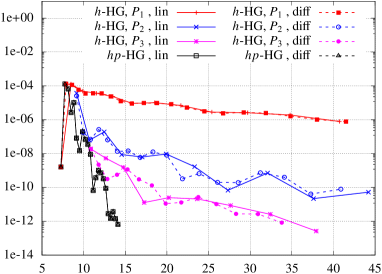
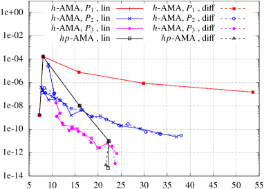
Figure 1: Semilinear problem (43) – (44), comparison of the convergence of the error estimator $|\eta^{\scriptscriptstyle\mathrm{I}}|$ with respect to $\mathrm{DoF}^{1/3}$ for dual problems based on differentiation (45) (“diff”, dashed lines) and linearization (46) (“lin”, full lines) for different adaptive techniques, $h$-HG and $hp$-HG (left) and $h$-AMA and $hp$-AMA (right).

Moreover, the accuracy of the error estimator is demonstrated by Figure 2 where we compare the error $e_{h}:=|J(u)-J({{u}_{h}})|$ with its estimator $|\eta^{\scriptscriptstyle\mathrm{I}}|$ for all adaptive techniques. These values are also given in Tables 1 and 2, where we also show the effectivity index $i_{\mathrm{eff}}:=|\eta^{\scriptscriptstyle\mathrm{I}}|/e_{h}$ and the computational time in seconds. The effectivity indexes are not as close to 1 as would be expected, which is caused by the higher-order reconstruction operator ${{\mathscr{R}}}$ used in (27). Hence, the development of a more accurate reconstruction working on anisotropic $hp$-meshes is still an open problem. However, Figure 2 shows a tight approximation of the error which is not the case for the following examples where the nonlinearities are much stronger. Furthermore, due to the regularity of the exact solution, the higher-order approximations are superior to the low-order methods. The $hp$-HG method achieved the prescribed tolerance using fewer $\mathrm{DoF}$ than $hp$-AMA but it required many more adaptive cycles; hence, the corresponding computational times are comparable. We note that the linearization and algebraic errors ($\approx\eta^{\scriptscriptstyle\mathrm{L}}+\eta^{\scriptscriptstyle\mathrm{A}}+\eta^{\scriptscriptstyle\mathrm{J}}$) in this example is negligible due to the weak nonlinearity and therefore they are not treated.

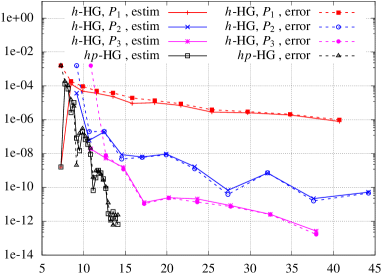
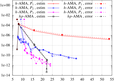
Figure 2: Semilinear problem (43) – (44), convergence of the error $|J(u)-J({{u}_{h}})|$ (“error”, dashed lines) and its estimator $|\eta^{\scriptscriptstyle\mathrm{I}}|$ (“estim”, full lines) with respect to $\mathrm{DoF}^{1/3}$ for different adaptive techniques, $h$-HG and $hp$-HG (left) and $h$-AMA and $hp$-AMA (right).

$h$-HG, $P_{1}$
$\ell$	$\mathrm{DoF}$	$|e_{h}|$	$|\eta^{\scriptscriptstyle\mathrm{I}}|$	$i_{\mathrm{eff}}$	time
0	384	1.58E-03	1.60E-09	0.00	0.3
1	609	1.87E-04	1.29E-04	0.69	0.7
2	969	9.27E-05	4.86E-05	0.52	1.0
3	1545	5.08E-05	3.65E-05	0.72	1.6
4	2472	3.83E-05	2.34E-05	0.61	2.5
5	3966	1.93E-05	9.25E-06	0.48	4.6
6	6369	1.36E-05	1.01E-05	0.74	9.5
7	10194	8.72E-06	6.93E-06	0.80	20.2
8	16377	3.89E-06	2.81E-06	0.72	44.0
9	26196	2.99E-06	2.59E-06	0.87	89.1
10	42135	2.10E-06	1.90E-06	0.91	187.9
11	67461	9.86E-07	7.89E-07	0.80	356.2

$h$-HG, $P_{2}$
$\ell$	$\mathrm{DoF}$	$|e_{h}|$	$|\eta^{\scriptscriptstyle\mathrm{I}}|$	$i_{\mathrm{eff}}$	time
0	768	1.58E-03	3.66E-05	0.02	0.4
1	1218	2.00E-07	6.09E-08	0.30	0.9
2	1938	2.02E-07	1.91E-07	0.94	1.5
3	3090	4.78E-09	8.69E-09	1.82	2.6
4	4944	6.00E-09	6.31E-09	1.05	5.1
5	7896	8.45E-09	9.41E-09	1.11	9.9
6	12702	1.26E-09	1.69E-09	1.34	19.9
7	20406	3.84E-11	6.82E-11	1.77	40.1
8	33042	7.41E-10	7.11E-10	0.96	87.2
9	53202	1.59E-11	2.18E-11	1.38	168.8
10	86376	4.64E-11	5.26E-11	1.13	417.1
$h$-HG, $P_{3}$
$\ell$	$\mathrm{DoF}$	$|e_{h}|$	$|\eta^{\scriptscriptstyle\mathrm{I}}|$	$i_{\mathrm{eff}}$	time
0	1280	1.58E-03	1.88E-08	0.00	0.5
1	2030	8.02E-09	5.33E-09	0.66	1.7
2	3230	1.18E-09	1.52E-09	1.29	3.3
3	5150	1.07E-11	1.28E-11	1.20	6.3
4	8270	2.38E-11	2.48E-11	1.04	14.4
5	13220	1.36E-11	2.09E-11	1.54	26.8
6	21140	7.47E-12	8.51E-12	1.14	54.0
7	34070	2.50E-12	2.58E-12	1.03	100.1
8	54590	1.67E-13	2.64E-13	1.58	177.3

$hp$-HG
$\ell$	$\mathrm{DoF}$	$|e_{h}|$	$|\eta^{\scriptscriptstyle\mathrm{I}}|$	$i_{\mathrm{eff}}$	time
0	384	1.58E-03	1.60E-09	0.00	0.3
1	465	1.83E-04	1.29E-04	0.71	0.5
2	537	1.04E-04	6.55E-05	0.63	0.6
3	612	1.48E-05	2.64E-06	0.18	0.8
4	687	6.31E-06	1.03E-05	1.63	0.9
5	764	2.05E-09	8.19E-08	39.94	1.1
6	860	1.55E-07	1.47E-08	0.10	1.3
7	960	2.95E-07	1.94E-07	0.66	1.5
8	1060	1.03E-07	6.85E-08	0.67	1.8
9	1160	7.23E-08	3.48E-08	0.48	2.2
10	1265	2.10E-08	9.10E-09	0.43	2.6
11	1384	3.95E-10	6.54E-11	0.17	3.0
12	1507	9.39E-10	3.72E-10	0.40	3.6
13	1631	9.21E-10	1.02E-09	1.10	4.2
14	1757	5.90E-10	7.20E-10	1.22	4.8
15	1888	2.69E-10	3.26E-10	1.21	5.6
16	2028	1.07E-10	8.83E-11	0.83	6.5
17	2172	1.22E-11	2.82E-12	0.23	7.5
18	2325	1.04E-12	1.46E-12	1.40	8.7
19	2482	5.93E-13	3.68E-12	6.20	10.3
20	2648	2.25E-12	1.41E-12	0.63	12.0
21	2816	2.35E-12	6.48E-13	0.28	14.0

Table 1: Semilinear problem (43) – (44), error $e_{h}=|J(u)-J({{u}_{h}})|$, its estimate $|\eta^{\scriptscriptstyle\mathrm{I}}|$, effectivity index $i_{\mathrm{eff}}$ and the computational time in seconds for $h$-HG and $hp$-HG adaptive methods.

$h$-AMA, $P_{1}$
$\ell$	$\mathrm{DoF}$	$|e_{h}|$	$|\eta^{\scriptscriptstyle\mathrm{I}}|$	$i_{\mathrm{eff}}$	time
0	384	1.58E-03	1.60E-09	0.00	0.4
1	522	2.17E-04	1.69E-04	0.78	0.6
2	3987	1.19E-05	7.71E-06	0.65	3.3
3	26832	1.40E-06	8.67E-07	0.62	37.8
4	154239	2.16E-07	1.51E-07	0.70	704.7

$h$-AMA, $P_{2}$
$\ell$	$\mathrm{DoF}$	$|e_{h}|$	$|\eta^{\scriptscriptstyle\mathrm{I}}|$	$i_{\mathrm{eff}}$	time
0	768	1.58E-03	3.66E-05	0.02	0.4
1	1218	1.72E-07	3.89E-08	0.23	0.9
2	786	1.81E-07	3.31E-08	0.18	1.1
3	444	6.53E-07	3.94E-07	0.60	1.3
4	480	4.32E-07	2.89E-07	0.67	1.4
5	594	1.74E-07	1.39E-07	0.80	1.6
6	1020	4.38E-08	6.32E-08	1.44	1.9
7	1578	5.70E-08	3.18E-08	0.56	2.4
8	2172	2.39E-08	1.29E-08	0.54	3.1
9	2838	6.50E-10	1.58E-09	2.42	4.1
10	4512	4.16E-09	4.47E-09	1.07	5.9
11	6354	1.15E-09	1.17E-09	1.01	8.8
12	8598	1.27E-09	1.34E-09	1.06	13.3
13	12606	4.24E-10	3.89E-10	0.92	20.7
14	15654	6.99E-11	1.98E-10	2.84	30.8
15	24780	1.23E-10	1.13E-10	0.92	50.2
16	36750	2.94E-11	4.64E-11	1.58	84.5
17	50820	2.46E-11	2.27E-11	0.92	144.6

$h$-AMA, $P_{3}$
$\ell$	$\mathrm{DoF}$	$|e_{h}|$	$|\eta^{\scriptscriptstyle\mathrm{I}}|$	$i_{\mathrm{eff}}$	time
0	1280	1.58E-03	1.88E-08	0.00	0.6
1	1600	2.38E-09	2.37E-09	0.99	1.3
2	1350	8.90E-10	1.32E-09	1.48	1.8
3	1880	3.65E-10	2.41E-10	0.66	2.6
4	2980	3.69E-10	1.68E-10	0.45	3.8
5	3050	2.46E-11	1.10E-10	4.49	5.1
6	3700	4.67E-11	1.09E-10	2.34	6.7
7	4810	2.41E-12	3.76E-11	15.63	9.0
8	6390	2.89E-11	1.69E-11	0.58	12.2
9	7920	1.36E-11	2.54E-12	0.19	16.4
10	10650	2.05E-12	6.41E-12	3.13	24.5
11	13890	1.93E-12	8.24E-13	0.43	33.1
$hp$-AMA
$\ell$	$\mathrm{DoF}$	$|e_{h}|$	$|\eta^{\scriptscriptstyle\mathrm{I}}|$	$i_{\mathrm{eff}}$	time
0	384	1.58E-03	1.60E-09	0.00	0.4
1	522	2.17E-04	1.69E-04	0.78	0.8
2	4086	1.63E-08	1.03E-08	0.63	3.1
3	11162	1.43E-11	9.93E-12	0.69	10.0
4	10850	2.08E-13	4.82E-14	0.23	17.5

Table 2: Semilinear problem (43) – (44), error $e_{h}=|J(u)-J({{u}_{h}})|$, its estimate $|\eta^{\scriptscriptstyle\mathrm{I}}|$, effectivity index $i_{\mathrm{eff}}$ and the computational time in seconds for $h$-AMA and $hp$-AMA adaptive methods.

5.2 Quasilinear elliptic problem on L-shaped domain

Similarly as in [29], we consider a quasilinear elliptic problem on L-shaped domain ${\Omega}:=(-1,1)^{2}\setminus[0,1)\times(-1,0]$

$$-\nabla\cdot(\mu(|\nabla u|)\nabla u) =f\qquad\hskip 7.0pt\mbox{ in }{\Omega},$$ (47)

where $\mu(|\nabla u|)=1+\exp(-|\nabla u|^{2})$ is a nonlinear diffusion. We prescribe the Dirichlet boundary condition on the boundary $\partial{\Omega}$ and the function $f$ such that the exact solution is $u=r^{2/3}\sin(2\phi/3)$ with $(r,\phi)$ being the polar coordinates. The target functional represents the total energy (cf. (57) in Section 5.4) in a small polygonal domain around the interior corner ${\Omega}_{B}:=\{(x_{1},x_{2})\in{\Omega},\ |x_{i}|\leq 0.05,\ i=1,2\}$; i.e.,

$$J(u)=\int\nolimits_{{\Omega}_{B}}\mu(|\nabla u|)|\nabla u|^{2}{\,\mathrm{d}x}.$$ (48)

Since the exact solution is know, the reference value $J(u)=1.721609238808\cdot 10^{-2}$ has been computed using a numerical quadrature. Figure 3, left, shows the primal and adjoint solutions corresponding to (47)–(48) together with the domain of interest ${\Omega}_{B}$. Due to the interior angle the primal and adjoint solutions have a singularity.

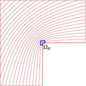
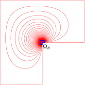
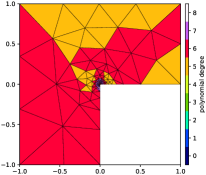
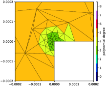
Figure 3: Quasilinear elliptic problem (47)–(48): primal solution (first), adjoint solution (second), and the final $hp$-mesh (third) and its 5000x zoom near the interior corner (last).

We solve this problem only by the $hp$-AMA adaptive technique. Figure 4, left, shows the convergence of the error $e_{h}:=|J(u)-J({{u}_{h}})|$ and the various parts of the error estimator: linearization $|\eta^{\scriptscriptstyle\mathrm{L}}|$ and $|\eta^{\scriptscriptstyle\mathrm{J}}|$, residual $|\eta^{\scriptscriptstyle\mathrm{S}}|$, and algebraic $|\eta^{\scriptscriptstyle\mathrm{A}}|$ with respect to $\mathrm{DoF}^{1/3}$, cf. (2.4); each node corresponds to one level of mesh adaptation. Moreover, Table 3 shows the vales of $e_{h}$, $|\eta^{\scriptscriptstyle\mathrm{I}}|$, the effectivity index $i_{\mathrm{eff}}:=|\eta^{\scriptscriptstyle\mathrm{I}}|/e_{h}$ and the computational time in seconds. As we do not have an upper bound of the error, it is underestimated at most by a factor of 10. The dominating term is the residual estimator $|\eta^{\scriptscriptstyle\mathrm{S}}|$. The convergence of all estimators is not monotone, which is a typical behaviour for anisotropic adaptation. Nevertheless, an exponential rate of convergence is observed. The prescribed tolerance $\mathrm{TOL}=10^{-10}$ is achieved after 21 levels of mesh adaptation.

Moreover, Figure 4, right, shows the convergence of the nonlinear solver level $\ell=0,1,\dots,21$ of mesh adaptation. Particularly, we plot both sides of the stopping criterion (40), i.e., the estimate of the algebraic error $|\eta^{\scriptscriptstyle\mathrm{A}}({{u}_{h,\ell}^{(k)}},{{z}_{h,\ell}^{(k)}})|$ and the adaptively chosen tolerance ${C_{{A}}}|\eta^{\scriptscriptstyle\mathrm{S}}|$ (with ${C_{{A}}}=0.1$). Each node corresponds to one nonlinear iteration $k=0,1,\dots$, but on different adaptive level $\ell=0,1,\dots$, in general. The black left-right arrows indicates one mesh adaptive loop $\ell$. We observe that the algebraic error tolerance ${C_{{A}}}|\eta^{\scriptscriptstyle\mathrm{S}}|$ only requires recalculation at most once within one mesh adaptive level (for $\ell=2,6,7,11,13,15,16,19$). Further, this tolerance is step by step decreasing (but not, in general, monotonic) when the total error estimates $|\eta^{\scriptscriptstyle\mathrm{I}}|=|\eta^{\scriptscriptstyle\mathrm{S}}+\eta^{\scriptscriptstyle\mathrm{A}}+\eta^{\scriptscriptstyle\mathrm{L}}+\eta^{\scriptscriptstyle\mathrm{J}}|$ is approaching to the tolerance $\mathrm{TOL}$.

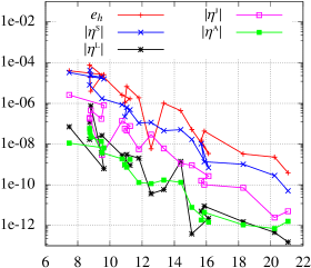
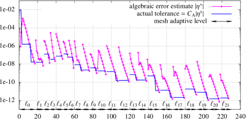
Figure 4: Quasilinear elliptic problem (47)–(48), convergence of $e_{h}=|J(u)-J({{u}_{h}})|$ and its estimators $|\eta^{\scriptscriptstyle\mathrm{S}}|$, $|\eta^{\scriptscriptstyle\mathrm{L}}|$, $|\eta^{\scriptscriptstyle\mathrm{J}}|$ and $|\eta^{\scriptscriptstyle\mathrm{A}}|$ with respect to $\mathrm{DoF}^{1/3}$ (left) and the convergence of the nonlinear iterative solver for adaptive levels $\ell=0,\dots 21$.

$hp$-AMA
$\ell$	$\mathrm{DoF}$	$|e_{h}|$	$|\eta^{\scriptscriptstyle\mathrm{I}}|$	$i_{\mathrm{eff}}$	time
0	417	3.97E-05	3.26E-05	0.82	0.9
1	891	2.56E-05	1.58E-05	0.62	1.9
2	849	2.14E-05	1.90E-05	0.89	3.5
3	684	3.92E-06	2.35E-05	5.99	4.4
4	671	1.93E-05	4.24E-05	2.19	5.4
5	668	7.48E-05	8.06E-06	0.11	6.7
6	859	2.37E-05	1.72E-06	0.07	8.7
7	1244	2.53E-06	8.58E-07	0.34	12.0

$hp$-AMA
$\ell$	$\mathrm{DoF}$	$|e_{h}|$	$|\eta^{\scriptscriptstyle\mathrm{I}}|$	$i_{\mathrm{eff}}$	time
8	1425	1.68E-06	4.84E-07	0.29	14.5
9	1303	1.09E-06	2.22E-07	0.20	19.0
10	1346	6.70E-06	6.29E-07	0.09	23.2
11	1642	1.86E-06	1.09E-07	0.06	28.7
12	1982	5.86E-09	1.16E-07	19.82	33.8
13	2379	1.02E-06	4.54E-08	0.04	44.1
14	2987	4.32E-07	5.07E-08	0.12	55.4
15	3438	5.15E-08	1.67E-08	0.32	79.3

$hp$-AMA
$\ell$	$\mathrm{DoF}$	$|e_{h}|$	$|\eta^{\scriptscriptstyle\mathrm{I}}|$	$i_{\mathrm{eff}}$	time
16	4193	3.40E-09	6.84E-10	0.20	116.2
17	3851	1.55E-08	1.03E-08	0.67	144.0
18	3993	4.34E-08	1.35E-09	0.03	186.0
19	6111	3.25E-09	1.01E-09	0.31	252.0
20	8278	2.26E-09	2.83E-10	0.13	317.7
21	9348	3.85E-10	5.01E-11	0.13	412.2

Table 3: Quasilinear elliptic problem (47)–(48), error $e_{h}=|J(u)-J({{u}_{h}})|$, its estimate $|\eta^{\scriptscriptstyle\mathrm{I}}|$, effectivity index $i_{\mathrm{eff}}$ and the computational time in seconds obtained by $hp$-AMA adaptive method for adaptive levels $\ell=0,\dots 21$.

The resulting $hp$-grid with detail near the interior corner is shown in Figure 3, right. The large elements with high polynomial degrees are outside of the singularity; whereas, small elements with a low polynomial degree ($p=3$) are generated near the interior corner.

5.3 Convective-dominated problem with the Carreau-law diffusion

We consider the convection-diffusion problem in the form

$$-\nabla\cdot(\mu(|\nabla u|)\nabla u)+\bm{b}\cdot\nabla u=0\qquad\mbox{ in }{\Omega}:=(0,2)\times(0,1),$$ (49)

where $\bm{b}=(x_{2},(1-x_{1})^{2})$ is the prescribed velocity field and the nonlinear diffusion is given by the Carreau law for a non-Newtonian fluid ([4, 7, 9])

$$\mu(|\nabla u|)=\varepsilon(k_{\infty}+(k_{0}-k_{\infty}))\left(1+\lambda|\nabla u|^{2}\right)^{(\theta-2)/\theta},$$ (50)

where $\varepsilon>0$, $\lambda>0$, $1<\theta\leq 2$ and $0<k_{\infty}<k_{0}$ . We prescribe the homogeneous Neumann data at the outflow part ${\Gamma}_{N}:=\{2\}\times(0,1)\cup(0,2)\times\{1\}$ and the discontinuous Dirichlet data

$$u=\left\{\begin{array}[]{ll}1&x_{1}\in(\frac{1}{8},\frac{1}{2}),\ x_{2}=0\\[2.0pt] 2&x_{1}\in(\frac{1}{2},\frac{3}{4}),\ x_{2}=0\\[2.0pt] 0&\mbox{ elsewhere on }{\Gamma}_{D}:={\Gamma}\setminus{\Gamma}_{N}.\end{array}\right.$$ (51)

We consider the values $\varepsilon=10^{-4}$, $\lambda=1$, $\theta=1.2$, $k_{\infty}=1$ and $k_{0}=2$. The discontinuity of the boundary conditions leads to the presence of three interior layers which propagates through the computational domain and which are smeared due to the presence of diffusion.

The quantity of interest is given by the integral $J(u)=\int_{\Gamma_{B}}u{\,\mathrm{d}S}$, where $\Gamma_{B}:=\{(x_{1},x_{2}),\ 1.8<x_{1}<2,\ x_{2}=1\}\cup\{(x_{1},x_{2}),\ x_{1}=1,\ 0.8<x_{2}<1\}$ is a part of the Neumann boundary ${\Gamma}_{N}$. The reference value obtain by computations obtained on a strongly refined grid is $0.280006172$. We solved this problem with the $hp$-AMA method where the error tolerance is $\mathrm{TOL}=10^{-10}$.

Figure 5, left, shows the convergence of the error $e_{h}=|J(u)-J({{u}_{h}})|$ and the various parts of the error estimator: linearization $|\eta^{\scriptscriptstyle\mathrm{L}}|$, residual $|\eta^{\scriptscriptstyle\mathrm{S}}|$ and algebraic $|\eta^{\scriptscriptstyle\mathrm{A}}|$ with respect to $\mathrm{DoF}^{1/3}$, cf. (2.4); each node corresponds to one level of mesh adaptation. Here, $\eta^{\scriptscriptstyle\mathrm{J}}=0$. The values $e_{h}$, $\eta^{\scriptscriptstyle\mathrm{I}}$, effectivity index $i_{\mathrm{eff}}$ and computational time are shown in Table 4. We observe the exponential rate of the convergence and a reasonable approximation of the error, about $0.1\lesssim i_{\mathrm{eff}}\lesssim 10$ due to a strong anisotropy of the meshes. It is obvious namely for the last two levels of adaption where the limits of finite precision arithmetic and the error in the reference value for the quantity of interest, obtained by a highly refined mesh approximation, may both play non-negligible roles. The dominant part of the estimator is $|\eta^{\scriptscriptstyle\mathrm{S}}|$; however, the role of the estimator $|\eta^{\scriptscriptstyle\mathrm{L}}|$ is larger in comparison to previous examples.

Moreover, Figure 5, right, shows the convergence of the nonlinear solver for each mesh adaptation level $\ell=0,1,\dots,26$. Again, we plot both sides of the stopping criterion (40), the algebraic estimate $|\eta^{\scriptscriptstyle\mathrm{A}}({{u}_{h,\ell}^{(k)}},{{z}_{h,\ell}^{(k)}})|$ and the adaptively chosen tolerance ${C_{{A}}}|\eta^{\scriptscriptstyle\mathrm{S}}|$ (with ${C_{{A}}}=0.1$). Each node corresponds to one nonlinear iteration $k=0,1,\dots$ but on a different adaptive level $\ell=0,1,\dots$, in general. The black left-right arrows indicates one mesh adaptive loop $\ell$. A step by step decrease of the error tolerance and the convergence of the nonlinear solver is obvious.

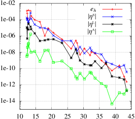
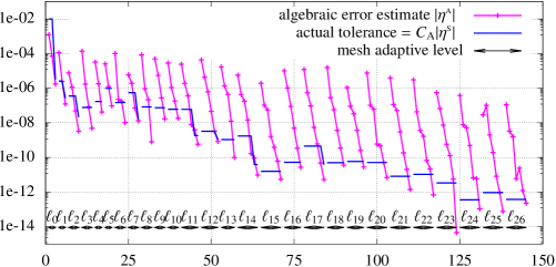
Figure 5: Convection with the Carreau law diffusion (49)–(51), convergence of the error $e_{h}=|J(u)-J(u_{h})|$ and its estimators $|\eta^{\scriptscriptstyle\mathrm{S}}|$, $|\eta^{\scriptscriptstyle\mathrm{L}}|$ and $|\eta^{\scriptscriptstyle\mathrm{A}}|$ with respect to $\mathrm{DoF}^{1/3}$ (left) and the convergence of the nonlinear iterative solver for adaptive levels $\ell=0,1,\dots,26$.

$hp$-AMA
$\ell$	$\mathrm{DoF}$	$|e_{h}|$	$|\eta^{\scriptscriptstyle\mathrm{I}}|$	$i_{\mathrm{eff}}$	time
0	2400	1.20E-03	6.87E-04	0.57	2.3
1	2064	1.46E-03	4.04E-05	0.03	4.1
2	1833	1.23E-03	1.68E-04	0.14	5.8
3	1881	5.90E-04	1.17E-04	0.20	7.2
4	1908	1.70E-04	1.04E-04	0.61	8.5
5	2033	4.23E-05	5.61E-05	1.33	9.9
6	2493	3.05E-04	1.39E-04	0.46	11.8
7	3177	9.51E-05	2.55E-05	0.27	15.0
8	4360	5.51E-05	1.07E-05	0.19	18.6
9	5702	9.94E-07	9.38E-06	9.44	23.6

$hp$-AMA
$\ell$	$\mathrm{DoF}$	$|e_{h}|$	$|\eta^{\scriptscriptstyle\mathrm{I}}|$	$i_{\mathrm{eff}}$	time
10	6773	9.05E-06	6.07E-06	0.67	30.0
11	8684	2.51E-06	1.14E-06	0.45	42.3
12	12574	3.97E-07	2.55E-07	0.64	63.7
13	17848	2.67E-08	2.54E-07	9.51	88.4
14	21028	2.82E-07	2.85E-08	0.10	143.9
15	21948	1.39E-07	1.53E-08	0.11	187.0
16	24134	4.96E-09	4.55E-08	9.18	234.0
17	27754	2.93E-08	7.62E-09	0.26	324.1
18	32985	4.25E-09	3.62E-08	8.52	393.0
19	34260	1.09E-08	1.62E-08	1.48	471.5

$hp$-AMA
$\ell$	$\mathrm{DoF}$	$|e_{h}|$	$|\eta^{\scriptscriptstyle\mathrm{I}}|$	$i_{\mathrm{eff}}$	time
20	37989	7.22E-09	8.13E-09	1.13	569.4
21	45251	9.66E-10	5.55E-09	5.74	697.0
22	50881	3.28E-10	7.10E-10	2.16	853.0
23	58855	5.53E-11	3.68E-10	6.65	1048.0
24	70198	2.45E-10	1.47E-10	0.60	1309.4
25	77932	1.05E-11	2.64E-10	25.23	1646.3
26	82447	2.36E-12	3.83E-11	16.25	2058.4

Table 4: Convection with the Carreau law diffusion (49)–(51), error $e_{h}=|J(u)-J({{u}_{h}})|$, its estimate $|\eta^{\scriptscriptstyle\mathrm{I}}|$, effectivity index $i_{\mathrm{eff}}$ and the computational time in seconds obtained by $hp$-AMA adaptive method for adaptive levels $\ell=0,\dots 26$.

Finally, Figure 6 shows the resulting $hp$-grid and the corresponding solution. A mesh alignment of anisotropic elements along the interior layers is obvious; the lowest polynomial degree and larger mesh elements are generated outside of these layers, where the solution is almost constant.

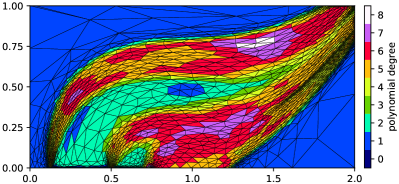
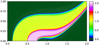
Figure 6: Convection with the Carreau law diffusion (49)–(51), final $hp$-mesh (left) and the solution (right) obtained by $hp$-AMA method.

5.4 Magneto-static field of an alternator

The last example follows from [23] where the magnetic state in the cross-section of an alternator was solved numerically. Due to the symmetry, only one quarter of the alternator is taken as the computational domain ${\Omega}:={\Omega}_{s}\cup{\Omega}_{s}\cup{\Omega}_{a}$; see Figure 7, left, where the geometry of the domain is shown. The alternator consists of the stator ($\Omega_{s}$) and rotor ($\Omega_{r}$) with a gap filled by air ($\Omega_{a}$).

The problem is described by the Maxwell equations for the stationary magnetic field in the form

$$\operatorname*{rot}H =f\qquad\mbox{in }{\Omega},$$ (52a)

$$\operatorname*{div}B =0\qquad\mbox{in }{\Omega},$$ (52b)

where $H=(H_{1},H_{2})$ is the magnetic intensity field, $B=(B_{1},B_{2})$ is the magnetic induction field and $f$ is the current density (its component perpendicular to the plane of the computational domain). The differential operators appearing in (52) are given by $\operatorname*{rot}H=(\partial H_{2}/\partial x_{1},\,\partial H_{1}/\partial x_{2})$ and $\operatorname*{div}B=\nabla\cdot B=\partial B_{1}/\partial x_{1}+\partial B_{2}/\partial x_{2}$ in two space dimensions.

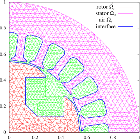
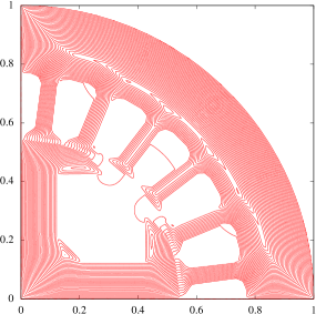
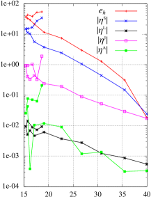
Figure 7: Alternator, the computational domain with its components together with the initial mesh (left), the isolines of the primal solution (center) and the convergence of $e_{h}=|J(u)-J({{u}_{h}})|$ and its estimators $|\eta^{\scriptscriptstyle\mathrm{S}}|$, $|\eta^{\scriptscriptstyle\mathrm{L}}|$, $|\eta^{\scriptscriptstyle\mathrm{J}}|$ and $|\eta^{\scriptscriptstyle\mathrm{A}}|$ with respect to $\mathrm{DoF}^{1/3}$ (right).

$hp$-AMA
$\ell$	$\mathrm{DoF}$	$|e_{h}|$	$|\eta^{\scriptscriptstyle\mathrm{I}}|$	$i_{\mathrm{eff}}$	time
0	6462	5.45E+01	3.46E+01	0.63	313.5
1	5487	5.31E+01	2.71E+01	0.51	401.6
2	4648	3.87E+01	1.68E+01	0.43	501.4
3	3913	4.33E+01	1.54E+01	0.35	567.6
4	3617	3.72E+01	1.50E+01	0.40	603.3

$hp$-AMA
$\ell$	$\mathrm{DoF}$	$|e_{h}|$	$|\eta^{\scriptscriptstyle\mathrm{I}}|$	$i_{\mathrm{eff}}$	time
5	3883	3.34E+01	1.13E+01	0.34	678.7
6	4261	2.94E+01	1.04E+01	0.35	737.0
7	5010	2.15E+01	5.63E+00	0.26	819.0
8	6942	1.16E+01	3.77E+00	0.32	960.6
9	11597	7.43E+00	2.44E+00	0.33	1224.0

$hp$-AMA
$\ell$	$\mathrm{DoF}$	$|e_{h}|$	$|\eta^{\scriptscriptstyle\mathrm{I}}|$	$i_{\mathrm{eff}}$	time
10	19107	2.97E+00	1.06E+00	0.35	1717.4
11	29004	1.29E+00	4.42E-01	0.34	2604.6
12	44588	3.13E-01	1.48E-01	0.47	4210.5
13	63867	1.81E-02	2.43E-02	1.34	8961.9

Table 5: Alternator, error $e_{h}=|J(u)-J({{u}_{h}})|$, its estimate $|\eta^{\scriptscriptstyle\mathrm{I}}|$, effectivity index $i_{\mathrm{eff}}$ and the computational time in seconds obtained by $hp$-AMA adaptive method for adaptive levels $\ell=0,\dots 13$.

Moreover, we consider the constitutive relation

$$H(x)=\nu(x,|B(x)|^{2})B(x),\quad x\in{\Omega},$$ (53)

where

$$\nu(x,r)=\begin{cases}\frac{1}{\mu_{0}}&\mbox{ for }x\in{\Omega}_{a},\\ \frac{1}{\mu_{0}}\left(\alpha+(1-\alpha)\frac{r^{4}}{\beta+r^{4}}\right)&\mbox{ for }x\in{\Omega}_{s}\cup{\Omega}_{r}.\\ \end{cases}$$ (54)

The symbol $\mu_{0}=1.256\times 10^{-6}\,\mathrm{kg}\cdot\mathrm{m}\cdot\mathrm{A}^{-2}\cdot\mathrm{s}^{-2}$ denotes the permeability of the vacuum and the material coefficients are $\alpha=0.0003$, $\beta=16000$ according to [23]. We consider the constant current density $f=5\times 10^{4}\,\mathrm{A}\cdot\mathrm{m}^{-2}$.

Assuming that there exists a potential $u:{\Omega}\to\mathbb{R}$ such that $B=\operatorname*{curl}u=(\partial u/\partial x_{2},-\partial u/\partial x_{1})$, equation (52b) is satisfied directly. Obviously, $|B|=|\nabla u|$ and, therefore, (52a) together with (53) gives

$$f=\operatorname*{rot}H=\operatorname*{rot}\nu(x,|B(x)|^{2})B(x)=\operatorname*{rot}\nu(x,|\nabla u(x)|^{2})\operatorname*{curl}u(x)=-\nabla\cdot\left(\nu(x,|\nabla u(x)|^{2})\nabla u\right).$$ (55)

Consequently, we have the following problem. Find $u:{\Omega}\to\mathbb{R}$ such that

$$-\nabla\cdot\left(\nu(x,|\nabla u(x)|^{2})\nabla u\right) =f\qquad\mbox{ in }{\Omega}.$$ (56)

The homogeneous Dirichlet boundary condition is prescribed on $\Gamma$ for simplicity as in [23], but other options are possible. We are interested in the total magnetic energy; hence, the target quantity is given by

$$E=\frac{1}{2}\int_{{\Omega}}H(x)\cdot B(x){\,\mathrm{d}x}=\frac{1}{2}\int_{{\Omega}}\nu(x,|B(x)|^{2})|B(x)|^{2}{\,\mathrm{d}x}=\frac{1}{2}\int_{{\Omega}}\nu(x,|\nabla u(x)|^{2})|\nabla u(x)|^{2}{\,\mathrm{d}x}=:J(u).$$ (57)

Figure 7, center, shows the corresponding isolines of the primal solution obtained on a fine grid where we obtained the reference value $J(u)=2\,664\,\mathrm{kg}\cdot\mathrm{m}^{2}\cdot\mathrm{s}^{-2}$.

We solve this problem with the $hp$-AMA technique. Since function $\nu$ given by (54) differs for several orders, the mesh adaptation technique must maintain the material interfaces. Figure 7, right, shows the convergence of the error $e_{h}=|J(u)-J({{u}_{h}})|$ and the error estimators $|\eta^{\scriptscriptstyle\mathrm{L}}|$, $|\eta^{\scriptscriptstyle\mathrm{J}}|$, $|\eta^{\scriptscriptstyle\mathrm{S}}|$ and $|\eta^{\scriptscriptstyle\mathrm{A}}|$ with respect to $\mathrm{DoF}^{1/3}$, cf. (2.4). The values $e_{h}$, $\eta^{\scriptscriptstyle\mathrm{I}}$, effectivity index $i_{\mathrm{eff}}$ and computational time are shown in Table 5. Again, we observe a reasonable approximation of the error and the exponential rate of the convergence. The final $hp$-grid and primal solution are plotted in Figure 8. A strong refinement along the material interfaces is obvious.

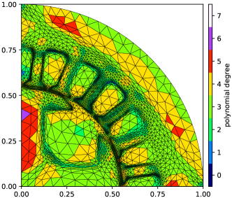
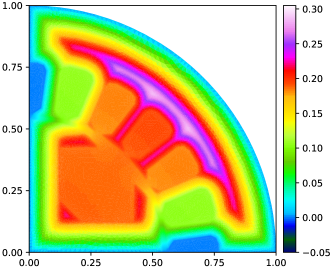
Figure 8: Alternator, the final $hp$-mesh (left) and the corresponding magnetic potential (right).

6 Conclusion

We presented the framework of the goal-oriented error estimates for nonlinear problems where the adjoint solution is based on the linearization of the primal weak formulation used in the iterative solution of the corresponding algebraic systems. We derived abstract error estimates consisting of three ingredients: dual weighted residual, algebraic error and error arising from the linearization. Then, employing a higher-order reconstruction, we proposed computable error estimates and an adaptive algorithm for the numerical solution of nonlinear PDEs. The presented numerical experiments demonstrate a reasonable approximation of the error of the quantity of interest and also an exponential rate of convergence of the $hp$-adaptive method. We are aware that the effectivity indexes are not enough close to the desired value around 1 but this is caused by an insufficient accuracy of the higher order approximation of the exact solutions of primal and dual problems on $hp$-anisotropic meshes. Nevertheless, the presented examples demonstrate a benefit of the use of such meshes. An improvement of the higher-order reconstruction will be a subject of further research.

References

- [1] Babuška, I., Suri, M.: The - and - versions of the finite element method. An overview. Comput. Methods Appl. Mech. Engrg. 80, 5–26 (1990)
- [2] Balan, A., Woopen, M., May, G.: Adjoint-based -adaptivity on anisotropic meshes for high-order compressible flow simulations. Comput. Fluids 139, 47 – 67 (2016)
- [3] Bangerth, W., Rannacher, R.: Adaptive Finite Element Methods for Differential Equations. Lectures in Mathematics. ETH Zürich. Birkhäuser Verlag (2003)
- [4] Barrett, J., Liu, W.: Finite element error analysis of a quasi-Newtonian flow obeying the Carreau or power law. Numer. Math. 64(1), 433–453 (1993)
- [5] Becker, R., Brunner, M., Innerberger, M., Melenk, J.M., Praetorius, D.: Rate-optimal goal-oriented adaptive FEM for semilinear elliptic PDEs. Comput. Math. Appl. 118, 18–35 (2022)
- [6] Becker, R., Rannacher, R.: An optimal control approach to a-posteriori error estimation in finite element methods. Acta Numerica 10, 1–102 (2001)
- [7] Berrone, S., Süli, E.: Two-sided a posteriori error bounds for incompressible quasi-Newtonian flows. IMA J. Numer. Anal. 28(2), 382–421 (2008)
- [8] Chaillou, A., Suri, M.: Computable error estimators for the approximation of nonlinear problems by linearized models. Comput. Methods Appl. Mech. Engrg. 196(1-3), 210–224 (2006)
- [9] Congreve, S., Houston, P., Süli, E., Wihler, T.: Discontinuous Galerkin finite element approximation of quasilinear elliptic boundary value problems II: Strongly monotone quasi-Newtonian flows. IMA J. Numer. Anal. 33(4), 1386–1415 (2013)
- [10] Congreve, S., Wihler, T.P.: Iterative Galerkin discretizations for strongly monotone problems. J. Comput. Appl. Math. 311, 457 – 472 (2017)
- [11] Demkowicz, L., Rachowicz, W., Devloo, P.: A fully automatic -adaptivity. J. Sci. Comput. 17(1-4), 117–142 (2002)
- [12] Di Stolfo, P., Rademacher, A., Schröder, A.: Dual weighted residual error estimation for the finite cell method. Journal of Numerical Mathematics 27(2), 101–122 (2019)
- [13] Dolejší, V., Bartoš, O., Roskovec, F.: Goal-oriented mesh adaptation method for nonlinear problems including algebraic errors. Comput. Math. Appl. 93, 178–198 (2021)
- [14] Dolejší, V., Feistauer, M.: Discontinuous Galerkin Method – Analysis and Applications to Compressible Flow. Springer Series in Computational Mathematics 48. Springer, Cham (2015)
- [15] Dolejší, V., May, G.: Anisotropic -Mesh Adaptation Methods. Birkhäuser (2022)
- [16] Dolejší, V., May, G., Roskovec, F., Solin, P.: Anisotropic -mesh optimization technique based on the continuous mesh and error models. Comput. Math. Appl. 74, 45–63 (2017)
- [17] Dolejší, V., Solin, P.: -discontinuous Galerkin method based on local higher order reconstruction. Appl. Math. Comput. 279, 219–235 (2016)
- [18] Dolejší, V., Tichý, P.: On efficient numerical solution of linear algebraic systems arising in goal-oriented error estimates. Journal of Scientific Computing 83(5) (2020)
- [19] Endtmayer, B., Langer, U., Wick, T.: Two-side a posteriori error estimates for the dual-weighted residual method. SIAM Journal on Scientific Computing 42(1), A371–A394 (2020)
- [20] Ern, A., Vohralík, M.: Adaptive inexact Newton methods with a posteriori stopping criteria for nonlinear diffusion PDEs. SIAM J. Sci. Comput. 35(4), A1761–A1791 (2013)
- [21] Fidkowski, K., Darmofal, D.: Review of output-based error estimation and mesh adaptation in computational fluid dynamics. AIAA Journal 49(4), 673–694 (2011)
- [22] Giles, M., Süli, E.: Adjoint methods for PDEs: a posteriori error analysis and postprocessing by duality. Acta Numerica 11, 145–236 (2002)
- [23] Glowinski, R., Marrocco, A.: Analyse numérique du champ magnetique d’un alternateur par elements finis et sur-relaxation ponctuelle non lineaire. Comput. Methods Appl. Mech. Engrg. 3, 55–85 (1974)
- [24] Haberl, A., Praetorius, D., Schimanko, S., Vohralik, M.: Convergence and quasi-optimal cost of adaptive algorithms for nonlinear operators including iterative linearization and algebraic solver. Numer. Math. 147(3), 679–725 (2021)
- [25] Hartmann, R.: Adjoint Consistency Analysis of Discontinuous Galerkin Discretizations. SIAM J. Numer. Anal. 45(6), 2671–2696 (2007)
- [26] Hartmann, R., Houston, P.: Symmetric interior penalty DG methods for the compressible Navier-Stokes equations II: Goal-oriented a posteriori error estimation. Int. J. Numer. Anal. Model. 3, 141–162 (2006)
- [27] Heid, P., Praetorius, D., Wihler, T.P.: Energy contraction and optimal convergence of adaptive iterative linearized finite element methods. Comput. Meth. Aappl. Math. 21(2, SI), 407–422 (2021)
- [28] Heid, P., Wihler, T.: On the convergence of adaptive iterative linearized Galerkin methods. Calcolo 57(3) (2020)
- [29] Houston, P., Robson, J., Süli, E.: Discontinuous Galerkin finite element approximation of quasilinear elliptic boundary value problems I: The scalar case. IMA J. Numer. Anal. 25, 726–749 (2005)
- [30] List, F., Radu, F.A.: A study on iterative methods for solving Richards’ equation. Comput. Geosci. 20(2), 341–353 (2016)
- [31] Loseille, A., Alauzet, F.: Continuous mesh framework part I: well-posed continuous interpolation error. SIAM J. Numer. Anal. 49(1), 38–60 (2011)
- [32] Loseille, A., Dervieux, A., Alauzet, F.: Fully anisotropic goal-oriented mesh adaptation for 3D steady Euler equations. J. Comput. Phys. 229(8), 2866–2897 (2010)
- [33] Makridakis, C., Nochetto, R.H.: Elliptic reconstruction and a posteriori error estimates for parabolic problems. SIAM J. Numer. Anal. 41(4), 1585–1594 (2003)
- [34] Mallik, G., Vohralík, M., Yousef, S.: Goal-oriented a posteriori error estimation for conforming and nonconforming approximations with inexact solvers. Journal of Computational and Applied Mathematics 366 (2020)
- [35] Radu, F.A., Nordbotten, J.M., Pop, I.S., Kumar, K.: A robust linearization scheme for finite volume based discretizations for simulation of two-phase flow in porous media. J. Comput. Appl. Math. 289, 134–141 (2015)
- [36] Rannacher, R., Vihharev, J.: Adaptive finite element analysis of nonlinear problems: Balancing of discretization and iteration errors. J. Numer. Math. 21(1), 23–61 (2013)
- [37] Richter, T., Wick, T.: Variational localizations of the dual weighted residual estimator. J. Comput. Appl. Math. 279, 192 – 208 (2015)
- [38] Schwab, C.: - and -Finite Element Methods. Clarendon Press, Oxford (1998)
- [39] Šolín, P., Demkowicz, L.: Goal-oriented -adaptivity for elliptic problems. Comput. Methods Appl. Mech. Engrg. 193, 449–468 (2004)
- [40] Zeidler, E.: Nonlinear functional analysis and its applications. II/B, Nonlinear monotone operators. New York, Springer (1985)