Autoencoder-based Joint Communication and Sensing of Multiple Targets

Abstract

We investigate the potential of autoencoders for building a joint communication and sensing (JCAS) system that enables communication with one user while detecting multiple radar targets and estimating their positions. Foremost, we develop a suitable encoding scheme for the training of the AE and for targeting a fixed false alarm rate of the target detection during training. We compare this encoding with the classification approach using one-hot encoding for radar target detection. Furthermore, we propose a new training method that complies with possible ambiguities in the target locations. We consider different options for training the detection of multiple targets. We can show that our proposed approach based on permuting and sorting can enhance the angle estimation performance so that single snapshot estimations with a low standard deviation become possible. We outperform an Estimation of Signal Parameter via Rotational Invariance Techniques (ESPRIT) benchmark for small numbers of measurement samples.

I Introduction

Electromagnetic sensing and radio communications remain vital services for society, yet an increase in their sustainability, and consequently in their efficiency, is of rising importance. We can increase spectral and energy efficiency by combining radio communication and sensing into one waveform compared to operating two separate systems. Therefore, this work focuses on the codesign of both functionalities in a JCAS system. So far, standardized approaches for localization and communication, such as the LTE Positioning Protocol (LPP), or the New Radio Positioning protocol A (NRPPa), need the cooperation of the user equipment to localize it. The future 6G network is envisioned to natively support JCAS by extending sensing capabilities to non-cooperating targets, such as objects without communication capabilities, and performing general sensing of the surroundings [1]. From this approach, we expect to increase spectral efficiency by making spectral resources accessible to communication while maintaining their use for sensing. Simultaneously, we predict an increase in energy efficiency because of the dual-use of a joint waveform.

In the radar community, the integration of communication capabilities into sensing signals to enhance a standard radar signal with an information sequence for a possible receiver has already been studied [2]. A well-studied approach to combined communication and sensing is OFDM radar [3, 4]. OFDM radar enables the robust detection of objects while maintaining its communication capabilities through careful signal processing. However, there is a growing interest in data-driven approaches based on machine learning (ML) since they can overcome deficits that model-based techniques as used in OFDM face. Especially at higher frequencies used for sensing applications, which will become more important in 6G, these deficits become more pronounced because of hardware imperfections [5]. ML is expected to be prevalent in 6G since its use has matured in communication as well as in radar processing [1]. AE have been studied for communication systems, e.g., [6, 7], and in the context of radar [8, 9]. In [5], an AE for JCAS in a single-carrier system has been proposed and has shown to robustly perform close to a maximum a-posteriori ratio test detector benchmark for single snapshot evaluation and one possible radar target.

In this paper, we explore the monostatic sensing capabilities of a wireless single-carrier communication system. We use an AE approach and study the influence of multi-target sensing and multi-snapshot sensing on the overall performance. This work extends the AE model of [5] by adding multiple target capabilities for detection and localization. We describe the detection of multiple targets not as a classification task with the number of targets as classes but instead design it as parallel detection tasks resulting in the novel counting encoding. The permutation invariance of targets during detection brings additional challenges to the training of the neural networks. To address this issue, we present multiple approaches with low additional complexity.

II System Model

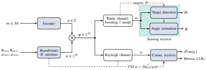
Figure 1: JCAS autoencoder as proposed in [5], light blue blocks are trainable NNs, red dashed paths are only active while propagating the training data

The system block diagram, shown in Fig. 1, is based on [5]. The encoder transforms the data symbols $m\nobreak\in\nobreak\mathcal{M}:=\nobreak\{1,2,\ldots,M\}$ into complex modulation symbols $x\in\mathcal{C}\subset\mathbb{C}$, with $|\mathcal{C}|=M$. The complex symbols are multiplied with a unique $\nu_{i}=g_{i}\exp(\mathrm{j}\gamma_{i})$ for each antenna $i$ with beamforming gain $g_{i}$ and phase shift $\gamma_{i}$ to steer the signal to our areas of interest. The encoder and beamformer employ power normalization to fulfill power constraints. We consider a maximum of $T_{\max}$ radar targets and a linear array of $K$ antennas in the transmitter and the radar receiver. The beamformer inputs are the azimuth angle regions in which communication and sensing should take place. The communication receiver is situated randomly in the interval $[\varphi_{\min},\varphi_{\max}]$ and the radar target positions are uniformly drawn from $[\theta_{\min},\theta_{\max}]$. The transmit signal $\boldsymbol{y}$ is fed into a Rayleigh channel before being received by the communication receiver with a single antenna as

$$z_{\text{c}}=\beta\boldsymbol{a}_{\text{TX}}(\varphi)^{\top}\boldsymbol{y}+n,$$ (1)

with complex normal distributed $\beta\sim\mathcal{CN}(0,\sigma_{\text{c}}^{2})$ and $n\nobreak\sim\nobreak\mathcal{CN}(0,\sigma_{\text{n}}^{2})$. We assume that channel estimation has already been performed, therefore the channel state information (CSI) $\kappa=\beta\boldsymbol{a}_{\text{TX}}^{\top}(\varphi)\boldsymbol{\nu}$ is available at the communication receiver. The input of the communication receiver is ${z}_{\text{c}}/\kappa$. The outputs of the receiver are estimates of the symbol-wise maximum a posteriori probabilities that are transformed into bitwise log-likelihood ratios that can be used as input to a soft-decision channel decoder.

For the simulation of multiple radar targets, we express the sensing signal that is reflected from $T$ radar targets as

$$\boldsymbol{z}_{\text{r}}=\left(\sum_{k=0}^{T}\alpha_{k}\boldsymbol{a}_{\text{RX}}(\theta_{k})\boldsymbol{a}_{\text{TX}}(\theta_{k})^{\top}\boldsymbol{y}\right)+\boldsymbol{n},$$ (2)

with the radar targets following independently a Swerling-1 model $\alpha_{k}\sim\mathcal{CN}(0,\sigma_{\text{r}}^{2})$ and $\boldsymbol{n}\sim\mathcal{CN}(0,\sigma_{\text{n}}^{2}{\boldsymbol{I}})$. The signal propagation from $K$ antennas toward an azimuth angle $\theta_{k}$ is modeled with the spatial angle vector $\boldsymbol{a}_{\text{TX}}(\theta_{k})\in\mathbb{C}^{K}$ whose entries are given by

$$[\boldsymbol{a}_{\text{RX}}(\theta_{k})]_{i}=[\boldsymbol{a}_{\text{TX}}(\theta_{k})]_{i}=\exp\left(\mathrm{j}2\pi\left(\frac{d_{y}}{\lambda}i\sin\theta_{k}\right)\right).$$ (3)

The parameter $d_{y}$ describes the horizontal distance between each antenna element at the transmitter and the radar receiver. Target detection and angle estimation are both performed using $\boldsymbol{z}_{\text{r}}$. The output of the target detection NN is a probability vector $\boldsymbol{p}_{\text{T}}\in[0,1]^{T_{\max}}$. Each entry of $\boldsymbol{p}_{\text{T}}$ denotes the probability that a specific target is present, without a specific order. From $\boldsymbol{p}_{\text{T}}$, we determine the number of detected targets. The angle estimation block outputs a vector $\hat{\boldsymbol{\theta}}\in[-\frac{\pi}{2},\frac{\pi}{2}]^{T_{\max}}$ denoting the estimated azimuth angle of each target.

With a Swerling-1 model, we model scan-to-scan deviations of the radar cross section (RCS). During training of target detection, the values $\alpha_{k}$ remain equal over all receive antennas, while being independently sampled from the complex normal distribution for different targets or different time instants.

Our system is designed to solve three different tasks:

• transmit data over a Rayleigh channel,

• estimate the number of targets in our angle region of interest (detection),

• estimate the position of the targets (angles of arrival).

Considering a possible upsampling with $u>1$, we combine outputs of the sensing receiver by averaging the detection probabilities along the upsampling axis. Similarly, we average the estimated angles after having applied the corresponding set method discussed in Sec. II-F.

II-A Angle Estimation Benchmark

We use the well-studied ESPRIT algorithm as a benchmark for angle estimation as studied in [10, 11]. The estimation variance of ESPRIT increases when the number of snapshots is small, therefore we also adapt ESPRIT for single snapshot evaluation as described in [12], by constructing a Hankel matrix before auto-correlation to improve the estimation root mean squared error (RMSE). For validation purposes, we only measure the RMSE for all targets that were detected by the target detection block and are also present. We assume that in cases where the target detector fails at recognizing a target, the reflected signal power from the target is very low or there is another target extremely close to it and its reflection is shadowed. Therefore calculating the error only for detected targets can lead to a higher effective signal-to-noise ratio (SNR) by ignoring low power reflections in the evaluated samples.

II-B Neural Network Training and Validation

We realize all blocks in transmitter and receiver highlighted in Fig. 1 by NNs, which are jointly trained in an end-to-end manner. We utilize fully connected NN layers with an exponential linear unit (ELU) activation function. The number of neurons and the output functions vary according to the task and are summarized in Tab. I. Although arriving at a similar structure to [5], we couple the NN layer size with different system parameters. The fully connected NNs each of depth 5 have different layer widths; each list item denotes the number of neurons in a layer of the NN. The output layer size of encoder and beamformer requires two neurons to represent each complex output value with two real numbers. Consequently, the number of input neurons for target detection, angle estimation, and the communication receiver also use two real-valued inputs to represent complex input signals. The encoder and beamformer are subject to power normalization representative for the power constraints of a radio transmitter. The decoder output uses a softmax layer to generate probabilities $\hat{P}(m|z_{\text{c}})$. We set the learning rate to $0.001$ for all NNs and employ the Adam optimizer. We use $20\cdot T_{\max}$ mini-batches with $N_{\text{mb}}=10^{4}$ samples in each epoch and train for $150$ epochs, resulting in convergence of the NN training.

TABLE I: Structure of NNs of the JCAS system

Subnet	Network structure	Output layer
Encoder	$[M,2M,2M,2M,2]$	mean power norm
Beamformer	$[5,K,K,2K,2K]$	power norm
Decoder	$[2,2M,2M,2M,M]$	softmax
Target detection	$[2K,2K,2K,K,T_{\max}]$	sigmoid
Target angle estimation	$[2K,2K,2K,K,T_{\max}]$	$\frac{\pi}{2}\cdot$tanh$(\cdot)$

During training, additional knowledge is injected into the NNs as shown in Fig. 1. To decouple both sensing tasks during training, the actual number of radar targets is injected into the angle estimation network by only propagating through the NN if one or more targets are present. During validation, we measure the bit-wise mutual information (BMI) of the communication receiver. Since the JCAS system learns both symbol constellation and bitmapping, this is the most suitable metric [7].

II-C Loss Functions

We need a combined loss function to jointly optimize our different networks.

1. Communication Loss: As proposed in [7], we use the binary cross entropy (BCE) as a loss function $L_{\text{comm}}$ to optimize mainly the encoder, decoder, and beamformer. Since this loss function takes the BMI into account, the complex symbol alphabet and the bit mapping are jointly optimized.

2. Detection Loss: We utilize the BCE between estimated and present targets as a loss function $L_{\text{detect}}$. This optimization mainly affects the target detection and the beamformer.

3. Angle Estimation Loss: We use a mean squared error (MSE) loss between valid and estimated angles as a loss function $L_{\text{angle}}$, which mainly affects angle estimation and the beamformer.

We propose a training schedule consisting of three different training stages to improve the results. Therefore we adapt the loss function after a third and two-thirds of all training epochs. Different loss terms are weighted and added to enable joint training. The loss functions $L_{i}$ of the different training stages are:

$$L_{1} =(1-w_{\text{r}})\cdot L_{\text{comm}}+w_{\text{r}}w_{\text{a}}\cdot L_{\text{angle}},$$ (4)

$$L_{2} =(1-w_{\text{r}})\cdot L_{\text{comm}}+w_{\text{r}}\cdot L_{\text{detect}},$$ (5)

$$L_{3} =(1-w_{\text{r}})\cdot L_{\text{comm}}+w_{\text{r}}\cdot L_{\text{detect}}+w_{\text{r}}w_{\text{a}}\cdot L_{\text{angle}}.$$ (6)

We choose a weighting factor of $w_{\text{r}}=0.9$. Since both communication and sensing functionalities profit from a high SNR, the beamformer is trained to radiate most energy toward the possible positions of communication receiver and radar target. Since only limited power is available, $w_{\text{r}}$ affects the magnitude of the beam in direction of the radar targets and the direction of the communication receiver by being able to change the optimal power trade-off of communication and sensing. By increasing $w_{\text{r}}$, we can increase the importance of the sensing functionality, therefore increasing the radiated power towards $[\theta_{\min},\theta_{\max}]$ but decreasing the radiated power toward the communication receiver in $[\varphi_{\min},\varphi_{\max}]$. The other weighting factor was chosen to $w_{\text{a}}=20$ to further improve the angle estimation.

The training schedule has the effect that initially everything but the target detection is trained. The effect of the angle estimation on the transmit beam is comparably weak; this leads to a good initial performance of the communication part while the angle estimation is trained to extract features from reflections with comparably low power. Afterwards, switching the angle estimation with target detection in $L_{2}$ results in a beamform radiating mostly toward our angle ranges of interest while $w_{\text{r}}$ controls the ratio of average radiated power in $[\theta_{\min},\theta_{\max}]$ and $[\varphi_{\min},\varphi_{\max}]$. Lastly, applying the fully joint loss function $L_{3}$ accelerates the training of the angle estimation as well as target detection, when the communication part has almost converged.

II-D One-hot vs. Counting Encoding

To extend the system from the one target case as proposed in [5], we need to decide how to encode different numbers of detectable targets. To model partially correct detection, e.g., detection of one target when two are present, we propose a novel representation called counting encoding that can be understood as a subcategory of multi-hot encoding. It enables direct measurement of detection probabilities and notably supports choosing a resulting false alarm rate. In essence, the detection of $T_{n}$ targets gets divided into $T_{\max}$ tasks to confirm the presence of a maximum of $T_{\max}$ targets. The detection vector $\boldsymbol{c}$ that represents $T_{i}$ targets is built with

$$c_{i}=\begin{cases}1&\text{if }i\leq T_{i},\\ 0&\text{otherwise},\end{cases}\quad\text{for }i=1,\ldots,T_{\max}.$$ (7)

For an example with $T_{\max}=3$, the encoded vectors $[0,0,0],[1,1,1]$ and $[1,1,0]$ represent the occurrence of zero, three, and two targets. By summation, we can recover the number of targets and by element-wise multiplication with the angle estimates, we can mask the angle estimate vectors $\hat{\boldsymbol{\theta}}$ to match the number of targets present. We can train the target detection NN with a sigmoid output layer and transform the logits $\ell_{n}$ into probabilities $c_{\text{est},n}=\nobreak\sigma(\ell_{n})$ with

$$c_{\text{est},n}=P(\text{``}n\text{ or more targets detected''}).$$ (8)

We introduce a weighted false alarm rate that emphasizes the number of targets falsely detected. Counting encoding implicitly supports this weighting when summing over multiple entries since the event described by $c_{\text{est},n}$ includes $c_{\text{est},n+1}$. We calculate both the detection rate $P_{\text{d}}$ and the weighted false alarm rate $P_{\text{f}}$ from the valid $T_{n}$ targets in timestep $0\leq n\leq N-1$ with ${\boldsymbol{C}}\nobreak\in\nobreak\{0,1\}^{N\times T_{\max}}$ and the estimated targets ${\boldsymbol{C}}_{\text{est}}\in\nobreak[0,1]^{N\times T_{\max}}$ as

$$P_{\text{d}} =\frac{1}{\sum_{n=0}^{N-1}T_{n}}\sum_{i=1}^{N}\sum_{j=1}^{T_{n}}\lfloor c_{\text{est},i,j}\rceil,$$ (9)

and

$$P_{\text{f}} =\frac{1}{\sum_{n=0}^{N-1}(T_{\max}-T_{n})}\sum_{i=1}^{N}\sum_{j=T_{n}+1}^{T_{\max}}\lfloor c_{\text{est},i,j}\rceil,$$ (10)

where $\lfloor\cdot\rceil$ denotes rounding to the next integer. During validation, the target detection probability is sorted in descending order. This ensures $c_{\text{est},n+1}\leq c_{\text{est},n}$. The detection output remains therefore easily interpretable by preventing impossible states, e.g., no detection of a first target but still detection of a second target. This sorting is arguably necessary to interpret all possible outputs, but it should be already performed by the detection NN since we do not sort during training.

Since traditional one-hot encoding is prevalently in use for classification problems as in [6], we adapt the target detection NN for one-hot encoding as a benchmark alternative. We add one neuron to the output layer and replace the sigmoid function with softmax. We denote the valid one-hot matrix as ${\boldsymbol{O}}\in\nobreak\{0,1\}^{N\times(T_{\max}+1)}$ and the estimated targets as ${\boldsymbol{O}}_{\text{est}}\nobreak\in\nobreak[0,1]^{N\times(T_{\max}+1)}$ describing the presence of $0,1,\ldots,T_{\max}$ targets. For the one-hot encoding, detection probability and the weighted false alarm rate are calculated using the hard-decision $h_{n}=\arg\max_{k}(o_{\text{est},n,k})$ as

$$P_{\text{d,onehot}} =\frac{\sum_{n=0}^{N-1}\min\{T_{n},h_{n}\}}{\sum_{n=0}^{N-1}T_{n}},$$ (11)

and

$$P_{\text{f,onehot}} =\frac{\sum_{n=0}^{N-1}(\max\{T_{n},h_{n}\}-T_{n})}{\sum_{n=0}^{N-1}(T_{\max}-T_{n})}.$$ (12)

The probability vectors can be transformed from one-hot encoding to counting encoding by

$$c_{\text{est},k} =\sum_{n=k}^{T_{\max}}o_{\text{est},n},$$ (13)

and for counting encoding to one-hot encoding using

$$o_{\text{est},k} =\begin{cases}c_{\text{est},k}&\text{ for }k=T_{\max},\\ c_{\text{est},k}-c_{\text{est},k+1}&\text{ for }k\in[1,T_{\max}-1],\\ 1-c_{\text{est},1}&\text{ for }k=0.\end{cases}$$ (14)

II-E Fixed False Alarm Rate

For many applications, the implications of a false alarm and a missed detection are different. For example in automotive driving or malicious drone detection, the actions associated with detection and non-detection are so vastly different that the probability of false alarm and missed detection should be different. We train for a fixed weighted false alarm rate (meaning the probability that a target is detected even though none are present), but our model can easily be adapted to train for a fixed missed detection rate. During training, we proceed as follows:

• choose all output logits $\ell_{n}$ of the target detection with $c_{n}=0$, $n\in[0,N-1]$, with $X=\sum_{n=0}^{N-1}T_{n}$ being the number of chosen logits in the whole training minibatch,

• sort these logits in ascending order,

• choose $\ell_{i}$ with $i=\lfloor(1-P_{\text{f}})\cdot X\rfloor$,

• subtract $\ell_{i}$ from all logits and set $\ell_{\text{off}}=\ell_{i}$, and

• apply the sigmoid function $c_{\text{est},n}=\sigma(\ell_{n})$.

During validation, we set $c_{\text{est},n}=\sigma(\ell_{n}-\ell_{\text{off}})$ without updating $\ell_{\text{off}}$, ensuring the same system behavior during validation. For multiple target detection, one $\ell_{\text{off}}$ is used for ${\boldsymbol{C}}_{\text{est}}$.

In order to specify a targeted $P_{\text{f}}$ using one-hot encoding, we offset the output probabilities of the NN with $P_{\text{off}}=\nobreak(P_{\text{f}}-\nobreak P_{\text{f,onehot}})\cdot[1,-\frac{1}{T}_{\max},-\frac{1}{T}_{\max},\ldots,-\frac{1}{T}_{\max}]^{\top}$ after calculating the resulting weighted false alarm rate $P_{\text{f,onehot}}$ (without using hard-decision to improve training stability). To ensure probability values in $[0,1]$, we clip at these extremes. Using one-hot encoding, we replace the binary cross-entropy loss for target detection with the cross-entropy loss, handling the optimization as a classification problem.

II-F Sequence Ambiguity in Multiple Target Detection

For simulation purposes, we face the fact that real and estimated angles exist as vectors in our system, while we need to compare distances of sets. The order in which our NN estimates the angles of different targets is practically not important, but we need to be able to match estimates to their valid counterpart. We have multiple approaches to handle this extension to sets during training of the NN.

II-F1 Sortinput

This simple approach sorts all input angles in our validation set. This corresponds to an additional task to the angle estimation NN: Not only estimating the correct angles but also returning them in order. This approach is effective if the angles are estimated correctly.

II-F2 Sortall

This extension of the first approach sorts the validation set and the outputs of the NN. If angle estimations are correct, this set behavior represents a translation to vectors. We expect the sortall approach to perform at least as well as sortinput.

II-F3 Permute

For this method, the angle permutation that minimizes the MSE is chosen as the correct permutation, and returned vectors are permuted according to it. This represents the best possible method concerning MSE but brings also significant overhead since $T!$ angle permutations need to be considered.

We calculate the average complexity for one sample for the different set approaches, shown in Tab. II. For sortinput and sortall, we assume a Quicksort algorithm.

TABLE II: Complexity of different Set methods with $T$ different targets

Method	Sortinput	Sortall	Permute
Complexity	$\mathcal{O}(T\log(T))$	$\mathcal{O}(2T\log(T))$	$\mathcal{O}(T!)$

If the NN estimation in one of the sorting approaches contains angle estimates far away from the true angle, the overall MSE could be much larger than expected as the whole sorting is faulty. For example, if $\hat{\theta}_{k}>\hat{\theta}_{k+1}$ but $\theta_{k}<\theta_{k+1}$, the values are switched for evaluation even if $\hat{\theta}_{k}\approx{\theta}_{k}$. During validation, we use the permute method for all trained NNs.

III Simulation Results

In our simulations, the communication receiver is situated at an angle of arrival (AoA) of $\varphi\in[30^{\circ},50^{\circ}]$. The radar targets are found in $\theta\in[-20^{\circ},20^{\circ}]$. Our monostatic sender and radar receiver are simulated as a linear array with 16 antennas. For the radar receiver, we target a weighted false alarm rate of $P_{\text{f}}=\nobreak 10^{-2}$ while optimizing the detection rate and the angle estimator.

III-A Communication Results

Previous works [7, 6] have shown that an AE approach to substitute modulation and demodulation is effective. In combination with sensing, constellation diagrams tend to assume a PSK-like form. This behavior can be explained intuitively, since sensing profits greatly from a constant signal amplitude. For $M=8$ and a communication SNR of $\sigma_{\text{c}}^{2}/\sigma_{\text{n}}^{2}\widehat{=}20\,$dB, we achieve a BMI of up to $2.94\,$bits that enables effective communication. The beamformer achieves an average gain of $2.7\,$dB in the angle range of the communication receiver. For the single target results, we use $M=4$ to have comparable results to [5], achieving a BMI of $1.87\,$bits with a beamformer gain toward the communication receiver of $-4\,$dB. We can see that for $M=4$ we lowered our channel SNR but we simultaneously improved the SNR of our sensing channel.

III-B Single Target Results

Results with a single target were already presented in [5]. In this work, we introduce a different benchmark. In the single snapshot case (upsampling factor $u=1$) and for $u=2$, the proposed system outperforms the ESPRIT algorithm. When considering multiple snapshots with $u\geq 3$, ESPRIT outperforms the angle estimation NN, as can be seen in Fig. 2. The simple approach of taking the mean of the NN output when increasing the number of samples seems to be inferior to using the covariance estimate based on all recorded samples.

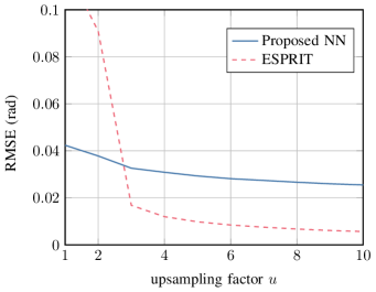
Figure 2: RMSE for present and detected targets with and without cancellation with ESPRIT benchmark SNR of $0\,$dB for the radar channel and $20\,$dB for the communication channel ($M=4$) and $1$ possible target

Comparison of counting encoding and one-hot encoding shows their suitability for the studied problem, yet control of the weighted false alarm rate is much tighter in the counting encoding as shown in Fig. 3. We choose the same training parameters for both simulations, with an evaluation of $20$ batches of $N=10^{4}$ values for each training epoch. During training, the weighted false alarm rate of the counting encoding never exceeds the targeted value $P_{\text{f}}$ by more than $10\%$. Meanwhile, the one-hot encoding oscillates around a weighted false alarm rate of $P_{\text{f}}\approx 3\cdot 10^{-2}$. For applications that generally need to ensure that a given weighted false alarm rate is kept, the counting encoding is more promising. Additionally, counting encoding has computational advantages: The target detection NN output layer saves one neuron and the estimated angle vector can be directly element-wise multiplied with the decision output to calculate one angle estimate for each detected target.

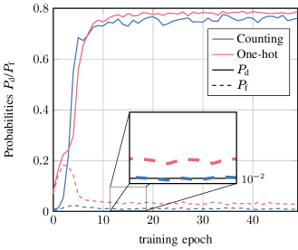
Figure 3: Comparison of detection and weighted false alarm rate of one-hot and counting encoding for an SNR of $0\,$dB for the radar channel and $20\,$dB for the communication channel ($M=4$) for $1$ radar target

III-C Multiple Target Results

Next, we consider the detection of multiple targets with $T_{\max}=3$ while keeping the communication SNR and radar SNR both at $20\,$dB. We trained the system with a total of $9\cdot 10^{7}$ samples. Training angle estimation and target detection sequentially followed by joint training decreased the angle RMSE from roughly $0.1$ to $0.04$. By repeating each training epoch for $1$ to $T_{\max}$ targets, the detection rate for one snapshot rose from approximately $0.6$ to $0.8$. For the radar path, the introduction of multiple targets means that we now observe multiple reflections, leading to an increased signal-to-noise-and-interference ratio (SINR). Comparison of the results of the two encoding metrics shows again how the counting encoding stabilizes the weighted false alarm rate around $P_{\text{f}}\approx 0.01$, while the one-hot encoding settles at $P_{\text{f}}\approx 0.0002$. This causes a much lower detection rate of approximately $0.5$. We also reach a higher RMSE of $0.06$ for the estimated angles.

In Fig. 4, we plot the RMSE of the angle estimation for detected and present targets for $10^{5}$ transmissions versus the upsampling factor $u$. We compare the different set methods from Sec. II-F and also show the ESPRIT benchmark. For the multiple target case, the different set methods enable training of the NNs. The method labeled “None” denotes NN training without using any set method and shows that the implementation of a set method for multiple target estimation is necessary. The permute method performs the best, which was expected since it considers all possible set permutations while still using the MSE loss. The methods based on sorting perform relatively well and are only slightly outperformed by permuting. These set methods outperform the ESPRIT benchmark for small upsampling factors $u\leq 3$. The specific single-snapshot ESPRIT implementation as used for $u=1$ cannot outperform the proposed system.

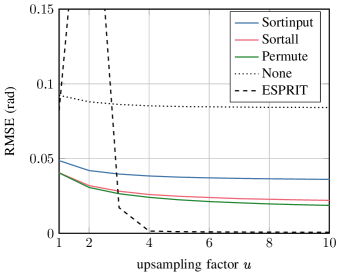
Figure 4: RMSE for present targets with ESPRIT benchmark SNR of $\sigma_{\text{r}}^{2}/\sigma_{\text{n}}^{2}=\nobreak 20\,$dB for the radar channel and $20\,$dB for the communication channel ($M=\nobreak 8$, $T_{\max}=3$)

The detection probability is comparable for all set methods. The weighted false alarm rates are also similar for all methods and converge from the targeted $P_{\text{f}}$ to zero with an increasing $u$. The detection rate saturates to a value of $0.83$ while increasing $u$. For increased detection rate for rising $u$, the detection threshold needs to be further modified.

IV Conclusion

In this work, we demonstrate the feasibility of the AE approach to JCAS for multiple targets. We evaluated different set methods that enable training of angle estimation for multiple targets. Depending on the permissible system complexity, all three options remain contenders for application in future systems. We outperformed an ESPRIT benchmark for angle estimation for small upsampling factors $u$. The novel counting encoding enables setting a design false alarm rate that constraints the detection rate of a NN target detector. We see counting encoding as a promising alternative to classification using one-hot encoding for problems that include object recognition connected with counting. The proposed method is particularly suitable for JCAS systems, where the number of available snapshots is typically limited.

References

- [1] T. Wild, V. Braun, and H. Viswanathan, “Joint design of communication and sensing for beyond 5G and 6G systems,” IEEE Access, vol. 9, 2021.
- [2] F. Lampel, R. F. Tigrek, A. Alvarado, and F. M. Willems, “A performance enhancement technique for a joint FMCW radcom system,” in Proc. Eur. Radar Conf. (EuRAD), 2019.
- [3] C. Sturm and W. Wiesbeck, “Waveform design and signal processing aspects for fusion of wireless communications and radar sensing,” Proc. IEEE, vol. 99, no. 7, 2011.
- [4] M. Braun, C. Sturm, and F. K. Jondral, “Maximum likelihood speed and distance estimation for OFDM radar,” in Proc. IEEE Radar Conf., 2010.
- [5] J. M. Mateos-Ramos, J. Song, Y. Wu, C. Häger, M. F. Keskin, V. Yajnanarayana, and H. Wymeersch, “End-to-end learning for integrated sensing and communication,” in Proc. IEEE Int. Conf. Commun. (ICC), 2022.
- [6] T. O'Shea and J. Hoydis, “An introduction to deep learning for the physical layer,” IEEE Trans. Cogn. Commun. Netw., vol. 3, no. 4, 2017.
- [7] S. Cammerer, F. Ait Aoudia, S. Dörner, M. Stark, J. Hoydis, and S. ten Brink, “Trainable communication systems: concepts and prototype,” IEEE Trans. Commun., vol. 68, no. 9, 2020.
- [8] M. P. Jarabo-Amores, R. Gil-Pita, M. Rosa-Zurera, F. López-Ferreras, and R. Vicen-Bueno, “MLP-based radar detectors for Swerling 1 targets,” Proc. Pattern Recognit. Image Analysis, vol. 18, no. 1, 2008.
- [9] J. Fuchs, A. Dubey, M. Lubke, R. Weigel, and F. Lurz, “Automotive radar interference mitigation using a convolutional autoencoder,” in Proc. IEEE Int. Radar Conf. (RADAR), 2020.
- [10] H. L. van Trees, Optimum Array Processing: Part IV of Detection, Estimation, and Modulation Theory. Wiley, 2002.
- [11] N. Yilmazer, T. K. Sarkar, and M. Salazar-Palma, “DOA estimation using matrix pencil and ESPRIT methods using single and multiple snapshots,” in Proc. URSI EMTS, 2010.
- [12] W. Li, W. Liao, and A. Fannjiang, “Super-resolution limit of the ESPRIT algorithm,” IEEE Trans. Inf. Theory, vol. 66, no. 7, 2020.