RainDiffusion: When Unsupervised Learning Meets Diffusion Models for Real-world Image Deraining

Abstract

Recent diffusion models show great potential in generative modeling tasks. This motivates us to raise an intriguing question – What will happen when unsupervised learning meets diffusion models for real-world image deraining? Before answering it, we observe two major obstacles of diffusion models in real-world image deraining: the need for paired training data and the limited utilization of multi-scale rain patterns. To overcome the obstacles, we propose RainDiffusion, the first real-world image deraining paradigm based on diffusion models. RainDiffusion is a non-adversarial training paradigm that introduces stable training of unpaired real-world data, rather than weakly adversarial training, serving as a new standard bar for real-world image deraining. It consists of two cooperative branches: Non-diffusive Translation Branch (NTB) and Diffusive Translation Branch (DTB). NTB exploits a cycle-consistent architecture to bypass the difficulty in unpaired training of regular diffusion models by generating initial clean/rainy image pairs. Given initial image pairs, DTB leverages multi-scale diffusion models to progressively refine the desired output via diffusive generative and multi-scale priors, to obtain a better generalization capacity of real-world image deraining. Extensive experiments confirm the superiority of our RainDiffusion over eight un/semi-supervised methods and show its competitive advantages over seven fully-supervised ones.

(a) Real rainy image

(b) MSPFN[19]

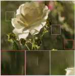
(c) Syn2Real[47]

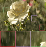
(d) CycleGAN[53]

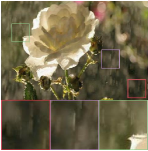
(e) NLCL[49]

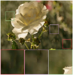
(f) Ours

Figure 1: Image deraining results on a real-world rainy image. From (a) to (f): (a) the real rainy image, and the supervised learning results of (b) MSPFN; the semi-supervised learning results of (c) Syn2Real; the unsupervised results of (d) CycleGAN, (e) NLCL and (f) our RainDiffusion, respectively. RainDiffusion generates both rain-free and perceptually more pleasing results.

1 Introduction

Images captured under complicated rainy scenarios inevitably suffer from the noticeable degradation of visual quality. This degradation causes detrimental impacts on many vision tasks, including segmentation [26], object detection [45], and video surveillance [37]. Thus, it is indispensable to develop effective algorithms to recover quality rain-free images, which is referred to as image deraining.

Image deraining is an ill-posed problem. To make it well-posed, traditional methods typically utilize diverse image priors, such as sparse coding [27], Gaussian Mixture Model [25], and low-rank representation [2]. However, these hand-crafted priors exhibit a limited representation capacity, leading to poor deraining results under complicated and varied rainy scenarios. By learning from massive synthetic clean/rainy image pairs, the performance of deep learning based techniques is substantially improved [46, 12]. Despite their successes, these supervised methods usually achieve sub-optimal performance on real-world rainy images, because of i) the existence of the domain gap between synthetic and real-world rainy images, and ii) the difficulty to collect large-scale real-world clean/rainy image pairs.

To alleviate the aforementioned problems, semi-supervised deraining techniques, as promising solutions, leverage paired synthetic data for good initialization and unpaired real-world data for generalization [41, 48, 47]. But the transferability is still limited since the rain patterns of synthetic images are fixed while the rain patterns of real-world images are dynamically changing. Furthermore, The introduction of CycleGAN [53] makes Generative Adversarial Networks (GANs) the preferred model family for real-world image deraining tasks, as they avoid the need for paired data [43, 16, 20, 52, 4]. However, these GAN-based methods are known as being difficult to train due to their complex adversarial objectives. As a result, they are susceptible to a series of problems, such as premature convergence, model collapse, and optimization instability, leading to image degradation including the loss of image details, remnant rain, halo artifacts, and/or color distortion. More recently, diffusion models [34, 18, 36] have garnered significant attention for their effectiveness in a wide range of generative modeling tasks, such as image inpainting [28], image restoration [29], and image super-resolution [32].

Compared to GANs, diffusion models offer a stable training process and exhibit greater efficacy in modeling the pixel distribution of images. However, no work to-date explores what will happen when unsupervised learning meets diffusion models for real-world image deraining. We have identified two major obstacles to their practical application in real-world image deraining:

• Real-world rainy images lack corresponding clean images, which poses a challenge for existing diffusion models that typically prioritize synthetic degradation scenarios, where generating large-scale paired synthetic data is easier than for real-world examples. Models trained on paired synthetic data struggle to effectively handle complex real-world rain.

• Real-world rainy images comprise diverse rain patterns across different scales, including varying directions, densities, sizes, etc. These multi-scale rain patterns exhibit obvious self-similarity, implying that correlated messages across different scales can potentially enhance the feature representation capability. However, existing diffusion models are primarily designed for single-scale image processing.

In this paper, we propose a novel unsupervised learning paradigm based on diffusion models, called RainDiffusion, to tackle the unfavorable prevailing problem of real-world image deraining. To overcome the two major obstacles identified in applying diffusion models to real-world image deraining, RainDiffusion includes two main interactive branches: Non-diffusive Translation Branch (NTB) and Diffusive Translation Branch (DTB). To bypass the difficulty in unpaired training of regular diffusion models, NTB, only used in the model training phase, makes the best use of cycle-consistent architectures to generate initial clean/rainy image pairs for diffusion model training. Given initial image pairs, DTB employs multi-scale diffusion models that integrate both diffusion generative and multi-scale priors to achieve high-quality real-world image deraining. Instead of using popular unsupervised adversarial networks, RainDiffusion takes advantage of the powerful generative ability of diffusion models to mitigate the limitation of unstable training and produce high-quality derained images (see Fig. 1).

Experiments on five benchmark datasets show that RainDiffusion outperforms existing un/semi-supervised methods and achieves comparable performance against fully-supervised ones. The main contributions are as follows:

• Stable Non-GAN-based Unsupervised Training Paradigm for Real-world Image Deraining. We propose a novel unsupervised image deraining method based on diffusion models, called RainDiffusion. It is a non-adversarial training paradigm, serving as a new standard bar for real-world image deraining.

• First Multi-scale Diffusion-based Model for Unpaired Real-world Data. RainDiffusion consists of two main interactive branches: Non-diffusive Translation Branch (NTB) and Diffusive Translation Branch (DTB). Through these two branches, RainDiffusion is capable of removing the dependency on paired training data and learning the correlation of multi-scale rain streaks for high-quality image deraining.

• State-of-the-art Image Deraining Performance. Extensive experiments show the superiority of RainDiffusion in real-world image deraining. Moreover, our approach performs favorably against existing semi-supervised, unsupervised, and even supervised methods on synthetic datasets.

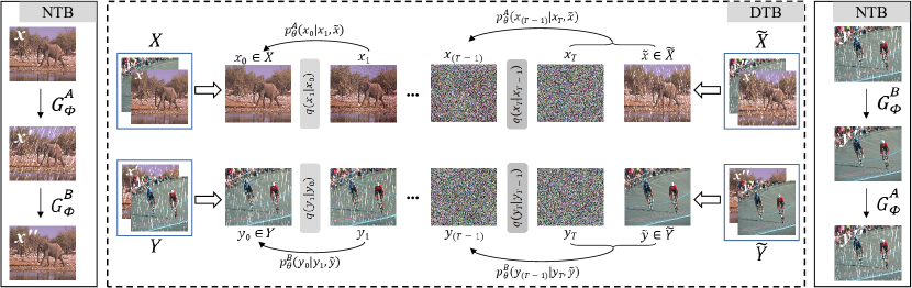
Figure 2: The pipeline of RainDiffusion. It consists of two main interactive branches: Non-diffusive Translation Branch (NTB) and Diffusive Translation Branch (DTB). NTB, only used in the model training phase, fully exploits a cycle-consistent architecture to generate initial clean/rainy image pairs. Note that $G_{\phi}^{A}$ and $G_{\phi}^{B}$ are employed to produce the rainy and rain-free images, respectively. $x$, $y$, $x^{\prime}$, $y^{\prime}$, $x^{\prime\prime}$ and $y^{\prime\prime}$ refer to the given rain-free image, given rainy image, generated rainy image, generated rain-free image, reconstructed rain-free image, and reconstructed rainy image, respectively. Given initial image pairs, DTB leverages two multi-scale diffusion models for translation between clean and rainy images. Especially, the deraining diffusion model learns a conditional reverse process $p_{\theta}^{A}(x_{0:T}|\tilde{x})$ without modifying the diffusion process $q(x_{1:T}|x_{0})$ for $x$. The rain generation diffusion model is similar to it, except it works oppositely.

2 Related Work

Single Image Deraining. Early single image deraining methods employ several hand-crafted priors to restore the rainy images. For example, in [27, 21], it is assumed that rain streaks in the image are both sparse and of high frequency, and thus the problem is translated into a progressive image decomposition process through dictionary learning. Li et al. [25] employ the Gaussian Mixture Model (GMM) to accommodate the presence of multiple orientations and scales of rain streaks. In [5, 2], the low-rank representations are incorporated into deraining. In [15] and [40], guided filter and analysis sparse representation are integrated into sparse coding to achieve finer layer decomposition.

Recently, deep learning based methods have been substantiated to be effective in image deraining [8]. The pioneering work [8] introduces an end-to-end residual convolutional neural network (CNN) for simplifying the learning process. Network modules, such as dense block [23, 38], recursive block [7, 24] and dilated convolution [6], and structures, such as RNN [24, 30], GAN [51, 4] and multi-stream networks [46, 50], are validated to be effective in image deraining. Despite the promising deraining results on synthetic datasets, the learning based methods trained on such synthetic images generalize poorly to real-world images, typically because of the obvious domain gap.

To bridge the domain gap between synthetic and real-world rainy images, several semi-supervised frameworks have been proposed [41, 48, 47]. For example, Wei et al. [41] propose a semi-supervised framework for rain removal, in which they employ a Gaussian Mixture Model (GMM) with a likelihood term and minimize the Kullback-Leibler (KL) divergence between synthetic and real rain. Yasarla et al. [47] further propose a Gaussian Process-based semi-supervised learning framework to achieve improved generalization performance. However, these supervised/semi-supervised methods still require paired data, which is challenging or even impossible to obtain in real-world rainy scenes. Motivated by the success of CycleGAN [53], a popular image-to-image translation architecture, recent works [52, 20, 42, 4] attempt to exploit the improved CycleGAN architecture and constrained transfer learning to jointly learn the rainy and rain-free image domains. However, these GAN-based methods heavily rely on complex adversarial objectives to develop their algorithms, which makes it difficult to achieve stable training. Hence, they also struggle to deliver promising results in real-world image deraining.

Denoising Diffusion Probabilistic Models. Recently, denoising diffusion probabilistic models (DDPM) [34, 18, 36] have exhibited their powerful ability in many vision tasks, such as image super-resolution [32], text-to-image generation [14], and image segmentation [1]. More recently, Özdenizci et al. [29] propose patch-based denoising diffusion models to demonstrate how diffusion models can be used for image restoration. However, these architectures have not been applied to real-world image deraining. They still require paired data for training and ignore multi-scale effects in rain modeling. This observation serves as a motivation for us to propose the first diffusion-based model for real-world image deraining.

3 Proposed Method

The overall architecture of RainDiffusion is presented in Fig. 2. To the best of our knowledge, RainDiffusion is the first diffusion-based model for real-world image deraining. It consists of two main interactive branches: Non-diffusive Translation Branch (NTB) and Diffusive Translation Branch (DTB). The NTB guides the generation of initial clean/rainy image pairs, while the DTB utilizes two multi-scale diffusion models to constrain the translation between clean and rainy images. In the following, we will provide a brief introduction to the diffusion models, followed by a detailed explanation of the NTB and DTB.

3.1 Denoising Diffusion Probabilistic Models

Denoising diffusion probabilistic models (DDPM) slowly corrupt the training data with Gaussian noise and learn to reverse this corruption as a generative model [34, 18, 36]. In the forward process, Gaussian noise is added sequentially onto an input image $x_{0}\sim q(x_{0})$ over $T$ time steps according to the following Markovian process:

$$q(x_{t}|x_{t-1})=\mathcal{N}(x_{t};\sqrt{1-\beta_{t}}x_{t-1},\beta_{t}I),\forall t\in\{1,...,T\}$$ (1)

$$q(x_{1:T}|x_{0})=\prod_{t=1}^{T}q(x_{t}|x_{t-1})$$ (2)

where $\beta_{t}$ is noise variance, $\mathcal{N}(.)$ is a Gaussian distribution, $I$ is an identity covariance matrix with the same dimensions as the input image $x_{0}$. An important property of this recursive formulation is its ability to directly sample $x_{t}$ when $t$ is uniformly drawn from a distribution, i.e., $\forall t\sim\mathcal{U}(\{1,...,T\})$:

$$q(x_{t}|x_{0}) =\mathcal{N}(x_{t};\sqrt{\overline{\alpha}_{t}}x_{0},(1-\overline{\alpha}_{t})I)\Longrightarrow$$ (3)

$$x_{t} =\sqrt{\overline{\alpha}_{t}}x_{0}+\epsilon_{t}\sqrt{1-\overline{\alpha}_{t}}$$

where $\epsilon_{t}\sim\mathcal{N}(0,I)$, $\alpha_{t}=1-\beta_{t}$ and $\overline{\alpha}_{t}=\prod_{i=1}^{t}\alpha_{i}$. Given the original image $x_{0}$ and a fixed variance schedule $\beta_{t}$, we can generate any noisy version $x_{t}$ through a single step of sampling. Similarly, reverse diffusion also adopts a Markov chain from $x_{T}$ onto $x_{0}$, albeit each step aims to gradually denoise the samples. Even though the reverse transition probability between $x_{t}$ and $x_{t-1}$ can be approximated as a Gaussian distribution under small $\beta_{t}$ and large $T$:

$$p_{\theta}(x_{t-1}|x_{t})=\mathcal{N}(x_{t-1};\mu_{\theta}(x_{t},t),\sigma_{\theta}(x_{t},t))$$ (4)

$$p_{\theta}(x_{0:T})=p(x_{T})\prod_{t=1}^{T}p_{\theta}(x_{t-1}|x_{t})$$ (5)

where the reverse process is parameterized by a neural network to estimate $\mu_{\theta}(x_{t},t)$ and $\sigma_{\theta}(x_{t},t)$. $\beta_{t}$ can either be learned in conjunction with the model or kept constant to ensure that $x_{t}$ approximates a standard normal distribution.

The model then can be trained by optimizing a variational bound on negative data log likelihood $\mathbb{E}_{q(x_{0})}[-\log p_{\theta}(x_{0})]\leq L_{\theta}$, which can be performed by:

$$L_{\theta}=\mathbb{E}_{q}[\underbrace{D_{KL}(q(x_{T}|x_{0})||p(x_{T}))}_{L_{T}}\underbrace{-\log p_{\theta}(x_{0}|x_{1})}_{L_{0}}$$ (6)

$$+\sum_{t>1}\underbrace{D_{KL}(q(x_{t-1}|x_{t}),x_{0})||p_{\theta}(x_{t-1}|x_{t}))}_{L_{t-1}}]$$

where $D_{KL}$ refers to the Kullback-Leibler divergence between two probability distributions. A common parametrization focuses on $\mu_{\theta}(x_{t},t)$ while ignoring $\sigma_{\theta}(x_{t},t)$ [18] as follows:

$$\mu_{\theta}(x_{t},t)=\frac{1}{\sqrt{\alpha_{t}}}(x_{t}-\frac{\beta_{t}}{\sqrt{1-\overline{\alpha}_{t}}}\epsilon_{\theta}(x_{t},t))$$ (7)

In this case, the network can be used to estimate the added noise $\epsilon_{t}$ by minimizing the following loss:

$$L_{err}=\mathbb{E}_{x_{0},t,\epsilon_{t}\sim\mathcal{N}(0,I)}[||\epsilon_{t}-\epsilon_{\theta}(\sqrt{\overline{\alpha}_{t}}x_{0}+\epsilon_{t}\sqrt{1-\overline{\alpha}_{t}},t)||^{2}]$$ (8)

During inference, reverse diffusion steps are performed starting from a random sample $x_{T}\sim\mathcal{N}(0,I)$. For each step $t\in\{T,...,1\}$, $\mu$ is derived by Eq. 7 based on the estimated $\epsilon_{\theta}$, and $x_{t-1}$ is sampled based on Eq. 4 as:

$$x_{t-1}=\frac{1}{\sqrt{\alpha_{t}}}(x_{t}-\frac{\beta_{t}}{\sqrt{1-\overline{\alpha}_{t}}}\epsilon_{\theta}(x_{t},t))+\sigma_{t}z$$ (9)

where $z\sim\mathcal{N}(0,I)$), which resembles one step of sampling via Langevin dynamics [44].

To achieve high-quality image deraining, we need to learn a conditional reverse process $p_{\theta}(x_{0:T}|\tilde{x})$ without modifying the diffusion process $q(x_{1:T}|x_{0})$ for $x$, where $x_{0}$ and $\tilde{x}$ represent a clean image and a rainy image, respectively. During the training phase, we sample $(x_{0},\tilde{x})\sim q(x_{0},\tilde{x})$ from a paired data distribution and learn a conditional diffusion model. We input $\tilde{x}$ to the reverse process as:

$$p_{\theta}(x_{0:T}|\tilde{x})=p(x_{T})\prod_{t=1}^{T}p_{\theta}(x_{t-1}|x_{t},\tilde{x})$$ (10)

The noise estimators in Eqs. 7-9 are also replaced by $\epsilon_{\theta}(x_{t},\tilde{x},t)$.

3.2 Non-diffusive Translation Branch (NTB)

Despite the impressive performance of diffusion models in image-conditional data synthesis and restoration [29, 32], their implementation still demands paired clean/rainy images. We will tackle this problem by designing a new Non-diffusive Translation Branch (NTB) without requiring adversarial training. As shown in Fig. 2, NTB incorporates two cycle-consistent circuits to produce an initial set of clean/rainy image pairs for the diffusion model training: 1) rain-free to rain-free translation $x\Rightarrow x^{\prime}\Rightarrow x^{\prime\prime}$; 2) rainy to rainy translation $y\Rightarrow y^{\prime}\Rightarrow y^{\prime\prime}$.

Given unpaired rainy image $y$ and clean image $x$, NTB employs two non-diffusive generators with parameters $\phi^{A,B}$ to obtain initial translation estimates:

$$\centering\begin{split}x^{\prime}=G_{\phi}^{A}(x)\qquad x^{\prime\prime}=G_{\phi}^{B}(x^{\prime})\\ y^{\prime}=G_{\phi}^{B}(y)\qquad y^{\prime\prime}=G_{\phi}^{A}(y^{\prime})\end{split}\@add@centering$$ (11)

where $x$, $y$, $x^{\prime}$, $y^{\prime}$, $x^{\prime\prime}$ and $y^{\prime\prime}$ refer to the given rain-free image, given rainy image, generated rainy image, generated rain-free image, reconstructed rain-free image, and reconstructed rainy image, respectively. We adopt U-Net [31] as our non-diffusive generators. The cycle-consistency loss is employed to confine the generated samples within a limited space and preserve the contents of the generated images:

$$L_{cyc}=E_{x\sim P_{data(x)}}[\left\|x^{\prime\prime}-x\right\|_{1}]+E_{y\sim P_{data(y)}}[\left\|y^{\prime\prime}-y\right\|_{1}]$$ (12)

The difference between NTB and other circulatory structures. In unsupervised learning, the circulatory structures with cycle-consistency loss are commonly used for model training [4, 42, 53]. The differences between NTB and others lie in two aspects: 1) NTB requires no discriminators for adversarial training. This means that NTB provides a reliable non-adversarial training process. 2) The generators of NTB are designed to generate paired clean/rainy images for diffusion model training. Thus, both $G_{\phi}^{A}$ and $G_{\phi}^{B}$ are only used in the training phase and remain uninvolved in the testing phase for image deraining.

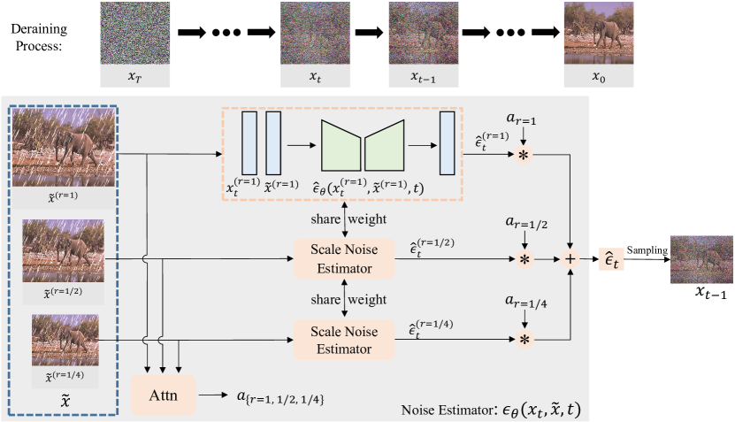
Figure 3: The pipeline of multi-scale diffusion model.

Algorithm 1 The training of RainDiffusion

0:  Unpaired clean image $x$ and rainy image $y$

1:  repeat

2:     $x^{\prime}=G_{\phi}^{A}(x),x^{\prime\prime}=G_{\phi}^{B}(x^{\prime})$

3:     $y^{\prime}=G_{\phi}^{B}(y),y^{\prime\prime}=G_{\phi}^{A}(y^{\prime})$

4:     $t^{A},t^{B}\sim$ Uniform $(\{1,...,T\})$

5:     $\epsilon^{A},\epsilon^{B}\sim\mathcal{N}(0,I)$

6:     Take gradient descent step on

7:     $\nabla_{\theta,\phi}[||\epsilon^{A}-\epsilon_{\theta}^{A}(\sqrt{\overline{\alpha}_{t^{A}}}x+\epsilon_{t^{A}}\sqrt{1-{\overline{\alpha}_{t^{A}}}},x^{\prime},t^{A})||^{2}$

8:     $+||\epsilon^{B}-\epsilon_{\theta}^{B}(\sqrt{\overline{\alpha}_{t^{B}}}x^{\prime}+\epsilon_{t^{B}}\sqrt{1-{\overline{\alpha}_{t^{B}}}},x^{\prime\prime},t^{B})||^{2}$

9:     $+||\epsilon^{B}-\epsilon_{\theta}^{B}(\sqrt{\overline{\alpha}_{t^{B}}}y+\epsilon_{t^{B}}\sqrt{1-{\overline{\alpha}_{t^{B}}}},y^{\prime},t^{B})||^{2}$

10:     $+||\epsilon^{A}-\epsilon_{\theta}^{A}(\sqrt{\overline{\alpha}_{t^{A}}}y^{\prime}+\epsilon_{t^{A}}\sqrt{1-{\overline{\alpha}_{t^{A}}}},y^{\prime\prime},t^{A})||^{2}$

11:     $+\lambda_{cyc}L_{cyc}]$

12:  until converged

13:  return $\theta^{A}$(deraining), $\theta^{B}$(rain generation)

3.3 Diffusive Translation Branch (DTB)

Following the advantage of diffusion models in the area of generative modeling, DTB utilizes diffusion models to mitigate the limitation of unstable training and improve the generalization ability for image deraining. Like NTB, DTB also employs a pair of diffusion models for image deraining and rain generation, respectively, as illustrated in Fig. 2. The deraining diffusion model learns a conditional reverse process $p_{\theta}^{A}(x_{0:T}|\tilde{x})$ without modifying the diffusion process $q(x_{1:T}|x_{0})$ for $x$.

In real-world scenes, rain artifacts exhibit diverseness, but not limited to varying directions, densities, and sizes. This presents a considerable challenge in directly implementing diffusion models to perform real-world image deraining. We notice that the rain streak patterns change relatively little across different scales. Thus, we incorporate this correlation of rain streaks across different scales into the diffusion generative process. Beyond existing fixed-scale diffusion models [29, 32], we design multi-scale diffusion models for image deraining (see Fig. 3).

At each time step $t$, when provided with an intermediate sample $x_{t}$ and a rainy image $\tilde{x}$, our initial step involves downsampling the original images into various scales, such as 1/2 and 1/4, as represented by:

$$\{x_{t}^{r},\tilde{x}^{r}\}=down(x_{t},\tilde{x}),r\in\{1,1/2,1/4\}$$ (13)

where $r$ represents the scale of the image. To make full use of multi-scale information for deraining, we then use attention heads [3] to learn all attention masks $\alpha_{r=\{1,1/2,1/4\}}$ for each of a fixed set of scales, which can be used to weight the multi-scale features at each pixel location. For each scale branch, the scale noise estimator $\hat{\epsilon}_{\theta}$ receives the intermediate variable $x_{t}^{r}$ and rainy image $\tilde{x}^{r}$ from a single (lower) scale $r$ along with the time step $t$ as input, to predict the noise map $\hat{\epsilon}^{r}_{t}$ from the scale $r$ as:

$$\hat{\epsilon}^{r}_{t}=\hat{\epsilon}_{\theta}(x_{t}^{r},\tilde{x}^{r},t)$$ (14)

similar to most of existing diffusion models, we employ U-Net [31] as the scale noise estimator. We combine the noise maps from multiple scales, i.e., $\hat{\epsilon}^{r\in\{1,1/2,1/4\}}_{t}$, by multiplying the attention masks $\alpha_{r=\{1,1/2,1/4\}}$ with the maps in a pixel-wise manner, and then summing the results across different scales to obtain the final noise map $\hat{\epsilon}_{t}$. The whole noise estimator $\epsilon_{\theta}(x_{t},\tilde{x},t)$ is expressed as:

$$\epsilon_{\theta}(x_{t},\tilde{x},t)=\hat{\epsilon}_{t}=\sum^{N}_{i=1}a_{r}\ast\hat{\epsilon}^{r}_{t}$$ (15)

where $N$ denotes the total number of different scales $r$. The training phase of RainDiffusion is outlined in Algorithm 1.

Algorithm 2 The testing of RainDiffusion

0:  Rainy image $\tilde{x}$, deraining noise estimator $\epsilon_{\theta}^{A}(x_{t},\tilde{x},t)$, number of implicit sampling iterations $T$.

1:  $x_{t}\sim\mathcal{N}(0,I)$

2:  for each $i=S,...,1$ do

3:     $t=(i-1)\cdot T/S+1$

4:     $t_{next}=(i-2)\cdot T/S+1$ if $i>1$ else 0

5:     $\hat{\epsilon}_{t}^{A}=\epsilon_{\theta}^{A}(x_{t},\tilde{x},t)$

6:     $x_{t-1}=\sqrt{\overline{\alpha}_{t_{next}}}(\frac{x_{t}-\sqrt{1-\overline{\alpha}_{t}}\cdot\hat{\epsilon}_{t}^{A}}{\sqrt{\overline{\alpha}_{t}}})+\sqrt{1-\overline{\alpha}_{t_{next}}}\cdot\hat{\epsilon}_{t}^{A}$

7:  end for

8:  return $x_{0}$

The testing phase of RainDiffusion is outlined in Algorithm 2. We observe that a large $T$ inevitably leads to costly sampling, e.g., when $T=1000$. To address this problem, we use an implicit sampling strategy [35] to accelerate our sampling process (lines 3-4 in Alg. 2). Implicit sampling with a noise estimator $\epsilon_{\theta}(x_{t},\tilde{x},t)$ can be performed by

$$\begin{split}x_{t-1}=&\sqrt{\overline{\alpha}_{t-1}}(\frac{x_{t}-\sqrt{1-\overline{\alpha}_{t}}\cdot\epsilon_{\theta}(x_{t},\tilde{x},t)}{\sqrt{\overline{\alpha}_{t}}})\\ &+\sqrt{1-\overline{\alpha}_{t-1}}\cdot\epsilon_{\theta}(x_{t},\tilde{x},t)\end{split}$$ (16)

during accelerated sampling we only needs a subsequence $\tau_{1},...,\tau_{S}$ of the complete ${1,...,T}$ timestep indices, which can be performed by

$$\begin{split}\tau_{i}=(i-1)\cdot T/S+1\end{split}$$ (17)

At any denoising time step $t$, according to Eq. 15, we utilize the deraining noise estimator $\epsilon_{\theta}^{A}(x_{t},\tilde{x},t)$ from line 13 in Alg. 1 to estimate the noise map $\hat{\epsilon}^{A}_{t}$ (line 5 in Alg. 2). Subsequently, we perform an implicit sampling update utilizing the noise map $\hat{\epsilon}^{A}_{t}$ (line 6 in Alg. 2).

The proposed DTB constructs the multi-scale diffusion models, which incorporate multi-scale rain information into the diffusion generative process and introduce an attention mechanism that softly weights the multi-scale features at each pixel location. Thereby, they are more compact and robust than several existing multi-scale fusion approaches [19, 11]. Notably, we use the same diffusion process configuration for rain generation, except it works oppositely.

Table 1: Descriptions of different benchmark training datasets.

Datasets	Rain200H	Rain200L	Rain800	DDN-Data	SPA-Data
Train-Set	1800	1800	700	12600	28500
Test-Set	200	200	100	1400	1000
Type	Synthetic				Real-world

Table 2: Comparisons of different deraining methods. Red and blue colors indicate the $1^{st}$ and $2^{nd}$ ranks, respectively.

Datasets		Rain200H		Rain200L		Rain800		DDN-Data		SPA-Data
Metrics		PSNR	SSIM	PSNR	SSIM	PSNR	SSIM	PSNR	SSIM	PSNR	SSIM
Prior-based	DSC [27]	13.17	0.427	27.34	0.849	18.56	0.600	27.31	0.837	34.95	0.942
	GMM [25]	13.04	0.467	29.05	0.872	20.46	0.730	26.87	0.808	34.30	0.943
Supervised	DDN [10]	24.64	0.849	34.68	0.967	21.16	0.732	28.00	0.873	34.70	0.934
	DID-MDN [50]	25.61	0.854	35.40	0.961	21.89	0.795	26.38	0.835	34.68	0.930
	SPA-Net [39]	26.07	0.857	31.59	0.919	24.37	0.861	29.83	0.904	35.13	0.944
	MSPFN [19]	28.66	0.870	32.40	0.933	26.91	0.882	32.93	0.923	34.87	0.952
	AirNet [22]	25.48	0.829	34.90	0.969	23.77	0.833	31.06	0.910	33.45	0.924
Semi-supervised	SIRR [41]	26.55	0.846	34.47	0.969	24.36	0.859	30.01	0.907	34.85	0.936
	Syn2Real [47]	25.76	0.837	34.39	0.965	23.74	0.799	29.29	0.905	33.77	0.953
	JRGR [48]	24.62	0.849	34.51	0.967	24.62	0.828	28.92	0.890	34.12	0.943
Unsupervised	CycleGAN [53]	20.59	0.704	24.61	0.834	23.95	0.819	24.34	0.776	22.40	0.860
	RR-GAN [52]	/	/	/	/	23.51	0.757	/	/	/	/
	DerainCycleGAN [42]	/	/	31.49	0.936	24.32	0.842	/	/	34.12	0.950
	DCD-GAN [4]	/	/	/	/	25.61	0.813	31.65	0.918	35.30	0.943
	NLCL [49]	22.31	0.728	31.74	0.935	24.46	0.821	31.26	0.914	34.94	0.945
	Ours	26.02	0.862	36.85	0.972	26.49	0.875	32.04	0.920	35.40	0.954

4 Experiment

4.1 Experimental Settings

Implementation Details. We implement RainDiffusion using Pytorch 1.6 on an Nvidia GeForce RTX 3090 GPU. For optimizing RainDiffusion, we use the Adam optimizer with a min-batch size of 4 to train the paradigm, where the momentum parameters $\beta_{1}$ and $\beta_{2}$ take the values of 0.5 and 0.999, respectively. The initial learning rate is set to $2e^{-5}$. For training, a 128 $\times$128 image patch is randomly cropped from the original image (or its horizontal flipped version). The balance weight $\lambda_{cyc}$ is set to 1.

Comparison Methods. We qualitatively and quantitatively compare our method with seven supervised methods (i.e., DSC [27], GMM [25], DDN [10], DID-MDN [50], SPA-Net [39], MSPFN [19] and AirNet [22]), three semi-supervised methods (i.e., SIRR [41], Syn2Real [47], and JRGR [48]), as well as five unsupervised methods (i.e., CycleGAN [53], RR-GAN [52], DerainCycleGAN [42], DCD-GAN [4] and NLCL [49]).

Datasets. We employ five challenging benchmark datasets including Rain200H [46], Rain200L [46], Rain800 [51], DDN-Data [9] and SPA-Data [39] with diverse rain streaks of varying sizes, densities, and orientations. The detailed descriptions of the used training and testing datasets are presented in Table 1.

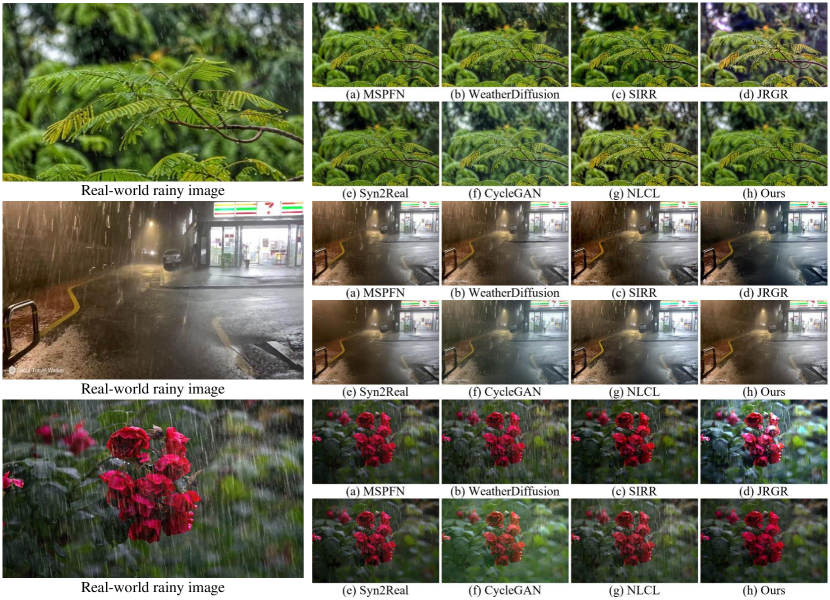
Figure 4: Comparison of deraining performance on real-world rainy images. Most deraining methods fail to remove rain streaks in heavy rain. Comparatively, our method is more successful to remove rain accumulation and obtains the cleanest result with very clear details.

4.2 Comparison with State-of-the-arts

Comparison on Synthetic Datasets. Table 2 presents the quantitative results of different methods on four synthetic datasets. We make the following observations: 1) Compared with unsupervised deraining methods, our method obtains higher values of PSNR and SSIM, which verifies the the excellent performance of the proposed RainDiffusion. 2) There is an obvious performance gap between semi-supervised and supervised methods, which can be even more significant than the gap between RainDiffusion and supervised ones. 3) Our method is capable of achieving competitive results to most of existing supervised ones. More qualitative results on synthetic datasets are provided in the supplementary material.

Comparison on Real-world Datasets. Following the protocol of [4, 13], we further compare RainDiffusion with different methods on the SPA-Data dataset, which comprises real-world rainy images along with their corresponding ground truth for evaluation using the numerical metrics. Table 2 demonstrates that our method achieves superior performance gains to all compared methods, thereby providing compelling evidence for the effectiveness of our approach for real-world image deraining.

Furthermore, we collect 400 unlabeled real-world rainy images from Google image search, which are more complex and challenging than SPA-Data. As shown in Fig. 4, RainDiffusion successfully handles diverse rain streaks with distinct patterns and achieves superior visual results than all compared methods. Notably, the deraining results of unsupervised methods may induce color and structure distortion, whereas our method can better preserve the color and structure of the image. More qualitative results are provided in the supplementary material.

Table 3: Ablation study for different loss functions in Rain800. $L_{err}(\epsilon_{\theta}^{A}(x,x^{\prime}))$ indicates line 7 in Alg. 1.

Model	w/o $L_{err}(\epsilon_{\theta}^{A}(x,x^{\prime}))$	w/o $L_{err}(\epsilon_{\theta}^{B}(x^{\prime},x^{\prime\prime}))$	w/o $L_{cyc}$
PSNR / SSIM	25.02/0.824	25.94/0.862	20.26/0.733
Model	w/o $L_{err}(\epsilon_{\theta}^{B}(y,y^{\prime}))$	w/o $L_{err}(\epsilon_{\theta}^{A}(y^{\prime},y^{\prime\prime}))$	Ours
PSNR / SSIM	25.59/0.851	25.27/0.836	26.49/0.875

Table 4: Ablation study for the variants of our model in Rain800.

Model	SR3	WeatherDiffusion	Ours
PSNR / SSIM	24.45/0.803	25.37/0.839	26.49/0.875
Model	w/o NTB	w/o NTB*	w/o DTB
PSNR / SSIM	25.16/0.835	25.12/0.831	24.65/0.812
Estimator	ResNet-50	VGG-16	U-Net
PSNR / SSIM	24.87/0.821	25.64/0.854	26.49/0.875

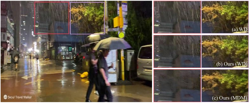
Figure 5: Qualitative analysis of different diffusion models. WD represents WeatherDiffusion [29].

4.3 Ablation Study

The Effect of Loss Function. We evaluate the effectiveness of our hybrid loss function on the Rain800 dataset. Especially, we remove one component to each configuration at one time. For fair comparision, the same training settings are kept for all models testing. As depicted in Table 3, the full structure of RainDiffusion exhibits the highest performance in both PSNR and SSIM metrics, suggesting that all the components of RainDiffusion are advantageous for proficient rain removal. Moreover, we also evaluate the different settings of the balanced weight $\lambda_{cyc}$. The results are provided in the supplementary material.

The Effect of Different Diffusion Models. To validate the effectiveness of the proposed multi-scale diffusion models (MDMs), we choose two recent diffusion-based image restoration methods, i.e., SR3 [32] and WeatherDiffusion [29], as the competing approaches. For fair comparison, we substitute the MDMs in DTB with these two supervised models, and retrain the entire paradigm. Table 4 and Fig. 5 demonstrate that the proposed MDM outperforms the compared methods on both synthetic and real-world rainy images. The obtained results affirm the significance of multi-scale rain information captured by MDM. When incorporating WeatherDiffusion [29] into our unsupervised paradigm, it can achieve satisfactory performance on real-world rainy images without the need for paired data.

The Effect of Additional Translation Procedures. Despite the primary goal of image deraining, there are also several additional translation procedures. To further verify the effect of them, we remove the translations of rain-free to rain-free and rainy to rainy in NTB, and the rain generation diffusion model in DTB as our comparison models, which are denoted as “w/o NTB”, “w/o NTB*”, and “w/o DTB” in Table 4. The result indicates that additional translation procedures can enhance clean exemplars and offer supplementary constraints for improved rain removal.

The Choice of Different Noise Estimators. Apart from U-Net [31], we also adopt other baselines as our scale noise estimators in DTB, such as ResNet-50 [17] and VGG-16 [33]. Table 4 indicates that U-Net is a fitting candidate for the purpose of noise estimation.

Table 5: Ablation study for different scale settings in Rain800.

Settings	V1	V2	V3	V4
$r=1$	✓	✓	✓	✓
$r=1/2$	w/o	✓	w/o	✓
$r=1/4$	w/o	w/o	✓	✓
PSNR	24.96	25.72	25.34	26.49
SSIM	0.822	0.858	0.839	0.875

The Effect of Different Scale Settings. The multi-scale learning strategy provides the capacity of scale-robust rain removal. We perform an ablation analysis of different scale settings as shown in Table 5. It is observed that the combination of scales $r\in\{1,1/2,1/4\}$ yields the best results.

5 Conclusion

In this paper, we avoid any adversarial objectives to bridge the gap between the synthetic and real-world rainy images. We propose a new unsupervised learning paradigm based on diffusion models, called RainDiffusion, to tackle the unfavorable prevailing problem of real-world image deraining. RainDiffusion consists of two main interactive branches: Non-diffusive Translation Branch (NTB) and Diffusive Translation Branch (DTB). Particularly, NTB extensively leverages cycle-consistent architecture to produce preliminary sets of clean/rainy image pairs for diffusion model training. Given initial image pairs, DTB employs multi-scale diffusion models to gradually improve the target output with diffusive generative and multi-scale prior. Experiments on both synthetic and real-world rainy images demonstrate that RainDiffusion performs favorably against current un/semi-supervised methods, and also offers competitive advantages to the fully-supervised ones.

References

- [1] Tomer Amit, Eliya Nachmani, Tal Shaharbany, and Lior Wolf. Segdiff: Image segmentation with diffusion probabilistic models. arXiv preprint arXiv:2112.00390, 2021.
- [2] Yi Chang, Luxin Yan, and Sheng Zhong. Transformed low-rank model for line pattern noise removal. In Proceedings of the IEEE international conference on computer vision, pages 1726–1734, 2017.
- [3] Liang-Chieh Chen, Yi Yang, Jiang Wang, Wei Xu, and Alan L Yuille. Attention to scale: Scale-aware semantic image segmentation. In Proceedings of the IEEE conference on computer vision and pattern recognition, pages 3640–3649, 2016.
- [4] Xiang Chen, Jinshan Pan, Kui Jiang, Yufeng Li, Yufeng Huang, Caihua Kong, Longgang Dai, and Zhentao Fan. Unpaired deep image deraining using dual contrastive learning. In Proceedings of the IEEE/CVF Conference on Computer Vision and Pattern Recognition, pages 2017–2026, 2022.
- [5] Yi-Lei Chen and Chiou-Ting Hsu. A generalized low-rank appearance model for spatio-temporally correlated rain streaks. In Proceedings of the IEEE International Conference on Computer Vision, pages 1968–1975, 2013.
- [6] Sen Deng, Mingqiang Wei, Jun Wang, Yidan Feng, Luming Liang, Haoran Xie, Fu Lee Wang, and Meng Wang. Detail-recovery image deraining via context aggregation networks. In Proceedings of the IEEE/CVF conference on computer vision and pattern recognition, pages 14560–14569, 2020.
- [7] Zhiwen Fan, Huafeng Wu, Xueyang Fu, Yue Huang, and Xinghao Ding. Residual-guide network for single image deraining. In Proceedings of the 26th ACM international conference on Multimedia, pages 1751–1759, 2018.
- [8] Xueyang Fu, Jiabin Huang, Xinghao Ding, Yinghao Liao, and John Paisley. Clearing the skies: A deep network architecture for single-image rain removal. IEEE Transactions on Image Processing, 26(6):2944–2956, 2017.
- [9] Xueyang Fu, Jiabin Huang, Delu Zeng, Yue Huang, Xinghao Ding, and John Paisley. Removing rain from single images via a deep detail network. In Proceedings of the IEEE Conference on Computer Vision and Pattern Recognition, pages 3855–3863, 2017.
- [10] Xueyang Fu, Jiabin Huang, Delu Zeng, Yue Huang, Xinghao Ding, and John W. Paisley. Removing rain from single images via a deep detail network. In 2017 IEEE Conference on Computer Vision and Pattern Recognition, pages 1715–1723, 2017.
- [11] Xueyang Fu, Borong Liang, Yue Huang, Xinghao Ding, and John Paisley. Lightweight pyramid networks for image deraining. IEEE transactions on neural networks and learning systems, 31(6):1794–1807, 2019.
- [12] Xueyang Fu, Qi Qi, Zheng-Jun Zha, Yurui Zhu, and Xinghao Ding. Rain streak removal via dual graph convolutional network. In Proc. AAAI Conf. Artif. Intell., pages 1–9, 2021.
- [13] Xueyang Fu, Jie Xiao, Yurui Zhu, Aiping Liu, Feng Wu, and Zheng-Jun Zha. Continual image deraining with hypergraph convolutional networks. IEEE Transactions on Pattern Analysis and Machine Intelligence, 2023.
- [14] Shuyang Gu, Dong Chen, Jianmin Bao, Fang Wen, Bo Zhang, Dongdong Chen, Lu Yuan, and Baining Guo. Vector quantized diffusion model for text-to-image synthesis. In Proceedings of the IEEE/CVF Conference on Computer Vision and Pattern Recognition, pages 10696–10706, 2022.
- [15] Shuhang Gu, Deyu Meng, Wangmeng Zuo, and Lei Zhang. Joint convolutional analysis and synthesis sparse representation for single image layer separation. In Proceedings of the IEEE International Conference on Computer Vision, pages 1708–1716, 2017.
- [16] Kewen Han and Xinguang Xiang. Decomposed cyclegan for single image deraining with unpaired data. In ICASSP 2020-2020 IEEE International Conference on Acoustics, Speech and Signal Processing (ICASSP), pages 1828–1832. IEEE, 2020.
- [17] Kaiming He, Xiangyu Zhang, Shaoqing Ren, and Jian Sun. Deep residual learning for image recognition. In Proceedings of the IEEE conference on computer vision and pattern recognition, pages 770–778, 2016.
- [18] Jonathan Ho, Ajay Jain, and Pieter Abbeel. Denoising diffusion probabilistic models. Advances in Neural Information Processing Systems, 33:6840–6851, 2020.
- [19] Kui Jiang, Zhongyuan Wang, Peng Yi, Chen Chen, Baojin Huang, Yimin Luo, Jiayi Ma, and Junjun Jiang. Multi-scale progressive fusion network for single image deraining. In Proceedings of the IEEE/CVF conference on computer vision and pattern recognition, pages 8346–8355, 2020.
- [20] Xin Jin, Zhibo Chen, Jianxin Lin, Zhikai Chen, and Wei Zhou. Unsupervised single image deraining with self-supervised constraints. In 2019 IEEE International Conference on Image Processing (ICIP), pages 2761–2765. IEEE, 2019.
- [21] Li-Wei Kang, Chia-Wen Lin, and Yu-Hsiang Fu. Automatic single-image-based rain streaks removal via image decomposition. IEEE transactions on image processing, 21(4):1742–1755, 2011.
- [22] Boyun Li, Xiao Liu, Peng Hu, Zhongqin Wu, Jiancheng Lv, and Xi Peng. All-in-one image restoration for unknown corruption. In Proceedings of the IEEE/CVF Conference on Computer Vision and Pattern Recognition, pages 17452–17462, 2022.
- [23] Guanbin Li, Xiang He, Wei Zhang, Huiyou Chang, Le Dong, and Liang Lin. Non-locally enhanced encoder-decoder network for single image de-raining. In Proceedings of the 26th ACM international conference on Multimedia, pages 1056–1064, 2018.
- [24] Xia Li, Jianlong Wu, Zhouchen Lin, Hong Liu, and Hongbin Zha. Recurrent squeeze-and-excitation context aggregation net for single image deraining. In Proceedings of the European Conference on Computer Vision (ECCV), pages 254–269, 2018.
- [25] Yu Li, Robby T Tan, Xiaojie Guo, Jiangbo Lu, and Michael S Brown. Rain streak removal using layer priors. In Proceedings of the IEEE conference on computer vision and pattern recognition, pages 2736–2744, 2016.
- [26] Li Liu, Wanli Ouyang, Xiaogang Wang, Paul Fieguth, Jie Chen, Xinwang Liu, and Matti Pietikäinen. Deep learning for generic object detection: A survey. International journal of computer vision, 128(2):261–318, 2020.
- [27] Yu Luo, Yong Xu, and Hui Ji. Removing rain from a single image via discriminative sparse coding. In Proceedings of the IEEE international conference on computer vision, pages 3397–3405, 2015.
- [28] Alexander Quinn Nichol, Prafulla Dhariwal, Aditya Ramesh, Pranav Shyam, Pamela Mishkin, Bob Mcgrew, Ilya Sutskever, and Mark Chen. Glide: Towards photorealistic image generation and editing with text-guided diffusion models. In International Conference on Machine Learning, pages 16784–16804. PMLR, 2022.
- [29] Ozan Özdenizci and Robert Legenstein. Restoring vision in adverse weather conditions with patch-based denoising diffusion models. arXiv preprint arXiv:2207.14626, 2022.
- [30] Dongwei Ren, Wangmeng Zuo, Qinghua Hu, Pengfei Zhu, and Deyu Meng. Progressive image deraining networks: a better and simpler baseline. In Proceedings of the IEEE Conference on Computer Vision and Pattern Recognition, pages 3937–3946, 2019.
- [31] Olaf Ronneberger, Philipp Fischer, and Thomas Brox. U-net: Convolutional networks for biomedical image segmentation. In International Conference on Medical image computing and computer-assisted intervention, pages 234–241. Springer, 2015.
- [32] Chitwan Saharia, Jonathan Ho, William Chan, Tim Salimans, David J Fleet, and Mohammad Norouzi. Image super-resolution via iterative refinement. IEEE Transactions on Pattern Analysis and Machine Intelligence, 2022.
- [33] Karen Simonyan and Andrew Zisserman. Very deep convolutional networks for large-scale image recognition. arXiv preprint arXiv:1409.1556, 2014.
- [34] Jascha Sohl-Dickstein, Eric Weiss, Niru Maheswaranathan, and Surya Ganguli. Deep unsupervised learning using nonequilibrium thermodynamics. In International Conference on Machine Learning, pages 2256–2265. PMLR, 2015.
- [35] Jiaming Song, Chenlin Meng, and Stefano Ermon. Denoising diffusion implicit models. arXiv preprint arXiv:2010.02502, 2020.
- [36] Yang Song and Stefano Ermon. Generative modeling by estimating gradients of the data distribution. Advances in Neural Information Processing Systems, 32, 2019.
- [37] Waqas Sultani, Chen Chen, and Mubarak Shah. Real-world anomaly detection in surveillance videos. In Proceedings of the IEEE conference on computer vision and pattern recognition, pages 6479–6488, 2018.
- [38] Guoqing Wang, Changming Sun, and Arcot Sowmya. Erl-net: Entangled representation learning for single image de-raining. In Proceedings of the IEEE International Conference on Computer Vision, pages 5644–5652, 2019.
- [39] Tianyu Wang, Xin Yang, Ke Xu, Shaozhe Chen, Qiang Zhang, and Rynson WH Lau. Spatial attentive single-image deraining with a high quality real rain dataset. In Proceedings of the IEEE Conference on Computer Vision and Pattern Recognition, pages 12270–12279, 2019.
- [40] Yinglong Wang, Shuaicheng Liu, Chen Chen, and Bing Zeng. A hierarchical approach for rain or snow removing in a single color image. IEEE Transactions on Image Processing, 26(8):3936–3950, 2017.
- [41] Wei Wei, Deyu Meng, Qian Zhao, Zongben Xu, and Ying Wu. Semi-supervised transfer learning for image rain removal. In Proceedings of the IEEE Conference on Computer Vision and Pattern Recognition, pages 3877–3886, 2019.
- [42] Yanyan Wei, Zhao Zhang, Yang Wang, Mingliang Xu, Yi Yang, Shuicheng Yan, and Meng Wang. Deraincyclegan: Rain attentive cyclegan for single image deraining and rainmaking. IEEE Transactions on Image Processing, 30:4788–4801, 2021.
- [43] Yanyan Wei, Zhao Zhang, Yang Wang, Haijun Zhang, Mingbo Zhao, Mingliang Xu, and Meng Wang. Semi-deraingan: A new semi-supervised single image deraining. In 2021 IEEE International Conference on Multimedia and Expo (ICME), pages 1–6. IEEE, 2021.
- [44] Max Welling and Yee W Teh. Bayesian learning via stochastic gradient langevin dynamics. In Proceedings of the 28th international conference on machine learning (ICML-11), pages 681–688, 2011.
- [45] Zbigniew Wojna, Vittorio Ferrari, Sergio Guadarrama, Nathan Silberman, Liang-Chieh Chen, Alireza Fathi, and Jasper Uijlings. The devil is in the decoder: Classification, regression and gans. International Journal of Computer Vision, 127(11):1694–1706, 2019.
- [46] Wenhan Yang, Robby T Tan, Jiashi Feng, Jiaying Liu, Zongming Guo, and Shuicheng Yan. Deep joint rain detection and removal from a single image. In Proceedings of the IEEE Conference on Computer Vision and Pattern Recognition, pages 1357–1366, 2017.
- [47] Rajeev Yasarla, Vishwanath A Sindagi, and Vishal M Patel. Syn2real transfer learning for image deraining using gaussian processes. In Proceedings of the IEEE/CVF conference on computer vision and pattern recognition, pages 2726–2736, 2020.
- [48] Yuntong Ye, Yi Chang, Hanyu Zhou, and Luxin Yan. Closing the loop: Joint rain generation and removal via disentangled image translation. In Proceedings of the IEEE/CVF Conference on Computer Vision and Pattern Recognition, pages 2053–2062, 2021.
- [49] Yuntong Ye, Changfeng Yu, Yi Chang, Lin Zhu, Xi-Le Zhao, Luxin Yan, and Yonghong Tian. Unsupervised deraining: Where contrastive learning meets self-similarity. In Proceedings of the IEEE/CVF Conference on Computer Vision and Pattern Recognition, pages 5821–5830, 2022.
- [50] He Zhang and Vishal M Patel. Density-aware single image de-raining using a multi-stream dense network. In Proceedings of the IEEE conference on computer vision and pattern recognition, pages 695–704, 2018.
- [51] He Zhang, Vishwanath Sindagi, and Vishal M Patel. Image de-raining using a conditional generative adversarial network. IEEE transactions on circuits and systems for video technology, 30(11):3943–3956, 2019.
- [52] Hongyuan Zhu, Xi Peng, Joey Tianyi Zhou, Songfan Yang, Vijay Chanderasekh, Liyuan Li, and Joo-Hwee Lim. Singe image rain removal with unpaired information: A differentiable programming perspective. In Proceedings of the AAAI Conference on Artificial Intelligence, volume 33, pages 9332–9339, 2019.
- [53] Jun-Yan Zhu, Taesung Park, Phillip Isola, and Alexei A Efros. Unpaired image-to-image translation using cycle-consistent adversarial networks. In Proceedings of the IEEE international conference on computer vision, pages 2223–2232, 2017.