First measurement of the Q² distribution of X(3915) single-tag two-photon production

Abstract

We report the first measurement of the $Q^{2}$ distribution of $X(3915)$ produced by single-tag two-photon interactions. The decay mode used is $X(3915)\rightarrow J/\psi\omega$. The covered $Q^{2}$ region is from 1.5 (GeV/$c$)² to 10.0 (GeV/$c$)². We observe $7.9\pm 3.1({\rm stat.})\pm 1.5({\rm syst.})$ events, where we expect $4.1\pm 0.7$ events based on the $Q^{2}=0$ result from the no-tag two-photon process, extrapolated to higher $Q^{2}$ region using the $c\bar{c}$ model of Schuler, Berends, and van Gulik. The shape of the distribution is also consistent with this model; we note that statistical uncertainties are large.

I Introduction

The discovery of $X(3872)$ opened a new era of exotic hadrons called charmoniumlike states [1]. Understanding the nature of this state and of other charmoniumlike states, in general, provides an opportunity to study the nonperturbative regime of quantum chromodynamics. In searching for other charmoniumlike states, $X(3915)$ was found by the Belle experiment [2, 3] and confirmed by the BaBar experiment [4, 5], initially in the study of $B^{-}\rightarrow J/\psi\omega K^{-}$  and later in no-tag two-photon interactions. This state, $X(3915)$, was classified as $\chi_{c0}(3915)$ in the latest listing by the Particle Data Group [7], but the assignment is not firmly established. The spin-parity of $X(3915)$ is consistent with $J^{P}=0^{+}$ based on the experimental analysis [5]; it has a small possibility of being $2^{+}$ [8, 9]. If $X(3915)$ is a conventional $c\bar{c}$ state, it should also decay to $D^{(*)}\bar{D}^{(*)}$ or its charge conjugate. In an amplitude analysis of the $B^{-}\rightarrow K^{-}D^{+}D^{-}$ by the LHCb experiment, $0^{++}$ and $2^{++}$ states near 3.930 GeV/$c^{2}$ are reported [10]; they are assigned as $\chi_{c0}(3930)$ and $\chi_{c2}(3930)$, respectively. However, no peaks in $M(D\bar{D}^{(*)})$ have been seen in the studies of $B^{-}\rightarrow D\bar{D}K^{-}$ and $B^{-}\rightarrow D\bar{D}^{*}K^{-}$ performed by the B-factories  [12, 13, 14, 15]. Non-$c\bar{c}$ models such as $c\bar{c}s\bar{s}$ models or $D_{s}\bar{D}_{s}$ molecule models can predict such a signature [16, 17, 18]. The $0^{++}$ state(s) reported by LHCb and the B-factories could be different states, namely the $\chi_{c0}(2P)$ and non-$c\bar{c}$ state, respectively.

In this paper, we report on a study of the production of $X(3915)$ by highly virtual photons, $\gamma^{*}$. The reaction used is $\gamma^{*}\gamma\rightarrow X(3915)\rightarrow J/\psi\omega$, where $\omega$ decays to $\pi^{+}\pi^{-}\pi^{0}$, $\pi^{0}$ decays to two photons and $J/\psi$ decays to either $e^{+}e^{-}$ or $\mu^{+}\mu^{-}$, shown in Fig. 1. The highly virtual photon is identified by tagging either $e^{-}$ or $e^{+}$ in the final state where its partner, $e^{+}$ or $e^{-}$, respectively, is missed going into the beam pipe. This type of interaction is referred to as a “single-tag” two-photon interaction. If $X(3915)$ is a non-$c\bar{c}$ state, naively it should have a larger spatial size than $c\bar{c}$. This larger size is predicted for charm-molecule models [18, 19]. In such a case, the production rate should decrease steeply at high virtuality. To test a deviation from a pure $c\bar{c}$, we use a reference $c\bar{c}$ model calculated by Schuler, Berends, and van Gulik (SBG) [20]. In this test, we use the parameter $Q^{2}$, appearing in its production, where $Q^{2}(=-q^{2})$ is the negative mass-squared of the virtual photon; $q$ is the four-momentum of the virtual photon.

Figure 1: Single-tag two-photon $X(3915)$ production. Virtual photon, $\gamma^{*}$, is produced in the tagging side; $q$ is the four-momentum of the $\gamma^{*}$. $W$ is the energy of the two-photon system in its rest frame which corresponds to the invariant mass of $J/\psi\omega$, $M(J/\psi\omega)$, in this case. Tagging is either $e^{-}$ or $e^{+}$.

We will use the term “electron” for either the electron or the positron. Quantities calculated in the initial-state $e^{+}e^{-}$ center-of-mass (c.m.) system are indicated by an asterisk(*).

II Detector and Data

The analysis is based on 825 fb^-1 of data collected by the Belle detector operated at the KEKB $e^{+}e^{-}$ asymmetric collider [21, 22]. The data were taken at the $\Upsilon(nS)$ resonances ($n\leq 5$) and nearby energies, 9.42 GeV $<\sqrt{s}<$ 11.03 GeV. The Belle detector was a general-purpose magnetic spectrometer asymmetrically enclosing the interaction point (IP) with almost 4$\pi$ solid angle coverage [23, 24]. Charged-particle momenta are measured by a silicon vertex detector and a cylindrical drift chamber (CDC). Electron and charged-pion identification relies on a combination of the drift chamber, time-of-flight scintillation counters (TOF), aerogel Cherenkov counters (ACC), and electromagnetic calorimeter (ECL) made of CsI(Tl) crystals. Muon identification relies on resistive plate chambers (RPC) in the iron return yoke. Photon detection and energy measurement utilize ECL.

We use Monte Carlo (MC) simulations to set selection criteria and to derive the reconstruction efficiency. Signal events, $e^{+}e^{-}\rightarrow e^{\pm}(e^{\mp})(\gamma^{*}\gamma\rightarrow J/\psi\omega)$, are generated using TREPSBSS [25, 26] with a mass distribution, centered at $M=3.918$ GeV/$c^{2}$ and width $\Gamma=0.020$ GeV/$c^{2}$ [8], with constant transition form factor, $F(Q^{2})$=const. Measured results do not depend on this setting, as the analysis is performed in bins of $Q^{2}$. Decays of the $\omega$ are performed according to the usual amplitude model . Radiative $J/\psi$ decays are simulated by PHOTOS [28, 29]. Detector response is simulated employing GEANT3 [30].

III Particle Identification

Final-state particles in this reaction are $\ell^{+}\ell^{-}\pi^{+}\pi^{-}\gamma\gamma$ where $\ell^{+}\ell^{-}$ is either an electron pair or a muon pair.

Electrons are identified using a combination of five discriminants: $E/p$, where $E$ is the energy measured by ECL and $p$ is the momentum of the particle, then, transverse shower shape in ECL, position matchings between the energy cluster and the extrapolated track at ECL, ionization loss in CDC, and light yield in ACC. For these, probability density functions are derived and likelihoods, $L_{i}$’s, are calculated, where $i$’s stand for the discriminants. Electron likelihood ratio, ${\cal L}_{e}$, is obtained by $\Pi_{i}L_{i}^{\rm electron}/(\Pi_{i}L_{i}^{\rm electron}+\Pi_{i}L_{i}^{\rm nonelectrons})$ [31].

Muons are identified using a combination of two measurements: penetration depth in RPC, and deviations of hit-positions in RPC from the extrapolated track. From these, the muon likelihood ratio, ${\cal L}_{\mu}$, is obtained by $P_{\mu}/(P_{\mu}+P_{\pi}+P_{K})$, where $P_{\mu}$, $P_{\pi}$, and $P_{K}$ are probabilities for muon, pion, and kaon, respectively [32].

Charged pions and kaons are identified using the combination of three measurements: ionization loss in CDC, time-of-flight by TOF, light-yield in ACC. From these, the pion likelihood ratio, ${\cal L}_{\pi}$, is calculated by $P_{\pi}/(P_{K}+P_{\pi})$ where $P_{\pi}$ and $P_{K}$ are pion and kaon probabilities, respectively [33].

Photons are identified by position isolations between the energy cluster and the extrapolated track at ECL.

IV Event Selection

Event-selection criteria share the ones in our previous publication [34]. We select events with five charged tracks coming from the IP since one final-state electron goes into the beam pipe and stays undetected. Each track has to have $p_{T}>0.1$ GeV/$c$, with two or more having $p_{T}>0.4$ GeV/$c$, where $p_{T}$ is the transverse momentum with respect to the $e^{+}$ beam direction. Total charge has to be $\pm 1$.

$J/\psi$ candidates are reconstructed by their decays to lepton pairs: $e^{+}e^{-}$ or $\mu^{+}\mu^{-}$. Electrons are identified by requiring ${\cal L}_{e}$ to be greater than 0.66 having 90% efficiency. Similarly, muons are identified by requiring ${\cal L}_{\mu}$ to be greater than 0.66 having 80% efficiency. We require the invariant mass of the lepton pair to be in the range [3.047 GeV/$c^{2}$; 3.147 GeV/$c^{2}$]. In the calculation of the invariant mass of an $e^{+}e^{-}$ pair, we include the four-momenta of radiated photons if the photons have energies less than 0.2 GeV and polar angles, relative to the electron direction at the IP, less than 0.04 rad.

For the tagging electron, a charged track has to satisfy ${\cal L}_{e}$ greater than 0.95 or $E/p$ greater than 0.87. In addition, we require $p>1.0$ GeV/$c$ and $p_{T}>0.4$ GeV/$c$. In the calculation of $p$, four-momenta of radiated photons are included using the same requirements as for the electrons from $J/\psi$ decays.

Charged pions are identified by satisfying its ${\cal L}_{\pi}$ be greater than 0.2, ${\cal L}_{\mu}$ less than 0.9, ${\cal L}_{e}$ less than 0.6 and $E/p$ less than 0.8, having 90% efficiency.

Neutral pions are reconstructed from their decay photons, where the photons are identified as energy clusters in the electromagnetic calorimeter and isolated from charged tracks. These photons have to fulfill the requirements $E_{\gamma{\rm H}}<-7E_{\gamma{\rm L}}+0.54$ GeV and $E_{\gamma{\rm H}}>0.12$ GeV, where $E_{\gamma{\rm H}}$ is the energy of the higher-energy photon, and $E_{\gamma{\rm L}}$ is the energy of the lower-energy photon, both in GeV. Neutral-pion candidates have to satisfy $\chi^{2}<9$ for their mass-constraint fit. If there is only one $\pi^{0}$ candidate with $p_{T}>0.1$ GeV/$c$, we accept the one as $\pi^{0}$. If there is no such $\pi^{0}$, but there are one or more $\pi^{0}$ candidates with $p_{T}<0.1$ GeV/$c$, we calculate the invariant mass, $M(\pi^{+}\pi^{-}\pi^{0})$, for each $\pi^{0}$ candidate. If there is only one candidate having its $M(\pi^{+}\pi^{-}\pi^{0})$ in the $\omega$-mass region [0.7326 GeV/$c^{2}$; 0.8226 GeV/$c^{2}$], we accept the one as $\pi^{0}$. If more than one candidate satisfy the $\omega$-mass condition, we accept the one with the smallest mass-constraint fit $\chi^{2}$ as $\pi^{0}$. If there are more than one $\pi^{0}$ candidate with $p_{T}>0.1$ GeV/$c$, we test the $\omega$-mass condition for each $\pi^{0}$ candidate. If there is only one candidate that satisfies the $\omega$-mass condition, we accept it as $\pi^{0}$. If more than one such candidate exist, we accept the one with the smallest mass-constraint fit $\chi^{2}$ as $\pi^{0}$.

Events should not have $e^{+}e^{-}$ pairs from $\gamma\rightarrow e^{+}e^{-}$. Therefore, we discard the event if the invariant mass of the pair of any oppositely charged tracks is less than 0.18 GeV/$c^{2}$, calculated assuming them as electrons. We require that the event has no photon with energy above 0.4 GeV. Events must have one $\omega$ identified by the $\omega$-mass condition.

The tagging electron and the rest of the particles should be back-to-back, projected in the plane perpendicular to the $e^{+}$ beam axis. For this, we require $||\phi({\rm tag})-\phi({\rm rest\ combined})|-\pi|<0.15$ rad, where $\phi$ is the azimuthal angle about the $e^{+}$ beam axis.

A missing momentum arises from the momentum of the final-state electron that goes undetected into the beam pipe. We require the missing-momentum projection in the $e^{-}$ beam direction in the c.m. system to be less than $-0.2$ GeV/$c$ for $e^{-}$-tagging events and greater than 0.2 GeV/$c$ for $e^{+}$-tagging events. The upper limit on the $Q^{2}$ of untagged photons is estimated to be 0.1 (GeV/$c$)².

The total visible transverse momentum of the event, $p^{*}_{T}$, should be less than 0.2 GeV/$c$. Measured energy of the $J/\psi\pi^{+}\pi^{-}\pi^{0}$ system, $E^{*}_{\rm obs}$, should be equal to the expected energy, $E^{*}_{\rm exp}$, calculated from the momentum of the tagging electron and the direction and invariant mass of the $J/\psi\pi^{+}\pi^{-}\pi^{0}$ system. Since energy and $p^{*}_{T}$ are correlated, we impose a two-dimensional criterion

$$\begin{array}[]{l}{\displaystyle(p^{*}_{T}+0.04~{}{\rm GeV}/c)\left(\frac{|E^{*}_{\rm obs}-E^{*}_{\rm exp}|}{E^{*}_{\rm exp}}+0.003\right)}\\ \lx@intercol\hfil<0.012~{}{\rm GeV}/c.\lx@intercol\end{array}$$ (1)

Figure 2 shows the $p^{*}_{T}$ vs. $E^{*}_{\rm obs}/E^{*}_{\rm exp}$ distribution from MC events with the selection criteria.

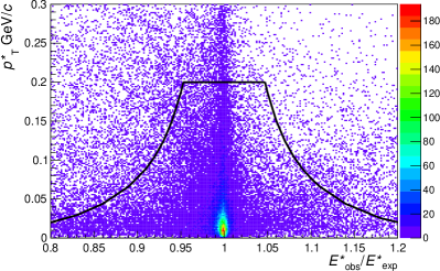
Figure 2: $p^{*}_{T}$ vs. $E^{*}_{\rm obs}/E^{*}_{\rm exp}$ distribution (MC events). The (black) line shows the selection criteria applied to $p^{*}_{T}$ and $E^{*}_{\rm obs}/E^{*}_{\rm exp}$; events below the line are accepted.

A non-signal event imitates $X(3915)$ if a $\psi(2S)$ is produced by a virtual photon from internal bremsstrahlung and if it accompanies either a $\pi^{0}$ or a fake $\pi^{0}$ and also the $\pi^{+}\pi^{-}\pi^{0}$ combination satisfies the $\omega$-mass condition. To suppress this background, we reject the event having the invariant mass of $J/\psi\pi^{+}\pi^{-}$ in the $\psi(2S)$ window [3.6806 GeV/$c^{2}$; 3.6914 GeV/$c^{2}$]. This window is defined as $\pm 2\sigma$ of the $\psi(2S)$ mass resolution. The mass resolutions of $\psi(2S)$(= $J/\psi\pi^{+}\pi^{-}$) and $X(3915)$(= $J/\psi\pi^{+}\pi^{-}\pi^{0}$) are approximately 2.7 MeV/$c^{2}$.

V Results

V.1 Signals and backgrounds

Figure 3 shows the $Q^{2}$ vs. $M(J/\psi\omega)$ distribution from the selected data. Here, $Q^{2}$ is calculated by $Q^{2}=2(p_{\rm beam}p_{\rm tag}-m_{e}^{2})$, where $p_{\rm beam}$ and $p_{\rm tag}$ are the four-momenta of the beam $e^{\pm}$ and tagging $e^{\pm}$, respectively, and $m_{e}$ is the electron mass. The events fall into three classes: a cluster in the $X(3915)$ mass region with $Q^{2}$ less than 10 (GeV/$c$)², a high $Q^{2}$ event at $Q^{2}\approx 30$ (GeV/$c$)², and a high $M$ event at $M\approx 4.08$ GeV/$c^{2}$. In the small $Q^{2}$ region, the detection efficiency diminishes due to the electron tagging condition [see Appendix, Fig. 8]. This region, $Q^{2}<1.5$ (GeV/$c$)², is hatched in Fig. 3, where the detection efficiency falls below 15% of its plateau value.

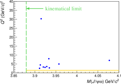
Figure 3: $Q^{2}$ vs. $M(J/\psi\omega)$ distribution from data. The dashed (green) line indicates the kinematical limit: 3.8795 GeV/$c^{2}$. The hatched (orange) region has detection efficiency below 15% of its plateau value as explained in the text.

To derive the numbers of signal and background events, we fit a combination of the threshold-corrected relativistic Breit–Wigner (BW) function and a constant to the $M(J/\psi\omega)$ distribution. The threshold-corrected BW function, $f_{\rm BW}(W)$, is

$${\displaystyle f_{\rm BW}(W)=\frac{\alpha M^{2}\Gamma^{\prime}}{(W^{2}-M^{2})^{2}+M^{2}\Gamma^{\prime 2}}}$$ (2)

where $M$ is the resonance mass, $\alpha$ is a dimensionless normalization factor, and $\Gamma^{\prime}$ is the threshold-corrected resonance width defined by

$${\displaystyle\Gamma^{\prime}=\Gamma\cdot\frac{\rho(W)}{\rho(M)}}$$ (3)

where $\Gamma$ is the resonance width, $\rho(W)$ is the phase space factor for $W$, which is

$${\displaystyle\rho(W)=\frac{1}{16\pi}\frac{\lambda^{1/2}(W^{2},m_{J}^{2},m_{\omega}^{2})}{W^{2}}}$$ (4)

and $\lambda$ is the Källén function [7, 35]. It is defined as

$$\begin{array}[]{l}{\displaystyle\lambda^{1/2}(W^{2},m_{J/\psi}^{2},m_{\omega}^{2})}\\ {\displaystyle=\sqrt{(m_{J/\psi}^{2}+m_{\omega}^{2}-W^{2})^{2}-4m_{J/\psi}^{2}m_{\omega}^{2}}}\end{array}$$ (5)

where $m_{J/\psi}$ is the mass of $J/\psi$(= 3.0969 GeV/$c^{2}$) and $m_{\omega}$ that of $\omega$(= 0.78265 GeV/$c^{2}$) [8]. In the fit, we set $M=3.918$ GeV/$c^{2}$, $\Gamma=0.020$ GeV/$c^{2}$ [8], and $\alpha=2/\pi$, with the fit function (modified BW combined with a flat component)

$${\displaystyle f_{\rm BW+flat}=a_{\rm BW}\cdot f_{\rm BW}+a_{\rm flat},}$$ (6)

where the fit parameters $a_{\rm BW}$ and $a_{\rm flat}$ are the magnitudes of the BW and the flat component, respectively. We ignore a possible distortion of the fit distribution due to the energy dependence of the detection sensitivity, because the effect is small. Energy dependence of the detection sensitivity for $J/\psi\omega$, which is defined by the production of detection efficiency times luminosity function, is estimated as $0.1\Delta W$ %, where $\Delta W$ is in the MeV unit. We use the ROOT/MINUIT implementation of the binned maximum-likelihood method with a 5 MeV/$c^{2}$ bin width and perform the fit in the $M(J/\psi\omega)$ range of [3.880 GeV/$c^{2}$; 4.100 GeV/$c^{2}$]. The units of $f_{\rm BW+flat}$ and $f_{\rm BW}$ are events/(5 MeV/$c^{2}$) and (GeV/$c^{2}$)^-1, respectively. The result of the fit is shown in Fig. 4.

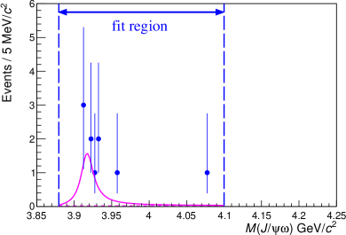
Figure 4: $M(J/\psi\omega)$ distribution with the Breit–Wigner + flat function fit. Abscissa is $M(J/\psi\omega)$ in GeV/$c^{2}$. Ordinate is the number of events per 5 MeV/$c^{2}$. Solid (magenta) curve shows the result of the fit. Horizontal dashed (magenta) line shows the flat component. Vertical dashed (blue) lines indicate the fit region.

The obtained parameters are $a_{\rm BW}=0.049\pm 0.018$ GeV/$c^{2}$/(5 MeV/$c^{2}$) and $a_{\rm flat}=0.022\pm 0.035$ /(5 MeV/$c^{2}$). The number of signal events is $n_{\rm sig}=9.0\pm 3.2$, obtained by integrating $f_{\rm BW}$ with $a_{\rm BW}$ over the fit region [3.8795 GeV/$c^{2}$; 4.1000 GeV/$c^{2}$]. The number of background events is $n_{\rm bg}^{\rm fit}=0.3\pm 0.4$, calculated for the $X(3915)$ band, which we define 60 MeV/$c^{2}$. It is obtained by multiplying $a_{\rm flat}$ by the ratio of the $X(3915)$ band width, 60 MeV/$c^{2}$, to the bin width, 5 MeV/$c^{2}$.

To confirm the number of background events, it is also derived using the number of events in the $\omega$ sidebands. Figure 5 shows the $M(\pi^{+}\pi^{-}\pi^{0})$ vs. $M(J/\psi\pi^{+}\pi^{-}\pi^{0})$ distribution. The sideband regions are set as two rectangles with heights $M(\pi^{+}\pi^{-}\pi^{0})$ in [0.60,0.70] GeV/$c^{2}$ and [0.83,0.93] GeV/$c^{2}$ and the width $M(J/\psi\pi^{+}\pi^{-}\pi^{0})$ in [3.88,4.10] GeV/$c^{2}$. There are in total four events in the $\omega$ sideband rectangles. For the signal region, a rectangle of 0.080 GeV/$c^{2}$ high in $M(\pi^{+}\pi^{-}\pi^{0})$ and 0.060 GeV/$c^{2}$ wide in $M(J/\psi\pi^{+}\pi^{-}\pi^{0})$ is used. From this, the obtained number of background events is $n_{\rm bg}^{\omega}=0.4\pm 0.3$. As $n_{\rm bg}^{\omega}$ is calculated using non-$\omega$ events while $n_{\rm bg}^{\rm fit}$ is obtained from identified $\omega$ events, the contents in the samples are different. Nevertheless, the results from the two methods are approximately the same. We use a conservative number: $n_{\rm bg}=0.4\pm 0.4$. The resulting signal significance for nine observed events is then 5.6$\sigma$.

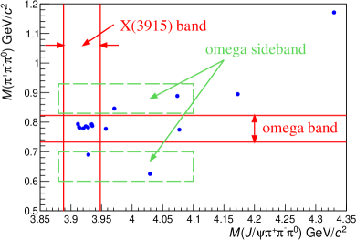
Figure 5: $M(\pi^{+}\pi^{-}\pi^{0})$ vs. $M(J/\psi\pi^{+}\pi^{-}\pi^{0})$ distribution to estimate the background rate using $\omega$ sideband events. Dashed (green) rectangles show the $\omega$ sidebands. Horizontal (red) line pair shows the $\omega$ signal band. Vertical (red) line-pair shows the $X(3915)$ signal band.

The measured number of signals is compared to the expectation, $n_{\rm sig}^{\rm exp}$, derived from the existing no-tag two-photon measurement [8, 7]. For this, we use the spin-parity of $X(3915)$ as $J^{P}=0^{+}$ and use Eqs. (15) and (19) from the SBG model to extrapolate the $Q^{2}=0$ value, $\Gamma_{\gamma\gamma}(0){\cal B}(X\rightarrow J/\psi\omega)=(54\pm 9)$ eV/$c^{2}$ [8, 7], to higher $Q^{2}$, where $\Gamma_{\gamma\gamma}(0)$ is the $\gamma\gamma$ decay width of $X(3915)$ at $Q^{2}=0$ and ${\cal B}(X\rightarrow J/\psi\omega)$ is the branching fraction of $X(3915)$ decaying to $J/\psi\omega$. The result is $n_{\rm sig}^{\rm exp}=4.1\pm 0.7$. For a different prediction, if we assume the spin-parity as $J^{P}=2^{+}$, the expectation is $7.5\pm 1.3$ events using $\Gamma_{\gamma\gamma}(0){\cal B}(X\rightarrow J/\psi\omega)=16$ eV in Ref. [3] with the $J=2$ SBG model, Eq. (20), assuming $\epsilon=1.0$.

V.2 Q² distribution

To determine the $Q^{2}$ distribution, we must first determine the treatment of the two outlier events in Fig. 3. The event at $M\approx 4.08$ GeV/$c^{2}$ is excluded because it is far outside the $X(3915)$ region. The event at $Q^{2}\approx 30$ (GeV/$c$)² is discussed in the following.

Figure 6(a) shows the $M(\pi^{+}\pi^{-}\pi^{0})$ vs. $M(J/\psi\pi^{+}\pi^{-})$ distribution, applying neither the $\omega$ selection nor the $\psi(2S)$ veto. The high-$Q^{2}$ event is located at 0.9 MeV/$c^{2}$ above the upper boundary of the $\psi(2S)$ veto. There are six events in the $\psi(2S)$ veto. Of the six events, two pass the $\omega$ selection. Figure 6(b) shows the $Q^{2}$ vs. $M(J/\psi\pi^{+}\pi^{-})$ distribution. The two $\psi(2S)$-vetoed events, in addition to the high-$Q^{2}$ event, have high $Q^{2}$s: $Q^{2}>10$ (GeV/$c$)². All the other events that pass the $\psi(2S)$ veto have a lower $Q^{2}$, i.e., $Q^{2}<10$ (GeV/$c$)². From this we conclude that $\psi(2S)$-vetoed events have significantly higher $Q^{2}$ than the $X(3915)$ events.

As for the possibility of the high-$Q^{2}$ event being an $X(3915)$ signal, the Belle experiment had little sensitivity to measure single-tag two-photon events with $Q^{2}$ around 30 (GeV/$c$)² as detailed in the Appendix (see, e.g., Fig. 9). Hence, it is improbable for the high-$Q^{2}$ event to be a single-tag two-photon event.

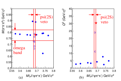
Figure 6: (a) $M(\pi^{+}\pi^{-}\pi^{0})$ vs. $M(J/\psi\pi^{+}\pi^{-})$ and (b) $Q^{2}$ vs. $M(J/\psi\pi^{+}\pi^{-})$ distributions. Star (red): high-$Q^{2}$ event. Open circles (blue): $\psi(2S)$-vetoed events. Closed circles (blue): $X(3915)$ candidates. (a) neither $\omega$ selection nor $\psi(2S)$ veto are applied. (b) events pass the $\omega$ selection but no $\psi(2S)$ veto is applied. Vertical red lines indicate the $\psi(2S)$-veto window; the horizontal red lines in panel (a) are the $\omega$ signal band.

To estimate the probability of having one $\psi(2S)\pi^{0}$ event in the region adjacent to the $\psi(2S)$ veto window, where the high-$Q^{2}$ event is located, we estimate the probability of $\psi(2S)$ events escaping the veto and having a $\pi^{0}$. For this, we employ the data sample used in the $X(3872)$ search and examine the $M(J/\psi\pi^{+}\pi^{-})$ distribution [34]. There are 231 events in the $\psi(2S)$-veto window of $\pm 5.4$ MeV/$c^{2}$ used in the current study. There are 12 events in the 2.7 MeV bin, adjacent to the upper boundary of the veto, where the high-$Q^{2}$ event is located. If we normalize the number of events in the veto window to six that we observe as $\psi(2S)\pi^{0}$s in this study, those 12 events correspond to 0.31 events/bin, or 0.11 events/MeV. As seen in Fig. 6(a), two out of six events are inside the $\omega$ region. Hence, the expected number of veto leaks is 0.04 events/MeV. Then, by assuming the width of the leak region as 2 MeV and the uncertainty in the number of events as 0.1 events, the number of expected events is estimated to be $0.1\pm 0.1$ events. Significance of that number exceeding one event is 1.5 $\sigma$, or 7%.

A possible way of producing $\psi(2S)\pi^{0}$ is by a virtual photon, radiated by internal bremsstrahlung from $e^{-}$ or $e^{+}$, similar to the case of $\psi(2S)$ production. However, there are suppressions to the $\psi(2S)\pi^{0}$ production compared to $\psi(2S)$. The $\psi(2S)$s are produced as resonances, but the $\psi(2S)\pi^{0}$s are not. In order to be $J^{P}=1^{-}$, the $\psi(2S)\pi^{0}$ has to be in a $P$-wave. In addition, $\psi(2S)\pi^{0}$ is an isospin one state. Thus, further suppressions are expected.

In the arguments up to this point, we assume the $\pi^{0}$s as real. However, the reconstructed $\pi^{0}$s can be fake. Using MC events, we observe that 13% of $\pi^{0}$s, found in the $X(3915)$ candidates, are fake. This number is considered a lower limit as we found that the abundance of low-$p_{T}$ $\pi^{0}$s is higher in real data than in MC. Thus, the fraction of fake $\pi^{0}$s is higher at low $p_{T}$ than at high $p_{T}$. The observed $\psi(2S)\pi^{0}/\psi(2S)$ is 6/231, where the $\pi^{0}$s are either real or fake. In summary, it is plausible that the high-$Q^{2}$ event is a $\psi(2S)\pi^{0}$ background.

If we remove the high-$Q^{2}$ event from the $f_{\rm BW+flat}$ fit, the result is $a_{\rm BW}=0.043\pm 0.017$ GeV/$c^{2}$/(5 MeV/$c^{2}$) and $a_{\rm flat}=0.025\pm 0.036$ /(5 MeV/$c^{2}$). From that, we obtain $n_{\rm sig}=7.9^{+3.1}_{-3.0}$. As a note, the significance for eight events is 5.2$\sigma$.

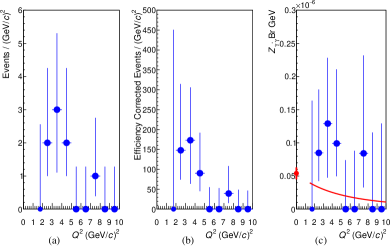
Figure 7: Measured $Q^{2}$ distributions: (a) the number of events per (GeV/$c$)², (b) efficiency corrected number of events per (GeV/$c$)², and (c) $Z_{\gamma^{*}\gamma}{\cal B}(X\rightarrow J/\psi\omega)$. Bin widths of all data are 1 (GeV/$c$)² except the smallest $Q^{2}$ bins whose bin width is 0.5 (GeV/$c$)². The solid (red) curve shows the SBG prediction based on the data of the no-tag two-photon measurement, $\Gamma_{\gamma\gamma}(0){\cal B}(X\rightarrow J/\psi\omega)=54$ eV/$c^{2}$, shown as a small (red) circle.

In the low-$Q^{2}$ region, there are eight events in the $M(J/\psi\pi^{+}\pi^{-}\pi^{0})$ range [3.911 GeV/$c^{2}$; 3.958 GeV/$c^{2}$]. In the following, we will study the $Q^{2}$ structure of $X(3915)$ using these eight events, excluding the high-$Q^{2}$ event and the high-$M$ event, which are considered as backgrounds. Figure 7 shows the $Q^{2}$ distributions for three quantities: the number of events, efficiency corrected number of events, and $Z_{\gamma^{*}\gamma}{\cal B}(X\rightarrow J/\psi\omega)$, where $Z_{\gamma^{*}\gamma}$ is a $Q^{2}$-dependent decay function defined by Eq. (12). The $Z_{\gamma^{*}\gamma}{\cal B}(X\rightarrow J/\psi\omega)$ distribution is obtained by multiplying the event distribution by a correction function further detailed in the Appendix [see Eq. (16)]. The integrated yield of the $Z_{\gamma^{*}\gamma}{\cal B}(X\rightarrow J/\psi\omega)$ distribution in the $Q^{2}$ range of 1.5 (GeV/$c$)² to 10.0 (GeV/$c$)² is $1.9\pm 0.9$ times the expectation from the no-tag measurement, $\Gamma_{\gamma\gamma}(0){\cal B}(X(3915)\rightarrow J/\psi\omega)=54\pm 9$ eV [8, 7], combined with its extrapolation to the higher-$Q^{2}$ region using Eq. (19). The averages, $\langle Q^{2}\rangle$, and the root-mean-squared (rms) values of $Q^{2}$, $\sqrt{\langle(Q^{2}-\langle Q^{2}\rangle)^{2}\rangle}$, for the $Z_{\gamma^{*}\gamma}{\cal B}(X\rightarrow J/\psi\omega)$ distribution are listed in Table 1, both for the measurement and for the SBG model [see Eq. (19) of the Appendix]. They are obtained from the same range in $Q^{2}$ as above, i.e., $1.5~{}(\text{GeV}/c)^{2}\leq Q^{2}\leq 10.0~{}(\text{GeV}/c)^{2}$. The measured average $Q^{2}$, $4.5\pm 0.7$ (GeV/$c$)², agrees with the theoretical prediction, 4.8 (GeV/$c$)². Their difference is approximately 10% of the rms widths of their distributions, which are $1.9\pm 0.8$ (GeV/$c$)² vs. 2.4 (GeV/$c$)². The resolution in $Q^{2}$ is about 0.03 (GeV/$c$)² depending on the tag-electron’s scattering angle. Hence, the measurement is consistent with the prediction both in the averages and the rms values of $Q^{2}$. In summary, the measured $Q^{2}$ distribution does not show a significant shift to lower $Q^{2}$; it agrees with the SBG $c\bar{c}$ model.

Table 1: Comparison of the measurement and the SBG model prediction [20] for the $Q^{2}$ distribution of $Z_{\gamma^{*}\gamma}{\cal B}(X\rightarrow J/\psi\omega)$. $Q^{2}$ resolution is estimated to be about $0.03$ (GeV/$c$)². Used are the eight events shown in Fig. 7.

Item	Measurement	SBG model
Relative yield	$1.9\pm 0.9$	1.0
$\langle Q^{2}\rangle$ (GeV/$c$)2	$4.5\pm 0.7$	4.8
$\sqrt{\langle(Q^{2}-\langle Q^{2}\rangle)^{2}\rangle}$ (GeV/$c$)2	$1.9\pm 0.8$	2.4

VI Systematic Uncertainties

The largest uncertainty is associated with the $\pi^{0}$ selection efficiency, including the rate of fake $\pi^{0}$s. By comparing the number of selected events using the different $\pi^{0}$ selection algorithms, we estimate 15% uncertainty associated with the $\pi^{0}$ selection algorithm. Another uncertainty in $\pi^{0}$ detection is associated to fake $\pi^{0}$s from background photons. In the data before applying $\pi^{0}$ selection, a significant number of low-energy photons, either true or fake, contaminate. These photons can produce fake $\pi^{0}$s. To estimate the effect of such background photons, we look at variations in the ratio of events with identified $\pi^{0}$(s) to all events observed during the whole data-taking period. From this, we estimate a 5.6% uncertainty after correcting the selection efficiency for the events with fake $\pi^{0}$. This effect of background photons is also estimated using MC events simulated with different background conditions, which gives a 3% variation. Conservatively, we use the larger 5.6% as the systematic uncertainty in $\pi^{0}$ identification due to background photons.

Another large uncertainty is associated with $J/\psi$ identification. The combined uncertainty in $J/\psi$ ID is 8%. The largest contribution, 7%, to this comes from the difference in the ratio of the number of $J/\psi$ selected events, $N(J/\psi\rightarrow e^{+}e^{-})/N(J/\psi\rightarrow\mu^{+}\mu^{-})$, between the real data and MC. The other smaller contributions are the uncertainties in the efficiencies of electron and muon IDs, background levels and radiative $\gamma$ corrections in the case of $J/\psi\rightarrow e^{+}e^{-}$ and the shapes of the invariant-mass distributions. They are estimated by the differences in the efficiencies between the real data and MC by varying the selection conditions.

The uncertainties in electron tagging, 5%, and charged pion ID, 3%, are estimated by the difference in the efficiencies between real data and MC by varying the selection conditions. To calculate the detection efficiency, we set the fit region for selecting signal events. Because of the uncertainty in the $X(3915)$ distribution at or near the lower boundary of the fit region, 3.888 GeV/$c^{2}$, detection efficiency will have an uncertainty, which is estimated to be 3%. The uncertainties in the $\omega$ selection, 2%, and the $p_{T}$-and-$E_{\rm obs}^{*}/E_{\rm exp}^{*}$ selection specified by Eq. (1), 4%, are estimated using MC by varying selection condition. The uncertainty in the luminosity function, which is defined by Eq. (9), 3%, is estimated from the uncertainties in QED modeling and numerical integration. The other uncertainties are 2% for missing $p_{T}$, 2% for $||\phi({\rm tag})-\phi({\rm rest})|-\pi|$, 1.8% for track finding, 1.4% for luminosity measurement, 1% for $p_{T}<0.2$ GeV/$c$, 1% for $Q^{2}$ numerical integration, 1% for energy dependence in the detection efficiency, and 0.6% for MC statistics.

Table 2 lists a summary of systematic uncertainties. As a total, combined quadratically, uncertainty in the reconstruction efficiency is 20%.

Table 2: Breakdown of contributions to the systematic uncertainty in the reconstruction efficiency.

Item	Uncertainty
$\pi^{0}$ selection algorithm	15%
$J/\psi$ ID	8%
Fake $\pi^{0}$ by background	5.6%
Electron tagging	5%
$p_{T}$-and-$E^{*}_{\rm obs}/E^{*}_{\rm exp}$ selection	4%
Charged pion ID	3%
Luminosity function	3%
Efficiency window	3%
$\omega$ selection	2%
Missing $p_{T}$	2%
$||\phi({\rm tag})-\phi({\rm rest})|-\pi|$	2%
Luminosity measurement	1.4%
Track finding	1.8%
$p_{T}<0.2$ GeV/$c$	1%
$Q^{2}$ numerical integration	1%
Energy dependence in efficiency	1%
MC statistics	0.6%
Total	20%

VII Summary

We performed the first measurement of the $Q^{2}$ distribution of $X(3915)$ production in single-tag two-photon interactions. For signals, $7.9\pm 3.1({\rm stat.})\pm 1.5({\rm syst.})$ events are observed, while the expectation is $4.1\pm 0.7$, derived from the measured decay width at $Q^{2}=0$, $\Gamma_{\gamma\gamma}(0){\cal B}(X\rightarrow J/\psi\omega)=54\pm 9$ eV, extrapolated to higher $Q^{2}$ region using the SBG $c\bar{c}$ model [20]. The shape of the $Q^{2}$ distribution is also consistent with this model. These results can be used to constrain non-$c\bar{c}$ models of the $X(3915)$ when predictions for the $Q^{2}$ distribution become available.

Appendix A DIFFERENTIAL CROSS SECTION

The $Q^{2}$-differential $X(3915)$-production cross section in single-tag two-photon interactions is given by

$$\begin{array}[]{l}{\displaystyle\frac{d\sigma_{ee}(X(3915))}{dQ^{2}}=2\cdot 2\pi^{2}\frac{(2J+1)\,2\Gamma_{\gamma\gamma}(0)}{M^{2}}}\\ {\displaystyle\times\left[f_{TT}(Q^{2},M^{2})\frac{d^{2}L^{TT}_{\gamma^{*}\gamma}}{dWdQ^{2}}\right.}\\ \lx@intercol\hfil\displaystyle\left.\left.+f_{LT}(Q^{2},M^{2})\frac{d^{2}L^{LT}_{\gamma^{*}\gamma}}{dWdQ^{2}}\right]\right|_{W=M}\lx@intercol\end{array}$$ (7)

where the factor 2 in the front stems from the two tag conditions ($e^{-}$-tag and $e^{+}$-tag), $J$ is the $X(3915)$ spin, $\Gamma_{\gamma\gamma}(0)$ is the $\gamma\gamma$ decay width of $X(3915)$ at $Q^{2}=0$, $M$ is the mass of the $X(3915)$, and $W$ is the energy of the two-photon system in its rest frame. Furthermore, $f_{TT}(Q^{2},M^{2})$ and $f_{LT}(Q^{2},M^{2})$ are the form factors for $X(3915)$ production in interactions of two transverse (virtual and quasireal) photons and of one longitudinal (virtual) and one transverse (quasireal) photon, respectively; $L^{TT}_{\gamma^{*}\gamma}$ as well as $L^{LT}_{\gamma^{*}\gamma}$ are the luminosity functions for the case of two transverse photons and for the case of one longitudinal and one transverse photon, respectively.

Defining

$$\epsilon = {\displaystyle\frac{L^{LT}_{\gamma^{*}\gamma}}{L^{TT}_{\gamma^{*}\gamma}}}$$ (8)

$$L_{\gamma^{*}\gamma} = {\displaystyle L^{TT}_{\gamma^{*}\gamma}}$$ (9)

and

$${\displaystyle f(Q^{2},M^{2},\epsilon)=f_{TT}(Q^{2},M^{2})+\epsilon f_{LT}(Q^{2},M^{2}),}$$ (10)

Eq. (7) can be rewritten as

$$\begin{array}[]{l}{\displaystyle\frac{d\sigma_{ee}(X)}{dQ^{2}}}\\ {\displaystyle=8\pi^{2}\frac{(2J+1)\Gamma_{\gamma\gamma}(0)}{M^{2}}f(Q^{2},M^{2},\epsilon)\left.\frac{d^{2}L_{\gamma^{*}\gamma}}{dWdQ^{2}}\right|_{W=M}.}\end{array}$$ (11)

We further introduce a $Q^{2}$-dependent decay function,

$${\displaystyle Z_{\gamma^{*}\gamma}(Q^{2},M^{2},\epsilon)=\frac{f(Q^{2},M^{2},\epsilon)\Gamma_{\gamma\gamma}(0)}{(1+Q^{2}/M^{2})}\,,}$$ (12)

and rewrite Eq. (11) as

$$\begin{array}[]{lll}{\displaystyle\frac{d\sigma_{ee}(X)}{dQ^{2}}}&=&{\displaystyle 8\pi^{2}\frac{(2J+1)(1+Q^{2}/M^{2})}{M^{2}}Z_{\gamma^{*}\gamma}(Q^{2},M^{2},\epsilon)}\\ &&{\displaystyle\times\left.\frac{d^{2}L_{\gamma^{*}\gamma}}{dWdQ^{2}}\right|_{W=M}.}\end{array}$$ (13)

The differential event-yield distribution is

$${\displaystyle\frac{dN_{ee}(X)}{dQ^{2}}} = {\displaystyle\frac{d\sigma_{ee}(X)}{dQ^{2}}\varepsilon_{\rm eff}(Q^{2})L_{\rm int}{\cal B}(X\rightarrow J/\psi\omega)}$$ (15)

$${\displaystyle\times\,{\cal B}(J/\psi\rightarrow\ell^{+}\ell^{-}){\cal B}(\omega\rightarrow\pi^{+}\pi^{-}\pi^{0})\,,}$$

$$= {\displaystyle\,8\pi^{2}\frac{(2J+1)(1+Q^{2}/M^{2})}{M^{2}}Z_{\gamma^{*}\gamma}(Q^{2},M^{2},\epsilon)}$$

$${\displaystyle\times\,\varepsilon_{\rm eff}(Q^{2})L_{\rm int}\left.\frac{d^{2}L_{\gamma^{*}\gamma}}{dWdQ^{2}}\right|_{W=M}}$$

$${\displaystyle\times\,{\cal B}(X\rightarrow J/\psi\omega)\,{\cal B}(J/\psi\rightarrow\ell^{+}\ell^{-})}$$

$${\displaystyle\times\,{\cal B}(\omega\rightarrow\pi^{+}\pi^{-}\pi^{0})\,,}$$

where $L_{\rm int}$ is the integrated luminosity, ${\cal B}(J/\psi\rightarrow\ell^{+}\ell^{-})$ is the branching fraction of $J/\psi$ decaying to either an electron pair or a muon pair, ${\cal B}(\omega\rightarrow\pi^{+}\pi^{-}\pi^{0})$ is the branching fraction of $\omega$ decaying to three pions. Rearranging Eq. (15), one can relate $Z_{\gamma^{*}\gamma}(Q^{2},M^{2},\epsilon)\,{\cal B}(X\rightarrow J/\psi\omega)$ to the event-yield distribution:

$$Z_{\gamma^{*}\gamma}(Q^{2},M^{2},\epsilon){\cal B}(X\rightarrow J/\psi\omega)=C(Q^{2},M^{2})\frac{dN_{ee}(X)}{dQ^{2}}$$ (16)

with

$$\begin{array}[]{l}{\displaystyle 1/C(Q^{2},M^{2})}\\ {\displaystyle=8\pi^{2}\frac{(2J+1)(1+Q^{2}/M^{2})}{M^{2}}\left.\frac{d^{2}L_{\gamma^{*}\gamma}}{dWdQ^{2}}\right|_{W=M}}\\ {\displaystyle\ \ \ \times\,\varepsilon_{\rm eff}(Q^{2})\,L_{\rm int}\,{\cal B}(J/\psi\rightarrow\ell^{+}\ell^{-})\,{\cal B}(\omega\rightarrow\pi^{+}\pi^{-}\pi^{0})\,.}\end{array}$$ (17)

For the production of $J^{P}=0^{+}$ particles, as $X(3915)$, the $f_{LT}$ component does not contribute and hence the $\epsilon$ dependence of $Z_{\gamma^{*}\gamma}$ drops out. Furthermore, with $J=0$ and using the integrated luminosity in this analysis, $L_{\rm int}=825~{}\text{fb}^{-1}$, as well as ${\cal B}(J/\psi\rightarrow\ell^{+}\ell^{-})=0.11932$ and ${\cal B}(\omega\rightarrow\pi^{+}\pi^{-}\pi^{0})=0.892$ [7], Eq. (17) simplifies to

$$\begin{array}[]{lcl}1/C(Q^{2},M^{2})&=&{\displaystyle 8\pi^{2}\frac{1+Q^{2}/M^{2}}{M^{2}}}\\ &&{\displaystyle\times\,3.418\times 10^{13}\varepsilon_{\rm eff}(Q^{2})\!\left.\frac{d^{2}L_{\gamma^{*}\gamma}}{dWdQ^{2}}\right|_{W=M}\!\!.}\end{array}$$ (18)

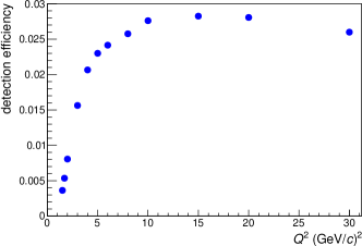
Figure 8: Detection efficiency as a function of $Q^{2}$ as obtained from a MC simulation.

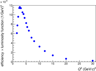
Figure 9: Detection efficiency times luminosity function as a function of $Q^{2}$. Ordinate is $\left.\varepsilon_{\rm eff}(Q^{2})\frac{d^{2}L_{\gamma^{*}\gamma}}{dWdQ^{2}}\right|_{W=M}$ (1/GeV)³.

In order to obtain numerical values for $C(Q^{2},M^{2})$, the detection efficiency is calculated using MC events. Figure 8 shows the resulting efficiency as a function of $Q^{2}$. The product of the efficiency and the luminosity function is presented in Figure 9. This distribution shows our sensitivity for measuring the $Q^{2}$ distribution; the sensitive region is between $Q^{2}=1.5$ (GeV/$c$)² and $Q^{2}\approx 10$ (GeV/$c$)². Finally, numerical values for $C(Q^{2},M^{2})$ for $M=3.918$ GeV/$c^{2}$ are listed in Table 3.

Table 3: $C(Q^{2},M^{2})$: conversion factor from the number of events to $Z_{\gamma^{*}\gamma}(Q^{2}/M^{2}){\cal B}(X\rightarrow J/\psi\omega)$ as a function of $Q^{2}$.

$Q^{2}$ (GeV/$c$)2	1.5	1.7	2.0	2.4	2.6	3.0	3.6
$C(Q^{2},M^{2})$ $\times 10^{-8}$	8.49	6.62	5.25	4.31	4.18	4.18	4.38
$Q^{2}$ (GeV/$c$)2	4.0	4.4	5.0	5.4	6.0	7.0	8.0
$C(Q^{2},M^{2})$ $\times 10^{-8}$	4.44	4.74	5.21	5.69	6.17	7.59	8.51
$Q^{2}$ (GeV/$c$)2	10.0	12.0	15.0	20.0	30.0
$C(Q^{2},M^{2})$ $\times 10^{-8}$	10.62	13.90	20.82	37.58	80.09

The theoretical expression for the decay function $Z_{\gamma^{*}\gamma}$ is given in the SBG model [20] as

$$Z_{\gamma^{*}\gamma}(Q^{2}/M^{2})=\frac{1}{(1+Q^{2}/M^{2})^{4}}\left(1+\frac{Q^{2}}{3M^{2}}\right)^{2}\Gamma_{\gamma\gamma}(0)$$ (19)

for $J^{P}=0^{+}$, while it is

$$\begin{array}[]{l}{\displaystyle Z_{\gamma^{*}\gamma}(Q^{2}/M^{2},\epsilon)}\\ {\displaystyle=\frac{1}{(1+Q^{2}/M^{2})^{4}}\left(1+\frac{Q^{4}}{6M^{4}}+\epsilon\frac{Q^{2}}{M^{2}}\right)\Gamma_{\gamma\gamma}(0)}\end{array}$$ (20)

in case of $J^{P}=2^{+}$.

References

- S.-K. Choi et al. [2003] S.-K. Choi et al. (Belle Collaboration), Phys. Rev. Lett. 91, 262001 (2003).
- S.-K. Choi et al. [2005] S.-K. Choi et al. (Belle Collaboration), Phys. Rev. Lett. 94, 182002 (2005).
- S. Uehara et al. [2010] S. Uehara et al. (Belle Collaboration), Phys. Rev. Lett. 104, 092001 (2010).
- B. Aubert et al. [2008a] B. Aubert et al. (BABAR Collaboration), Phys. Rev. Lett. 101, 082001 (2008a).
- J. P. Lees et al. [2012] J. P. Lees et al. (BABAR Collaboration), Phys. Rev. D 86, 072002 (2012).
- Note [1] Charge-conjugate process will be implicitly included.
- R. L. Workman et al. [2022] R. L. Workman et al. (Particle Data Group), Prog. Theor. Exp. Phys. 2022, 083C01 (2022).
- P. A. Zyla et al. [2020] P. A. Zyla et al. (Particle Data Group), Prog. Theor. Exp. Phys. 2020, 083C01 (2020), 2021 update.
- Z.-Y. Zhou, Z. Xiao and H.-Q. Zhou [2015] Z.-Y. Zhou, Z. Xiao and H.-Q. Zhou, Phys. Rev. Lett. 115, 022001 (2015).
- R. Aaij et al. [2020] R. Aaij et al. (LHCb Collaboration), Phys. Rev. D 102, 112003 (2020).
- Note [2] Kinematically allowed decay is only if the mass is 3.920 GeV/ and . Also in , no peak is seen.
- T. Aushev et al. [2010] T. Aushev et al. (Belle Collaboration), Phys. Rev. D 81, 031103 (2010).
- B. Aubert et al. [2008b] B. Aubert et al. (BABAR Collaboration), Phys. Rev. D 77, 011102 (2008b).
- J. Brodzicka et al. [2008] J. Brodzicka et al. (Belle Collaboration), Phys. Rev. Lett. 100, 092001 (2008).
- S. L. Olsen [2015] S. L. Olsen, Phys. Rev. D 91, 057501 (2015).
- R. F. Lebed and A. D. Polosa [2016] R. F. Lebed and A. D. Polosa, Phys. Rev. D 93, 094024 (2016).
- A. M. Badalian and Yu. A. Simnov [2022] A. M. Badalian and Yu. A. Simnov, Eur. Phys. J. C 82, 1024 (2022).
- X. Li and M. B. Voloshin [2015] X. Li and M. B. Voloshin, Phys. Rev. D 91, 114014 (2015).
- Y. Yamaguchi, A. Hosaka, S. Takeuchi, and M. Takizawa [2020] Y. Yamaguchi, A. Hosaka, S. Takeuchi, and M. Takizawa, J. Phys. G: 47, 053001 (2020).
- G. A. Schuler, F. A. Berends, and R. van Gulik [1998] G. A. Schuler, F. A. Berends, and R. van Gulik, Nucl. Phys. B523, 423 (1998).
- S. Kurokawa and E. Kikutani [2003] S. Kurokawa and E. Kikutani, Nucl. Instrum. Methods Phys. Res., Sect. A 499, 1 (2003).
- T. Abe et al. [2013] T. Abe et al. (KEKB), Prog. Theor. Exp. Phys. 2013, 03A001 (2013).
- A. Abashian et al. [2002a] A. Abashian et al. (Belle Collaboration), Nucl. Instrum. Methods Phys. Res., Sect. A 479, 117 (2002a).
- J. Brodzicka et al. [2012] J. Brodzicka et al. (Belle Collaboration), Prog. Theor. Exp. Phys. 2012, 04D001 (2012).
- M. Masuda et al. [2016] M. Masuda et al. (Belle Collaboration), Phys. Rev. D 93, 032003 (2016).
- [26] S. Uehara, KEK Report No. 96-11, 1996, arXiv:1310.0157/[hep-ph] .
- Note [3] .
- E. Barberio, B. van Eijk and Z. Wa̧s [1991] E. Barberio, B. van Eijk and Z. Wa̧s, Comput. Phys. Commun. 66, 115 (1991).
- E. Barberio and Z. Wa̧s [1994] E. Barberio and Z. Wa̧s, Comput. Phys. Commun. 79, 291 (1994).
- [30] R. Brun et al., Report No. CERN DD/EE/ 84-1, 1987.
- K. Hanagaki et al. [2002] K. Hanagaki et al., Nucl. Instrum. Methods Phys. Res., Sect. A 485, 490 (2002).
- A. Abashian et al. [2002b] A. Abashian et al., Nucl. Instrum. Methods Phys. Res., Sect. A 491, 69 (2002b).
- E. Nakano [2002] E. Nakano, Nucl. Instrum. Methods Phys. Res., Sect. A 494, 402 (2002).
- Y. Teramoto et al. [2021] Y. Teramoto et al. (Belle Collaboration), Phys. Rev. Lett. 126, 122001 (2021).
- G. Källén [1964] G. Källén, Elementary Particle Physics (Addison-Wesley Publ. Co., New York, 1964).