Efficient Encoders for Streaming Sequence Tagging

Abstract

A naive application of state-of-the-art bidirectional encoders for streaming sequence tagging would require re-encoding all tokens from scratch whenever a new token appears in an incremental streaming input (like transcribed speech). The lack of re-usability of previous computation leads to a higher number of Floating Point Operations (or FLOPs) and higher number of unnecessary label flips. Increased FLOPs consequently lead to higher wall-clock time and increased label flipping leads to poorer streaming performance. In this work, we present Hybrid Encoder with Adaptive Restart (HEAR) that addresses these issues while maintaining the performance of bidirectional encoders over offline (or complete) inputs and improving performance on streaming (or incomplete) inputs. HEAR uses a Hybrid unidirectional-bidirectional encoder architecture to perform sequence tagging, along with an Adaptive Restart Module (ARM) to selectively guide the restart of bidirectional portion of the encoder. Across four sequence tagging tasks, HEAR offers FLOPs savings in streaming settings upto 71.1% and also outperforms bidirectional encoders for streaming predictions by upto +10% streaming exact match.

1 Introduction

State-of-the-art text encoding methods assume the offline setting, where the entire input text is available when encoding it. This differs from the streaming setting where the input text grows over time (such as transcribed speech or a typed query) Cho and Esipova (2016); Gu et al. (2017); Chang et al. (2022). Processing streaming input incrementally can enable suggestions on partial inputs Iranzo Sanchez et al. (2022), reduced final latency Zhou et al. (2022) and lead to more interactive NLU agents Cai and de Rijke (2016).

Model	GFLOPs	Offline F1	Streaming EM
BiDi encoder	74.7	93.1	75.1
Hybrid encoder	43.4	93.0	72.5
HEAR (Hybrid + ARM)	21.6	93.0	85.1

Table 1: Computation cost (Giga FLOPs), Offline F1 and Streaming Exact Match accuracy of standard bidirectional (BiDi) encoder, Hybrid encoder model and HEAR (Hybrid encoder with ARM for guiding Adaptive Restarts) on SNIPS test set.

Existing state-of-the-art bidirectional encoders (such as Devlin et al. (2019)) are computationally expensive for streaming processing. When a new token is received, these models require a restart, i.e., re-computation of representation of each token by re-running the bidirectional layer Kahardipraja et al. (2021). This adds to the computational cost (i.e., Higher FLOPs) during streaming and leads to higher wall clock time. Another limitation of these encoders is poorer generalization to partial inputs Madureira and Schlangen (2020), stemming from these models being trained only on complete (and offline) inputs. Despite these disadvantages, such bidirectional models offer better offline performance than unidirectional models across several NLP tasks like sequence tagging Kahardipraja et al. (2021).

We address these issues by proposing HEAR – Hybrid Encoder with Adaptive Restarts, where a separate Adaptive Restart Module (ARM) predicts when to restart the encoder. The encoder in HEAR is a Hybrid encoder that reduces the computational cost of running the models in streaming settings. In a Hybrid encoder, the earlier layers are unidirectional and the deeper layers are bidirectional. This design allows early contextualization, and limits the need for restart to the later layers. While Hybrid encoder reduce streaming computational overhead, restarting them at every new token may not be required. Thus, we propose a lightweight Adaptive Restart Module (ARM) to guide restarts, by predicting whether restarting the bidirectional layers of the Hybrid encoder will benefit the model performance. This module is also compatible with fully bidirectional encoders.

Table 1 showcases the strength of HEAR on one of the sequence tagging dataset we consider. In terms of streaming computation, measured in terms of FLOPs (lower is better), Hybrid encoder offers significant saving from purely bidirectional (BiDi) encoders and FLOPs savings improve upon incorporating ARM in HEAR. In terms of offline performance, Hybrid encoder and HEAR achieves parity with BiDi encoders and in terms of streaming performance, HEAR significantly outperforms BiDi encoders.

Following are our key contributions:

• We introduce Hybrid encoder for computationally cheaper streaming processing (§3.1), that maintains the offline F1 score of bidirectional encoders, while reducing FLOPs by an average of 40.2% across four tasks.

• We propose the ARM module (§3.2) to decide when to restart. The ARM reduces FLOP of Hybrid encoder by 32.3% and improves streaming predictions by +4.23 Exact Match.

• Our best model HEAR combines Hybrid encoder with ARM (§5) to achieve strong streaming performance while saving FLOPs and offering competitive offline performance across four sequence tagging tasks.

2 Streaming Sequence Tagging

In the streaming sequence tagging task, we assume that at time $1\leq t\leq n$, we have received the first $t$ tokens $\mathbf{x}_{t}=(x_{1},\cdots x_{t})$ as input from a stream of transcribed speech or user-typed input. The model then predicts the tags for all $t$ tokens $\hat{\mathbf{y}}_{t}=(\hat{y}_{1,t},\hat{y}_{2,t}\cdots\hat{y}_{t,t})$. The models predictions $\hat{\mathbf{y}}_{n}$ over the offline input $\mathbf{x}=\mathbf{x}_{n}$ is the offline tag sequence prediction which is evaluated against the ground truth $\mathbf{y}^{*}_{n}=(y^{*}_{1},y^{*}_{2}\cdots y^{*}_{n})$. However, in the streaming settings, we are concerned with predicted label sequences over all of the prefixes $\hat{\mathbf{Y}}=(\hat{\mathbf{y}}_{1},\hat{\mathbf{y}}_{2}\cdots\hat{\mathbf{y}}_{n})$.

During training we only have access to the offline ground-truth label sequence over the offline input sequence $\mathbf{y}^{*}_{n}$, even though ground truth labels for tokens may change as additional context is received in the future timesteps.

3 Streaming Sequence Tagging with HEAR

In order to motivate HEAR, consider how existing BiDi encoders would be used in streaming sequence tagging. At time $t$ and the input sequence $\mathbf{x}_{t}$, the model restarts to predicts the label sequence $\hat{\mathbf{y}}_{t}$ i.e. it re-computes all its layers for all tokens, without leveraging any of its previous computation or any previously predicted labels. Consequently, running a typical $O(n^{2})$ encoder would have $O(n^{3})$ computations in streaming settings, over $n$ input tokens. Therefore, naively using existing BiDi encoders for streaming settings is highly inefficient. Previous works tackle inefficiency by modifying the streaming model to infer only once for each word, after $k$ future tokens have been received Oda et al. (2015); Grissom II et al. (2014). This leads to a $k$-delayed output with possibility for revisions after additional future words have been received. However, this may lead to poor performance for tasks involving long-range dependency (e.g., SRL) and a higher output lag.

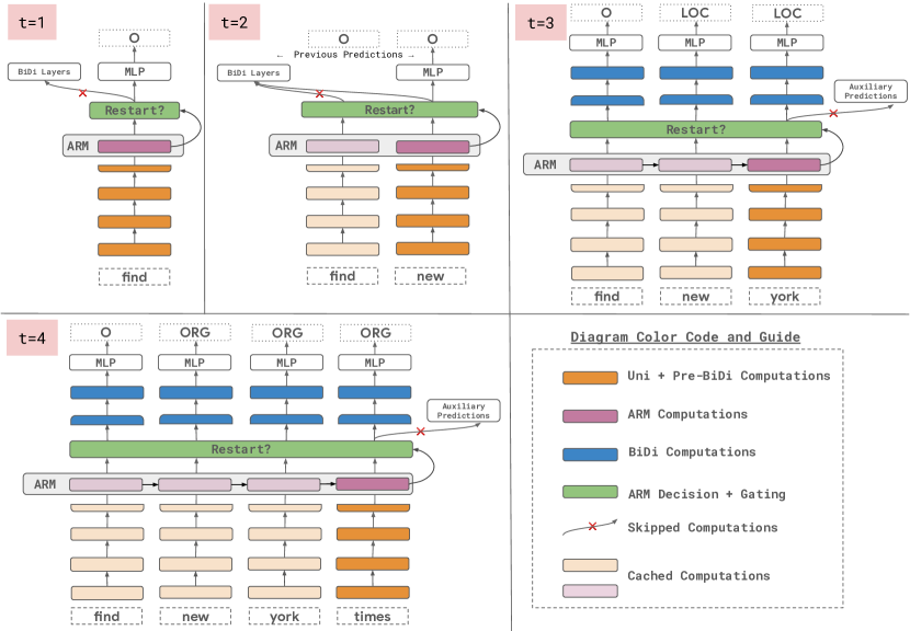
Figure 2: The HEAR model in streaming setting. At $t=1$, ARM decides not to run the bidirectional layers and exit early through the auxiliary predictor over unidirectional encoding. Similarly at $t=2$, ARM decides not to restart and considers the auxiliary predictions of the latest token and the predictions from the previous steps. At $t=3$ and $t=4$, ARM decides to restart and runs the bidirectional layers to get prediction for all the tokens from scratch. Note that in all the steps, for unidirectional layers and ARM, the computation is performed only for the latest token received.

HEAR is a system consisting of a trained Hybrid encoder model and an ARM that is trained over the Hybrid encoder. The early unidirectional layers in Hybrid encoder, reduces the computational cost of restart of the encoder. The ARM guides when to restart the Hybrid encoder. It saves computational cost by keeping the model from restarting at each timestep and also improves streaming performance by avoiding unnecessary label flips stemming from avoidable restarts. Figure 2 shows running of HEAR in streaming settings over an example. For each new token in the streaming input, all the unidirectional layers and a part of first bidirectional layer is ran for the token, to obtain its unidirectional encodings and updated cache. These are then used by ARM to predict whether to restart the bidirectional layer or not. If the bidirectional layer is to be restarted, then we obtain updated labels for all the tokens received in the stream. Otherwise, the auxiliary predictor is ran over the unidirectional encoder for the current token to obtain its label and the labels from previous timestep is copied for all other tokens.

We now formally introduce Hybrid encoder (§3.1), followed by ARM (§3.2).

3.1 Hybrid Encoder

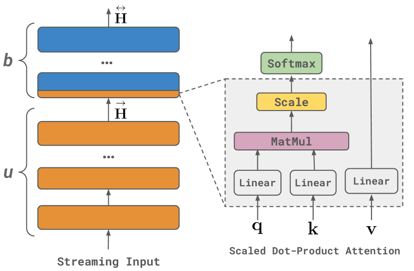
Figure 1: In Hybrid encoder architecture, the earlier $u$ layers are unidirectional, and later $b$ layers are bidirectional. The blue layers require restart, i.e. at each timestep when the model receives a new token of the streaming input, these layers will recompute all intermediate representations for all the input tokens. The orange layers (like unidirectional layers) can avoid restart by caching the intermediate state. A portion of the first bidirectional layer before application of softmax also does not require restart and can be cached.

The Hybrid encoder is a combination of unidirectional and bidirectional encoding layers, where the early layers are unidirectional and the later layers are bidirectional as shown in Figure 2. The earlier unidirectional layers do not require a restart as the previous tokens’ embeddings do not need to be updated for the newly received tokens. Thus, the Hybrid encoder only require a restart for its later bidirectional layers. Formally, the Hybrid encoder has $u$ unidirectional and $b$ bidirectional layers where total layers in the model are $u+b=l$. Let $\overset{\text{$\rightarrow$}}{L}$ and $\overset{\text{$\leftrightarrow$}}{L}$ denote unidirectional and bidirectional layers in the model respectively. Each of the $\overset{\text{$\rightarrow$}}{L}$ layers are one of the existing unidirectional layers - RNN, GRU, transformer with causal masking etc. with the first of these being the static embedding layer. Each of the $\overset{\text{$\leftrightarrow$}}{L}$ layers are bidirectional layers, being one of bi-GRU, bi-LSTM, transformer etc.

Notation	Meaning
$\overset{\text{$\rightarrow$}}{L}$, $\overset{\text{$\leftrightarrow$}}{L}$	Unidirectional and bidirectional layers, respectively.
$\overset{\text{$\rightarrow$}}{\textbf{h}}_{i}$, $\overset{\text{$\leftrightarrow$}}{\textbf{h}}_{i,t}$	Encoding of $x_{i}$ token when $t$ tokens have been received, using $\overset{\text{$\rightarrow$}}{L}$ and $\overset{\text{$\rightarrow$}}{L}+\overset{\text{$\leftrightarrow$}}{L}$, respectively.
$\overset{\text{$\rightarrow$}}{\textbf{H}}_{t}$, $\overset{\text{$\leftrightarrow$}}{\textbf{H}}_{t}$	$\overset{\text{$\rightarrow$}}{\textbf{h}}_{i}$, $\overset{\text{$\leftrightarrow$}}{\textbf{h}}_{i,t}$ of first $t$ tokens, respectively.
$\overset{\text{$\rightarrow$}}{y}_{i}$, $\overset{\text{$\leftrightarrow$}}{y}_{i,t}$	Predicted label of $x_{i}$ token using $\overset{\text{$\rightarrow$}}{\textbf{h}}_{i}$ and $\overset{\text{$\leftrightarrow$}}{\textbf{h}}_{i,t}$, respectively.

Table 2: Notations used in Hybrid encoder for layers, token representations, and predicted labels.

3.1.1 Hybrid Encoder in Offline Setting:

First, the input tokens $\mathbf{x}$ are fed to $u$ unidirectional layers to get the unidirectional encodings $\overset{\text{$\rightarrow$}}{\mathbf{H}}$,

$$\overset{\text{$\rightarrow$}}{\mathbf{H}}=[\overset{\text{$\rightarrow$}}{\mathbf{h}}_{1},\cdots\overset{\text{$\rightarrow$}}{\mathbf{h}}_{n}]=\overbrace{\overset{\text{$\rightarrow$}}{L}\circ\overset{\text{$\rightarrow$}}{L}\circ\cdots\overset{\text{$\rightarrow$}}{L}}^{u\text{ layers}}(\mathbf{x})$$ (1)

where $\circ$ denotes the functional composition and $\overset{\text{$\rightarrow$}}{\mathbf{h}}_{i}$ is the unidirectional encoding for the token $x_{i}$. Then the bidirectional encodings $\overset{\text{$\leftrightarrow$}}{\mathbf{H}}$ are computed and used to predict the label sequence:

$$\overset{\text{$\leftrightarrow$}}{\mathbf{H}}=[\overset{\text{$\leftrightarrow$}}{\mathbf{h}}_{1},\cdots\overset{\text{$\leftrightarrow$}}{\mathbf{h}}_{n}]=\overbrace{\overset{\text{$\leftrightarrow$}}{L}\circ\overset{\text{$\leftrightarrow$}}{L}\circ\cdots\overset{\text{$\leftrightarrow$}}{L}}^{b\text{ layers}}({\overset{\text{$\rightarrow$}}{\mathbf{H}}})$$ (2)

The final offline labels are obtained by passing $\overset{\text{$\leftrightarrow$}}{\mathbf{H}}$ through a feed-forward neural network layer.

3.1.2 Hybrid Encoder in Streaming Setting

In the streaming setting, the unidirectional layers’ computation can be cached. These cached intermediate representations for the previously received tokens $\mathbf{x}_{t-1}$ are used in computing the unidirectional encoding $\overset{\text{$\rightarrow$}}{\mathbf{h}}_{t}$ of the new token $x_{t}$. This along with the cached unidirectional encoding of $\mathbf{x}_{t-1}$ gives us $\overset{\text{$\rightarrow$}}{\mathbf{H}}_{t}=[\overset{\text{$\rightarrow$}}{\mathbf{H}}_{t-1};\overset{\text{$\rightarrow$}}{\mathbf{h}}_{t}]$. The bidirectional encoding, however, for each token in $\mathbf{x}_{t}$ is restarted at time t as $\overset{\text{$\leftrightarrow$}}{\mathbf{H}}_{t}=[\overset{\text{$\leftrightarrow$}}{\mathbf{h}}_{1,t},\cdots\overset{\text{$\leftrightarrow$}}{\mathbf{h}}_{t,t}]$ using the obtained final unidirectional encoding $\overset{\text{$\rightarrow$}}{\mathbf{H}}_{t}$ as input.

3.1.3 Training and Inference of Hybrid Encoder

We predict labels over both $\overset{\text{$\rightarrow$}}{\mathbf{H}}_{t}$ and $\overset{\text{$\leftrightarrow$}}{\mathbf{H}}_{t}$ of the Hybrid encoder using a linear layer with softmax at each timestep. Let $\overset{\text{$\leftrightarrow$}}{\mathbf{y}}_{t}=[\overset{\text{$\leftrightarrow$}}{y}_{1,t},\cdots\overset{\text{$\leftrightarrow$}}{y}_{t,t}]$ denote the predictions over bidirectional embeddings at time $t$ for all the tokens received so far. Let $\overset{\text{$\rightarrow$}}{\mathbf{y}}_{t}=[\overset{\text{$\rightarrow$}}{y}_{1},\cdots\overset{\text{$\rightarrow$}}{y}_{t}]$ be predictions over unidirectional embeddings at time $t$. While the unidirectional predictions do not perform as well as bidirectional predictions, these auxiliary predictions enables waited restarts (§3.2).

Hybrid encoder is trained over the offline input-output sequence pairs and optimize both the bidirectional predictions and unidirectional predictions. for the standard softmax cross entropy loss against the offline ground truth label sequence $\mathbf{y}^{*}$. In order to preserve the strong performance of the BiDi encoders, we inhibit backward flow of gradient from the parameters $\theta_{uni}$ of unidirectional prediction head (consisting only of a linear layer with softmax) to the remaining parameters - $\theta_{bi}$.Following are the losses of these two portions of the model, optimized together with equal weight.

$$\mathcal{L}(\theta_{bi},\overset{\text{$\leftrightarrow$}}{\mathbf{y}}_{n},\mathbf{y}^{*}) =CE(\overset{\text{$\leftrightarrow$}}{\mathbf{y}}_{t},\mathbf{y}^{*})$$ (3)

$$\mathcal{L}(\theta_{uni},\overset{\text{$\rightarrow$}}{\mathbf{y}}_{n},\mathbf{y}^{*}) =CE(\overset{\text{$\rightarrow$}}{\mathbf{y}}_{t},\mathbf{y}^{*})$$ (4)

$$\mathcal{L}(\theta)=\mathcal{L}(\theta_{bi},\overset{\text{$\leftrightarrow$}}{\mathbf{y}}_{n},\mathbf{y}^{*}) +\mathcal{L}(\theta_{uni},\overset{\text{$\rightarrow$}}{\mathbf{y}}_{n},\mathbf{y}^{*})$$ (5)

3.2 Waited Restarts

The Hybrid encoder reduces the computational overhead of each restart by limiting the recomputation over previous tokens only to the later bidirectional layers. However, restarting at each step is not required and the auxiliary predictions from the unidirectional layers can suffice.

We define a variable $\textsc{restart}(t)$ to decide whether to restart the bidirectional layers at time $t$. When $\textsc{restart}(t)=1$, we restart the model to get the bidirectional predictions $\overset{\text{$\leftrightarrow$}}{\mathbf{y}}_{t}$ as the final predicted label sequence $\hat{\mathbf{y}}_{t}=\overset{\text{$\leftrightarrow$}}{\mathbf{y}_{t}}$. If $\textsc{restart}(t)=0$, the model does not run the bidirectional encoder, but uses the unidirectional encoding to predict the current token’s label $\overset{\text{$\rightarrow$}}{y}_{t}$ and copy the label sequence from the previous step $\hat{\mathbf{y}}_{t-1}$ to obtain $\hat{\mathbf{y}}_{t}$. Formally, the predicted sequence $\hat{\mathbf{y}}_{t}=(\hat{y}_{1,t},\cdots\hat{y}_{t,t})$ at time $t$ is

$$\hat{\mathbf{y}}_{t}=\begin{cases}~{}\overset{\text{$\leftrightarrow$}}{\mathbf{y}}_{t}&\text{if }\textsc{restart}(t)=1\text{ or }t=n\\ ~{}[\hat{\mathbf{y}}_{t-1};\overset{\text{$\rightarrow$}}{y}_{t}]&\text{otherwise}\end{cases}$$ (6)

where ‘;’ denotes the concatenation. We always restart in the final timestep (i.e., $\textsc{restart}(n)=1$) to preserve the offline performance.

3.2.1 Adaptive Restart Module (ARM)

A baseline restart strategy for waited restarts would be to restart the bidirectional layers every fixed $k$ steps, i.e., $\textsc{restart}(t)=1$ whenever $t$ is a multiple of $k$. Note that $k=1$ reduces to a Hybrid encoder model without waited restarts. We refer to this as Restart-$k$.

Rather than having a heuristic function for $\textsc{restart}(t)$, we can let a lightweight parametric module determine when to do the restart by determining ${\textsc{restart}}_{\theta}{(t)}$ for each $t$. We refer to this as Adaptive Restart Module (ARM). We first discuss the set of features for ARM (§3.2.2), followed by its architecture (§3.2.3) and training (§3.2.4).

3.2.2 Input Features for ARM

We use Hybrid encoder’s intermediate representations that do not require restart as the features for ARM. This includes the unidirectional layers as well as from the pre-softmax features from the first $\overset{\text{$\leftrightarrow$}}{L}$ layer. The main motivation to use these features is to incorporate more information without incurring any restarts.

The following features are stored in unidirectional cache and used without any restart for ARM:

1. unidirectional encodings $\overset{\text{$\rightarrow$}}{\mathbf{h}}_{t}$ from the last unidirectional layer computed once and cached for capturing the backward flow,

2. query $\mathbf{q}_{t}$ and key $\mathbf{k}_{t}$ from the first bidirectional layer computed only from $\overset{\text{$\rightarrow$}}{\mathbf{h}}_{t}$,

3. unnormalized forward attention scores $\mathbf{a}_{t}=[\mathbf{q}_{1}\cdot\mathbf{k}_{t},\cdots,\mathbf{q}_{t-1}\cdot\mathbf{k}_{t}]$ from the first bidirectional layer, where ‘$\cdot$’ is the dot product. These scores are concatenated across the prefix tokens (restricted and padded to latest $m$ tokens) across all heads.

These features are then concatenated and provided as input to the ARM as $\mathbf{f}_{t}=[\overset{\text{$\rightarrow$}}{\mathbf{h}}_{t},\mathbf{q}_{t},\mathbf{k}_{t},\mathbf{a}_{t}]$.

3.2.3 ARM Architecture

We use a single-layered Gru Cho et al. (2014) to predict restart. The probability of restart $p_{\theta}(\textsc{restart}(t)=1)$ is modeled as,

$$(\mathbf{o}_{t},\mathbf{s}_{t}) =\text{{Gru}}(\mathbf{f}_{t},\mathbf{s}_{t-1})$$ (7)

$$p_{\theta}(\textsc{restart}(t)=1) =\sigma(\textsc{Linear}(\mathbf{o}_{t}))$$ (8)

Here $\mathbf{s}_{t}$ and $\mathbf{o}_{t}$ are the GRU hidden state and output at time $t$, respectively. These outputs can be post-processed to handle too frequent or too infrequent waiting and obtain the final selector predictions.Details can be found in Appendix (§A.2).

3.2.4 Training the ARM

Ideally, Hybrid encoder should restart only when it would lead to improved predictions over the prefixes i.e., more number of prefix inputs should have the same output as the the offline ground truth for those prefixes. We use this to define our ground truth restart sequence for training the ARM.

Given the ground truth offline tag sequence $\mathbf{y}^{*}$, unidirectional predictions $\overset{\text{$\rightarrow$}}{\mathbf{y}}=[\overset{\text{$\rightarrow$}}{y}_{1},\cdots\overset{\text{$\rightarrow$}}{y}_{n}]$ and final bidirectional prediction sequence over each of the $n$ prefixes $\overset{\text{$\leftrightarrow$}}{\mathbf{Y}}=[\overset{\text{$\leftrightarrow$}}{\mathbf{y}}_{1},\cdots\overset{\text{$\leftrightarrow$}}{\mathbf{y}}_{n}]$, we define the ground truth policy $\textsc{Restart}^{*}(t)=\pi^{*}_{t}$ for ARM, at time $t$, as follows.

$$\pi^{*}_{t}=\begin{cases}1&\text{if }|y^{*}_{\leq t}=\overset{\text{$\rightarrow$}}{y}_{\leq t}|<|y^{*}_{\leq t}=\overset{\text{$\leftrightarrow$}}{y}_{\leq t}|\\ 0&\text{otherwise}\end{cases}$$ (9)

The policy decides to restart at time $t$ if more tokens in bidirectional predictions match with the ground truth ($|y^{*}_{\leq t}=\overset{\text{$\leftrightarrow$}}{y}_{\leq t}|$) than those from unidirectional predictions ($|y^{*}_{\leq t}=\overset{\text{$\rightarrow$}}{y}_{\leq t}|$). ARM is trained against this policy with features from a frozen and trained Hybrid encoder model with a standard binary cross entropy loss.

Current Token	Prefix Predictions	Total	Unnecessary	Exact Match	Exact Match
		Edits	Edits	w/ ground truth	w/ final prediction
find	O	1	0	1	1
new	O O	2	1	1	1
york	O LOC LOC	4	3	2	1
times	O ORG ORG ORG	7	3	2	2
square	O ORG ORG ORG LOC	8	3	2	3
Ground Truth	O LOC LOC LOC LOC	EO=$\frac{\text{Unnecessary ~{}Edits}}{\text{Total ~{}Edits}}=\frac{3}{8}$    Streaming EM = $\frac{\text{EM w/ ground truth}}{\text{\# steps}}=\frac{2}{5}$    RC = $\frac{\text{EM w/ final labels}}{\text{\# steps}}=\frac{3}{5}$

Table 3: Example computation for the metrics described in §4.1 . EO is calculated as fraction of edits that were unnecessary. RC measures the fraction of prefix predictions that matches the model’s final predictions. Streaming EM measures the fraction of prefix predictions that are correct with respect to the ground truth labels.

4 Experimental Setup

Datasets and Tasks.

We consider four common sequence tagging tasks – Slot Filling over SNIPS Coucke et al. (2018), Semantic Role Labelling (SRL) over Ontonotes Pradhan et al. (2013), and Named Entity Recognition (NER) and Chunking (CHUNK) over CoNLL-2003 Sang and Meulder (2003). The standard train, dev and test splits are used for all datasets.

Models and Baselines.

For our models, we consider a layer budget of 4 for the encoder. Naturally, our baselines are the UniDi encoder and BiDi encoder with all unidirectional and bidirectional layers, respectively. For HEAR, we tune for the optimal fractions of unidirectional layers in encoder by selecting the one that maximizes the offline F1 performance over the development set. We consider Restart-$k$ baseline for ARM. For each dataset, we picked the best value of $k$ from $\{2,3,5,8\}$, maximizing the Streaming EM over development set.

4.1 Metrics

The model evaluation is done over three criteria: offline performance over complete input text, streaming performance over prefixes and efficiency of running the model in streaming settings.

Offline Metrics.

The offline performance of the model is measured using the widely used chunk-level F1 score for sequence labelling tasks Sang and Meulder (2003).

GFLOPs.

We measure total number of Floating Point Operations (FLOPs) required for running the model in a streaming setting in GigaFLOPs (GFLOP), estimated via XLA compiler’s High Level Operations (HLO) Sabne (2020). GFLOP positively correlates with how computation-heavy a model is and its wall-clock execution time.

Streaming Metrics.

An ideal streaming model should predict the correct labels for all prefixes early Trinh et al. (2018) and avoid unnecessary label flips. Following previous works Madureira and Schlangen (2020); Kahardipraja et al. (2021), we use Edit Overhead (EO) and Relative Correctness (RC) metrics from Baumann et al. (2011).

EO (Edit Overhead) is a measure of the fraction of the label edits that were unnecessary with respect to the final prediction on complete output. Consider the example in Table 3. At the first timestep, the token “find” is assigned a label “O” from “N/A”; taking the total edits to $1$. Similarly, in the second timestep, the newly received token “new” gets a label edit; taking the total edit to $2$. In the third timestep, however, not only the newly received token “york” receives a label edit but the second token “new” is also edited from “O” to “LOC”; resulting in $4$ total edits. Of these edits, the label edit for token "new" in timestep 2 from “N/A” to “O” was unnecessary as it differs from its final label “ORG”. Similarly, the label flips for “new” and “york” in the timestep 3 from “O” and “N/A” to “LOC” and “LOC”, respectively, were also unnecessary. Cumulatively, towards the end of fifth timestep, we have $3$ out of $8$ total edits which were overhead. Thus, the EO turns out to be $\frac{3}{8}$, where lower is better.

RC measures the relative correctness of prefixes, i.e. correctness of prefix prediction sequence with respect to the final label set over the complete input. For the example in Table 3, only the label sequence in the first timestep (“O”), fourth timestep (“O ORG ORG ORG”) and final (fifth) timestep are prefixes of the label sequence in the final timestep (“O ORG ORG ORG LOC”). Thus $3$ prefixes of a total $5$ prefixes were correct. So, the Relative Correctness is $\frac{3}{5}$, where higher is better.

While EO and RC capture consistency and stability in streaming predictions, neither of these measures performance with respect to the ground truth label over offline input. Relying on these metrics alone is not sufficient to measure streaming performance. For example, a UniDi encoder achieves perfect EO and RC scores, despite have poor predictions with respect to the offline ground truth. Thus, we consider Streaming Exact Match (Streaming EM), which is the streaming setting analogue of the Exact Match metric. Streaming EM calculates the percentages of prefix label sequence which are correct with respect to the offline ground truth labels. For example in Table 3, only the first label sequence (“O”) for input “find” and third label sequence (“O LOC LOC”) for input “find new york” is a prefix of the ground truth label sequence (“O LOC LOC LOC LOC”), leading to only $2$ out of $5$ prefix label sequence being correct. Thus, the Streaming EM is $\frac{2}{5}$. Similar to RC, higher score is better as more prefixes have exact matches.

Model	SNIPS	CHUNK	NER	SRL
UniDi encoder	86.8	88.1	73.8	56.4
Hybrid encoder	93.0	89.4	86.8	80.0
BiDi encoder	93.1	89.4	86.0	80.1

Table 4: Offline F1 over test set of datasets described in §4. On all datasets, Hybrid encoder achieves performance parity with the BiDi models.

Dataset	GFLOP $\downarrow$			Streaming EM $\uparrow$			EO $\downarrow$			RC $\uparrow$
	BiDi	Hybrid	HEAR	BiDi	Hybrid	HEAR	BiDi	Hybrid	HEAR	BiDi	Hybrid	HEAR
SNIPS	74.7	43.4	21.6	75.1	72.5	85.1	15.9	16.7	6.3	78.2	76.3	88.5
CHUNK	238.8	126.3	91.3	77.7	77.7	77.9	5.0	4.8	4.5	91.6	91.9	91.6
NER	238.8	126.2	83.8	79.3	78.2	81.9	8.7	8.3	5.4	87.2	88.2	90.9
SRL	741.2	557.7	460.4	43.6	49.1	50.6	33.0	29.9	21.0	56.0	61.5	62.5

Table 5: Streaming performance over test set of datasets. HEAR significantly outperforms BiDi on all metrics improving upon efficiency and performance. Direction of arrow indicates whether higher or lower is better.

5 Experimental Results

In this section, we provide empirical results to answer the following questions:

1. In offline setting, does Hybrid encoder achieve parity with BiDi encoders?

2. In streaming setting, by how much does Hybrid encoder reduce GFLOPs count?

3. Does HEAR improve streaming performance and save on GFLOP count?

Hybrid Encoder’s Offline Performance is Competitive to BiDi Encoders.

Table 4 shows the offline F1 scores of the Hybrid encoder, UniDi and BiDi encoders across the four tasks. The Hybrid encoder has similar offline F1 as BiDi encoders. In fact, on NER, it even outperforms it by a margin of 0.8 F1 score. As expected, the UniDi model performs poorly compared to the BiDi encoder across all the tasks. From here on, we omit UniDi encoder.

Hybrid Encoder Improves Streaming Efficiency.

Table 5 shows the GFLOP (per input instance) in streaming settings across the four datasets for the Hybrid encoder and BiDi encoders, with a trivial restart at every new token to get predictions over streaming text. We observe that Hybrid encoder consistently offers lower GFLOP count than BiDi encoder across the datasets, and in three of the four datasets, offering more than 40% FLOP reduction. However, Hybrid encoder does not improve on streaming performance (Streaming EM, EO, and RC) over BiDi, and its FLOP can be further reduced. We next see how incorporating HEAR addresses this.

HEAR Improves Streaming Efficiency and Performance.

Across all datasets, we observe HEAR further reduces GFLOP count from the already computationally lighter Hybrid encoder, giving us upto 71% total FLOP reduction from BiDi. HEAR has better streaming predictions, as its Streaming EM is much higher (upto +10.0) than BiDi, improving on the shortcoming of Hybrid. This highlights that naively restarting at each timestep can worsen the streaming performance, as evident through the lower performance of Hybrid and BiDi. HEAR also offers reduced number of avoidable label flips, as signified by a lower EO. Its high RC score signifies that its streaming predictions are more consistent with its final prediction.

All these results demonstrate that HEAR preserves the offline performance of BiDi encoders, while being computationally lighter by 58.9% on average across tasks. HEAR has more consistent streaming predictions which are accurate with respect to offline ground truth.

6 Analysis and Ablations

Dataset	Offline F1$\uparrow$		Streaming EM $\uparrow$		EO $\downarrow$		ARM Classification
	BiDi	UniDi	restart-$k$	ARM	restart-$k$	ARM	Micro-F1
SNIPS	93.6	79.1	82.1	85.3	7.9	6.0	79.5
CHUNK	90.4	86.8	75.6	76.5	4.5	4.5	67.1
NER	91.3	77.9	85.6	87.8	4.1	4.0	75.7
SRL	79.7	42.8	41.8	48.9	31.5	21.6	80.2

Table 6: Development set ablation and analyses. From left to right - comparing performance of Hybrid encoder over sequence tagging using its bidirectional (final) vs unidirectional (intermediate) encoding, comparison of Streaming EM and EO of restart-k vs ARM, and the performance of ARM w.r.t. its ground truth policy labels.

In this section, we perform various analysis pertaining to the Hybrid encoder and ARM.

6.1 Hybrid Encoder’s Unidirectional Layers Performance

Table 6 compares the performance of the prediction over the intermediate (unidirectional) and final (bidirectional) encodings for the best HEAR model. While the intermediate ones lag in comparison to the final, we get decent performance from intermediate ones across all except for SRL dataset. This shows that, when used selectively, UniDi intermediate predictions can serve as a good source of auxiliary predictions.

6.2 ARM vs Restart-$k$.

Table 6 shows the performance of baseline - the best Restart-$k$ from {2, 3, 5, 8} over dev set Streaming EM and the ARM. We observe that across all the datasets, on both Streaming EM and EO metric, ARM performs significantly better than the heuristic Restart-$k$ mechanism. This shows that using a fixed length wait is not sufficient.

6.3 Intrinsic Performance of ARM

Table 6 shows the performance of the ARM on its binary classification task. Given the lightweight ARM architecture and the task complexity, the performance is satisfactory with 80.2 $F_{1}$. However, there is a considerable margin for its improvement both in terms of model architecture and features.

6.4 ARM’s Architecture Ablation

Dataset	Streaming EM $\uparrow$	EO $\downarrow$
No ARM	73.8	16.3
Linear ARM	81.3	6.8
MLP ARM	81.4	6.9
GRU ARM	85.3	6.0

Table 7: Performance of HEAR with different ARM model architectures over SNIPS development set.

Table 7 shows the Streaming EM and EO scores of HEAR with different ARM model architectures for the SNIPS development set. We observe that HEAR having either a Linear layer or MLP as ARM does much better than having no ARM and restarting at each timestep. However, modeling ARM as a GRU recurrent model gives the best scores in both metrics.

7 Related Work

Streaming (or incremental) setting has been widely studied in machine translation and parsing, dating as far back as two decades Larchevêque (1995); Lane and Henderson (2001). Specifically, for incremental parsing, there are two broad approaches that have been studied: transition-based and graph-based. Transition-based incremental parsers allow for limited backtracking and correcting parsing over prefixes by keeping track of multiple parse segments Buckman et al. (2016) or via beams search Bhargava and Penn (2020). Such methods can fail on garden-path sentences and long-range dependencies and only work proficiently with a large beam. Graph-based parsers incrementally assign scores to edges of the graph, discarding those edges that cause conflicts to tree-structure of the graph. Yang and Deng (2020) proposed an attach-juxtapose system to grow the tree, requiring restart at each new token over streaming input. Kitaev et al. (2022) improved on its efficiency by proposing a information bottleneck. However, these methods rely on the structured nature of parsing output can not be adapted to incremental sequence tagging tasks without restarting at each token.

Recently,  Madureira and Schlangen (2020) benchmarked the modern encoders on streaming sequence labelling and observed poor streaming performance of pretrained transformer models. They explored improvement strategies by adopting techniques from other streaming streaming like chunked training  Dalvi et al. (2018), truncated training  Köhn (2018) (training model on heuristically-aligned partial input-output pairs), and prophecy Alinejad et al. (2018) (autocompleting input using a separate language model). They observed performance degradation from truncated training unless used with prophecies. However, running a language model at each timestep for prophecy is computationally infeasible. Therefore, unlike our approach, neither methods can improve performance feasibly.

Previous works have attempted to improve computation efficiency in BiDi encoders. Monotonic attention moves away from $O(n^{2})$ soft attention overhead by restricting attention to monotonically increase across timesteps Raffel et al. (2017); Chiu and Raffel (2018); Ma et al. (2020). However, unlike HEAR, such attempts can’t maintain offline performance. Recently, Kahardipraja et al. (2021) used linear transformer  Katharopoulos et al. (2020) as unidirectional model using masking for streaming sequence tagging and classification. This approach performs well under the assumption of delayed output  Grissom II et al. (2014); Oda et al. (2015), a relaxation, where the model waits for additional tokens before predicting. Furthermore, the unidirectional model could not revise its output, rendering the model incapable of handling long-range dependency or tasks that go backward like SRL — an ability common to any model with some bidirectionality, such as HEAR. Similar drawbacks were in the partial bidirectional encoder, a bidirectional attention with restricted window, proposed by Iranzo Sanchez et al. (2022).

Improving efficiency through adaptive computing has been independently studied for reasoning-based tasks  Eyzaguirre and Soto (2020), text generation models  Arumae and Bhatia (2020); Eyzaguirre et al. (2022) and diffusion models  Ye et al. (2022). These works are restricted to offline settings and can be readily incorporated within the proposed overall approach of HEAR.

8 Conclusion

We propose HEAR for sequence tagging in streaming setting where the input is received one token at a time to the model. The encoder in our model is Hybrid encoder where early layers are unidirectional and later are bidirectional. It reduces the computational cost in streaming settings, by reducing the need of restart only to the later bidirectional layers while preserving the offline performance of the model. HEAR additionally consists of an ARM to predict when to restart the model. Using ARM leads to reduced number of restart of the encoder, leading to better streaming performance and further savings in computation. Compared to BiDi encoders, our model, HEAR (Hybrid encoder + ARM) reduces the computation by upto 71% in streaming settings while maintaining the performance of the BiDi encoders across various sequence tagging tasks. HEAR improved streaming EM by upto +10.0% and reduced unnecessary edits by upto -12.0%.

Limitations

An additional but small training cycle is required to train the lightweight ARM module of HEAR in order to reap the benefits of extra savings in efficiency and streaming performance. Also, even though we do not assume any language specific-design choices, we benchmarked on the standard streaming sequence labelling benchmark datasets, all of which were in English.

Appendix A Experiment Details

A.1 Implementation Details

All the experiments were done using the Flax Heek et al. (2020) and Jax Bradbury et al. (2018) with Adam optimizer Kingma and Ba (2014) on TPUs. We measure flops in terms of XLA’s HLO Sabne (2020). The optimizer’s learning rate is set to 1e-3, betas are set to default at (0.9, 0.999), batch size is 256 and feedforward hiden is 2048 with 512 transformer dimension and 8 heads.

For all the datasets we use the standard splits, the links to which can be found in their respective papers along with statistics. Following Ratinov and Roth (2009), we use the BIOES tagging scheme for the NER task and BIO scheme for the rest. In SRL, following He et al. (2017) the indicator for predicate verb is also used as input the along with the sentence.

All the values over test sets are averaged across four seeds. For experiments involving ARM we average across four different Hybrid encoder trained from different seeded initialization. We initialize static embeddings with 300 dimensional glove embedding Pennington et al. (2014).

A.2 Postprocessing ARM Predictions

We post process the ARM predictions to prevent too frequent or too infrequent restarts. Specifically, for hyperparameters $\alpha$ and $\beta$ where $0\leq\alpha<\beta$, at any time $t$, if the ARM hasn’t restarted once since $max(0,t-\beta)$ timesteps, then ARM’s prediction is set to 1, else, if the ARM has restarted atleast once since $max(0,t-\alpha)$ timesteps, then it is set to 0. We tune for the values of $\alpha$ and $\beta$ in the range {0, 1, 2, 3, 5, 10} over the development set.

We also observe that even if bidirectional layers improve predictions over previous tokens, for the latest token only, the unidirectional label $\overset{\text{$\rightarrow$}}{y}_{t}$ is often better than $\overset{\text{$\leftrightarrow$}}{y}_{t}$. If this is observed, then, we exclude the most recent token from getting updated during restart. We tune for this binary postprocessor over the development set as well.

Appendix B Analysis and Ablation

B.1 Benefits of Optimizing Unidirectional Predictor Separately

In Hybrid encoder the performance we inhibit backward gradient flow from the auxiliary predictor over the unidirectional layers unidirectional. This is because we observed offline F1 performance drop of bidirectional predictor when trained with unidirectional predictor, dropping from 81.20 to 71.62 on CoNLL development set. Even after tuning for loss scaling for the to predictors in ratio {1:1, 3.3:1, 10:1, 33:1, 100:1}, the performance was only increased upto 75.06 F1.

B.2 Oracle Policy for ARM

We also experimented with alternate policy for ARM where it’s label is conditioned on the last bidirectional restart. However, it led to a performance drop in terms of Streaming EM from 86.7 to 83.0, as observed across SNIPS development set. We attribute this poor performance on alternate policy, due to the lightweight nature of ARM. Thus, we did not proceed with this policy.

References

- Alinejad et al. (2018) Ashkan Alinejad, Maryam Siahbani, and Anoop Sarkar. 2018. Prediction improves simultaneous neural machine translation. In Proceedings of the 2018 Conference on Empirical Methods in Natural Language Processing, pages 3022–3027, Brussels, Belgium. Association for Computational Linguistics.
- Arumae and Bhatia (2020) Kristjan Arumae and Parminder Bhatia. 2020. Calm: Continuous adaptive learning for language modeling.
- Baumann et al. (2011) Timo Baumann, Okko Buß, and David Schlangen. 2011. Evaluation and optimisation of incremental processors. In Dialogue and Discourse, 2011.
- Bhargava and Penn (2020) Aditya Bhargava and Gerald Penn. 2020. Supertagging with CCG primitives. In Proceedings of the 5th Workshop on Representation Learning for NLP, pages 194–204, Online. Association for Computational Linguistics.
- Bradbury et al. (2018) James Bradbury, Roy Frostig, Peter Hawkins, Matthew James Johnson, Chris Leary, Dougal Maclaurin, George Necula, Adam Paszke, Jake VanderPlas, Skye Wanderman-Milne, and Qiao Zhang. 2018. JAX: composable transformations of Python+NumPy programs.
- Buckman et al. (2016) Jacob Buckman, Miguel Ballesteros, and Chris Dyer. 2016. Transition-based dependency parsing with heuristic backtracking. In Proceedings of the 2016 Conference on Empirical Methods in Natural Language Processing, pages 2313–2318, Austin, Texas. Association for Computational Linguistics.
- Cai and de Rijke (2016) Fei Cai and Maarten de Rijke. 2016. A survey of query auto completion in information retrieval. Found. Trends Inf. Retr., 10(4):273–363.
- Chang et al. (2022) Shuo-yiin Chang, Guru Prakash, Zelin Wu, Qiao Liang, Tara N. Sainath, Bo Li, Adam Stambler, Shyam Upadhyay, Manaal Faruqui, and Trevor Strohman. 2022. Streaming Intended Query Detection using E2E Modeling for Continued Conversation.
- Chiu and Raffel (2018) Chung-Cheng Chiu and Colin Raffel. 2018. Monotonic chunkwise attention. In International Conference on Learning Representations.
- Cho and Esipova (2016) Kyunghyun Cho and Masha Esipova. 2016. Can neural machine translation do simultaneous translation?
- Cho et al. (2014) Kyunghyun Cho, Bart van Merrienboer, Caglar Gulcehre, Dzmitry Bahdanau, Fethi Bougares, Holger Schwenk, and Yoshua Bengio. 2014. Learning Phrase Representations using RNN Encoder-Decoder for Statistical Machine Translation.
- Coucke et al. (2018) Alice Coucke, Alaa Saade, Adrien Ball, Théodore Bluche, Alexandre Caulier, David Leroy, Clément Doumouro, Thibault Gisselbrecht, Francesco Caltagirone, Thibaut Lavril, Maël Primet, and Joseph Dureau. 2018. Snips Voice Platform: an Embedded Spoken Language Understanding system for private-by-design voice interfaces.
- Dalvi et al. (2018) Fahim Dalvi, Nadir Durrani, Hassan Sajjad, and Stephan Vogel. 2018. Incremental decoding and training methods for simultaneous translation in neural machine translation. In Proceedings of the 2018 Conference of the North American Chapter of the Association for Computational Linguistics: Human Language Technologies, Volume 2 (Short Papers), pages 493–499, New Orleans, Louisiana. Association for Computational Linguistics.
- Devlin et al. (2019) Jacob Devlin, Ming-Wei Chang, Kenton Lee, and Kristina Toutanova. 2019. BERT: Pre-training of Deep Bidirectional Transformers for Language Understanding. In Proceedings of the 2019 Conference of the North American Chapter of the Association for Computational Linguistics: Human Language Technologies, Volume 1 (Long and Short Papers), Minneapolis, Minnesota. Association for Computational Linguistics.
- Eyzaguirre et al. (2022) Cristobal Eyzaguirre, Felipe del Rio, Vladimir Araujo, and Alvaro Soto. 2022. DACT-BERT: Differentiable adaptive computation time for an efficient BERT inference. In Proceedings of NLP Power! The First Workshop on Efficient Benchmarking in NLP, pages 93–99, Dublin, Ireland. Association for Computational Linguistics.
- Eyzaguirre and Soto (2020) Cristóbal Eyzaguirre and Álvaro Soto. 2020. Differentiable adaptive computation time for visual reasoning. In 2020 IEEE/CVF Conference on Computer Vision and Pattern Recognition (CVPR), pages 12814–12822.
- Grissom II et al. (2014) Alvin Grissom II, He He, Jordan Boyd-Graber, John Morgan, and Hal Daumé III. 2014. Don’t until the final verb wait: Reinforcement learning for simultaneous machine translation. In Proceedings of the 2014 Conference on Empirical Methods in Natural Language Processing (EMNLP), pages 1342–1352, Doha, Qatar. Association for Computational Linguistics.
- Gu et al. (2017) Jiatao Gu, Graham Neubig, Kyunghyun Cho, and Victor O.K. Li. 2017. Learning to Translate in Real-time with Neural Machine Translation. In Proceedings of the 15th Conference of the European Chapter of the Association for Computational Linguistics: Volume 1, Long Papers, pages 1053–1062, Valencia, Spain. Association for Computational Linguistics.
- He et al. (2017) Luheng He, Kenton Lee, Mike Lewis, and Luke Zettlemoyer. 2017. Deep Semantic Role Labeling: What Works and What’s Next. In Proceedings of the 55th Annual Meeting of the Association for Computational Linguistics (Volume 1: Long Papers), pages 473–483, Vancouver, Canada. Association for Computational Linguistics.
- Heek et al. (2020) Jonathan Heek, Anselm Levskaya, Avital Oliver, Marvin Ritter, Bertrand Rondepierre, Andreas Steiner, and Marc van Zee. 2020. Flax: A neural network library and ecosystem for JAX.
- Iranzo Sanchez et al. (2022) Javier Iranzo Sanchez, Jorge Civera, and Alfons Juan-Císcar. 2022. From simultaneous to streaming machine translation by leveraging streaming history. In Proceedings of the 60th Annual Meeting of the Association for Computational Linguistics (Volume 1: Long Papers), pages 6972–6985, Dublin, Ireland. Association for Computational Linguistics.
- Kahardipraja et al. (2021) Patrick Kahardipraja, Brielen Madureira, and David Schlangen. 2021. Towards Incremental Transformers: An Empirical Analysis of Transformer Models for Incremental NLU. In Proceedings of the 2021 Conference on Empirical Methods in Natural Language Processing, pages 1178–1189, Online and Punta Cana, Dominican Republic. Association for Computational Linguistics.
- Katharopoulos et al. (2020) Angelos Katharopoulos, Apoorv Vyas, Nikolaos Pappas, and François Fleuret. 2020. Transformers are RNNs: Fast autoregressive transformers with linear attention. In Proceedings of the 37th International Conference on Machine Learning, volume 119 of Proceedings of Machine Learning Research, pages 5156–5165. PMLR.
- Kingma and Ba (2014) Diederik P. Kingma and Jimmy Ba. 2014. Adam: A Method for Stochastic Optimization.
- Kitaev et al. (2022) Nikita Kitaev, Thomas Lu, and Dan Klein. 2022. Learned incremental representations for parsing. In Proceedings of the 60th Annual Meeting of the Association for Computational Linguistics (Volume 1: Long Papers), pages 3086–3095, Dublin, Ireland. Association for Computational Linguistics.
- Köhn (2018) Arne Köhn. 2018. Incremental natural language processing: Challenges, strategies, and evaluation. In Proceedings of the 27th International Conference on Computational Linguistics, pages 2990–3003, Santa Fe, New Mexico, USA. Association for Computational Linguistics.
- Lane and Henderson (2001) Peter C. R. Lane and James B. Henderson. 2001. Incremental syntactic parsing of natural language corpora with simple synchrony networks. IEEE Transactions on Knowledge and Data Engineering, 13:2001.
- Larchevêque (1995) J.-M. Larchevêque. 1995. Optimal incremental parsing. ACM Trans. Program. Lang. Syst., 17(1):1–15.
- Ma et al. (2020) Xutai Ma, Juan Miguel Pino, James Cross, Liezl Puzon, and Jiatao Gu. 2020. Monotonic multihead attention. In International Conference on Learning Representations.
- Madureira and Schlangen (2020) Brielen Madureira and David Schlangen. 2020. Incremental Processing in the Age of Non-Incremental Encoders: An Empirical Assessment of Bidirectional Models for Incremental NLU. In Proceedings of the 2020 Conference on Empirical Methods in Natural Language Processing (EMNLP), pages 357–374, Online. Association for Computational Linguistics.
- Oda et al. (2015) Yusuke Oda, Graham Neubig, Sakriani Sakti, Tomoki Toda, and Satoshi Nakamura. 2015. Syntax-based simultaneous translation through prediction of unseen syntactic constituents. In Proceedings of the 53rd Annual Meeting of the Association for Computational Linguistics and the 7th International Joint Conference on Natural Language Processing (Volume 1: Long Papers), pages 198–207, Beijing, China. Association for Computational Linguistics.
- Pennington et al. (2014) Jeffrey Pennington, Richard Socher, and Christopher Manning. 2014. GloVe: Global vectors for word representation. In Proceedings of the 2014 Conference on Empirical Methods in Natural Language Processing (EMNLP), pages 1532–1543, Doha, Qatar. Association for Computational Linguistics.
- Pradhan et al. (2013) Sameer Pradhan, Alessandro Moschitti, Nianwen Xue, Hwee Tou Ng, Anders Björkelund, Olga Uryupina, Yuchen Zhang, and Zhi Zhong. 2013. Towards robust linguistic analysis using OntoNotes. In Proceedings of the Seventeenth Conference on Computational Natural Language Learning, pages 143–152, Sofia, Bulgaria. Association for Computational Linguistics.
- Raffel et al. (2017) Colin Raffel, Minh-Thang Luong, Peter J. Liu, Ron J. Weiss, and Douglas Eck. 2017. Online and linear-time attention by enforcing monotonic alignments. In Proceedings of the 34th International Conference on Machine Learning, volume 70 of Proceedings of Machine Learning Research, pages 2837–2846. PMLR.
- Ratinov and Roth (2009) Lev Ratinov and Dan Roth. 2009. Design Challenges and Misconceptions in Named Entity Recognition. In Proceedings of the Thirteenth Conference on Computational Natural Language Learning (CoNLL-2009), pages 147–155, Boulder, Colorado. Association for Computational Linguistics.
- Sabne (2020) Amit Sabne. 2020. Xla : Compiling machine learning for peak performance.
- Sang and Meulder (2003) Erik F. Tjong Kim Sang and Fien De Meulder. 2003. Introduction to the CoNLL-2003 Shared Task: Language-Independent Named Entity Recognition. In Proceedings of the Seventh Conference on Natural Language Learning at HLT-NAACL 2003, pages 142–147.
- Trinh et al. (2018) Anh Duong Trinh, Robert J. Ross, and John D. Kelleher. 2018. A Multi-Task Approach to Incremental Dialogue State Tracking. In SEMDIAL 2018 (AixDial): the 22nd workshop on the Semantics and Pragmatics of Dialogue, Aix-en-Provence, France.
- Wolf et al. (2020) Thomas Wolf, Lysandre Debut, Victor Sanh, Julien Chaumond, Clement Delangue, Anthony Moi, Pierric Cistac, Tim Rault, Remi Louf, Morgan Funtowicz, Joe Davison, Sam Shleifer, Patrick von Platen, Clara Ma, Yacine Jernite, Julien Plu, Canwen Xu, Teven Le Scao, Sylvain Gugger, Mariama Drame, Quentin Lhoest, and Alexander Rush. 2020. Transformers: State-of-the-Art Natural Language Processing. In Proceedings of the 2020 Conference on Empirical Methods in Natural Language Processing: System Demonstrations, pages 38–45, Online. Association for Computational Linguistics.
- Yang and Deng (2020) Kaiyu Yang and Jia Deng. 2020. Strongly incremental constituency parsing with graph neural networks. In Advances in Neural Information Processing Systems, volume 33, pages 21687–21698. Curran Associates, Inc.
- Ye et al. (2022) Mao Ye, Lemeng Wu, and Qiang Liu. 2022. First hitting diffusion models.
- Zhou et al. (2022) Jiawei Zhou, Jason Eisner, Michael Newman, Emmanouil Antonios Platanios, and Sam Thomson. 2022. Online semantic parsing for latency reduction in task-oriented dialogue. In Proceedings of the 60th Annual Meeting of the Association for Computational Linguistics (Volume 1: Long Papers), pages 1554–1576, Dublin, Ireland. Association for Computational Linguistics.