A High-resolution Optical Survey of Upper Sco: Evidence for Coevolution of Accretion and Disk Winds

Abstract

Magnetohydrodynamic (MHD) and photoevaporative winds are thought to play an important role in the evolution and dispersal of planet-forming disks. Here, we analyze high-resolution ($\Delta v\sim$ 7  km s^-1) optical spectra from a sample of 115 T Tauri stars in the $\sim 5-10$ Myr Upper Sco association and focus on the [O I] $\lambda$6300 and H$\alpha$ lines to trace disk winds and accretion, respectively. Our sample covers a large range in spectral type and we divide it into Warm (G0-M3) and Cool (later than M3) to facilitate comparison with younger regions. We detect the [O I] $\lambda$6300 line in 45 out of 87 upper sco sources with protoplanetary disks and 32 out of 45 are accreting based on H$\alpha$ profiles and equivalent widths. All [O I] $\lambda$6300 Upper Sco profiles have a low-velocity (centroid $<-30$ km/s, LVC) emission and most (36/45) can be fit by a single Gaussian (SC). The SC distribution of centroid velocities and FWHMs is consistent with MHD disk winds. We also find that the Upper Sco sample follows the same accretion luminosity$-$LVC [O I] $\lambda$6300 luminosity relation and the same anti-correlation between SC FWHM and WISE W3-W4 spectral index as the younger samples. These results indicate that accretion and disk winds coevolve and that, as inner disks clear out, wind emission arises further away from the star. Finally, our large spectral range coverage reveals that Cool stars have larger FWHMs normalized by stellar mass than Warm stars indicating that [O I] $\lambda$6300 emission arises closer in towards lower mass/lower luminosity stars.

1 Introduction

Circumstellar disks play an important role in both star and planet formation. While planet formation contributes to disk dispersal, several other processes likely dominate, including accretion of disk material onto the central star, fast ($\sim 100$ km/s) jets, slower magnetohydrodynamic (MHD) winds, and photoevaporative winds driven by stellar high-energy photons (e.g., Frank et al., 2014; Gorti et al., 2016; Pascucci et al., 2022). With the realization that turbulence induced by magnetorotational instability is almost completely suppressed in the planet-forming region (e.g., Turner et al. 2014), theorists have turned to radially extended MHD winds to extract angular momentum from the disk and drive accretion. Numerical simulations show that MHD winds can be robustly launched over the planet-forming region ($\sim$ 1–30 au) and enable accretion at the observed rates (e.g., Gressel et al., 2015; Bai, 2016; Béthune et al., 2017). Whether large-scale jets arise from the collimation of the inner MHD winds is still a matter of debate (e.g., Pudritz & Ray 2019). Finally, photoevaporation has been invoked to explain the short ($\sim 100,000$ yr) transition from disk-bearing to disk-less (e.g., Alexander et al. 2014) and there is recent observational evidence that this process is significant in the later stages of disk evolution (Pascucci et al., 2020).

Low-excitation optical forbidden lines, especially from the strong [O I] $\lambda$6300 transition, have long been established to trace jets/outflows from T Tauri stars (e.g., Edwards et al. 1987; Hartigan et al. 1995). Their line profiles typically consist of two distinct components: a high-velocity component (HVC), blueshifted by $\geq 100$ km/s from the stellar velocity, and a low-velocity component (LVC), typically blueshifted by less than several tens km/s. Spatially resolved observations demonstrated early on that HVCs are produced in extended collimated jets (e.g., Lavalley-Fouquet et al. 2000; Bacciotti et al. 2000; Woitas et al. 2002). The origin of LVCs was less well established but it was also proposed early on that LVCs might trace a slow disk wind (Kwan & Tademaru, 1995).

Recently, with the advent of more sensitive high-resolution ($\Delta v\sim$7 km/s) spectroscopy, it has been realized that LVC profiles sometimes are best fit by a single Gaussian while others require a two-component Gaussian fit, one of which is narrower and less blueshifted than the other, hence the naming NC and BC (Rigliaco et al., 2013; Simon et al., 2016; McGinnis et al., 2018; Fang et al., 2018). Initially those LVC described by single Gaussians were flagged as either BC or NC, depending on their FWHM. However, a different approach was taken by Banzatti et al. (2019) who merged all single component LVC into the category SC and found they have some distinct behaviors, in particular correlations of FWHM with both inclination and infrared spectral index, not seen in other components.

The trend for LVC component FWHMs to be larger in disks seen at higher inclination indicates that Keplerian broadening plays a role in setting the line widths, where BC widths imply Keplerian radii within 0.5 au, thus excluding origin in a photoevaporative thermal wind, which must be launched beyond the gravitational radius. (Simon et al., 2016; Fang et al., 2018; Weber et al., 2020). While the Keplerian radii for NC are compatible with thermal winds, Banzatti et al. (2019) found that not only do the BC and NC kinematics correlate with each other, but they also depend on the strength of the HVC, linking both BC and NC to jets, and thus to an MHD origin. (Banzatti et al., 2019). Additionally in one source found to date with a strong HVC, RU Lup, spectro-astrometry shows the [O I] $\lambda$6300 LVC with a velocity $\sim 30$ km/s at just $\sim 2$ au from the disk midplane, indicating it traces an MHD rather than a photoevaporative wind (Whelan et al., 2021).

Previous studies on disk winds employing optical forbidden lines mostly focused on T Tauri stars in young star-forming regions with ages less than 5 Myr: Taurus, Lupus I and III, Cha I and II, $\rho$ Oph, Corona Australis, and NGC 2264 (Simon et al., 2016; Nisini et al., 2018; McGinnis et al., 2018; Fang et al., 2018; Banzatti et al., 2019). Here, we expand upon these earlier studies by analyzing the [O I] $\lambda$6300 line from a sample of 115 T Tauri stars in Upper Sco, an older $\sim 5-10$ Myr association (Pecaut et al., 2012; Feiden, 2016; David et al., 2019a). In addition, as the Upper Sco protoplanetary disk sample includes a significant fraction of disks around M dwarfs (see e.g. Fig. 1 in Barenfeld et al. 2016), we also investigate disk winds around lower mass stars more thoroughly than has been done before.

The paper is organized as follows. First, we describe the Upper Sco sample, the observations and data reduction (Sect. 2). Next, we present our homogeneous re-assessment of stellar properties, including stellar masses and mass accretion rates, and disk types (Sect. 3 and 4). In Sect. 5 we discuss the extraction and decomposition of the Upper Sco [O I] $\lambda$6300 lines, as well as detection rates and the relation between the [O I] $\lambda$6300 and accretion. Sect. 6 further places our results in the broader context of disk evolution while Sect. 7 summarizes our findings.

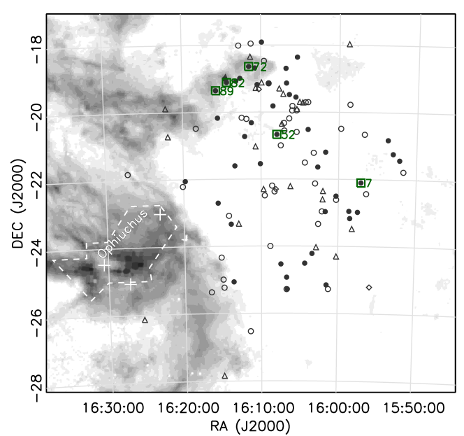
Figure 1: Distribution of our Upper Sco sources. We group full/evolved/transitional into protoplanetary disks (PDs: circles, filled for accreting CTTSs and open for WTTSs), debris/evolved transitional into debris disks (DBs: triangles), and separate sources with no disks (NDs: diamonds), see Sect. 4.1 and 4.2 for details. Green boxes mark sources with HVC emission in the [O I] $\lambda$6300 line (Sect. 5). Sources are overplotted on the cumulative dust extinction map out to 300 pc produced by Green et al. (2019). The white dashed polygon indicates the boundary between Ophiuchus and Upper Sco from Esplin et al. (2018). According to this boundary, three sources (white plus symbols) could be members of Ophiuchus, hence are not considered in the analysis.

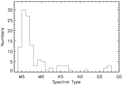
Figure 2: Distribution of spectral types for our Upper Sco sample.

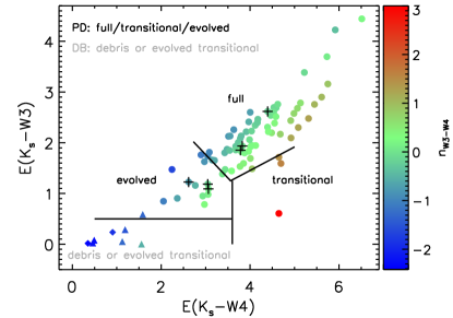
Figure 3: Extinction-corrected $K_{\rm s}$-W3 and $K_{\rm s}$-W4 color excesses for Upper Sco sources with photometric uncertainty $\leq$0.2 mag in $K_{\rm s}$, W3, and W4 bands. Symbols are color-coded by their $n_{\rm W3-W4}$ spectral index. Filled/empty symbols are for H$\alpha$ accreting/non-accreting stars (see Sect. 4.2). The black solid lines show the disk classification boundaries adopted in Luhman (2022). The plus symbols mark the 6 sources classified in this work, other symbols as in Figure 1.

2 Sample and Data Reduction

2.1 Sample

Although this study is directed toward Upper Sco sources with disks, at an age of 5-10 My the majority of young stars in this region have already lost their disks. Indeed, Luhman (2022) finds that only approximately 20% of the Upper Sco population still retain protoplanetary disks.

We start from a sample of 118 Upper Sco candidates that have Keck/HIRES high-resolution spectra covering the [O I] $\lambda$6300 transition. Figure 1 shows their distribution over the sky. Based on the boundary between Ophiuchus and Upper Sco identified in Esplin et al. (2018), three sources are likely Ophiuchus rather than Upper Sco members (white crosses in Figure 1). Thus, we remove them from our sample, leaving 115 Upper Sco sources analyzed in this work (see Table 7).

Most of the observations were collected based on evidence of the sources having full or transitional disks following the spectral energy distribution (SED) convention as in Espaillat et al. (2014), with the aim to complement ongoing ALMA observations of the disks. Of the 115 sources, 95 had been identified as disk candidates by Carpenter et al. (2006) based on Spitzer, or Luhman & Mamajek (2012) based on WISE excess emission, with 67 of them part of the ALMA disk survey by Barenfeld et al. (2016). Two of the objects (HD 143006 and AS 205A, IDs 11 and 72, respectively in Table 7) were already analyzed in Fang et al. (2018). Our sample also includes another 20 Upper Sco stars with Keck/HIRES spectra taken for other reasons (such as suspected binarity or interesting lightcurve morphology) that also have WISE photometry indicative of disks (see Sect. 4.1). Fourteen of them are not present in Luhman & Mamajek (2012) but collected in Luhman (2022).

Among our sample of 115 disk candidates, 104 have Gaia Early Data Release 3 (EDR3) parallactic distances from the geometric-distance table provided by Bailer-Jones et al. (2021). With these new distances, we noted that Source ID 19 has a much larger EDR3 distance than the mean distance of $\sim$142 pc to Upper Sco but also a large renormalized unit weight error (RUWE$=$14.338). This suggests that Source ID 19 is a multiple system or may otherwise be problematic in terms of the astrometric measurement. Thus, for ID 19, as well as the other 11 sources without Gaia parallaxes, we take the mean distance of 142 pc to Upper Sco estimated from the other members considered in this work.

2.2 Observations and data reduction

The spectral data for our sample are collected from the Keck/HIRES archive and cover observations carried out from 2006 to 2015. An observation log is provided in Table 2 of Appendix A. The table includes the dates of the observations, nominal spectral resolution, Program ID, and principle investigator. The nominal resolution for our sample is almost always 34,000 ($\Delta v\sim 8.8$ km/s). We estimate the spectral resolution near the [O I] $\lambda$6300 line by fitting 4 telluric lines around this transition toward 6 sources observed at high signal to noise (larger than 30). From the FWHM of the telluric lines we obtain a slightly better resolution of 7  km s^-1, which is used hereafter. This is essentially the same resolution achieved in our previous [O I] studies of young star-forming regions as measured in Pascucci et al. (2015).

We reduced the raw data using the Mauna Kea Echelle Extraction (MAKEE) pipeline written by Tom Barlow. MAKEE is designed to run non-interactively using a set of default parameters, and carry out bias-subtraction, flat-fielding, and spectral extraction, including sky subtraction, and wavelength calibration with ThAr calibration lamps. The wavelength calibration is performed in air by setting the keyword “novac” in the pipeline inputs. Heliocentric correction is also applied to the extracted spectra.

We corrected for the telluric contamination near the [O I] $\lambda$6300 line using the same method as in Fang et al. (2018). In short, we first remove any telluric absorption near the [O I] $\lambda$6300 line using O/B telluric standards; a detailed description of telluric removal can be found in the HIRES Data Reduction manual.

3 Stellar Parameters

3.1 Spectral classification and stellar properties

We classify the Keck spectra of each Upper Sco source using the grid of pre-main sequence spectral templates collected from the VLT/X-Shooter instrument (Manara et al., 2013, 2017a; Rugel et al., 2018). The spectral templates have been re-classified using the scheme for M types from Luhman (1999); Luhman et al. (2003); Luhman (2004, 2006), and for K and earlier types from Pecaut & Mamajek (2013), see a detailed description in Fang et al. (2021). We normalized the Keck spectra and the spectral templates in the same way, and find the template that best matches each Keck spectrum. We also derive the extinction toward each target using the best-fit template that reproduces the the Gaia photometry.

In our approach we fit 2 free parameters: the extinction in the $V$ band ($A_{V}$) and the absolute flux density at 7500 Å ($I_{\rm 7500}$). First, we redden the template with $A_{V}$ using the extinction law from Cardelli et al. (1989), adopting a total to selective extinction value typical for the interstellar medium ($R_{V}$=3.1). The reddened template is normalized to be one at 7500 Å and then multiplied by $I_{\rm 7500}$. Next, the “flux-calibrated” template is used to produce the synthetic Gaia photometry. The best-fit parameters are derived by minimizing the difference between the synthetic Gaia photometry and the observed Gaia photometry using the $\chi^{2}$ method. In this way, we can obtain both the extinction and continuum flux, estimated from the best-fit template, near the accretion-related lines and oxygen forbidden line, from which we can also estimate the line fluxes. A detailed description of the spectral classification and flux calibration is presented in Appendix B while a discussion of the flux calibration uncertainties is presented in Appendix C.

We obtain the effective temperature of each star from the spectral type to effective temperature relation in Fang et al. (2017). The stellar luminosity is estimated from $I_{\rm 7500}$ using the bolometric corrections from Herczeg & Hillenbrand (2014). We derive stellar masses from the luminosity and effective temperature using the non-magnetic pre-main sequence evolutionary tracks of Feiden (2016). A detailed description is presented in Appendix D. The resulting mass ($M_{\star}$), as well as the stellar spectral type, visual extinction ($A_{\rm V}$), luminosity ($L_{\star}$), and radius ($R_{\star}$) are listed in Table 7. Figure 2 shows the distributions of spectral types for our Upper Sco sample. The majority (69/115) of the sources are later than M3.

3.2 Stellar Radial velocity

We derive the stellar radial velocity (RV) by cross-correlating each spectrum with a stellar synthetic spectrum of the same effective temperature as our source. The model spectra are from Husser et al. (2013) for a solar abundance and surface gravity log $g$=4.0. We degrade the model spectrum to match the spectral resolution of HIRES, and rotationally broaden it to match the source photospheric features. We did the cross-correlation separately for each echelle order without strong emission lines and excluding the wavelength ranges with strong telluric absorption. The total number of available orders varies from source to source but it is at least 4 and up to 17. The resulting RVs for individual sources are listed in Table 7. The typical RV uncertainty is $\sim$1.4  km s^-1.

Since arc calibration frames for the absolute wavelength solution were taken only at the beginning of each night, systematic shifts of the wavelength solution of individual spectra are possible. In Fang et al. (2018), we assessed the shifts by cross-correlating the telluric lines with the model atmospheric transmission curve for the Keck Observatory, and found that the wavelength calibration tended to be drifted throughout the night by $\sim$0.5–2 km s^-1. In the same way, we estimate the shift for each observation and list the RV correction in Table 7. The RV of each source need to be corrected by adding the value in the “Correction” column to its RV. The shift only changes the heliocentric RV derived from the spectra, and does not affect the relative shift between the stellar photospheric absorption features and the [O I] $\lambda$6300 line.

4 Disk Types and Accretion

4.1 Disk classification

As mentioned in Sect. 2.1 our sample is drawn from disk candidates from Barenfeld et al. (2016) and our own SED classification. Because the majority (109 out of 115) of our Upper Sco sources have been recently assigned a disk classification by Luhman (2022) we use their classification for the 109 sources and follow his approach to classify the remaining 6 sources for a homogeneous re-classification. Luhman (2022) uses colors, particularly in the WISE bands, to distinguish 5 groups: Class III or diskless; debris/evolved transitional disks; evolved disks; transitional disks; and full disks. Figure 3 shows the boundaries of this classification in an extinction-corrected color excess plot where our sources are color-coded by their W3-W4 spectral index, calculated as $n=dlog(\lambda F_{\lambda})/dlog\lambda$. The used WISE photometry are collected from AllWISE Source Catalog (Cutri et al., 2021).

To simplify the discussion and more readily compare our results with those in younger star-forming regions, we adopt only 3 categories in this work: No disk (ND), Debris Disk (DB), and Protoplanetary Disk (PD). These 3 categories correspond to the Class III, the debris/evolved transitional disks, and the evolved/transitional/full disks in Luhman (2022), respectively. For the remaining 6 sources (IDs 99, 102, 105, 107, 108, 112; the plus symbols in Figure 3) without classification in Luhman (2022), we adopt the same approach and find that all of them are PDs. Based on this classification, our sample includes 4 ND sources, 24 DBs, and 87 PDs. The spectral energy distributions (SEDs) of these sources are shown in Appendix E.

We also include in Figure 3 a color bar indicating the magnitude of the WISE W3-W4 spectral index, as we will compare this index with the kinematic properties of the [O I] $\lambda$6300 line (see Sect. 5.5). Note that although there is only one bona-fide transition disk in our sample, there is a clear gradient in the W3-W4 color as the $K_{s}-W4$ excess increases in full and evolved disks.

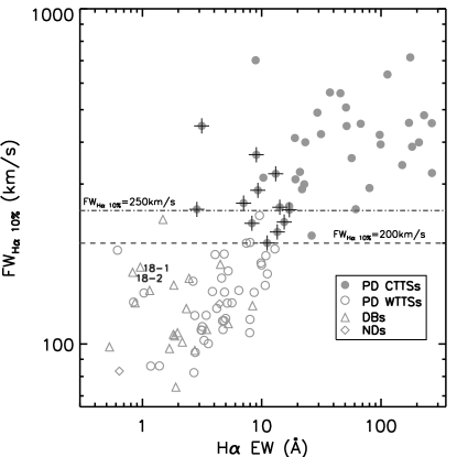
Figure 4: H$\alpha$ $FW_{\rm H\alpha 10\%}$ vs. $EW$ for our Upper Sco sample: filled circles for PDs classified as CTTSs; open circles for PDs classified as WTTSs; open triangles for the DBs; and open diamonds for NDs. The black pluses mark the 12 additional sources which were classified as WTTSs based on their H$\alpha$ $EW$, but re-classified as CTTSs based on their $FW_{\rm H\alpha 10\%}$.

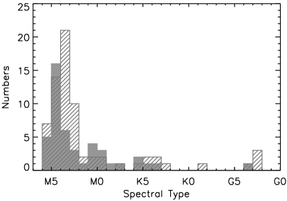
Figure 5: Distributions of spectral types for the CTTSs (grey color filled histograms) and WTTSs (grey line-filled histograms).

4.2 CTTS/WTTS classification

To identify which sources are truly accreting, we use two quantities: the H$\alpha$ equivalent width ($EW$) and the full width of the H$\alpha$ line at 10% of the peak intensity ($FW_{\rm H\alpha,10\%}$), which are commonly employed as accretion indicators (Barrado y Navascués & Martín, 2003; Jayawardhana et al., 2003; White & Basri, 2003; Natta et al., 2004; Fang et al., 2009, 2013). First, we classify young stars into accreting or non-accreting using the spectral type dependent H$\alpha$ $EW$ criteria described in Fang et al. (2009). Next, we check their $FW_{\rm H\alpha,10\%}$ and assign accreting (CTTS) status to those sources using the criteria defined in Appendix F, even if their H$\alpha$ $EW$ is below the accreting thresholds. This way sources with low H$\alpha$ $EW$s but broad profiles typical to accreting stars (12 in our sample) are properly classified as CTTS. The resulting classification is summarized in Table 7.

In Figure 4, we show the H$\alpha$ $FW_{\rm H\alpha,10\%}$ vs. $EW$ for our sample and mark the CTTSs we have identified. Source 18 is a known eclipsing binary (see USco 48 in David et al. 2019b for details) and its disk is classified as a DB. Its HIRES spectrum shows two well-separated H$\alpha$ emission lines whose $EWs$ and $FW_{\rm H\alpha,10\%}$ are consistent with WTTSs (see 18-1 and 18-2 in Figure 4).

Our study covers 32 sources with X-Shooter spectra whose accretion status has been recently determined by Manara et al. (2020). Taking advantage of the broad spectral coverage of X-Shooter, Manara et al. (2020) estimate the accretion luminosity by simultaneously fitting the stellar photosphere and Balmer continuum emission and classify a source as CTTS if its accretion luminosity is above the typical chromospheric value corresponding to its spectral type (see also Manara et al. 2017a). Among the 32 sources in common, 26 have our same classification and are not discussed further while 6, mostly low accretors, have a different classification. Recently, Thanathibodee et al. (2022) proposed a new scheme to classify low accretors using the He I $\lambda$10830 line profile. According to this scheme, IDs 1, 20, 41, and 58 would be classified as in Manara et al. (2020) while IDs 81 and 91 would follow our classification, see a detail discussion in Appendix G.

Given that there is no clear preference between the two classifications among the 6 sources discussed above and that only 43% (50/115) of the Upper Sco sample have He I $\lambda$10830 data, we will adopt here the CTTS/WTTS classification based only on the H$\alpha$ line from the HIRES data. Based on this classification, our Upper Sco sample comprises 45 CTTSs (45 PDs) and 70 WTTSs (42 PDs, 24 DBs, and 4 NDs). Figure 5 shows the distributions of spectral types for the CTTSs and WTTSs. The K-S test returns a high probability that these spectral types are drawn from the same parent population (p=0.2). As noted above, low accretors and/or accretors with significant accretion variability might have HIRES H${\alpha}$ profiles similar to those of DBs, where H${\alpha}$ originates from chromospheric emission, and thus might be classified as WTTSs here. For those WTTSs, a PD classification and an [O I] $\lambda$6300 detection most mean that they are accreting at low levels.

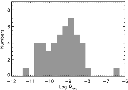
Figure 6: Distribution of Upper Sco CTTSs accretion rates.

4.3 Mass accretion rates

We estimate the accretion luminosity using four permitted emission lines covered by the HIRES spectra, two Balmer lines (H$\beta$, and H$\alpha$) and two He I lines (5876 and 6678Å), as their luminosities are known to be tightly correlated with the accretion luminosity (e.g., Herczeg & Hillenbrand 2008; Fang et al. 2009; Rigliaco et al. 2012; Alcalá et al. 2014, 2017). Line luminosities are derived from the measured equivalent widths of individual lines times the adjacent continuum flux, the latter is obtained from the template that best matches the Keck spectra and GAIA photometry of each target (see Sect. 3.1). We then convert line luminosities to accretion luminosities via the empirical relations in Fang et al. (2018). For two objects in common with Fang et al. (2018) (HD 143006 and AS 205A, IDs 11 and 72, respectively in Table 7) we collect mean accretion luminosities directly from that work. For an additional two sources accretion luminosities are only from the H$\alpha$ line. For the remaining 41 CTTSs in Upper Sco: 31 have mean accretion luminosities from the four permitted lines mentioned above; 8 from the H$\alpha$, H$\beta$, and He I$\lambda$5876 lines; and 2 only from the H$\alpha$ and H$\beta$ lines.

Finally, accretion luminosities are converted into mass accretion rates using the following relation (Gullbring et al., 1998):

$$\dot{M}_{\rm acc}=\frac{L_{{\rm acc}}R_{\star}}{{\rm G}M_{\star}(1-\frac{R_{\star}}{R_{\rm in}})},$$ (1)

where $R_{\rm in}$ denotes the truncation radius of the disk, which is taken to be 5 $R_{\star}$ (Gullbring et al., 1998), G is the gravitational constant, $M_{\star}$ is the stellar mass, and $R_{\star}$ is the stellar radius. The resulting mass accretion rates are also listed in Table 7 and their distribution is illustrated in Figure 6. The $Log~{}\dot{M}_{acc}$ in $M$_⊙ yr^-1 range from $-$11.3 to $-$6.6 and the medians for the Upper Sco sample is $-$9.3.

Table 3: [O I] $\lambda$6300 samples compared in this work. The SpTy range for the Warm sample is G0-M3 while for the Cool sample it is M3-M5.2.

Population	Age	Sample	$\Delta v$	Ref.	Median $L_{\rm acc}$	Median $\dot{M}_{\rm acc}$
	[Myr]		[km/s]		[L⊙]	[M⊙/yr]
SFB	1-3	Warm	6.6	1, 2, 3	0.04	3.6$\times$10-9
Cha+Lupus	1-3	Warm	16–40	4	0.02	2.3$\times$10-9
		Cool	16–40	4	0.0014	3.9$\times$10-10
NGC 2264	3-5	Warm	11.3	5	0.05	1.0$\times$10-8
Upper Sco	5-10	Warm	7	6	0.01	1.1$\times$10-9
		Cool	7	6	0.0009	2.3$\times$10-10

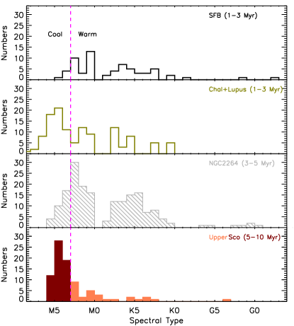
Figure 7: Distribution of spectral types for the SFB (black open histogram), Cha+Lupus (olive open histogram), NGC 2264 (gray line-filled histogram), and Upper Sco sample including only PDs.).

5 Mass Outflow Diagnosed via the [O I] $\lambda$6300 line

In the following subsections, we focus on the analysis of the [O I] $\lambda$6300  lines, their detection rates, line profiles, and relations between the [O I] $\lambda$6300 luminosity and stellar/disk properties. We focus on trends with spectral type and age, and throughout the analysis we compare our Upper Sco population with several other regions of recent star formation.

Specifically, the comparison samples are: the $\sim 1-3$ Myr old population of selected sources from Taurus, Lupus, $\rho$ Oph, and Corona Australis observed at high resolution ($R\sim 48,000$: Simon et al. 2016; Fang et al. 2018; Banzatti et al. 2019， hereafter SFB); the similarly young population of all disks in Chamaeleon I/II and Lupus observed at a much lower resolution with X-Shooter ($R\sim 7,400-18,200$: Nisini et al. 2018, hereafter Cha+Lupus); and the slightly older and further away ($\sim 3-5$ Myr, $d=760$ pc) population of NGC 2264 observed at intermediate resolution ($R\sim 26,500$: McGinnis et al. 2018). Figure 7 shows the distributions of the spectral type of these surveys that can be used for comparison with Upper Sco. As clearly shown in Figure 7, the $1-3$ Myr-old SFB and the $3-5$ Myr-old NGC 2264 populations have few sources later than M3. Thus, we split the Upper Sco sample into two subgroups: the ones later than M3 will be grouped into the Cool star sample while earlier spectral types (G0-M3) will constitute the Warm sample. Cool stars range in stellar mass from $\sim 0.08-0.28$ $M_{\odot}$ while Warm stars from $\sim 0.28-1.79$ $M_{\odot}$. Comparisons of the wind properties between the Upper Sco samples, the $1-3$ Myr-old SFB and the $3-5$ Myr-old NGC 2264 populations will be restricted to the G0-M3 spectral type range (Warm sample). A summary of these surveys used for the comparisons is provided in Table 3. The same table also gives the coverage in spectral type that can be used for comparison with Upper Sco.

We have verified that, within this restricted spectral type range (warm sample), the K-S test gives a high probability ($0.2-0.5$) that the stars in Upper Sco, SFB, and NGC 2264 are drawn from the same parent population. The Cha+Lupus survey covers a significant number of late-type stars and, as Upper Sco, two samples of Cool and Warm stars can be used for the comparison. The last two columns of Table 3 provide the median accretion luminosity and median mass accretion rate from each sample calculated in this work.

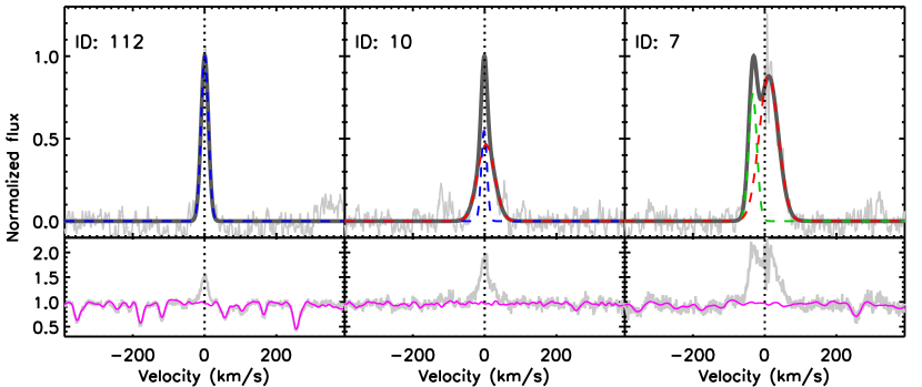
Figure 8: Examples of corrected [O I] $\lambda$6300 profiles as well their fits (top panels) and their uncorrected [O I] $\lambda$6300 profiles (bottom panels) with their photospheric corrections (shown in magenta), for three Upper Sco sources: SC (ID 109), NC+BC (ID 10, blue dashed line for NC and red dashed line for BC), and SCJ (ID 7, which shows both one SC and one HVC). SC dominates the Upper Sco sample (36/45) while there are only 7 BC+NC and just 2 SCJ, see Table 7. The gray solid line is the sum of the individual components. Line profile fits for all sources are shown in Fig. 24.

5.1 Line profiles and decomposition

We subtract photospheric features following the procedure outlined in Hartigan et al. (1989): a photospheric standard with spectral type similar to the target is rotationally broadened, veiled (parameter $r_{\lambda}$), and shifted in velocity to best match the photospheric lines of the target star. Veiling is used to mimic the filling effect in photospheric lines from the excess emission produced by the accretion shocks, and it is defined as the ratio of the excess continuum emission ($F_{\rm excess}$) to the photospheric flux ($F_{\rm phot}$): $r_{\lambda}=F_{\rm excess}/F_{\rm phot}$. The best-fit photospheric spectrum is achieved by minimizing the $\chi^{2}$, defined as $\chi^{2}=\sum(F_{\rm target}-F_{\rm Standard})^{2}$. Corrected line profiles are obtained by subtracting the best-fit photospheric spectra from the target spectra. Examples of corrected line profiles for three sources are shown in Figure 8 while all other line profiles are available in Figure 24 of Appendix E.

Following the same procedure used in our series of previous papers (Rigliaco et al., 2013; Simon et al., 2016; Fang et al., 2018; Banzatti et al., 2019), we decompose the [O I] $\lambda$6300 corrected line profiles into Gaussian components. To find the minimum number of Gaussians that describe the observed profile we use an iterative approach based on the IDL procedure mpfitfun. The minimum number is achieved when the root mean square (rms) of the residual (Gaussians minus original spectrum) is within 2$\sigma$ of the rms of the original spectrum next to the [O I] $\lambda$6300 line.

Figure 8 shows examples of the best-fit Gaussian components for profiles of three sources in Upper Sco. The other sources are shown in Appendix E, Figure 24. The best fit parameters resulting from the decomposition of each individual components, which are the line luminosities, the velocity centroid ($v_{\rm c}$), the full width at half maximum (FWHM), and the equivalent width (EW), are listed in Table 4 . The majority of LVC in Upper Sco are fit by single Gaussian components, with only a few BC+NC. For this reason we adopt the terminology for the [O I] $\lambda$6300 components as in Banzatti et al. (2019), so that LVC are either SC or BC+NC, as further discussed in Sect. 5.4.

The overall uncertainty of [O I] $\lambda$6300 line fluxes is about 0.08 dex including a flux calibration uncertainty of 15% in our Keck spectra and a median uncertainty of 12% in the line integration. For the line centroids and FWHMs, their median uncertainties of individual measurements are 1.3 and 1.5  km s^-1, respectively. The dominant uncertainty sources are the noise in the spectra of the Upper Sco sources and contamination from the residual of telluric [O I] $\lambda$6300 line, and the contribution in the uncertainty from the photospheric templates is negligible since these templates are always high quality and reproduce the photospheric features of the spectra of the Upper Sco sources very well (see Figs. 8 and 24.).

5.2 Detection rates

All of our 45 [O I] $\lambda$6300  detections in Upper Sco are from PD sources with a detection rate of 52% (45/87) among the PD; no emission is seen toward DB or ND sources. The majority of the detections (32/45, $\sim$71%) are from CTTSs but a considerable fraction (13/45, $\sim$29%) are associated with stars that appear not to be accreting based on their H$\alpha$ profiles, hence are classified as WTTSs in this work (see Appendix H). As we discuss in Sect. 5.4.2 the distribution of LVC centroids and FWHMs for CTTS and nominal WTTS with [O I] $\lambda$6300  is indistinguishable suggesting that the WTTS with [O I] detections are likely accreting CTTS but at levels below what can be discerned using H$\alpha$, see also Sect. 4.2.

Table 5 compares [O I] $\lambda$6300 detection statistics among CTTS and WTTS in Upper Sco with the younger regions in this comparative study, broken out by spectral type range, i.e. warm or cool samples and whether detections are in CTTS or sources classified as WTTS depending on H$\alpha$ properties. In order to compare [O I] $\lambda$6300 detection rates among the different regions, we use the Fisher exact test on a $2\times 2$ contingency table and test the null hypothesis that the number of [O I] $\lambda$6300 detections/non-detections in two populations is equally likely. The test returns the probability (p-value) of obtaining by chance a contingency table at least as extreme as the one that was actually observed. If the p-value is below 5% we conclude that the observed imbalance is statistically significant. The two contrasted populations are spectral ranges and evolutionary state and results are summarized in Table 6.

We start by exploring any spectral type (stellar mass) dependence. Here, the columns of the $2\times 2$ contingency table are the Warm and Cool samples, hence this test can be carried out only for Cha+Lupus and Upper Sco. For the 1-3 Myr-old Cha+Lupus sample (Nisini et al., 2018) the [O I] detection rates among CTTS are statistically indistinguishable: $\sim 75$% (50/67) for the Warm and $\sim 85$% (29/34) for the Cool CTTSs, Fisher p-value of 31%. The same is true for the 5-10 Myr-old Upper Sco region. Among the Warm sample [O I] detection rates are 50% (14/28) for CTTS and 64% (18/28) for CTTS+WTTS while among the Cool samples rates are 31% (18/59) and 46% (27/59), respectively. The Fisher p-values are 10% and 12% when considering CTTS or the combined CTTS+WTTS. Therefore, we conclude that the [O I] $\lambda$6300 line has a similar detection rate toward Warm (G0$-$M3) and Cool (M3$-$M5.2) stars.

Table 5: Summary of CTTS and WTTS in different samples with [O I] $\lambda$6300 detections.

Population	Sample	Total	CTTS		WTTS		CTTS+WTTS
				w[O I]		w[O I]	w[O I]
SFB	Warm	60	54	52	6	3	55
Cha+Lupus	Warm	67	62	50	5	0	50
	Cool	34	34	29	0	0	29
NGC 2264	Warm	165	165	104	0	0	104
Upper Sco	Warm	28	18	14	10	4	18
	Cool	59	27	18	32	9	27

Table 6: Results of the Fisher exact test. For each $2\times 2$ contingency table we report the percentage probability that the number of [O I] $\lambda$6300 detections/non-detections in two samples is equally likely.

Pop 1	Pop 2	CTTS	CTTS+WTTS
Warm Samples
Upper Sco	SFB	0.04	0.4
Upper Sco	Cha+Lupus	3	33
Upper Sco	NGC 2264	21	100
Cool Samples
Upper Sco	Cha+Lupus	3$\times 10^{-5}$	0.02
Cool vs. Warm Samples
Cha+Lupus		31	31
Upper Sco		10	12

In relation to evolutionary trends, we note that Table 5 indicates a decreasing [O I] detection rate with increasing age and decreasing accretion luminosity. To test if this trend is statistically significant, we construct $2\times 2$ contingency tables where one of the columns reports the number of Upper Sco [O I] $\lambda$6300 detections/non-detections while the other column gives the values for a younger region. Restricting ourselves to the Warm CTTS samples, we find that the imbalance between the Upper Sco [O I] detection rate (50%) and that of the 1-3 Myr-old SFB (87%) and Cha+Lupus (75%) regions is statistically significant, p-values of 0.04% and 3%. When including WTTS (CTTS+WTTS column), p-values increase to 0.43% and 33%, i.e. only the difference between SFB and Upper Sco remains statistically significant. However, among the Cool samples the [O I] detection rates for Upper Sco are statistically lower than those for Cha+Lupus for CTTS alone as well as CTTS+WTTS, p-values of $3\times 10^{-5}$ and 0.02%, respectively. The Fisher exact test reports high p-values of 21% and 100% when comparing the [O I] detection rates in the Warm samples of Upper Sco and NGC 2264. It is possible that the [O I] detection rate does not decrease from 3-5 Myr, the age of NGC 2264, to 5-10 Myr or, as pointed out in McGinnis et al. (2018), the lower rate in NGC 2264 is caused by the cluster larger distance in combination with strong nebular emission. In conclusion, we find strong evidence that [O I] $\lambda$6300 detection rate decreases going from 1-3 Myr-old regions to the 5-10 Myr-old sources in Upper Sco. Along with the [O I] detection rate the accretion luminosity decreases too and the K-S test returns a low probability (0.4%) for the Warm Upper Sco sample to be drawn from the same $L_{acc}$ population as the younger SFB and Cha+Lupus sources. The relation between the [O I] $\lambda$6300 and accretion will be further explored in the next subsection.

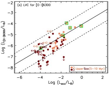
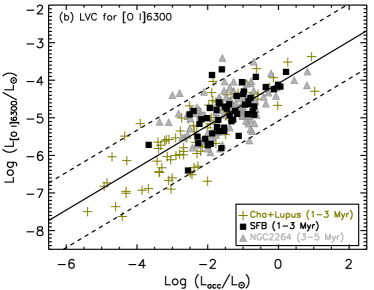
Figure 9: (a): LVC [O I] $\lambda$6300 luminosities vs accretion luminosities for the Upper Sco sample: filled(open) circles for CTTS(WTTS), orange(maroon) for Warm(Cool) sources. Green squares mark sources with HVCs in their [O I] $\lambda$6300 profiles. (b): LVC [O I] $\lambda$6300 luminosities vs accretion luminosities for other samples discussed in this work: black filled squares for the 1-3 Myr SFB, gray filled triangles for the 3-5 Myr NGC 2264, and olive pluses for the 1-3 Myr Cha+Lupus population. In each panel, the solid line is the best linear fit to all LVC detections for all the sample shown in both the panels. The dashed lines mark a $\pm$1 dex difference from the solid line.

5.3 Relation between the [O I] luminosity and accretion luminosity

Studies of young $\sim 1-3$ Myr old stars have shown that there exists a decent correlation between the accretion luminosity and the total [O I] $\lambda$6300  line luminosity, as well its individual HVC and LVC components (Rigliaco et al., 2013; Natta et al., 2014; Nisini et al., 2018; Fang et al., 2018). Our older Upper Sco [O I] $\lambda$6300 sample is dominated by LVC, hence we test whether a correlation between the [O I] $\lambda$6300 LVC luminosity and the accretion luminosity still persists at $\sim 5-10$ Myr.

Figure 9 (a) shows the [O I] $\lambda$6300 LVC luminosity vs accretion luminosity for our Upper Sco sample. Warm and Cool samples are identified by color and CTTS and WTTS by open and closed symbols. Upper limits for 13 CTTS without [O I] $\lambda$6300 and for 13 WTTS with [O I] $\lambda$6300 are also shown. In general the Upper Sco relation follows the same relation as the younger samples, which are shown in Figure 9 (b). The WTTS with [O I] $\lambda$6300 also follow the relation if the accretion upper limits are equated with a luminosity. An important question is whether these 13 nominal WTTS are misidentified by H$\alpha$ criteria and in fact are weakly accreting, as the CTTS/WTTs boundary is based on the width of this line, which can be ambiguous for diagnosing very low accretion rates (see Fig. 31). In contrast, in the Cha+Lupus sample accretion is measured via the Balmer jump rather than H$\alpha$ and thus includes sources with lower accretion luminosities than Upper Sco. In contrast, the CTTS without [O I] $\lambda$6300 lie somewhat below the LVC vs accretion luminosity relation and may indicate that accretion and [O I]are not uniquely coupled. Further discussion of the 13 PD WTTS with [O I] detection and the 13 CTTS with no [O I] detection is provided in Appendix H.

Figure 9 (b) summarizes results from the 1-3 Myr-old SFB, the similarly old Cha+Lupus, and the 3-5 Myr-old NGC 2264 populations. It is apparent that Upper Sco follows the same relation as the younger samples. The Pearson correlation coefficient is 0.78 for the [O I] $\lambda$6300 LVC luminosity vs accretion luminosity of the combined sample including only the CTTSs with [O I] $\lambda$6300 detection, with a low probability ($<10^{-16}$) that the two quantities are uncorrelated. We perform a two-variable linear regression including only the detections and obtain the following relation:

$$Log~{}L_{\rm OI63,LVC}=(0.56\pm 0.03)Log~{}L_{\rm acc}-(4.09\pm 0.06)$$ (2)

with a slope similar to those reported in the literature for younger samples, e.g., 0.52$\pm$0.07, 0.59$\pm$0.04, and 0.60$\pm$0.03 in Rigliaco et al. (2013), Nisini et al. (2018), and Fang et al. (2018), respectively.

5.4 Individual kinematic components

The identification of kinematic components within the LVC requires high spectral resolution ($R\geq 25,000$), hence the Cha+Lupus sample will not be included in the following comparison, however the 3-5 Myr-old NGC 2264 sample can be used. As we focus on [O I] $\lambda$6300 detections, we also include the nominal WTTS with [O I] $\lambda$6300 detections. In the discussion that follows we adopt the characterization of the LVC used by Banzatti et al. (2019), designating an LVC either as a BC+NC or SC. This necessitated re-assigning LVC from the literature previously designated as either BC or NC depending on their FWHM, into the single category SC (e.g., Simon et al., 2016; McGinnis et al., 2018).

5.4.1 HVC and LVC detection frequencies

High-velocity(HV) [O I] $\lambda$6300 emission at v$>30$ km/s is typically attributed to jets and low velocity (LVC) to slow disk winds (e.g., Hartigan et al. 1995; Lavalley-Fouquet et al. 2000; Bacciotti et al. 2000; Woitas et al. 2002; Simon et al. 2016; Fang et al. 2018; Banzatti et al. 2019). In our 45 [O I] $\lambda$6300 detections in Upper Sco we find only 5 sources with HVC, all of which also have LVC. Four of the HVC are among the highest accretion rate CTTS in the sample, as can be seen in Figure 9 green squares. Of the total 45 LVC profiles only 7 are BC+NC, 3 of which also have HVC, and the rest are fit with a single Gaussian, 2 of which also have HVC. Again following Banzatti et al. (2019), these are separately designated as SCJ or SC, with 2 of the former and 36 of the latter in Upper Sco. A comparison of profile types in the different regions is summarized in Table 7.

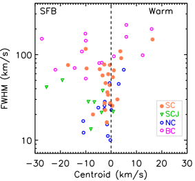
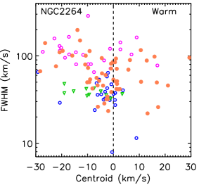
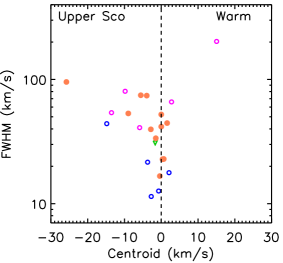
Figure 10: FWHM vs. centroids of various LVC components (SC, NC, BC, and SCJ) in the [O I] $\lambda$6300 line profiles for warm samples of three populations. In each panel, the orange filled circles are for the SC, blue open circles for the NC, magenta open circles for the BC, and the green upside down triangles for SCJ.

Table 7: Statistics on the line profiles including both the CTTS and WTTS

Population	SC	SCJ	BC+NC	HVC
Warm Samples (G0-M3)
SFB	44% (24/55)	16%  (9/55)	29% (16/55)	47% (26/55)
NGC 2264	52%(54/104)	21%(22/104)	22%(23/104)	31%(32/104)
Upper Sco	67%  (12/18)	6%  (1/18)	28%  (5/18)	22%  (4/18)
Cool Sample (M3-M5.2)
Upper Sco	89%(24/27)	4% (1/27)	7% (2/27)	4% (1/27)

The comparison in Table 7 shows that the frequency of HVCs decreases while that of SCs increases with age. We argue that this trend is actually due to the mass accretion rate which, overall, decreases with age (e.g., Table 3 and Hartmann et al., 2016). For example among the Warm sample, in Upper Sco (5-10 Myr-old) the median $\dot{M}_{acc}=1.1\times 10^{-9}~{}M_{\odot}~{}yr^{-1}$ while in SFB (1-3 Myr-old) and NGC 2264 (3-5 Myr-old) the medians are $\dot{M}_{acc}=3.6\times 10^{-9}~{}M_{\odot}~{}yr^{-1}$ and $\dot{M}_{acc}=1.0\times 10^{-8}~{}M_{\odot}~{}yr^{-1}$. In fact, within the three samples we also see that the median $L_{acc}$ for SC sources is always lower than that of BC+NC. For the Upper Sco Warm sample median $\dot{M}_{acc}$ are $3.5\times 10^{-9}$, $5.9\times 10^{-9}$, and $1.1\times 10^{-9}$ $M_{\odot}~{}yr^{-1}$ respectively for sources with HVC, BC+NC, and SC profiles. Thus, Upper Sco sources also follow the general trend in the [O I] $\lambda$6300 profile which simplifies and loses first the HVC and then the BC+NC as the mass accretion rate declines (e.g., Sect. 2.3 in Pascucci et al. 2022).

5.4.2 Distribution of LVC centroids and line widths

To further understand the evolution of the character of the LVC with age/accretion rate we show in Figure 10 the relation between the FWHM and centroid velocities of the BC, NC, SC, and SCJ for the warm samples in SFB, NGC 2264, and Upper Sco, where BC and NC are only from profiles with BC+NC. Because observations were carried out at slightly different spectral resolutions, we deconvolve all observed FWHMs for instrumental broadening taking a Gaussian FWHM appropriate for each sample (see Table 3). A summary of the corresponding median FWHMs and centroid velocities are listed in Table 8.

Several trends are apparent from Figure 10. In each region, the largest blueshifts are found among the components with the largest FWHM. These are predominantly the BC and SCJ components, but also some of the broader SC (which in previous works would also have been identified as BC). While the older Upper Sco follows the same trend, both the FWHM of the broadest lines and the $v_{\rm c}$ of the most blueshifted lines are less extreme. There are some redshifted components among the BC and broader SC, especially in NGC 2264, which are not well explained in a disk wind scenario, although they could arise from inclination effects (Simon et al., 2016). As seen in Table 8, for each population the median $v_{\rm c}$ of the SC is comparable to that of the corresponding NCs, i.e. less blue-shifted than BCs and SCJs.

Table 8: Median FWHMs ( km s^-1) and centroids ( km s^-1) of various LVC components

Population	SC	NC	BC	SCJ
Warm Samples (G0-M3)
SFB         $v_{\rm c}$	$-$1.3	$-$1.3	$-$7.4	$-$5.2
FWHM	55.9	24.0	98.7	28.2
NGC 2264 $v_{\rm c}$	$-$2.3	$-$2.4	$-$9.8	$-$9.8
FWHM	58.2	36.4	110.0	38.5
Upper Sco $v_{\rm c}$	$-$0.9	$-$2.7	$-$5.9	$-$1.7
FWHM	43.1	17.8	66.0	30.9
Cool Sample (M3-M5.2)
Upper Sco $v_{\rm c}$	$-$0.5	$\cdots$	$\cdots$	$\cdots$
FWHM	67.4	$\cdots$	$\cdots$	$\cdots$

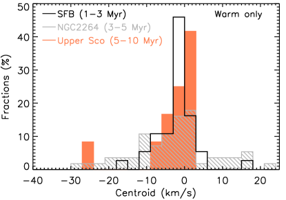
Figure 11: Distribution of centroids (Upper panel) and FWHMs corrected for instrumental broadening (Lower panel) for the [O I] $\lambda$6300 SCs around Warm (G0-M3) stars: orange color filled histogram for Upper Sco; black open histogram for the 1-3 Myr-old SFB; and gray line filled histogram for the 3-5 Myr-old NGC 2264 population. Centroids and FWHMs are statistically indistinguishable for the three samples, see text for details.

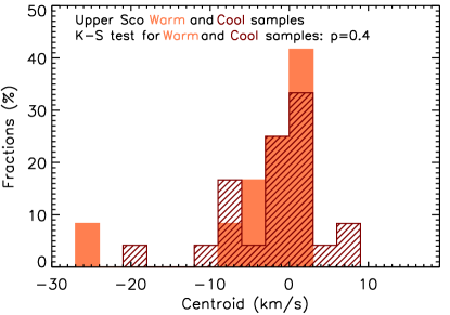
Figure 12: Distribution of centroids (Upper panel) and FWHMs corrected for instrumental broadening (Bottom panel) for the [O I] $\lambda$6300 SCs in Upper Sco (orange for the Warm and maroon line filled histogram for the Cool sample). Only FWHMs for the Warm and Cool samples are statistically different.

Since the majority of [O I] $\lambda$6300 in Upper Sco are SC profiles, especially among the Cool Sample, we confine the rest of the comparison to the SC parameters among the different populations. First we explore whether SC centroids ($\rm{v_{c}}$) and FWHMs change with spectral type and age. Figure 11 compares distributions of the $\rm{v_{c}}$ and FWHMs corrected for instrumental broadening for the Warm sources in the 1-3 Myr-old SFB, the 3-5 Myr-old NGC 2264, and our 5-10 Myr-old Upper Sco sample. As summarized in Table 8, the median $\rm{v_{c}}$ and FWHM for the three populations are: $-$1.3 km s^-1 and 55.9  km s^-1 for SFB, $-$2.3 km s^-1 and 58.2  km s^-1 for NGC 2264, and $-$0.9 km s^-1 and 43.1 km s^-1 for Upper Sco. Although the median values for Upper Sco are lower than in the younger regions, the K-S test returns high probabilities that the $\rm{v_{c}}$ and FWHMs are drawn from the same parent population (p$=0.27-0.97$ and 0.16$-$0.43, respectively).

Figure 12 focuses on comparing the Warm and Cool samples in Upper Sco, showing the distribution of SC $\rm{v_{c}}$ and FWHMs corrected for instrumental broadening, including both the CTTS and nominal WTTS with [O I] $\lambda$6300 detections. The median $\rm{v_{c}}$ and FWHM are $-$0.9  km s^-1 and 43.1  km s^-1 for the Warm sample while they are somewhat less blueshifted, $-$0.5  km s^-1 , and somewhat broader, 67.4  km s^-1 in the Cool sample. The K-S test returns a high probability that the SC centroids are drawn from the same parent population (p$=0.4$). In contrast, the K-S probability for their FWHMs is low (p$=0.047$) suggesting that Cool sources do have broader [O I] $\lambda$6300 lines than Warm ones.

These results suggest that the [O I] $\lambda$6300 in Upper Sco, which predominantly have a SC profile, is also tracing a slow disk wind as proposed for the young populations. We also note that, within each Upper Sco sample (Warm or Cool), CTTSs and WTTSs have indistinguishable distributions of centroids and FWHMs, suggesting that their [O I] $\lambda$6300 lines trace the same wind.

Next, we explore relations between the SC FWHM and disk inclination. Banzatti et al. (2019) reported a positive linear correlation between these two quantities for their mostly young sample of T Tauri stars with SpTy from M5 to G8. We repeat the test for all the sources with disk inclination in Upper Sco, SFB, and NCG 2264 (see Table 7) but correct their FWHMs for instrumental broadening given the different spectral resolutions of the surveys. For SFB, which is a subset of Banzatti et al. (2019), we find a Pearson’s correlation coefficient of 0.43 and a probability of 6%, slightly above the 5% cut that is typically adopted to indicate a correlation. The difference with the Banzatti et al. (2019) result can be attributed to the sample, here restricted to stars with SpTy no later than M3 and ages $\sim 1-3$ Myr. The Warm NGC 2264 sample does not show any hint for a positive correlation (even when we exclude the cluster of disks with inclinations of more than 80^∘, see Figure 13): the Pearson’s correlation coefficient and probability are $-$0.40 and 50% (0.26 and 16% when removing the disks with inclination larger than 90^∘). While the Warm Upper Sco sample is too small for such a test, the SC FWHM and disk inclination for the larger Upper Sco Cool sample are also not correlated (Pearson’s correlation coefficient and probability of 0.25 and 31%). We note however that Upper Sco disk inclinations have significant uncertainties, due to the relatively low sensitivity and resolution of the ALMA survey, while the NGC 2264 system inclinations were deduced from the star’s rotation properties. Interestingly, when combining all samples in Figure 13 and removing the suspicious clusters of disks at high inclinations ($>80^{\circ}$), the Pearson’s correlation coefficient and probability are 0.34 and 0.6%, hinting at a positive relation between the SC FWHM and disk inclination as reported in Banzatti et al. (2019).

When normalizing the FWHM by stellar mass, the relation between disk inclination and the SC FWHMs becomes more obvious (Figure 14). As for the young populations (Simon et al., 2016; Fang et al., 2018), the SC FWHM in Upper Sco increases with disk inclination, suggesting that Keplerian broadening contributes significantly to the line widths. Compared to Warm sources, Cool ones in Upper Sco tend to have larger normalized FWHMs, hinting at smaller emitting radii. Therefore, we estimate emitting radii and look for any difference with stellar mass. Following Fang et al. (2018), we calculate the emitting radius at the base of the wind ($r_{\rm base}$) from half of the deprojected [O I] $\lambda$6300 FWHM assuming Keplerian rotation. Figure 15 provides the distribution of $r_{\rm base}$ for these samples and highlights the smaller values for Cool stars: the median $r_{\rm base}$ for the Warm USco sample is 1.2 au while that for the Cool sample is 0.2 au. These radii are well within the so-called gravitational radius, the radius at which the sound speed equals the Keplerian orbital speed. Hence, these winds are not thermal/photoevaporative in origin (see also Simon et al. 2016).

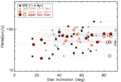
Figure 13: SC [O I] $\lambda$6300  FWHM vs. disk inclination for our Upper Sco sample (circles, orange for Warm and maroon for Cool sources, filled for CTTS and open for WTTS), the SFB 1-3 Myr sample (black filled squares), and the 3-5 Myr NGC 2264 population (gray filled triangles). FWHMs are corrected for instrumental broadening.

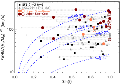
Figure 14: Same as Fig. 13 but that the FWHMs are corrected for instrumental broadening and normalized by stellar masses, and disk inclinations is shown in sin function. Blue dashed lines show Keplerian FWHM as a function of disk inclination at radii of 0.05, 0.2, 0.5, and 5 au.

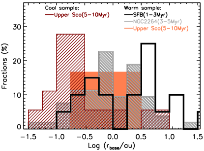
Figure 15: Distribution of emitting radii at the base of the wind for SFB (black open histogram), NGC 2264 (gray line-filled histogram), and Upper Sco (orange color/maroon line-filled histogram for Warm/Cool sources) disks with known inclinations, see Table 7. Cool sources have smaller emitting radii than Warm sources.

5.5 Relations with infrared spectral index

Previous work on $\sim 1-3$ Myr-old stars identified relations between the [O I] $\lambda$6300 EW/line luminosity as well as its FWHM and the infrared spectral index. In particular, Banzatti et al. (2019) showed that the SC [O I] $\lambda$6300 EW is anti-correlated with the $n_{13-31}$ index and Pascucci et al. (2020) reported a likely anti-correlation with the luminosity for a subset of the sample. Furthermore, Banzatti et al. (2019) found that the [O I] $\lambda$6300 FWHM is anti-correlated with $n_{13-31}$. These results have been interpreted as co-evolution of inner disks (larger $n_{13-31}$ indicate more depleted inner dust disks) and winds (lower [O I] $\lambda$6300 luminosities and smaller FWHM indicate less dense and further out winds). As 80% of the [O I] $\lambda$6300 detections in Upper Sco are SCs, we explore whether such relations persist at 5-10 Myr. However, as most Upper Sco sources lack low-resolution Spitzer spectra to compute the $n_{13-31}$ spectral index, we use instead the WISE W3 (12 µm) and W4 (22 µm) bands to generate an index as close as possible to the $n_{13-31}$.

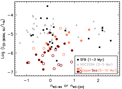
Figure 16: SC [O I] $\lambda$6300  luminosity vs. infrared spectral index for our Upper Sco sample (circles, orange for Warm and maroon for Cool sources, filled for CTTS and open for WTTS), the SFB 1-3 Myr sample (black filled squares), and the 3-5 Myr NGC 2264 population (gray filled triangles).The SC [O I] $\lambda$6300  luminosity is not correlated with these spectral indices.

Figure 16 shows the [O I] $\lambda$6300 line luminosity vs. $n_{\rm W3-W4}$ for our SC Upper Sco sample. As noted above, the Upper Sco sample is dominated by Cool stars and it is apparent from this figure that their [O I] $\lambda$6300 luminosity is lower than that of Warm stars and their disks cover a narrower $n_{\rm W3-W4}$ range. The Pearson’s r-test lends high probabilities that the two quantities are uncorrelated, 0.07 and 0.21 for the Warm and Cool samples, respectively.

In the same figure we also overplot the 1-3 Myr-old SFB (black squares) and the 3-5 Myr-old NGC 2264 (gray triangles) samples for which we have computed their spectral indices. Because of the large distance of NGC 2264 and possible contamination in the longest wavelength W4 band, we prefer the Spitzer 24 $\mu$m photometry (Sung et al., 2009) for this sample. The spatial resolution of Spitzer at 24 $\mu$m is two time higher than that of WISE/W4. Therefore for NCG 2264 we calculate the $n_{\rm W3-[24]}$ spectral index. The figure shows that the younger samples tend to have less dust-depleted disks and overall brighter [O I] $\lambda$6300 luminosities than the Upper Sco Warm sample. The Pearson’s r-test on the young samples also gives a high probability (0.12) that the two quantities are uncorrelated suggesting that a spectral index covering longer wavelengths, like $n_{13-31}$, can better link the depletion of inner disks with the [O I] $\lambda$6300 luminosity.

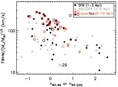
Figure 17: SC [O I] $\lambda$6300  FWHM vs. infrared spectral index. FWHMs are corrected for instrumental broadening and normalized by stellar masses. Symbols are the same as in Figure 16. The two quantities are anti-correlated.

Figure 17 shows the [O I] $\lambda$6300 FWHM normalized by stellar mass (see Sect. 3.1) vs. the $n_{\rm W3-W4}$ spectral index for our SC Upper Sco sample. The 1-3 Myr-old SFB and the 3-5 Myr-old NGC 2264 populations are also overplotted. Stellar masses for these samples are from the references in Table 3. Two trends are apparent: i) the Cool sample has larger FWHM normalized by stellar mass than the Warm sample and ii) the Cool and Warm samples follow the same anti-correlation between the logarithm of the FWHM normalized by stellar mass and spectral index reported for the younger samples. The Pearson’s correlation coefficients and probabilities for Upper Sco are -0.49 (0.11) and -0.48 (0.02) for the Warm and Cool samples, respectively. The insignificant correlation for the Warm sample is due to source ID 29. This source has a disk with a large cavity (radius$\sim$70 au) and a disk inclination close to face-on (6${}^{\circ}\pm 1.5^{\circ}$, Dong et al. 2017), and thus shows a narrow [O I] $\lambda$6300  profile. Excluding this source, the Pearson’s correlation coefficient and probability is $-$0.63 and 0.036 for the Warm Upper Sco sample. The same test on the younger samples combined lends a Pearson’s coefficient and probability of $-$0.50 and 3$\times 10^{-5}$. Hence, there is a statistically significant anti-correlation between the FWHM and the infrared spectral index.

6 [O I] results in broader context

6.1 The coevolution of accretion and disk winds

The past ten years have seen magnetized disk winds re-emerging as the prime driver of accretion, hence disk evolution, in what appears to be mostly low turbulence disks (e.g., Turner et al., 2014; Lesur et al., 2022; Pinte et al., 2022). In this paradigm, whenever MHD winds are present, stars accrete disk gas and the two phenomena, disk winds and accretion, are expected to coevolve. Upper Sco is a particularly interesting region to test this paradigm given its relatively old age and significant evolution of its disk population.

The analysis carried out in previous sections shows that the [O I] $\lambda$6300 line is a good MHD disk wind tracer in Upper Sco sources. First, the distribution of velocity centroids for the [O I] $\lambda$6300 SC profiles is asymmetric with a tail on the blueshifted side and a median of -0.9 km/s indicative of slow outflowing gas. Second, most SC FWHMs are broad enough (median of $\sim 43$ km/s) to be incompatible with a thermal wind (e.g., Simon et al. 2016 and Sect. 5.4.2). Furthermore, the distribution of SC velocity centroids and FWHMs from Upper Sco are indistinguishable from the full SC Warm sample, which covers an age range from $\sim 1-3$ Myr through to $\sim 5-10$ Myr.

As expected in the wind-driven accretion paradigm, we find that the well established correlation between the [O I] $\lambda$6300 luminosity and $L_{\rm acc}$ seen in younger regions is maintained by the older stars in Upper Sco, which have overall lower accretion rates. In the Warm Upper Sco sample the median $L_{\rm acc}$ is a factor of $\sim 3$ lower than Warm stars in SFB and Cha+Lupus (Sects. 5.2 and 5.3) and the Cool Upper Sco sample further extends this relation to the lowest $L_{\rm acc}$ (e.g., Figures 6 and 9). Thus, the connection between disk winds and accretion persists at $\sim 5-10$ Myr for stars that are still surrounded by accreting disks.

In addition to the [O I] $\lambda$6300 luminosity declining with $L_{\rm acc}$, the character of the [O I] $\lambda$6300 profiles evolves from a high frequency of HVC (jets) and LVC structure with both BC+NC at high $L_{\rm acc}$ to predominantly SC profiles, as seen here in Upper Sco and previously described in Pascucci et al. (2022). The transition of the LVC from BC+NC to SC is not yet understood and likely holds clues to the character of the disk wind as the accretion rate drops.

6.2 Wind mass loss versus mass accretion rates

Given that the [O I] $\lambda$6300 emission appears to trace a wind throughout disk evolution (e.g., Figure 11), here we use its properties to estimate wind mass loss rates from the modestly blueshifted SC components and explore whether there is any evidence of evolution in the wind mass loss vs. stellar accretion rate in these slow winds.

Following Fang et al. (2018) we assume that the [O I] $\lambda$6300 line is optically thin, traces gas at 5,000 K, and take an oxygen abundance of $3.2\times 10^{-4}$. With these assumptions the wind mass loss rate can be written as:

$$\dot{M}_{\rm loss}=2.4\times 10^{-4}\left(\frac{V_{\rm wind}}{10\,km/s}\right)\left(\frac{1\,au}{l_{\rm wind}}\right)\left(\frac{L_{6300}}{L_{\odot}}\right)\,M_{\odot}/yr$$ (3)

where $L_{6300}$ is the [O I] $\lambda$6300 luminosity while $V_{\rm wind}$ and $l_{\rm wind}$ are the wind velocity and height, respectively. As in Fang et al. (2018), the $V_{\rm wind}$ of each sub-sample is taken as the median value of the [O I] $\lambda$6300 centroids. In particular here we focus on the SCs and obtain $-$0.5 km s^-1 and $-$0.9 km s^-1 for the Upper Sco Warm and Cool samples, $-$1.5 km s^-1 for the Warm SFB sample, and $-$2.7 km s^-1 for the Warm NGC 2264 sample. The wind height is not constrained via high-resolution spectroscopy alone. Hence, as in Fang et al. (2018), we assume that it is a factor $f$ of the wind base ($r_{\rm base}$). This also means that the only sources for which we can estimate wind mass loss rates are those with a known disk inclination, i.e. those summarized in Table 7.

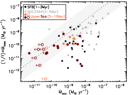
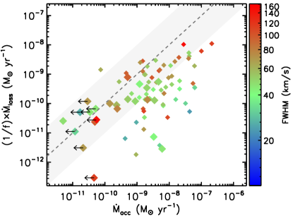
Figure 18: Top: $\dot{M}_{\rm loss}$ vs. $\dot{M}_{\rm acc}$ for the three populations. The symbols are same as in Figure 16. The dash line mark the y=x/10 relation, and the gray shaded region covers one order of mag difference on both sides around the y=x/10 relation. Bottom: Same as the top panel, but the symbols are coded with the [O I] $\lambda$6300 FWHMs.

Figure 18 shows the wind mass loss rate assuming $f=1$ as a function of the stellar mass accretion rate. For a wind vertical extent that is 10 (0.1) times $r_{\rm base}$, each point would shift down (up) by an order of magnitude. The dash line marks the one-to-one relation and the gray shaded region covers one order of magnitude difference on both sides. About 54% (43/84) of the sources fall within the gray shaded region where wind mass loss rates roughly match accretion rates. As reported in the Protostars and Planets VII chapter on disk winds, a similar ratio between ejection and accretion is found for the Class 0/I and II sources with spatially resolved outflows (Pascucci et al., 2022, for a recent review). We note that the older Upper Sco sources tend to have higher ratios between wind mass loss rates and accretion rates than younger samples. Among the Upper Sco sample, 79% (19/24) of the source fall within the gray shaded region in Figure 18, while among the younger sources there are only 51% of sources located within the shaded region and 47% of them have lower ratios (less than 0.01). We also note that the CTTS in Figure 18 with much lower $\dot{M}_{\rm loss}/\dot{M}_{acc}$ tend to have narrower SC profiles ($<40$ km/s), hence larger $r_{\rm base}$ and $l_{\rm wind}$ which lower $\dot{M}_{\rm loss}$ (Equation 3). This ratio could be higher if in these sources the bulk of the wind is molecular, hence any atomic tracer would only provide a lower limit to the mass loss rate (e.g., Pascucci et al., 2020). More work needs to be carried out to understand these high accreting stars with low $\dot{M}_{\rm loss}$ based on the [O I] $\lambda$6300 line.

6.3 [O I] $\lambda$6300 emitting radii and dust disk evolution

While covering a narrower $n_{\rm W3-W4}$ spectral index than Warm stars, Cool stars display the same anti-correlation between this index and the [O I] $\lambda$6300 FWHM corrected for stellar mass (Figure 17). In the context of the Warm sample, Furlan et al. (2009) find that $n_{\rm 13-31}\geq 1$ indicate disks with a large dust inner cavity, also called transition disks. Therefore, the anti-correlation has been interpreted as launching radii moving outward as the dust inner disk is depleted (Banzatti et al., 2019).

Although the Upper Sco sample includes only one bona-fide transition disk and that disk does not have an [O I] $\lambda$6300 detection, an increase in the W3-W4 spectral index still points to inner disk clearing (see Figure 3 and Sect. 4.1). Therefore, as in the younger samples, the Upper Sco data indicate that the [O I] $\lambda$6300 emitting radius, and possibly the wind launching radius, moves further out as the inner dust disk of both Warm and Cool stars is depleted.

7 Summary

We have analyzed high-resolution ($\Delta v\sim$ 7 km/s) optical spectra for a sample of 115 stars in the $\sim 5-10$ Myr-old Upper Sco association to search for potential signatures of disk winds via the [O I] $\lambda$6300 profiles. Of our sample, 87 are surrounded by a protoplanetary disk (here including full, evolved, and transition), 24 by a debris disk, and 4 have no disk. A total of 45 stars, all surrounded by a protoplanetry disk, are determined to be accreting (CTTS) based on H$\alpha$ profiles, with accretion rates ranging from $5\times 10^{-12}$ to $2.5\times 10^{-7}$ M_⊙/yr.

Our spectra cover a wide range of spectral types, from G0 to M5.2, with the majority later than M3. In order to facilitate comparison of [O I] $\lambda$6300 emission among stars of comparable mass in younger ($<5$ Myr-old) star-forming regions, we separate our sample into Warm (G0 to M3) and Cool (later than M3), corresponding to a boundary in stellar mass around 0.28 M_⊙. Two of the studies from younger regions which we use for comparison primarily consist of Warm stars at similar spectral resolution as our sample (NGC 2264 and a selection of stars from Taurus, Lupus, $\rho$ Oph and CrA). A third study includes both Warm and Cool stars but at lower spectral resolution (Cha + Lup). The Upper Sco dataset enables us to characterize [O I] $\lambda$6300 emission both as a function of age and as a function of stellar mass. Our main results can be summarized as follows:

1. The [O I] $\lambda$6300 line is detected in 45 out of 115 Upper Sco sources, all with protoplanetary disks. In general, The Upper Sco sample follows the same accretion luminosity$-$LVC [O I] $\lambda$6300 luminosity relation as the younger samples。 The decline of accretion luminosity with age is indicated by the fact that the median accretion luminosity of the warm Upper Sco sample is a factor of $\sim 3$ lower than that of younger stars when matched to the same spectral type range. The link between accretion and [O I] $\lambda$6300 may not be uniquely coupled however, as there are some CTTS with no [O I] $\lambda$6300 and some WTTS with [O I] $\lambda$6300. The possibility that these outliers may be due to sensitivity limits is discussed in the text.

2. All 45 [O I] $\lambda$6300 detections in Upper Sco show low velocity emission (LVC) and only 5 also show high velocity emission (HVC) attributed to a jet. Most LVC profiles are well fit by a single Gaussian (SC) but 7 show a composite form with both broad (BC) and narrow (NC) components.

3. As in other regions, the HVC and BC+NC are associated with higher accretion luminosities and their fraction in Upper Sco is lower than in younger regions with higher accretion luminosities. In contrast [O I] $\lambda$6300  in Upper Sco has the highest proportion of SC profiles.

4. In Upper Sco both the Warm and Cool samples have a distribution of LVC SC centroid velocities consistent with those in younger regions and as such are attributed to slow disk winds. While these components in all regions have smaller blueshifts than the BC or SCJ components, and are more comparable to the NC, their centroid distributions have modest median blueshifts and are asymmetric with a clear tail on the negative side.

5. The Upper Sco distribution of FWHM for the LVC SC differs between the Warm and Cool samples, with the Cool sample showing a larger FWHM normalized by stellar mass than the Warm one. If the lines are rotationally broadened this implies closer emitting radii (and perhaps wind launching) in lower mass stars. This comparison cannot yet be made for younger sources as the only study including low mass stars has a resolution too low for profile decomposition.

6. The Upper Sco [O I] $\lambda$6300 profiles show an anti-correlation between LVC SC FWHM and the WISE W3-W4 spectral index, following a similar trend reported for the younger samples. The correlation is in the sense that [O I] $\lambda$6300  profiles become narrower as the infrared spectral index increases. This index indicates inner disk clearing, although the only bona fide transition disk in the Upper Sco sample does not have an [O I] $\lambda$6300  detection.

Our main findings expand upon the emerging view of disk winds and their role in disk evolution in several ways. First, they demonstrate that disk winds persist at $\sim 5-10$ Myr, as long as stars are still accreting disk material. Second, as stars age and their accretion luminosity declines so does their [O I] $\lambda$6300 luminosity, in the same proportion as seen for younger stars. The character of the LVC tracing a disk wind evolves with decreasing accretion luminosity, where simple SC profiles with low wind velocities $\sim 1-2$ km s^-1 become the dominant mode in older regions like Upper Sco. The winds indicated by the SC components show a large spread in the ratio of mass loss rate to mass accretion rate, in some cases with ratios near unity but others with ratios less than 0.1. It is possible that in sources with low ratios (large accretion rates) the wind is mostly molecular and the [O I] $\lambda$6300  provides only a lower limit to the mass loss rate. Finally, all accreting stars, down to the late M types, present disk winds but the lowest mass stars differ from their Warm counterparts in the radii where [O I] $\lambda$6300 emission arises, where larger FWHM suggest smaller wind launching radii radii in the lower mass stars.

Table 1: A List of the Sources in This Work, as well as Their Stellar and Disk Properties

ID	Name	Dis	SpT	Log$L_{\star}$	$A_{\rm V}$	$R_{\star}$	Mass	Disk	CTTS	Log $\dot{M}_{\rm acc}$	$RV_{\rm Helio}$	Correction	Log$L_{\rm NC}$	Log$L_{\rm BC}$	Log$L_{\rm HVC}$	[O I]	LVC	HVC
		(pc)		($L_{\odot}$)	(mag)	($R_{\odot}$)	($M_{\odot}$)	Type		($M$⊙ yr-1)	( km s-1)	( km s-1)	($L_{\odot}$)	($L_{\odot}$)	($L_{\odot}$)	Det	Comp.
1	2MASSJ15514032-2146103	139.7	M4.8	$-1.39$	0.2	0.74	0.11	PD	N	$<-10.77$	$-4.9$	$-0.6$	$\cdots$	$-6.50$	$\cdots$	Y	SC
2	2MASSJ15521088-2125372	154.2	M4.9	$-2.70$	0.0	0.17	0.09	PD	Y	$-11.30$	$-4.7$	$-1.9$	$\cdots$	$-5.88$	$\cdots$	Y	SC
3	2MASSJ15530132-2114135	141.8	M4.7	$-1.41$	0.2	0.71	0.12	PD	Y	$-10.31$	$-5.3$	$-1.2$	$\cdots$	$-6.47$	$\cdots$	Y	SC
4	2MASSJ15534211-2049282	134.8	M3.8	$-1.27$	0.4	0.75	0.19	PD	Y	$-9.94$	$-6.0$	$-1.8$	$-6.24$	$-5.30$	$\cdots$	Y	BC+NC
5	2MASSJ15554883-2512240	143.0	G3.0	$0.37$	0.7	1.55	1.35	ND	N	$\cdots$	$-0.9$	$0.1$	$\cdots$	$\cdots$	$\cdots$	N
6	2MASSJ15562477-2225552	141.1	M4.2	$-1.30$	0.4	0.77	0.16	PD	N	$<-10.67$	$-5.0$	$-1.2$	$-6.56$	$\cdots$	$\cdots$	Y	SC
7	2MASSJ15570641-2206060	143.9	M4.8	$-1.46$	0.3	0.68	0.11	PD	Y	$-10.56$	$-5.2$	$-1.2$	$\cdots$	$-6.25$	$-6.66$	Y	SCJ	Y
8	2MASSJ15572986-2258438	142.0	M4.7	$-1.42$	0.2	0.71	0.12	PD	Y	$-10.59$	$-0.6$	$-1.1$	$\cdots$	$\cdots$	$\cdots$	N
9	2MASSJ15581270-2328364	144.9	G2.0	$0.51$	0.9	1.73	1.44	DB	N	$\cdots$	$-3.7$	$-1.0$	$\cdots$	$\cdots$	$\cdots$	N
10	2MASSJ15582981-2310077	140.0	M4.8	$-1.39$	0.7	0.74	0.11	PD	Y	$-8.92$	$-4.5$	$-1.5$	$-6.78$	$-6.38$	$\cdots$	Y	BC+NC
11	2MASSJ15583692-2257153	166.5	G3.0	$0.50$	0.4	1.80	1.52	PD	Y	$-7.99$	$-0.2$	$-1.3$	$-5.01$	$-4.44$	$\cdots$	Y	BC+NC
12	2MASSJ15584772-1757595	137.7	K3.0	$0.11$	1.5	1.83	1.25	DB	N	$<-9.95$	$-6.3$	$-0.8$	$\cdots$	$\cdots$	$\cdots$	N
13	2MASSJ16001330-2418106	146.2	K9.9	$-0.56$	0.5	1.22	0.56	DB	N	$<-10.23$	$-4.3$	$-0.5$	$\cdots$	$\cdots$	$\cdots$	N
14	2MASSJ16001730-2236504	144.0	M3.7	$-0.95$	0.0	1.07	0.21	PD	N	$<-10.00$	$-5.1$	$-1.9$	$\cdots$	$\cdots$	$\cdots$	N
15	2MASSJ16001844-2230114	168.1	M5.2	$-1.00$	0.4	1.20	0.11	PD	Y	$-8.22$	$-2.6$	$-1.3$	$-5.86$	$\cdots$	$\cdots$	Y	SC
16	2MASSJ16014086-2258103	135.0	M4.0	$-1.12$	0.0	0.92	0.18	PD	Y	$-8.46$	$-5.2$	$-1.0$	$\cdots$	$-5.51$	$\cdots$	Y	SC
17	2MASSJ16014157-2111380	140.3	M5.0	$-1.65$	1.0	0.56	0.09	PD	Y	$-9.85$	$-7.3$	$-1.0$	$\cdots$	$-6.36$	$\cdots$	Y	SC
18	2MASSJ16020039-2221237	141.4	M2.0	$-0.45$	0.2	1.62	0.33	DB	N	$<-9.38$	$-6.7$	$-0.9$	$\cdots$	$\cdots$	$\cdots$	N
19	2MASSJ16020287-2236139	142.0	M0.7	$-1.61$	0.4	0.39	0.53	DB	N	$\cdots$	$4.6$	$-0.3$	$\cdots$	$\cdots$	$\cdots$	N
20	2MASSJ16020757-2257467	139.6	M2.5	$-0.86$	0.3	1.05	0.31	PD	N	$<-10.28$	$-4.5$	$-0.9$	$\cdots$	$-5.75$	$\cdots$	Y	SC
21	2MASSJ16024152-2138245	139.4	M4.9	$-1.55$	0.0	0.63	0.09	PD	Y	$-9.94$	$-6.8$	$-0.8$	$\cdots$	$\cdots$	$\cdots$	N
22	2MASSJ16025123-2401574	144.5	K5.0	$-0.34$	0.1	1.32	0.85	DB	N	$<-10.26$	$-5.0$	$-1.3$	$\cdots$	$\cdots$	$\cdots$	N
23	2MASSJ16030161-2207523	139.1	M5.1	$-1.69$	0.5	0.54	0.08	PD	N	$<-10.82$	$-4.9$	$-2.6$	$\cdots$	$\cdots$	$\cdots$	N
24	2MASSJ16031329-2112569	136.1	M4.9	$-1.45$	0.4	0.70	0.09	PD	N	$<-10.87$	$-5.5$	$-1.6$	$\cdots$	$\cdots$	$\cdots$	N
25	2MASSJ16032225-2413111	139.0	M3.9	$-1.01$	0.6	1.03	0.19	PD	Y	$-9.06$	$-5.7$	$-1.0$	$\cdots$	$-5.64$	$\cdots$	Y	SC
26	2MASSJ16035767-2031055	142.6	K5.1	$-0.20$	0.9	1.56	0.81	PD	Y	$-9.29$	$-5.9$	$-0.5$	$\cdots$	$-4.91$	$\cdots$	Y	SC
27	2MASSJ16035793-1942108	152.9	M2.7	$-0.94$	0.6	0.97	0.31	PD	N	$<-10.43$	$-1.9$	$29.5$	$\cdots$	$\cdots$	$\cdots$	N
28	2MASSJ16041740-1942287	152.8	M3.6	$-1.11$	0.4	0.89	0.22	PD	N	$<-10.46$	$-2.7$	$-0.9$	$\cdots$	$-6.13$	$\cdots$	Y	SC
29	2MASSJ16042165-2130284	144.6	K2.3	$-0.01$	1.4	1.49	1.25	PD	N	$<-10.34$	$-4.4$	$-0.9$	$-4.70$	$\cdots$	$\cdots$	Y	SC
30	2MASSJ16043916-1942459	149.6	M3.7	$-1.21$	0.2	0.80	0.20	DB	N	$<-11.13$	$-3.1$	$-0.4$	$\cdots$	$\cdots$	$\cdots$	N
31	2MASSJ16050231-1941554	152.6	M4.2	$-1.46$	0.6	0.64	0.15	DB	N	$<-11.50$	$-2.8$	$-1.6$	$\cdots$	$\cdots$	$\cdots$	N
32	2MASSJ16052459-1954419	151.2	M3.4	$-1.05$	0.3	0.93	0.24	DB	N	$<-10.74$	$-2.8$	$-0.5$	$\cdots$	$\cdots$	$\cdots$	N
33	2MASSJ16052556-2035397	143.5	M5.1	$-1.42$	0.4	0.74	0.10	PD	N	$<-10.63$	$-2.7$	$-0.7$	$\cdots$	$\cdots$	$\cdots$	N
34	2MASSJ16052661-1957050	142.0	M5.1	$-1.28$	0.0	0.87	0.09	PD	N	$<-10.32$	$-2.6$	$-1.1$	$\cdots$	$-6.82$	$\cdots$	Y	SC
35	2MASSJ16053215-1933159	151.3	M4.8	$-1.61$	0.4	0.57	0.10	PD	Y	$-9.38$	$-2.3$	$-1.7$	$\cdots$	$-6.51$	$\cdots$	Y	SC
36	2MASSJ16055863-1949029	151.1	M3.8	$-1.27$	0.1	0.76	0.19	PD	N	$<-10.66$	$-2.9$	$-0.8$	$\cdots$	$\cdots$	$\cdots$	N

References. — 1. Simon et al. (2016); 2. Fang et al. (2018); 3. Banzatti et al. (2019); 4. Nisini et al. (2018); 5. McGinnis et al. (2018); 6. this work

Note. — The NGC 2264 sample was selected to include only CTTS (McGinnis et al., 2018)

Note. — The only Cool sample that can be compared with Upper Sco is Cha+Lupus but the spectral resolution of this latter dataset is too low to distinguish different line profiles (see also Sect. 5.4), hence it is excluded here

Note. — The median values are calculated when there are more than three sources with such types, except for the SCJ (only 1 case) in Upper Sco.

Table 1: (continuued)

ID	Name	Dis	SpT	Log$L_{\star}$	$A_{\rm V}$	$R_{\star}$	Mass	Disk	CTTS	Log $\dot{M}_{\rm acc}$	$RV_{\rm Helio}$	Correction	Log$L_{\rm NC}$	Log$L_{\rm BC}$	Log$L_{\rm HVC}$	[O I]	LVC	HVC
		(pc)		($L_{\odot}$)	(mag)	($R_{\odot}$)	($M_{\odot}$)	Type		($M$⊙ yr-1)	( km s-1)	( km s-1)	($L_{\odot}$)	($L_{\odot}$)	($L_{\odot}$)	Det	Comp.
37	2MASSJ16060061-1957114	155.0	M4.2	$-1.16$	0.0	0.90	0.17	PD	N	$<-10.53$	$-3.4$	$-0.2$	$\cdots$	$\cdots$	$\cdots$	N
38	2MASSJ16061330-2212537	139.0	M3.6	$-0.72$	0.4	1.39	0.21	DB	N	$<-10.15$	$-4.9$	$-1.0$	$\cdots$	$\cdots$	$\cdots$	N
39	2MASSJ16062196-1928445	142.0	M0.9	$-0.45$	0.5	1.50	0.42	PD	Y	$-8.90$	$-2.8$	$-0.6$	$-5.47$	$-5.33$	$\cdots$	Y	BC+NC
40	2MASSJ16062277-2011243	152.1	M4.1	$-1.31$	0.3	0.75	0.17	PD	N	$<-10.93$	$-3.6$	$-1.0$	$\cdots$	$-6.65$	$\cdots$	Y	SC
41	2MASSJ16063539-2516510	137.4	M5.1	$-1.64$	0.0	0.58	0.08	PD	Y	$-10.70$	$-4.1$	$-1.5$	$\cdots$	$\cdots$	$\cdots$	N
42	2MASSJ16064102-2455489	151.8	M4.8	$-1.55$	1.0	0.62	0.09	PD	Y	$-9.64$	$-3.1$	$-0.9$	$\cdots$	$-6.08$	$\cdots$	Y	SC
43	2MASSJ16064115-2517044	150.8	M3.5	$-1.26$	0.5	0.74	0.22	PD	N	$<-11.06$	$-3.7$	$-0.5$	$\cdots$	$\cdots$	$\cdots$	N
44	2MASSJ16064385-1908056	145.3	K7.9	$-0.47$	0.5	1.24	0.69	PD	Y	$-9.95$	$-3.6$	$-2.1$	$\cdots$	$\cdots$	$\cdots$	N
45	2MASSJ16070014-2033092	138.3	M2.7	$-0.93$	0.6	0.99	0.31	PD	N	$<-11.21$	$-5.5$	$-1.5$	$-6.07$	$\cdots$	$\cdots$	Y	SC
46	2MASSJ16070211-2019387	145.6	M5.0	$-1.66$	0.5	0.55	0.09	PD	N	$<-10.86$	$-3.0$	$-0.3$	$\cdots$	$\cdots$	$\cdots$	N
47	2MASSJ16070873-1927341	147.7	M4.0	$-1.35$	0.5	0.71	0.17	DB	N	$<-11.05$	$-3.3$	$0.0$	$\cdots$	$\cdots$	$\cdots$	N
48	2MASSJ16071971-2020555	154.6	M3.8	$-1.16$	0.5	0.85	0.20	DB	N	$<-10.89$	$-2.4$	$-1.1$	$\cdots$	$\cdots$	$\cdots$	N
49	2MASSJ16072625-2432079	143.4	M3.9	$-0.93$	0.0	1.13	0.19	PD	Y	$-9.61$	$-2.7$	$-1.4$	$\cdots$	$-5.79$	$\cdots$	Y	SC
50	2MASSJ16072747-2059442	179.3	M4.9	$-0.89$	0.5	1.33	0.13	PD	N	$<-9.90$	$-5.6$	$-1.1$	$\cdots$	$\cdots$	$\cdots$	N
51	2MASSJ16073939-1917472	138.5	M2.7	$-0.82$	0.5	1.13	0.29	DB	N	$<-10.91$	$-4.8$	$-1.7$	$\cdots$	$\cdots$	$\cdots$	N
52	2MASSJ16075796-2040087	135.9	K4.0	$-0.96$	1.4	0.59	0.71	PD	Y	$-8.96$	$2.5$	$-1.9$	$\cdots$	$-3.97$	$-3.87$	Y	BC+NC	Y
53	2MASSJ16080555-2218070	143.5	M2.5	$-0.82$	0.4	1.10	0.31	ND	N	$<-10.16$	$-5.7$	$-0.8$	$\cdots$	$\cdots$	$\cdots$	N
54	2MASSJ16081566-2222199	138.6	M2.7	$-0.87$	0.3	1.06	0.30	PD	N	$<-10.52$	$-4.6$	$-2.2$	$\cdots$	$\cdots$	$\cdots$	N
55	2MASSJ16082751-1949047	142.0	M4.9	$-1.20$	0.6	0.93	0.11	PD	Y	$-9.76$	$-5.7$	$-1.0$	$\cdots$	$\cdots$	$\cdots$	N
56	2MASSJ16083455-2211559	137.9	M4.9	$-1.60$	0.4	0.59	0.09	PD	N	$<-11.21$	$-7.0$	$-0.8$	$\cdots$	$\cdots$	$\cdots$	N
57	2MASSJ16084894-2400045	143.5	M3.9	$-1.34$	0.1	0.71	0.18	PD	N	$<-11.11$	$-1.5$	$-1.1$	$\cdots$	$\cdots$	$\cdots$	N
58	2MASSJ16090002-1908368	135.7	M5.0	$-1.41$	0.2	0.74	0.10	PD	N	$<-10.40$	$-7.3$	$-1.4$	$\cdots$	$\cdots$	$\cdots$	N
59	2MASSJ16090075-1908526	136.9	M0.6	$-0.51$	0.9	1.36	0.46	PD	Y	$-8.92$	$-5.8$	$-0.9$	$\cdots$	$-5.04$	$\cdots$	Y	SC
60	2MASSJ16093558-1828232	157.4	M3.7	$-1.16$	1.0	0.85	0.21	PD	N	$<-10.27$	$-3.0$	$-1.0$	$\cdots$	$-6.14$	$\cdots$	Y	SC
61	2MASSJ16094098-2217594	144.8	K9.0	$-0.15$	0.5	1.86	0.56	DB	N	$<-9.77$	$-5.0$	$-0.8$	$\cdots$	$\cdots$	$\cdots$	N
62	2MASSJ16095361-1754474	157.1	M5.0	$-1.54$	0.4	0.63	0.10	PD	Y	$-10.26$	$-3.3$	$-1.0$	$\cdots$	$-6.86$	$\cdots$	Y	SC
63	2MASSJ16095441-1906551	137.6	M1.8	$-0.66$	0.9	1.26	0.35	DB	N	$<-10.25$	$-5.9$	$-1.0$	$\cdots$	$\cdots$	$\cdots$	N
64	2MASSJ16101473-1919095	137.9	M3.4	$-0.93$	0.6	1.06	0.24	ND	N	$<-11.26$	$-5.7$	$-0.7$	$\cdots$	$\cdots$	$\cdots$	N
65	2MASSJ16102819-1910444	150.4	M5.0	$-1.78$	0.2	0.48	0.08	PD	Y	$-10.80$	$-3.4$	$-0.8$	$\cdots$	$\cdots$	$\cdots$	N
66	2MASSJ16103956-1916524	155.0	M2.8	$-1.00$	0.6	0.92	0.30	DB	N	$<-10.35$	$-3.8$	$-2.3$	$\cdots$	$\cdots$	$\cdots$	N
67	2MASSJ16104202-2101319	140.1	K4.9	$-0.00$	1.3	1.93	0.79	DB	N	$<-9.54$	$-4.8$	$0.5$	$\cdots$	$\cdots$	$\cdots$	N
68	2MASSJ16104636-1840598	140.1	M4.9	$-1.52$	0.9	0.64	0.09	PD	Y	$-10.30$	$-5.6$	$-1.4$	$\cdots$	$\cdots$	$\cdots$	N
69	2MASSJ16111330-2019029	152.9	M4.3	$-0.98$	0.0	1.12	0.16	PD	Y	$-8.48$	$-2.4$	$-1.8$	$\cdots$	$-5.67$	$\cdots$	Y	SC
70	2MASSJ16111534-1757214	135.3	M1.2	$-0.55$	0.7	1.36	0.40	PD	N	$<-9.69$	$-5.7$	$-2.5$	$\cdots$	$-5.75$	$\cdots$	Y	SC
71	2MASSJ16112057-1820549	135.8	K4.8	$-0.09$	1.1	1.72	0.83	DB	N	$\cdots$	$-6.2$	$-1.1$	$\cdots$	$\cdots$	$\cdots$	N
72	2MASSJ16113134-1838259	131.7	K5.0	$0.89$	1.8	5.44	0.73	PD	Y	$-6.60$	$-5.3$	$-1.8$	$-4.62$	$-4.46$	$-4.09$	Y	BC+NC	Y
73	2MASSJ16115091-2012098	139.8	M3.8	$-1.15$	0.3	0.86	0.20	PD	N	$<-10.54$	$-6.8$	$NaN$	$\cdots$	$-5.83$	$\cdots$	Y	SC
74	2MASSJ16122737-2009596	142.2	M5.2	$-1.54$	1.0	0.65	0.08	PD	N	$<-10.74$	$-3.1$	$-1.4$	$\cdots$	$\cdots$	$\cdots$	N
75	2MASSJ16123916-1859284	134.7	M2.0	$-0.54$	0.9	1.47	0.33	PD	Y	$-8.69$	$-2.1$	$-2.7$	$\cdots$	$-5.49$	$\cdots$	Y	SC
76	2MASSJ16124893-1800525	152.0	M3.8	$-1.07$	0.2	0.95	0.20	PD	N	$<-10.82$	$-4.2$	$-3.4$	$\cdots$	$\cdots$	$\cdots$	N
77	2MASSJ16125533-2319456	152.5	G2.0	$0.78$	0.7	2.38	1.79	DB	N	$\cdots$	$-3.3$	$-0.4$	$\cdots$	$\cdots$	$\cdots$	N
78	2MASSJ16130996-1904269	135.1	M4.9	$-1.11$	1.2	1.04	0.12	PD	Y	$-8.93$	$-6.0$	$-0.4$	$\cdots$	$-5.55$	$\cdots$	Y	SC
79	2MASSJ16133650-2503473	142.0	M3.8	$-0.89$	1.3	1.17	0.20	PD	Y	$-8.33$	$-1.2$	$-0.6$	$\cdots$	$-5.27$	$\cdots$	Y	SC
80	2MASSJ16135434-2320342	142.0	M4.8	$-1.02$	0.0	1.13	0.13	PD	Y	$-8.20$	$-5.0$	$-3.2$	$\cdots$	$\cdots$	$\cdots$	N
81	2MASSJ16141107-2305362	142.0	K3.0	$0.50$	1.0	2.86	1.23	PD	N	$\cdots$	$-8.4$	$-1.2$	$\cdots$	$\cdots$	$\cdots$	N
82	2MASSJ16142029-1906481	138.8	K9.0	$-0.68$	2.2	1.02	0.67	PD	Y	$-9.04$	$-5.4$	$-1.2$	$-5.08$	$\cdots$	$-4.19$	Y	SCJ	Y
83	2MASSJ16142893-1857224	135.1	M3.2	$-0.73$	0.4	1.30	0.25	DB	N	$<-9.48$	$-4.6$	$-0.7$	$\cdots$	$\cdots$	$\cdots$	N
84	2MASSJ16143367-1900133	135.8	M3.3	$-0.45$	1.7	1.82	0.23	PD	Y	$-9.29$	$-7.0$	$-1.3$	$\cdots$	$-4.93$	$\cdots$	Y	SC
85	2MASSJ16145918-2750230	149.2	G8.0	$0.07$	0.7	1.33	1.24	DB	N	$\cdots$	$1.1$	$-0.6$	$\cdots$	$\cdots$	$\cdots$	N
86	2MASSJ16145928-2459308	157.7	M4.7	$-1.31$	0.2	0.80	0.12	PD	N	$<-10.78$	$-1.3$	$-2.3$	$\cdots$	$-6.62$	$\cdots$	Y	SC
87	2MASSJ16151239-2420091	145.2	M4.7	$-1.70$	0.8	0.51	0.10	PD	N	$<-11.23$	$-2.7$	$-1.4$	$\cdots$	$-6.47$	$\cdots$	Y	SC
88	2MASSJ16153456-2242421	136.9	M0.2	$-0.41$	0.3	1.49	0.48	PD	Y	$-8.68$	$-2.4$	$-0.8$	$\cdots$	$-5.14$	$\cdots$	Y	SC
89	2MASSJ16154416-1921171	125.9	K8.0	$-0.38$	2.0	1.38	0.66	PD	Y	$-8.23$	$-3.8$	$-4.0$	$-4.85$	$-4.57$	$-4.58$	Y	BC+NC	Y
90	2MASSJ16163345-2521505	158.4	M0.1	$-0.73$	1.2	1.02	0.56	PD	N	$<-10.91$	$0.0$	$-2.8$	$\cdots$	$\cdots$	$\cdots$	N
91	2MASSJ16181904-2028479	138.3	M5.0	$-1.47$	0.8	0.69	0.10	PD	N	$<-10.63$	$-5.2$	$-1.1$	$\cdots$	$\cdots$	$\cdots$	N
92	2MASSJ16215466-2043091	108.5	K7.0	$-0.35$	0.7	1.41	0.68	DB	N	$\cdots$	$-4.1$	$-2.0$	$\cdots$	$\cdots$	$\cdots$	N
93	2MASSJ16220961-1953005	133.3	M3.7	$-0.65$	0.8	1.53	0.20	DB	N	$<-10.12$	$-7.4$	$-0.7$	$\cdots$	$\cdots$	$\cdots$	N
94	2MASSJ16235385-2946401	134.6	G2.5	$0.66$	0.7	2.12	1.69	ND	N	$\cdots$	$0.5$	$-0.9$	$\cdots$	$\cdots$	$\cdots$	N
95	2MASSJ16270942-2148457	137.0	M4.9	$-1.70$	1.3	0.52	0.09	PD	N	$<-10.68$	$-5.4$	$-1.8$	$\cdots$	$\cdots$	$\cdots$	N
96	2MASSJ15564244-2039339	140.2	M3.4	$-1.05$	0.5	0.92	0.24	PD	N	$<-10.84$	$-4.9$	$-0.6$	$\cdots$	$\cdots$	$\cdots$	N
97	2MASSJ15583620-1946135	155.6	M3.9	$-1.16$	0.2	0.87	0.19	PD	N	$<-10.84$	$-2.3$	$-0.9$	$\cdots$	$\cdots$	$\cdots$	N
98	2MASSJ15594426-2029232	138.0	M4.2	$-1.18$	0.5	0.88	0.17	PD	N	$<-10.38$	$-6.3$	$-1.1$	$\cdots$	$\cdots$	$\cdots$	N
99	2MASSJ16011398-2516281	142.0	M4.1	$-1.13$	0.0	0.92	0.17	PD	N	$<-10.40$	$-1.8$	$-1.3$	$\cdots$	$\cdots$	$\cdots$	N
100	2MASSJ16012902-2509069	134.5	M4.2	$-1.21$	0.1	0.84	0.16	PD	Y	$-8.71$	$-5.1$	$-1.4$	$\cdots$	$-5.97$	$\cdots$	Y	SC
101	2MASSJ16023587-2320170	139.1	M3.7	$-1.07$	0.1	0.93	0.21	PD	N	$<-10.12$	$-5.6$	$-0.5$	$\cdots$	$\cdots$	$\cdots$	N
102	2MASSJ16041893-2430392	142.0	M2.7	$-0.52$	0.1	1.58	0.29	PD	Y	$-9.22$	$-4.9$	$-1.6$	$\cdots$	$-5.72$	$\cdots$	Y	SC
103	2MASSJ16052157-1821412	148.9	K3.8	$-0.04$	0.9	1.66	1.05	PD	Y	$-8.96$	$-3.5$	$-1.6$	$\cdots$	$-4.78$	$\cdots$	Y	SC
104	2MASSJ16064794-1841437	155.8	K9.0	$-0.17$	0.8	1.83	0.56	PD	Y	$-9.42$	$-2.1$	$-1.2$	$\cdots$	$\cdots$	$\cdots$	N
105	2MASSJ16093164-2229224	153.9	M2.5	$-0.48$	0.5	1.63	0.30	PD	N	$<-9.63$	$-2.7$	$-1.3$	$\cdots$	$\cdots$	$\cdots$	N
106	2MASSJ16100501-2132318	145.4	K9.0	$-0.42$	0.6	1.37	0.61	PD	Y	$-8.63$	$-4.3$	$-1.3$	$-5.45$	$\cdots$	$\cdots$	Y	SC
107	2MASSJ16112601-2631558	142.0	M2.6	$-0.72$	0.4	1.25	0.29	PD	N	$<-10.18$	$-4.1$	$-1.6$	$\cdots$	$\cdots$	$\cdots$	N
108	2MASSJ16120505-2043404	122.5	M1.5	$-0.57$	1.0	1.37	0.37	PD	Y	$-9.50$	$-5.6$	$-1.3$	$\cdots$	$\cdots$	$\cdots$	N
109	2MASSJ16120668-3010270	131.9	M0.0	$-0.59$	0.3	1.19	0.55	PD	Y	$-9.40$	$-1.3$	$-1.5$	$-5.35$	$\cdots$	$\cdots$	Y	SC
110	2MASSJ16132190-2136136	144.8	M3.3	$-0.87$	0.5	1.12	0.25	PD	Y	$-9.51$	$-3.4$	$-0.6$	$\cdots$	$\cdots$	$\cdots$	N
111	2MASSJ16145244-2513523	160.0	M3.5	$-1.09$	0.5	0.90	0.23	PD	N	$<-10.33$	$-2.6$	$-1.5$	$\cdots$	$\cdots$	$\cdots$	N
112	2MASSJ16153220-2010236	142.0	M2.4	$-0.57$	1.0	1.46	0.31	PD	Y	$-9.13$	$-6.7$	$-1.8$	$\cdots$	$\cdots$	$\cdots$	N
113	2MASSJ16194711-2203112	126.8	M4.2	$-1.30$	0.1	0.77	0.16	PD	Y	$-10.30$	$-3.3$	$-1.7$	$\cdots$	$\cdots$	$\cdots$	N
114	2MASSJ16200616-2212385	137.3	M3.6	$-1.22$	0.2	0.78	0.21	PD	N	$<-11.23$	$-2.2$	$-1.2$	$\cdots$	$\cdots$	$\cdots$	N
115	2MASSJ16252883-2607538	139.5	M3.1	$-0.87$	0.4	1.10	0.27	DB	N	$<-10.44$	$-3.1$	$-1.9$	$\cdots$	$\cdots$	$\cdots$	N

Table 2: Observation log summary

ID	Name	RA	DEC	Data-Obs	Nominal	Program	PI	S/N
		(J2000)	(J2000)		Resolution	ID
1	2MASSJ15514032-2146103	15 51 40.32	$-$21 46 10.3	2013-06-04	34000	C189Hr	Carpenter	9.1
2	2MASSJ15521088-2125372	15 52 10.88	$-$21 25 37.2	2015-06-02	34000	C247Hr	Carpenter	1.0
3	2MASSJ15530132-2114135	15 53 01.32	$-$21 14 13.5	2013-06-04	34000	C189Hr	Carpenter	6.8
4	2MASSJ15534211-2049282	15 53 42.11	$-$20 49 28.2	2006-08-12	45000	H212Hr	Shkolnik	3.2
5	2MASSJ15554883-2512240	15 55 48.83	$-$25 12 24.0	2015-06-01	34000	C247Hr	Carpenter	40.3
6	2MASSJ15562477-2225552	15 56 24.77	$-$22 25 55.2	2007-05-24	34000	C269Hr	Dahm	16.4
7	2MASSJ15570641-2206060	15 57 06.41	$-$22 06 06.0	2007-05-25	34000	C269Hr	Dahm	10.7
8	2MASSJ15572986-2258438	15 57 29.86	$-$22 58 43.8	2007-05-25	34000	C269Hr	Dahm	16.4
9	2MASSJ15581270-2328364	15 58 12.70	$-$23 28 36.4	2015-06-01	34000	C247Hr	Carpenter	38.4
10	2MASSJ15582981-2310077	15 58 29.81	$-$23 10 07.7	2007-05-24	34000	C269Hr	Dahm	14.8
11	2MASSJ15583692-2257153	15 58 36.92	$-$22 57 15.3	2008-05-23	48000	C199Hb	Herczeg	57.3
12	2MASSJ15584772-1757595	15 58 47.72	$-$17 57 59.5	2015-06-01	34000	C247Hr	Carpenter	38.1
13	2MASSJ16001330-2418106	16 00 13.30	$-$24 18 10.6	2015-06-02	34000	C247Hr	Carpenter	30.5
14	2MASSJ16001730-2236504	16 00 17.30	$-$22 36 50.4	2015-06-01	34000	C247Hr	Carpenter	20.0
15	2MASSJ16001844-2230114	16 00 18.44	$-$22 30 11.4	2015-06-01	34000	C247Hr	Carpenter	10.6
16	2MASSJ16014086-2258103	16 01 40.86	$-$22 58 10.3	2013-06-04	34000	C189Hr	Carpenter	12.4
17	2MASSJ16014157-2111380	16 01 41.57	$-$21 11 38.0	2013-06-04	34000	C189Hr	Carpenter	2.8
18	2MASSJ16020039-2221237	16 02 00.39	$-$22 21 23.7	2015-06-02	34000	C247Hr	Carpenter	13.8
19	2MASSJ16020287-2236139	16 02 02.87	$-$22 36 13.9	2015-06-02	34000	C247Hr	Carpenter	4.3
20	2MASSJ16020757-2257467	16 02 07.57	$-$22 57 46.7	2013-06-04	34000	C189Hr	Carpenter	12.3
21	2MASSJ16024152-2138245	16 02 41.52	$-$21 38 24.5	2013-06-04	34000	C189Hr	Carpenter	5.1
22	2MASSJ16025123-2401574	16 02 51.23	$-$24 01 57.4	2011-04-24	60000	ENG	Engineering	51.8
23	2MASSJ16030161-2207523	16 03 01.61	$-$22 07 52.3	2015-06-01	34000	C247Hr	Carpenter	2.6
24	2MASSJ16031329-2112569	16 03 13.29	$-$21 12 56.9	2015-06-01	34000	C247Hr	Carpenter	5.0
25	2MASSJ16032225-2413111	16 03 22.25	$-$24 13 11.1	2013-06-04	34000	C189Hr	Carpenter	8.6
26	2MASSJ16035767-2031055	16 03 57.67	$-$20 31 05.5	2006-06-16	34000	C315Hr	Carpenter	42.3
27	2MASSJ16035793-1942108	16 03 57.93	$-$19 42 10.8	2006-06-16	34000	C315Hr	Carpenter	18.9
28	2MASSJ16041740-1942287	16 04 17.40	$-$19 42 28.7	2013-06-04	34000	C189Hr	Carpenter	9.5
29	2MASSJ16042165-2130284	16 04 21.65	$-$21 30 28.4	2006-06-16	34000	C315Hr	Carpenter	38.7
30	2MASSJ16043916-1942459	16 04 39.16	$-$19 42 45.9	2015-06-01	34000	C247Hr	Carpenter	3.0
31	2MASSJ16050231-1941554	16 05 02.31	$-$19 41 55.4	2015-06-01	34000	C247Hr	Carpenter	1.2
32	2MASSJ16052459-1954419	16 05 24.59	$-$19 54 41.9	2015-06-01	34000	C247Hr	Carpenter	4.3
33	2MASSJ16052556-2035397	16 05 25.56	$-$20 35 39.7	2007-05-25	34000	C269Hr	Dahm	12.2
34	2MASSJ16052661-1957050	16 05 26.61	$-$19 57 05.0	2013-06-04	34000	C189Hr	Carpenter	8.1
35	2MASSJ16053215-1933159	16 05 32.15	$-$19 33 15.9	2007-05-25	34000	C269Hr	Dahm	11.7
36	2MASSJ16055863-1949029	16 05 58.63	$-$19 49 02.9	2015-06-01	34000	C247Hr	Carpenter	12.0
37	2MASSJ16060061-1957114	16 06 00.61	$-$19 57 11.4	2007-05-24	34000	C269Hr	Dahm	18.0
38	2MASSJ16061330-2212537	16 06 13.30	$-$22 12 53.7	2015-06-01	34000	C247Hr	Carpenter	5.8
39	2MASSJ16062196-1928445	16 06 21.96	$-$19 28 44.5	2006-06-16	34000	C315Hr	Carpenter	30.2
40	2MASSJ16062277-2011243	16 06 22.77	$-$20 11 24.3	2007-05-24	34000	C269Hr	Dahm	15.2
41	2MASSJ16063539-2516510	16 06 35.39	$-$25 16 51.0	2013-06-04	34000	C189Hr	Carpenter	4.4
42	2MASSJ16064102-2455489	16 06 41.02	$-$24 55 48.9	2015-06-01	34000	C247Hr	Carpenter	4.6
43	2MASSJ16064115-2517044	16 06 41.15	$-$25 17 04.4	2013-06-04	34000	C189Hr	Carpenter	7.1
44	2MASSJ16064385-1908056	16 06 43.85	$-$19 08 05.6	2015-06-02	34000	C247Hr	Carpenter	25.3
45	2MASSJ16070014-2033092	16 07 00.14	$-$20 33 09.2	2013-06-04	34000	C189Hr	Carpenter	8.9
46	2MASSJ16070211-2019387	16 07 02.11	$-$20 19 38.7	2007-05-24	34000	C269Hr	Dahm	6.4
47	2MASSJ16070873-1927341	16 07 08.73	$-$19 27 34.1	2015-06-01	34000	C247Hr	Carpenter	2.0
48	2MASSJ16071971-2020555	16 07 19.71	$-$20 20 55.5	2015-06-01	34000	C247Hr	Carpenter	2.7
49	2MASSJ16072625-2432079	16 07 26.25	$-$24 32 07.9	2013-06-04	34000	C189Hr	Carpenter	7.2
50	2MASSJ16072747-2059442	16 07 27.47	$-$20 59 44.2	2013-06-04	34000	C189Hr	Carpenter	7.2
51	2MASSJ16073939-1917472	16 07 39.39	$-$19 17 47.2	2015-06-01	34000	C247Hr	Carpenter	6.2
52	2MASSJ16075796-2040087	16 07 57.96	$-$20 40 08.7	2015-06-01	34000	C247Hr	Carpenter	20.3
53	2MASSJ16080555-2218070	16 08 05.55	$-$22 18 07.0	2015-06-01	34000	C247Hr	Carpenter	9.0
54	2MASSJ16081566-2222199	16 08 15.66	$-$22 22 19.9	2013-06-04	34000	C189Hr	Carpenter	8.1
55	2MASSJ16082751-1949047	16 08 27.51	$-$19 49 04.7	2007-05-24	34000	C269Hr	Dahm	13.1
56	2MASSJ16083455-2211559	16 08 34.55	$-$22 11 55.9	2013-06-04	34000	C189Hr	Carpenter	3.4
57	2MASSJ16084894-2400045	16 08 48.94	$-$24 00 04.5	2013-06-04	34000	C189Hr	Carpenter	7.2
58	2MASSJ16090002-1908368	16 09 00.02	$-$19 08 36.8	2007-05-24	34000	C269Hr	Dahm	13.2
59	2MASSJ16090075-1908526	16 09 00.75	$-$19 08 52.6	2006-06-16	34000	C315Hr	Carpenter	31.0
60	2MASSJ16093558-1828232	16 09 35.58	$-$18 28 23.2	2013-06-04	34000	C189Hr	Carpenter	5.8
61	2MASSJ16094098-2217594	16 09 40.98	$-$22 17 59.4	2015-06-01	34000	C247Hr	Carpenter	9.0
62	2MASSJ16095361-1754474	16 09 53.61	$-$17 54 47.4	2007-05-24	34000	C269Hr	Dahm	9.4
63	2MASSJ16095441-1906551	16 09 54.41	$-$19 06 55.1	2015-06-01	34000	C247Hr	Carpenter	9.0
64	2MASSJ16101473-1919095	16 10 14.73	$-$19 19 09.5	2015-06-01	34000	C247Hr	Carpenter	5.7
65	2MASSJ16102819-1910444	16 10 28.19	$-$19 10 44.4	2015-06-01	34000	C247Hr	Carpenter	2.3
66	2MASSJ16103956-1916524	16 10 39.56	$-$19 16 52.4	2015-06-01	34000	C247Hr	Carpenter	4.5
67	2MASSJ16104202-2101319	16 10 42.02	$-$21 01 31.9	2015-06-01	34000	C247Hr	Carpenter	13.7
68	2MASSJ16104636-1840598	16 10 46.36	$-$18 40 59.8	2015-06-01	34000	C247Hr	Carpenter	3.8
69	2MASSJ16111330-2019029	16 11 13.30	$-$20 19 02.9	2013-06-04	34000	C189Hr	Carpenter	8.1
70	2MASSJ16111534-1757214	16 11 15.34	$-$17 57 21.4	2006-06-16	34000	C315Hr	Carpenter	28.4
71	2MASSJ16112057-1820549	16 11 20.57	$-$18 20 54.9	2011-04-24	60000	ENG	Engineering	49.7
72	2MASSJ16113134-1838259	16 11 31.34	$-$18 38 25.9	2011-04-24	-9999	ENG	Engineering	58.0
73	2MASSJ16115091-2012098	16 11 50.91	$-$20 12 09.8	2008-05-23	48000	C199Hb	Herczeg	7.7
74	2MASSJ16122737-2009596	16 12 27.37	$-$20 09 59.6	2015-06-01	34000	C247Hr	Carpenter	2.7
75	2MASSJ16123916-1859284	16 12 39.16	$-$18 59 28.4	2013-06-04	34000	C189Hr	Carpenter	15.7
76	2MASSJ16124893-1800525	16 12 48.93	$-$18 00 52.5	2015-06-01	34000	C247Hr	Carpenter	5.2
77	2MASSJ16125533-2319456	16 12 55.33	$-$23 19 45.6	2015-06-01	34000	C247Hr	Carpenter	26.6
78	2MASSJ16130996-1904269	16 13 09.96	$-$19 04 26.9	2013-06-04	34000	C189Hr	Carpenter	4.6
79	2MASSJ16133650-2503473	16 13 36.50	$-$25 03 47.3	2013-06-04	34000	C189Hr	Carpenter	10.2
80	2MASSJ16135434-2320342	16 13 54.34	$-$23 20 34.2	2013-06-04	34000	C189Hr	Carpenter	10.1
81	2MASSJ16141107-2305362	16 14 11.07	$-$23 05 36.2	2008-06-25	45000	ENG	hireseng	82.0
82	2MASSJ16142029-1906481	16 14 20.29	$-$19 06 48.1	2006-06-16	34000	C315Hr	Carpenter	15.6
83	2MASSJ16142893-1857224	16 14 28.93	$-$18 57 22.4	2015-06-01	34000	C247Hr	Carpenter	9.4
84	2MASSJ16143367-1900133	16 14 33.67	$-$19 00 13.3	2013-06-04	34000	C189Hr	Carpenter	12.9
85	2MASSJ16145918-2750230	16 14 59.18	$-$27 50 23.0	2012-06-20	45000	N190Hr	Soderblom	77.9
86	2MASSJ16145928-2459308	16 14 59.28	$-$24 59 30.8	2015-06-01	34000	C247Hr	Carpenter	8.6
87	2MASSJ16151239-2420091	16 15 12.39	$-$24 20 09.1	2013-06-04	34000	C189Hr	Carpenter	2.5
88	2MASSJ16153456-2242421	16 15 34.56	$-$22 42 42.1	2013-06-04	34000	C189Hr	Carpenter	13.4
89	2MASSJ16154416-1921171	16 15 44.16	$-$19 21 17.1	2013-06-04	34000	C189Hr	Carpenter	15.8
90	2MASSJ16163345-2521505	16 16 33.45	$-$25 21 50.5	2013-06-04	34000	C189Hr	Carpenter	15.1
91	2MASSJ16181904-2028479	16 18 19.04	$-$20 28 47.9	2015-06-01	34000	C247Hr	Carpenter	4.2
92	2MASSJ16215466-2043091	16 21 54.66	$-$20 43 09.1	2011-06-28	45000	C196Hr	Hillenbrand	27.2
93	2MASSJ16220961-1953005	16 22 09.61	$-$19 53 00.5	2015-06-01	34000	C247Hr	Carpenter	16.0
94	2MASSJ16235385-2946401	16 23 53.85	$-$29 46 40.1	2015-06-01	34000	C247Hr	Carpenter	24.9
95	2MASSJ16270942-2148457	16 27 09.42	$-$21 48 45.7	2015-06-01	34000	C247Hr	Carpenter	3.3
96	2MASSJ15564244-2039339	15 56 42.44	$-$20 39 33.9	2015-06-02	34000	C247Hr	Carpenter	12.0
97	2MASSJ15583620-1946135	15 58 36.20	$-$19 46 13.5	2015-06-02	34000	C247Hr	Carpenter	7.8
98	2MASSJ15594426-2029232	15 59 44.26	$-$20 29 23.2	2015-06-02	34000	C247Hr	Carpenter	6.6
99	2MASSJ16011398-2516281	16 01 13.98	$-$25 16 28.1	2015-06-02	34000	C247Hr	Carpenter	11.1
100	2MASSJ16012902-2509069	16 01 29.02	$-$25 09 06.9	2015-06-02	34000	C247Hr	Carpenter	13.5
101	2MASSJ16023587-2320170	16 02 35.87	$-$23 20 17.0	2015-06-02	34000	C247Hr	Carpenter	12.1
102	2MASSJ16041893-2430392	16 04 18.93	$-$24 30 39.2	2015-06-02	34000	C247Hr	Carpenter	28.4
103	2MASSJ16052157-1821412	16 05 21.57	$-$18 21 41.2	2015-06-02	34000	C247Hr	Carpenter	34.6
104	2MASSJ16064794-1841437	16 06 47.94	$-$18 41 43.7	2015-06-02	34000	C247Hr	Carpenter	25.9
105	2MASSJ16093164-2229224	16 09 31.64	$-$22 29 22.4	2015-06-02	34000	C247Hr	Carpenter	15.1
106	2MASSJ16100501-2132318	16 10 05.01	$-$21 32 31.8	2015-06-02	34000	C247Hr	Carpenter	24.3
107	2MASSJ16112601-2631558	16 11 26.01	$-$26 31 55.8	2015-06-02	34000	C247Hr	Carpenter	20.5
108	2MASSJ16120505-2043404	16 12 05.05	$-$20 43 40.4	2015-06-02	34000	C247Hr	Carpenter	17.4
109	2MASSJ16120668-3010270	16 12 06.68	$-$30 10 27.0	2015-06-02	34000	C247Hr	Carpenter	21.5
110	2MASSJ16132190-2136136	16 13 21.90	$-$21 36 13.6	2015-06-02	34000	C247Hr	Carpenter	6.3
111	2MASSJ16145244-2513523	16 14 52.44	$-$25 13 52.3	2015-06-02	34000	C247Hr	Carpenter	5.8
112	2MASSJ16153220-2010236	16 15 32.20	$-$20 10 23.6	2015-06-02	34000	C247Hr	Carpenter	10.7
113	2MASSJ16194711-2203112	16 19 47.11	$-$22 03 11.2	2015-06-02	34000	C247Hr	Carpenter	3.2
114	2MASSJ16200616-2212385	16 20 06.16	$-$22 12 38.5	2015-06-02	34000	C247Hr	Carpenter	6.0
115	2MASSJ16252883-2607538	16 25 28.83	$-$26 07 53.8	2015-06-02	34000	C247Hr	Carpenter	17.1

Table 4: Parameters for the [O I] $\lambda$6300 line profile decomposition

ID	Name	$FWHM$	$v_{\rm c}$	$EW$	$L_{\rm 6300}$	Class
		( km s-1)	( km s-1)	(Å)	($L_{\odot}$)
1	2MASSJ15514032-2146103	72.9	$-6.5$	0.64	$-6.50$	SC
2	2MASSJ15521088-2125372	56.6	$-6.4$	36.32	$-5.88$	SC
3	2MASSJ15530132-2114135	67.0	$-1.3$	0.68	$-6.47$	SC
4	2MASSJ15534211-2049282	81.7	$-7.6$	4.14	$-5.30$	BC
		21.6	$13.7$	0.47	$-6.24$	NC
6	2MASSJ15562477-2225552	24.2	$-1.4$	0.32	$-6.56$	SC
7	2MASSJ15570641-2206060	27.3	$-33.4$	0.51	$-6.66$	HVC-B
		62.4	$11.1$	1.34	$-6.25$	SCJ
10	2MASSJ15582981-2310077	56.2	$3.4$	0.53	$-6.38$	BC
		18.8	$-1.5$	0.21	$-6.78$	NC
11	2MASSJ15583692-2257153	66.3	$2.8$	0.09	$-4.44$	BC
		19.1	$2.1$	0.02	$-5.01$	NC
15	2MASSJ16001844-2230114	21.5	$0.8$	0.66	$-5.86$	SC
16	2MASSJ16014086-2258103	49.7	$-0.8$	1.20	$-5.51$	SC
17	2MASSJ16014157-2111380	78.2	$1.4$	1.30	$-6.36$	SC
20	2MASSJ16020757-2257467	52.7	$0.0$	0.35	$-5.75$	SC
25	2MASSJ16032225-2413111	61.1	$2.9$	0.97	$-5.64$	SC
26	2MASSJ16035767-2031055	42.3	$0.0$	0.22	$-4.91$	SC
28	2MASSJ16041740-1942287	68.4	$-1.8$	0.42	$-6.13$	SC
29	2MASSJ16042165-2130284	18.1	$-0.4$	0.18	$-4.70$	SC
34	2MASSJ16052661-1957050	55.8	$8.1$	0.29	$-6.82$	SC
35	2MASSJ16053215-1933159	69.5	$-10.1$	0.79	$-6.51$	SC
39	2MASSJ16062196-1928445	41.5	$-5.9$	0.23	$-5.33$	BC
		13.4	$-2.7$	0.17	$-5.47$	NC
40	2MASSJ16062277-2011243	50.0	$-6.8$	0.26	$-6.65$	SC
42	2MASSJ16064102-2455489	85.5	$-7.6$	1.81	$-6.08$	SC
45	2MASSJ16070014-2033092	24.0	$0.7$	0.21	$-6.07$	SC
49	2MASSJ16072625-2432079	70.5	$0.4$	0.70	$-5.79$	SC
52	2MASSJ16075796-2040087	61.0	$-76.6$	13.58	$-3.87$	HVC-B
		202.5	$15.1$	4.82	$-4.32$	BC
		44.6	$-14.8$	5.92	$-4.23$	NC
59	2MASSJ16090075-1908526	75.0	$-5.6$	0.48	$-5.04$	SC
60	2MASSJ16093558-1828232	48.9	$2.6$	0.49	$-6.14$	SC
62	2MASSJ16095361-1754474	76.8	$4.8$	0.43	$-6.86$	SC
69	2MASSJ16111330-2019029	43.7	$-3.0$	0.54	$-5.67$	SC
70	2MASSJ16111534-1757214	40.3	$-2.8$	0.12	$-5.75$	SC
72	2MASSJ16113134-1838259	56.3	$-221.9$	0.11	$-4.65$	HVC-B
		225.5	$-85.4$	0.28	$-4.23$	HVC-B
		54.5	$-13.5$	0.16	$-4.46$	BC
		14.5	$-0.7$	0.11	$-4.62$	NC
73	2MASSJ16115091-2012098	69.1	$2.3$	1.04	$-5.83$	SC
75	2MASSJ16123916-1859284	95.8	$-25.8$	0.23	$-5.49$	SC
78	2MASSJ16130996-1904269	48.2	$-5.7$	2.19	$-5.55$	SC
79	2MASSJ16133650-2503473	77.8	$2.5$	0.98	$-5.27$	SC
82	2MASSJ16142029-1906481	101.9	$-32.2$	4.08	$-4.19$	HVC-B
		31.6	$-1.7$	0.53	$-5.08$	SCJ
84	2MASSJ16143367-1900133	73.4	$-20.0$	1.27	$-4.93$	SC
86	2MASSJ16145928-2459308	55.1	$0.4$	0.38	$-6.62$	SC
87	2MASSJ16151239-2420091	73.8	$-0.2$	1.31	$-6.47$	SC
88	2MASSJ16153456-2242421	53.8	$-9.0$	0.28	$-5.14$	SC
89	2MASSJ16154416-1921171	92.3	$-120.7$	0.51	$-4.75$	HVC-B
		57.5	$108.2$	0.25	$-5.06$	HVC-R
		80.7	$-9.8$	0.78	$-4.57$	BC
		22.7	$-3.7$	0.41	$-4.85$	NC
100	2MASSJ16012902-2509069	92.0	$6.1$	0.60	$-5.97$	SC
102	2MASSJ16041893-2430392	74.5	$-3.9$	0.19	$-5.72$	SC
103	2MASSJ16052157-1821412	45.1	$1.6$	0.19	$-4.78$	SC
106	2MASSJ16100501-2132318	34.4	$-1.5$	0.13	$-5.45$	SC
109	2MASSJ16120668-3010270	23.8	$0.3$	0.28	$-5.35$	SC

Table 9: Sources used in this work to estimate $r_{\rm base}$ and wind mass-loss rates

Name	SpT	Log $\dot{M}_{\rm acc}$	Log $\dot{M}_{\rm loss}$	$r_{\rm base}$	Disk inclination	Refα
		($M$⊙ yr-1)	($M$⊙ yr-1)	(au)	(degree)
Upper Sco
2MASSJ15514032-2146103	M4.8	$<-10.77$	-10.30	0.076	84.0	1
2MASS J15521088-2125372	M4.9	$-11.30$	-10.60	0.62	24.0	1
2MASS J15530132-2114135	M4.7	$-10.31$	-10.63	0.18	47.0	1
2MASS J15562477-2225552	M4.2	$<-10.67$	-11.53	1.1	85.0	1
2MASS J16001844-2230114	M5.2	$-8.22$	-11.58	6.2	24.0	1
2MASS J16014086-2258103	M4.0	$-8.46$	-9.89	0.29	74.0	1
2MASS J16014157-2111380	M5.0	$-9.85$	-10.00	0.053	80.0	1
2MASS J16020757-2257467	M2.5	$<-10.28$	-10.18	0.59	57.0	1
2MASS J16032225-2413111	M3.9	$-9.06$	-9.92	0.23	64.0	1
2MASS J16035767-2031055	K5.1	$-9.29$	-9.86	1.9	69.0	1
2MASS J16041740-1942287	M3.6	$<-10.46$	-10.29	0.18	80.0	1
2MASS J16062277-2011243	M4.1	$<-10.93$	-10.96	0.25	85.0	1
2MASS J16064102-2455489	M4.8	$-9.64$	-10.05	0.11	40.0	1
2MASS J16072625-2432079	M3.9	$-9.61$	-10.18	0.29	43.0	1
2MASS J16090075-1908526	M0.6	$-8.92$	-9.34	0.43	56.0	1
2MASS J16093558-1828232	M3.7	$<-10.27$	-10.57	0.32	83.0	1
2MASS J16095361-1754474	M5.0	$-10.26$	-10.56	0.060	86.0	1
2MASS J16111330-2019029	M4.3	$-8.48$	-11.14	3.6	17.0	1
2MASS J16115091-2012098	M3.8	$<-10.54$	-9.93	0.15	86.0	1
2MASS J16123916-1859284	M2.0	$-8.69$	-9.46	0.20	53.0	1
2MASS J16133650-2503473	M3.8	$-8.33$	-9.26	0.12	86.0	1
2MASS J16143367-1900133	M3.3	$-9.29$	-9.10	0.18	69.0	1
2MASS J16153456-2242421	M0.2	$-8.68$	-9.87	1.2	46.0	1
NGC 2264 sample
CSIMon-000021	K5.0	$-9.02$	-10.72	11.9	53.0	2
CSIMon-000131	K7.0	$-7.96$	-8.55	0.76	90.0	2
CSIMon-000137	M2.0	$-8.54$	-8.67	0.11	40.0	2
CSIMon-000168	K7.5	$-7.92$	-9.02	0.67	70.0	2
CSIMon-000273	M1.0	$-7.68$	-8.88	0.34	90.0	2
CSIMon-000296	K2.0	$-8.77$	-9.16	2.8	76.0	2
CSIMon-000314	M3.0	$-8.02$	-8.58	0.064	73.0	2
CSIMon-000326	M0.0	$-8.77$	-10.29	1.5	44.0	2
CSIMon-000328	M1.0	$-8.62$	-9.48	0.29	86.0	2
CSIMon-000335	K4.0	$-8.64$	-9.41	4.7	46.0	2
CSIMon-000341	M0.5	$-7.21$	-9.17	0.47	90.0	2
CSIMon-000412	M1.0	$-7.00$	-7.87	0.081	56.0	2
CSIMon-000434	M2.5	$-8.32$	-8.40	0.049	54.0	2
CSIMon-000456	K4.0	$-8.29$	-9.00	1.2	60.0	2
CSIMon-000462	G0.0	$-7.49$	-10.27	57.3	28.0	2
CSIMon-000558	K4.0	$-7.21$	-8.92	3.5	58.0	2
CSIMon-000598	M1.0	$-7.38$	-8.04	0.25	90.0	2
CSIMon-000619	K8.5	$-7.40$	-8.30	0.38	57.0	2
CSIMon-000637	M1.0	$-8.49$	-9.18	0.40	90.0	2
CSIMon-000667	K3.0	$-8.74$	-9.20	3.2	66.0	2
CSIMon-000717	M0.5	$-7.55$	-7.71	0.047	77.0	2
CSIMon-000765	K1.0	$-8.19$	-10.24	12.3	36.0	2
CSIMon-000804	K5.5	$-8.17$	-9.69	3.0	45.0	2
CSIMon-000811	K6.0	$-8.17$	-8.65	0.70	65.0	2
CSIMon-000879	M1.0	$-7.92$	-9.00	0.28	90.0	2
CSIMon-000904	K7.0	$-10.13$	-8.71	1.3	37.0	2
CSIMon-000928	M0.0	$-8.25$	-9.34	0.57	90.0	2
CSIMon-001033	K7.0	$-7.70$	-8.27	0.20	90.0	2
CSIMon-001038	M0.0	$-8.82$	-8.72	0.26	66.0	2
CSIMon-001054	M2.0	$-6.68$	-7.51	0.042	66.0	2
CSIMon-001064	M1.0	$-7.82$	-8.22	0.38	35.0	2
CSIMon-001094	K5.0	$-7.80$	-9.92	4.7	66.0	2
CSIMon-001114	M1.5	$-7.37$	-9.88	2.1	44.0	2
CSIMon-001131	M2.0	$-7.68$	-9.06	0.82	38.0	2
CSIMon-001140	K4.0	$-8.11$	-9.56	3.3	59.0	2
CSIMon-001157	K6.0	$-8.40$	-9.25	1.4	46.0	2
CSIMon-001174	M2.0	$-7.21$	-9.00	0.47	73.0	2
CSIMon-001234	K6.0	$-8.82$	-8.52	0.43	60.0	2
CSIMon-001279	K6.0	$-9.34$	-8.92	1.0	34.0	2
SFB sample
CX Tau	M2.5	$-9.37$	-11.16	2.2	61.0	3
FP Tau	M2.6	$-9.17$	-9.63	0.35	66.0	3
UX Tau	K0.0	$-8.81$	-10.15	10.8	39.0	4
DM Tau	M3.0	$-8.79$	-10.85	5.5	34.0	4
LKCa 15	K5.5	$-8.75$	-9.83	2.3	51.0	4
DS Tau	M0.4	$-8.42$	-8.50	0.11	71.0	3
Sz 65A	K6.0	$-8.90$	-8.57	0.26	61.0	5
GW Lup	M2.3	$-8.71$	-9.65	0.67	40.0	6
GQ Lup	K5.0	$-7.39$	-8.24	0.44	60.0	7
IM Lup	K6.0	$-8.68$	-8.70	0.31	48.0	5
RY Lup	K2.0	$-8.59$	-9.82	5.8	68.0	8
Sz 111	M1.2	$-8.79$	-10.23	3.7	53.0	8
DoAr 44	K2.0	$-8.05$	-10.44	16.2	16.0	4
RNO 90	G8.0	$-7.26$	-9.29	5.0	37.0	9
V1121 Oph	K4.0	$-8.30$	-11.40	31.7	31.0	4
RX J1852.3-3700	K4.0	$-9.03$	-11.71	87.7	16.0	10
CY Tau	M2.3	$-8.19$	-9.80	2.0	27.0	11
GM Aur	K6.0	$-8.16$	-9.68	4.1	55.0	11
GO Tau	M2.3	$-8.93$	-9.65	0.30	53.0	11
V836 Tau	M0.8	$-9.56$	-9.26	0.81	51.0	11

References. — 1. Barenfeld et al. (2017), 2. McGinnis et al. (2018), 3. Simon et al. (2017), 4. Tripathi et al. (2017), 5. Tazzari et al. (2017), 6 Ansdell et al. (2016), 7. MacGregor et al. (2017), 8. van der Marel et al. (2018), 9 Pontoppidan et al. (2011), 10. Hughes et al. (2010), 11. Tripathi et al. (2017)

Note. — For the NGC 2264 sample disk inclinations are estimated by assuming that the star and disk have coaxial rotation

Appendix A Observations

Table 2 provides a summary of the observation log and includes source coordinates, observational dates, nominal spectral resolution, Program ID, and Principal Investigator (PI) for that program.

Appendix B Flux calibration and spectral classification

We use one or two stars to derive the response curves for HIRES data each night: HD 109011 (K2V) for 2006 June 16; HR 8634 (B8V) for 2006 August 12; HIP 79410 (B9V) for 2007 May 24; HIP 77859 (B2V) for 2007 May 25; HD 191089 (F5V) for 2008 June 25; HD 100180 (G0V) for 2011 April 24; HD 141943 (G2V) for 2012 June 20; HD 201320 (A0V) and HD 3765 (K2V) for 2013 June 4; HD 88371 (G2V) for 2015 June 1; and HD 201320 (A0V) for 2015 June 2. While early type stars are ideal for this task, they were not available each night, hence the use of later type stars.

Following common practice, we first obtain the BOSZ Kurucz model atmosphere (Mészáros et al., 2012) for stars with spectral type earlier than A0 and the PHOENIX model atmospheres (Husser et al., 2013) for those later than A0 to derive the response function. Next, we fit their Gaia and 2MASS broad-band photometry using the aforementioned models with two free parameters, extinction and stellar angular radius as in Fang et al. (2009) and Fang et al. (2013). Then, we shift and rotationally broaden the best-fit model atmosphere and degrade it to the HIRES spectral resolution of individual nights. In each order, the ratio between the observed and model spectrum is fitted with a 5-order polynomial function from which we derive the conversion from counts to absolute flux. Using these conversions, we obtain the flux-calibrated spectra of our targets. We use optical extinction coefficients proper for Mauna Kea to correct for atmospheric absorption due to a different airmass between the spectrophotometric standard and the scientific object. We also correct for missing flux due to point spread function differences between the target and the spectrophotometric standard using the FWHMs of individual echelle orders estimated by the MAKEE pipeline. Since there are only one or two spectrophotometric standards per night, this procedure is not achieving an accurate flux calibration, but does remove spectral features caused by the instrumental response.

The spectral classification is carried out by finding the best match between each target flux-calibrated spectrum and a set of pre-main sequence spectral templates obtained with VLT/X-Shooter (see Fang et al. 2021 for details). We degrade the HIRES spectra to the resolution (R=3,000) of the spectral templates. Then, to avoid uncertainties in the flux calibration, we normalize each target spectrum and the spectral templates using a 5-order polynomial function. To mimic the filling effect on the the photospheric lines from the excess emission from the accretion shocks, the spectral template is added an excess flux. This excess flux is parameterized as $r_{\rm ex,~{}7500}=\frac{F_{\rm excess,~{}7500}}{F_{\rm phot,~{}7500}}$, where $r_{\rm ex,~{}7500}$ is the veiling at 7500 Å, $F_{\rm excess,~{}7500}$ is the excess flux at  7500Å, and $F_{\rm phot,~{}7500}$ is the photospheric emission at 7500 Å. The accretion continuum spectrum is the same as in Herczeg & Hillenbrand (2014) and approximated as a constant. The veiled templates are then normalized to fit the spectra of the targets. The best-fit template is obtained by minimizing the $\chi^{2}$. The target is then assigned the spectral type of the best-fit template spectrum.

Fig. 19 summarizes the steps of our spectral classification for source ID 15. The upper panel (a) shows the HIRES spectrum in gray and the 26 median fluxes, within 150Å and uniformly distributed in wavelength (black circles), that are used to fit a 5-order polynomial function (black dashed line). The source spectrum normalized by the polynomial function is shown in gray in the middle panel (b). In the same panel we superimpose in red and blue the best-fit unveiled template and veiled template, respectively. The extinction ($A_{V}$), as well as the flux at 7500 Å ($I_{7500}$), are obtained by minimizing the difference between the synthetic and the observed G, BR, and RP Gaia photometry. $A_{V}$ and $I_{7500}$ are used to ’flux-calibrate’ the template spectrum. The lowest panel of Fig. 19(c) compares the flux-calibrated HIRES spectra with the flux-calibrated veiled and unveiled templates. We note that there are some systematic shift between them. As discussed above, our HIRES spectral calibration is not expected to be very accurate since we have only one or two spectrophotometric standards. Therefore, in this work all the fluxes rely on the flux-calibrated best-fit templates which have been calibrated according to the Gaia broad-band photometry.

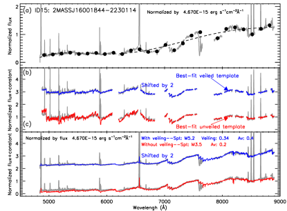
Figure 19: (a) The flux-calibrated spectra of the source 15 normalized by 4.67$\times$10^-15 erg^-1 s^-1 cm^-2 Å^-1. The filled circles mark the wavelength bins used to construct the 5-order polynomial function (the dashed line) to normalize the spectra. (b) The spectra (gray lines) of the source 15 normalized by a 5-order polynomial function overlapped with the best-fit unveiled template and veiled template, which are normalized in the same way as the target’s spectra. (c) The flux-calibrated spectra of the source 15 normalized by 4.67$\times$10^-15 erg^-1 s^-1 cm^-2 Å^-1 overlapped with the best-fit unveiled template and veiled template. The best-fit templates have been flux-calibrated with the Gaia broad-band photometry.

Appendix C Line fluxes and associated uncertainties

We estimate the fluxes of the accretion-related emission lines and the [O I] $\lambda$6300 line using the line $EW$s from fitting the HIRES spectra and the continuum flux near the lines from the flux-calibrated templates. We use two methods to assess the uncertainty in our flux calibration. For the first one, we perform synthetic photometry in the $r$ band from the panstarr survey and the $J$ band from the 2MASS survey. By comparing the synthetic photometry with the observations, we obtain a mean difference of 0.05 dex in the $r$-band flux and 0.04 dex in the $J$-band flux.

Our second method uses the overlapping sample of HIRES and VLT/X-Shooter spectra, a total of 32 sources 31 of which are PDs, and one is a DB. We extract the raw data from ESO archive and obtain the flux-calibrated spectra following the procedure described in Manara et al. (2020). The uncertainty of the flux-calibration is expected to be about $\pm$10% . Fig. 20 compares the 7500 Å fluxes from the X-Shooter and our calibrated spectra. From the comparison, we further estimate the uncertainty on our flux calibration. The mean difference between the two works is about 0.09 dex. Sources 21, 69, and 81 show larger differences (0.24-0.52 dex), which may be attributed to their brightness variability (Cody & Hillenbrand, 2018). If excluding the four outliers in Figure 20, the mean difference between two measurements is reduced to $\sim$0.057 dex. Given that the uncertainty of the flux-calibration on X-Shooter spectra is about $\pm$10%, the comparison suggests that the uncertainty of our absolute flux calibration is likely better than 15%.

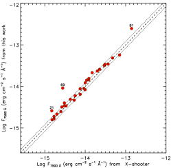
Figure 20: Comparison of 7500 Å fluxes from our work and from X-Shooter spectra. The dash line shows the 1:1 line while dotted lines mark a $\pm$0.08 dex difference.

Appendix D Stellar parameters

We convert the spectral type to the effective temperature using the conversions in Fang et al. (2017), which are from Pecaut & Mamajek (2013) for stars earlier than M4 and from Herczeg & Hillenbrand (2014) for stars later than M4 as the former does not cover all SpTy in our sample while the latter employs a coarse grid for early SpTy. With the effective temperatures, we obtain the stellar luminosity using the flux at 7510 Å from flux-calibrated best-fit templates described in Appendix B and the Bolometric Corrections from Herczeg & Hillenbrand (2014). For the sources with accretion, the flux at 7500 Å only includes the contribution from the stellar photosphere and excludes the excess emission from the accretion shock using the $r_{\rm ex,~{}7500}$ derived from the spectral classification (see § B). The Gaia Data Release 3 geometric distances of individual sources used for computing the stellar luminosity are taken from Bailer-Jones et al. (2021).

Appendix E Spectral energy distributions and [O I] $\lambda$6300 line profiles

Fig. 21 show the SEDs of the sources in this work. Their SEDs are constructed using the the Two-Micron All Sky Survey (2MASS, Skrutskie et al., 2006), the Wide-field Infrared Survey Explorer (WISE, Wright et al., 2010), and the Spitzer photometric data from Esplin et al. (2018). For each source in our sample, we construct a median SED from CTTs with similar spectral type in Orion (Fang et al., 2009, 2013, 2017). In each panel of Figs 21, 22, and  23, we show in red the upper and lower quartiles of the median SEDs, and in gray the upper and lower 42.5% of the median SEDs.

Figures 24, 25, and 26 show the [O I] $\lambda$6300 line profiles for the protoplanetary and debris disks. There are no [O I] $\lambda$6300 detections towards the DBs. For the protoplanetary disks, we divide them into two categories, those with and those without [O I] $\lambda$6300 detection, and show them in separate figures.

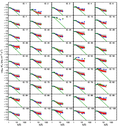
Figure 21: SEDs for the protoplanetary disks with [O I] $\lambda$6300 detection in analyzed our sample in this paper. Filled circles are photometric data from 2MASS and WISE (blue), Spitzer (yellow). The green solid line the stellar photosphere. The grey region shows the upper and lower quarterlies of the Lynds 1641 classical T Tauri median SED. The median SED has been reddened with the extinction of each source, and then normalized to the J-band flux.

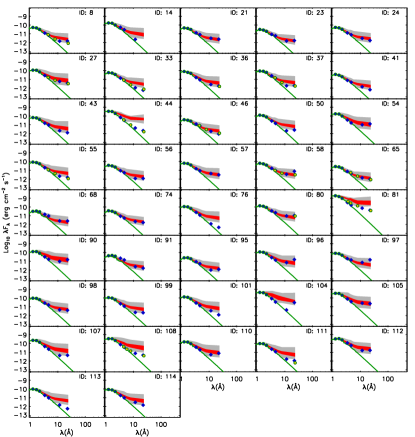
Figure 22: Same as Figure 21 but for the protoplanetary disks without [O I] $\lambda$6300 detection.

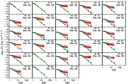
Figure 23: Same as Figure 21 but for sources with debris disks or without disks.

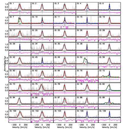
Figure 24: Corrected and uncorrected [O I] $\lambda$6300 line profiles for the protoplanetary disks with [O I] $\lambda$6300 detection in our sample. The figure is same as Fig. 8. The SEDs of the corresponding sources are shown in Fig. 21.

Figure 25: [O I] $\lambda$6300 line profiles for the protoplanetary disks without [O I] $\lambda$6300 detection. The SEDs of the corresponding sources are shown in Fig. 22.

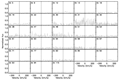
Figure 26: [O I] $\lambda$6300 line profiles for DBs or NDs. The SEDs of the corresponding sources are shown in Fig. 23.

Appendix F The dependence of H$\alpha$ $FW_{\rm H\alpha 10\%}$ on spectral types

We collect a sample of young stars which show accretion activities indicated by the presence of the Balmer continuum excess in their U-band spectra in the literature (Herczeg & Hillenbrand, 2008; Alcalá et al., 2014, 2017; Manara et al., 2016, 2017b; Rugel et al., 2018) and a sample of young stars with debris disks or without disks which show no accretion activities (this work; Jayawardhana et al. 2003; Muzerolle et al. 2005; Jayawardhana et al. 2006; Nguyen et al. 2012).

In Fig. 27, we show the H$\alpha$ $FW_{\rm H\alpha 10\%}$ vs. spectral types for these young stars. Based on it, we propose the thresholds on the H$\alpha$ $FW_{\rm H\alpha 10\%}$ to separate WTTSs from CTTSs within two spectral type ranges. We consider a young star to be a CTTS if H$\alpha$ $FW_{\rm H\alpha 10\%}>250$  km s^-1 for the ones with spectral types earlier than M4 (Fang et al., 2013) and if H$\alpha$ $FW_{\rm H\alpha 10\%}>200$  km s^-1 for later type ones (Jayawardhana et al., 2003). With these criteria, we can separate WTTSs from CTTSs well. However, it is also noted that there are some outliers in Fig. 27. The WTTSs with higher H$\alpha$ $FW_{\rm H\alpha 10\%}$ than the thresholds could be fast rotators or spectroscopic binaries. The CTTSs which show lower H$\alpha$ $FW_{\rm H\alpha 10\%}$ than the thresholds are lower accretors and their H$\alpha$ emissions are dominated by chromospheric emission.

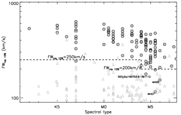
Figure 27: H$\alpha$ $FW_{\rm H\alpha 10\%}$ vs. spectral types for accreting young stars (gray filled circles) and nonaccreting young stars (gray open diamonds). The dashed lines mark the thresholds which classify the CTTS/WTTS within two spectral type bins, earlier than M4 and later than M4.

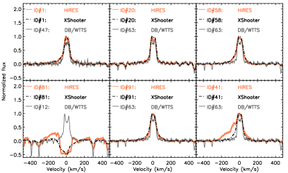
Figure 28: HIRES H$\alpha$ line profiles of 5 WTTSs (ID 1, 20, 58, 81, and 91) and one CTTS (ID 41) classified in this work that have different WTTS/CTTS classification in Manara et al. (2020) based on X-Shooter spectra. As a comparison, for each source we show its X-Shooter H$\alpha$ profile (black) and one H$\alpha$ profile from a DB WTTS (gray) of similar spectral type.

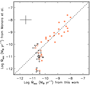
Figure 29: Comparison of accretion rates from this work and from Manara et al. (2020). Left pointing arrows indicate sources classified as WTTSs in this work while downward pointing arrows indicate WTTSs in Manara et al. (2020). The dashed line shows the one-to-one relation. The cross indicates typical uncertainties. The IDs for 5 sources with discrepant WTTS/CTTS classification are marked. ID 81 is not included because there are no accretion-related emission lines in the HIRES spectra. Other symbols are as in Fig. 4.

Appendix G Comparisons of Accretion properties in this work and in the literature

Figure 28 shows the H$\alpha$ profiles of the 6 sources: the HIRES and X-Shooter spectra as well as one H$\alpha$ profile from the DB WTTs with the closest spectral type. We note that for 4 sources (Source 1, 20, 58, and 91) both HIRES and X-Shooter spectra show identical line profiles which are similar to the ones of DB WTTSs, hence our classification as WTTSs. These sources are classified as CTTSs in Manara et al. (2020) but have estimated mass accretion rates below $10^{-10}$ M_⊙ yr^-1  which may be difficult to detect in the H$\alpha$ profiles. For Source 81, both the HIRES and X-Shooter spectra show H$\alpha$ in absorption. On the contrary, for Source 41, the HIRES spectrum clearly shows a blue-shifted broader wing than the X-Shooter one and thus is classified as a CTTS in this work. For this source the discrepancy on the WTTS/CTTS classification might be due to accretion variability.

Figure 29 compares our mass accretion rate estimates with those obtained by Manara et al. (2020) by modeling the Balmer continuum excess for the 32 sources in common with our sample. Note that Source 81 (2MASS J16141107-2305362), which is classified as a CTTS in Manara et al. (2020), does not clearly show any accretion-related emission lines in our HIRES spectra (see Figure 28), hence it is not included in the plot. Manara et al. (2020) report typical uncertainties of 0.36 dex in mass accretion rates which compare well with our overall uncertainty of 0.42 dex . Figure 29 shows an overall good agreement between the two works and the mean difference in the accretion rates of the 21 CTTSs among the two works is 0.38 dex, within the quoted uncertainties.

Thanathibodee et al. (2022) employ a new scheme to classify low accretors based the He I $\lambda$10830 line profile. We collect the X-Shooter spectra for the 32 common young stars from the ESO Phase 3 spectral data archive, and obtain their line profiles of He I $\lambda$10830, see Fig. 30. Thanathibodee et al. (2022) classify the He I $\lambda$10830 line profiles of young stars into six types including Types r, b, br, c, e and f. Type r line profiles show redshifted absorption below the continuum covering velocities comparable to the free-fall velocities, Type b show detectable blueshifted absorption below the continuum, Type bf consist of both blueshifted and redshifted absorption features, Type c show detectable absorption at or near the line center, Type e only show emission features, and Type f are featureless. Thanathibodee et al. (2022) classify the accretion level of young stars using the $\lambda$10830 line profiles: stars are considered to be accreting if their line profiles are types r, b or br, and non accreting if their line profiles are types c, e, or f.

Thanathibodee et al. (2022) have observed a sample of sources in Upper Sco using the FIRE spectrograph at the Magellan Baade Telescope, and among them 22 (see Table 10) are in common with our sample, including 4 (IDs 20, 28, 29, and 49) that are among the above 33 sources. For the 4 sources which have both X-Shooter and FIRE spectra, three (IDs 20, 29, and 49) have the same WTTS/CTTS classification based on the two line profiles of He I $\lambda$10830, and one (ID 28) has different classification which might be due to the accretion variability. If including all the 51 sources with line profiles of He I $\lambda$10830 from either X-Shooter spectra or FIRE spectra, 76% (39/51) of them have same classification in Thanathibodee et al. (2022) and our work. Among the 27 WTTSs classified in this work, 8 sources are classified as CTTSs based on the line profiles of He I $\lambda$10830. In our sample, the fraction (30%, 8/27) of low accretors among WTTSs classifed based on H$\alpha$ line is comparable to the one (27%) for the sources with ages lager than 5 Myr in Thanathibodee et al. (2022). We also note that among the 24 CTTSs classified in this work 5 sources are classified as WTTSs based on the line profiles of He I $\lambda$10830. This might be due these sources having variable accretion. In Table 10, we compare the CTTS/WTTS classification of the Upper Sco sources using different schemes. This comparison further underlines the difficulty in properly classifying low accretors using emission lines.

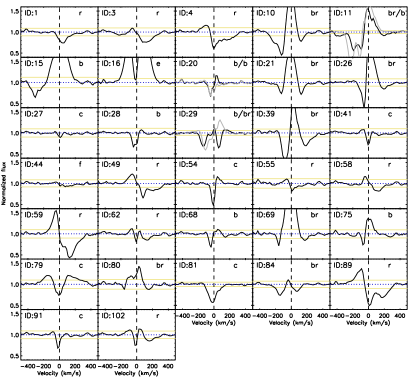
Figure 30: Line profiles of He I $\lambda$10830 for 32 sources with X-Shooter data. The yellow solid lines mark the flux at 3$\sigma$ from the continuum. The features where their extrema above 3$\sigma$ away from the continuum are considered as detections. The type of each profile is shown in each panel. Three sources (IDs 11, 20, and 29) have two X-Shooter spectra. Two of them are shown as comparison.

Appendix H Outliers: WTTS with [O I] $\lambda$6300 detections and CTTS without

Our Upper Sco PD sample includes 13 WTTSs with [O I] $\lambda$6300 detection and 13 CTTSs without [O I] $\lambda$6300 detection. The H$\alpha$ line profiles and [O I] $\lambda$6300 lines of these sources are shown in Figs. 31 and  32. As a comparison, for each source the H$\alpha$ line profiles and [O I] $\lambda$6300 lines of a CTTS and WTTS with similar spectral type are shown.

The [O I] $\lambda$6300 detections in the 13 WTTSs suggest that these sources are still surrounded by a gaseous disk but the H$\alpha$ lines, which are similar to the DB/WTTS, are not sensitive enough to detect small mass accretion rates, see Fig. 31. We note that the [O I] $\lambda$6300 detection rate (33%) among the Upper Sco WTTSs is comparable to the fraction (27%) of low accretors among the sample of the old ($>5$ Myr) WTTSs based on the line profiles of He I $\lambda$10830 (this work and Thanathibodee et al. 2022). This suggests that the [O I] $\lambda$6300 line could be another sensitive tracer of low accretion in addition to the He I $\lambda$10830 line. Indeed, among the 13 WTTSs with the [O I] $\lambda$6300 detections, 9 (Sources 1, 20, 28, 29, 34, 45, 71, 74, and 87) have observed He I $\lambda$10830 line (see Fig. 30 and Thanathibodee et al. 2022) and 5 of them (Sources 1, 20, 28, 29, and 74) have been also classified as low accretors based on the line profiles of He I $\lambda$10830. For the other 4 WTTSs (Sources 34, 45, 71 and 87) which are also classified as nonaccretors based on the line profiles of He I $\lambda$10830 in Thanathibodee et al. (2022), more observations are required to distinguish if they are true nonaccretors or low variable accretors.

The 13 PDs classified as CTTSs but without [O I] $\lambda$6300 detection are shown in Figure 32. These sources have H$\alpha$ profiles with strengths and widths comparable to other CTTSs with spectral types similar to them, but do not shown clear [O I] $\lambda$6300 line. Among them, 6 sources (IDs 21, 41, 44, 56, 69, and 81) have been observed with the He I $\lambda$10830 line, and 4 of them are also classified as accretors based on the line profiles of He I $\lambda$10830. Sources 41 and 44 are classified as a nonaccretor based on the He I $\lambda$10830 line. However, as shown in Fig. 28 for Source 41 this is probably due accretion variability. Source 44 has been classified as a CTTS both in this work and in Manara et al. (2020). As shown in Fig. 9, 5 sources (IDs 8, 21, 41, 56 and 81) have upper limit on their [O I] $\lambda$6300 line luminosity which are one order of magnitude below the expected ones from their accretion luminosity. Banzatti et al. (2019) presented two other young CTTSs, DN Tau and CI Tau, without an [O I] $\lambda$6300 line detection. A comparison with the data in the literature show that for DN Tau its [O I] $\lambda$6300 line was present in 1987 (Hartigan et al., 1995) but disappeared in 2006 (Simon et al., 2016).

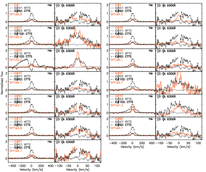
Figure 31: Thirteen WTTSs (orange solid line) with [O I] $\lambda$6300 detection in Upper Sco. For each source, its H$\alpha$ and [O I] $\lambda$6300  line profiles are shown, as well the ones of a CTTS (black dash-dotted line) and WTTS (gray solid line) with the similar spectral type to that source. The line profiles in each panel are normalized by the peak flux of the CTTS line profile.

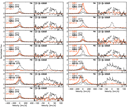
Figure 32: Thirteen CTTSs (orange) without [O I] $\lambda$6300 detection in Upper Sco. In each panel, the lines are same as Fig. 31, beside the orange line is for the CTTS without [O I] $\lambda$6300 detection.

Table 10: A comparison of CTTS/WTTS classification in three schemes

ID	Name	RA	DEC	CTTS				[O I]
				Manara+20	Xshooter HeI	Thanathibodee+22	This work	det
1	2MASSJ15514032-2146103	15 51 40.32	$-$21 46 10.3	Y	Y	$\cdots$	N	Y
3	2MASSJ15530132-2114135	15 53 01.32	$-$21 14 13.5	Y	Y	$\cdots$	Y	Y
4	2MASSJ15534211-2049282	15 53 42.11	$-$20 49 28.2	Y	Y	$\cdots$	Y	Y
10	2MASSJ15582981-2310077	15 58 29.81	$-$23 10 07.7	Y	Y	$\cdots$	Y	Y
11	2MASSJ15583692-2257153	15 58 36.92	$-$22 57 15.3	Y	Y	$\cdots$	Y	Y
15	2MASSJ16001844-2230114	16 00 18.44	$-$22 30 11.4	Y	Y	$\cdots$	Y	Y
16	2MASSJ16014086-2258103	16 01 40.86	$-$22 58 10.3	Y	N	$\cdots$	Y	Y
20	2MASSJ16020757-2257467	16 02 07.57	$-$22 57 46.7	Y	Y	Y	N	Y
21	2MASSJ16024152-2138245	16 02 41.52	$-$21 38 24.5	Y	Y	$\cdots$	Y	N
26	2MASSJ16035767-2031055	16 03 57.67	$-$20 31 05.5	Y	Y	$\cdots$	Y	Y
27	2MASSJ16035793-1942108	16 03 57.93	$-$19 42 10.8	N	N	$\cdots$	N	N
28	2MASSJ16041740-1942287	16 04 17.40	$-$19 42 28.7	N	Y	N	N	Y
29	2MASSJ16042165-2130284	16 04 21.65	$-$21 30 28.4	N	Y	Y	N	Y
39	2MASSJ16062196-1928445	16 06 21.96	$-$19 28 44.5	Y	Y	$\cdots$	Y	Y
41	2MASSJ16063539-2516510	16 06 35.39	$-$25 16 51.0	N	N	$\cdots$	Y	N
44	2MASSJ16064385-1908056	16 06 43.85	$-$19 08 05.6	Y	N	$\cdots$	Y	N
49	2MASSJ16072625-2432079	16 07 26.25	$-$24 32 07.9	Y	Y	Y	Y	Y
54	2MASSJ16081566-2222199	16 08 15.66	$-$22 22 19.9	N	N	$\cdots$	N	N
55	2MASSJ16082751-1949047	16 08 27.51	$-$19 49 04.7	Y	Y	$\cdots$	Y	N
58	2MASSJ16090002-1908368	16 09 00.02	$-$19 08 36.8	Y	Y	$\cdots$	N	N
59	2MASSJ16090075-1908526	16 09 00.75	$-$19 08 52.6	Y	Y	$\cdots$	Y	Y
62	2MASSJ16095361-1754474	16 09 53.61	$-$17 54 47.4	Y	Y	$\cdots$	Y	Y
68	2MASSJ16104636-1840598	16 10 46.36	$-$18 40 59.8	Y	Y	$\cdots$	Y	N
69	2MASSJ16111330-2019029	16 11 13.30	$-$20 19 02.9	Y	Y	$\cdots$	Y	Y
75	2MASSJ16123916-1859284	16 12 39.16	$-$18 59 28.4	Y	Y	$\cdots$	Y	Y
79	2MASSJ16133650-2503473	16 13 36.50	$-$25 03 47.3	Y	N	$\cdots$	Y	Y
80	2MASSJ16135434-2320342	16 13 54.34	$-$23 20 34.2	Y	Y	$\cdots$	Y	N
81	2MASSJ16141107-2305362	16 14 11.07	$-$23 05 36.2	Y	N	$\cdots$	N	N
84	2MASSJ16143367-1900133	16 14 33.67	$-$19 00 13.3	Y	Y	$\cdots$	Y	Y
89	2MASSJ16154416-1921171	16 15 44.16	$-$19 21 17.1	Y	Y	$\cdots$	Y	Y
91	2MASSJ16181904-2028479	16 18 19.04	$-$20 28 47.9	Y	N	$\cdots$	N	N
102	2MASSJ16041893-2430392	16 04 18.93	$-$24 30 39.2	Y	Y	$\cdots$	Y	Y
23	2MASSJ16030161-2207523	16 03 01.61	$-$22 07 52.3	$\cdots$	$\cdots$	Y	N	N
24	2MASSJ16031329-2112569	16 03 13.29	$-$21 12 56.9	$\cdots$	$\cdots$	N	N	N
34	2MASSJ16052661-1957050	16 05 26.61	$-$19 57 05.0	$\cdots$	$\cdots$	N	N	Y
36	2MASSJ16055863-1949029	16 05 58.63	$-$19 49 02.9	$\cdots$	$\cdots$	N	N	N
37	2MASSJ16060061-1957114	16 06 00.61	$-$19 57 11.4	$\cdots$	$\cdots$	N	N	N
42	2MASSJ16064102-2455489	16 06 41.02	$-$24 55 48.9	$\cdots$	$\cdots$	N	Y	Y
43	2MASSJ16064115-2517044	16 06 41.15	$-$25 17 04.4	$\cdots$	$\cdots$	N	N	N
45	2MASSJ16070014-2033092	16 07 00.14	$-$20 33 09.2	$\cdots$	$\cdots$	N	N	Y
50	2MASSJ16072747-2059442	16 07 27.47	$-$20 59 44.2	$\cdots$	$\cdots$	N	N	N
57	2MASSJ16084894-2400045	16 08 48.94	$-$24 00 04.5	$\cdots$	$\cdots$	N	N	N
70	2MASSJ16111534-1757214	16 11 15.34	$-$17 57 21.4	$\cdots$	$\cdots$	N	N	Y
73	2MASSJ16115091-2012098	16 11 50.91	$-$20 12 09.8	$\cdots$	$\cdots$	Y	N	Y
74	2MASSJ16122737-2009596	16 12 27.37	$-$20 09 59.6	$\cdots$	$\cdots$	Y	N	N
86	2MASSJ16145928-2459308	16 14 59.28	$-$24 59 30.8	$\cdots$	$\cdots$	N	N	Y
90	2MASSJ16163345-2521505	16 16 33.45	$-$25 21 50.5	$\cdots$	$\cdots$	N	N	N
101	2MASSJ16023587-2320170	16 02 35.87	$-$23 20 17.0	$\cdots$	$\cdots$	N	N	N
105	2MASSJ16093164-2229224	16 09 31.64	$-$22 29 22.4	$\cdots$	$\cdots$	N	N	N
111	2MASSJ16145244-2513523	16 14 52.44	$-$25 13 52.3	$\cdots$	$\cdots$	N	N	N

References

- Alcalá et al. (2014) Alcalá, J. M., Natta, A., Manara, C. F., et al. 2014, A&A, 561, A2
- Alcalá et al. (2017) Alcalá, J. M., Manara, C. F., Natta, A., et al. 2017, A&A, 600, A20
- Alexander et al. (2014) Alexander, R., Pascucci, I., Andrews, S., Armitage, P., & Cieza, L. 2014, in Protostars and Planets VI, ed. H. Beuther, R. S. Klessen, C. P. Dullemond, & T. Henning, 475
- Ansdell et al. (2016) Ansdell, M., Williams, J. P., van der Marel, N., et al. 2016, ApJ, 828, 46
- Bacciotti et al. (2000) Bacciotti, F., Mundt, R., Ray, T. P., et al. 2000, ApJ, 537, L49
- Bai (2016) Bai, X.-N. 2016, ApJ, 821, 80
- Bailer-Jones et al. (2021) Bailer-Jones, C. A. L., Rybizki, J., Fouesneau, M., Demleitner, M., & Andrae, R. 2021, AJ, 161, 147
- Banzatti et al. (2019) Banzatti, A., Pascucci, I., Edwards, S., et al. 2019, ApJ, 870, 76
- Barenfeld et al. (2016) Barenfeld, S. A., Carpenter, J. M., Ricci, L., & Isella, A. 2016, ApJ, 827, 142
- Barenfeld et al. (2017) Barenfeld, S. A., Carpenter, J. M., Sargent, A. I., Isella, A., & Ricci, L. 2017, ApJ, 851, 85
- Barrado y Navascués & Martín (2003) Barrado y Navascués, D., & Martín, E. L. 2003, AJ, 126, 2997
- Béthune et al. (2017) Béthune, W., Lesur, G., & Ferreira, J. 2017, A&A, 600, A75
- Cardelli et al. (1989) Cardelli, J. A., Clayton, G. C., & Mathis, J. S. 1989, ApJ, 345, 245
- Carpenter et al. (2006) Carpenter, J. M., Mamajek, E. E., Hillenbrand, L. A., & Meyer, M. R. 2006, ApJ, 651, L49
- Cody & Hillenbrand (2018) Cody, A. M., & Hillenbrand, L. A. 2018, AJ, 156, 71
- Cutri et al. (2021) Cutri, R. M., Wright, E. L., Conrow, T., et al. 2021, VizieR Online Data Catalog, II/328
- David et al. (2019a) David, T. J., Hillenbrand, L. A., Gillen, E., et al. 2019a, ApJ, 872, 161
- David et al. (2019b) —. 2019b, ApJ, 872, 161
- Dong et al. (2017) Dong, R., van der Marel, N., Hashimoto, J., et al. 2017, ApJ, 836, 201
- Edwards et al. (1987) Edwards, S., Cabrit, S., Strom, S. E., et al. 1987, ApJ, 321, 473
- Espaillat et al. (2014) Espaillat, C., Muzerolle, J., Najita, J., et al. 2014, in Protostars and Planets VI, ed. H. Beuther, R. S. Klessen, C. P. Dullemond, & T. Henning, 497
- Esplin et al. (2018) Esplin, T. L., Luhman, K. L., Miller, E. B., & Mamajek, E. E. 2018, AJ, 156, 75
- Fang et al. (2021) Fang, M., Kim, J. S., Pascucci, I., & Apai, D. 2021, ApJ, 908, 49
- Fang et al. (2013) Fang, M., Kim, J. S., van Boekel, R., et al. 2013, ApJS, 207, 5
- Fang et al. (2009) Fang, M., van Boekel, R., Wang, W., et al. 2009, A&A, 504, 461
- Fang et al. (2017) Fang, M., Kim, J. S., Pascucci, I., et al. 2017, AJ, 153, 188
- Fang et al. (2018) Fang, M., Pascucci, I., Edwards, S., et al. 2018, ApJ, 868, 28
- Feiden (2016) Feiden, G. A. 2016, A&A, 593, A99
- Frank et al. (2014) Frank, A., Ray, T. P., Cabrit, S., et al. 2014, Protostars and Planets VI, 451
- Furlan et al. (2009) Furlan, E., Watson, D. M., McClure, M. K., et al. 2009, ApJ, 703, 1964
- Gorti et al. (2016) Gorti, U., Liseau, R., Sándor, Z., & Clarke, C. 2016, Space Sci. Rev., 205, 125
- Green et al. (2019) Green, G. M., Schlafly, E., Zucker, C., Speagle, J. S., & Finkbeiner, D. 2019, ApJ, 887, 93
- Gressel et al. (2015) Gressel, O., Turner, N. J., Nelson, R. P., & McNally, C. P. 2015, ApJ, 801, 84
- Gullbring et al. (1998) Gullbring, E., Hartmann, L., Briceno, C., & Calvet, N. 1998, ApJ, 492, 323
- Hartigan et al. (1995) Hartigan, P., Edwards, S., & Ghandour, L. 1995, ApJ, 452, 736
- Hartigan et al. (1989) Hartigan, P., Hartmann, L., Kenyon, S., Hewett, R., & Stauffer, J. 1989, ApJS, 70, 899
- Hartmann et al. (2016) Hartmann, L., Herczeg, G., & Calvet, N. 2016, ARA&A, 54, 135
- Herczeg & Hillenbrand (2008) Herczeg, G. J., & Hillenbrand, L. A. 2008, ApJ, 681, 594
- Herczeg & Hillenbrand (2014) —. 2014, ApJ, 786, 97
- Hughes et al. (2010) Hughes, A. M., Andrews, S. M., Wilner, D. J., et al. 2010, AJ, 140, 887
- Husser et al. (2013) Husser, T.-O., Wende-von Berg, S., Dreizler, S., et al. 2013, A&A, 553, A6
- Jayawardhana et al. (2006) Jayawardhana, R., Coffey, J., Scholz, A., Brandeker, A., & van Kerkwijk, M. H. 2006, ApJ, 648, 1206
- Jayawardhana et al. (2003) Jayawardhana, R., Mohanty, S., & Basri, G. 2003, ApJ, 592, 282
- Kwan & Tademaru (1995) Kwan, J., & Tademaru, E. 1995, ApJ, 454, 382
- Lavalley-Fouquet et al. (2000) Lavalley-Fouquet, C., Cabrit, S., & Dougados, C. 2000, A&A, 356, L41
- Lesur et al. (2022) Lesur, G., Ercolano, B., Flock, M., et al. 2022, arXiv e-prints, arXiv:2203.09821
- Luhman (1999) Luhman, K. L. 1999, ApJ, 525, 466
- Luhman (2004) —. 2004, ApJ, 617, 1216
- Luhman (2006) —. 2006, ApJ, 645, 676
- Luhman (2022) —. 2022, AJ, 163, 25
- Luhman & Mamajek (2012) Luhman, K. L., & Mamajek, E. E. 2012, ApJ, 758, 31
- Luhman et al. (2003) Luhman, K. L., Stauffer, J. R., Muench, A. A., et al. 2003, ApJ, 593, 1093
- MacGregor et al. (2017) MacGregor, M. A., Wilner, D. J., Czekala, I., et al. 2017, ApJ, 835, 17
- Manara et al. (2016) Manara, C. F., Fedele, D., Herczeg, G. J., & Teixeira, P. S. 2016, A&A, 585, A136
- Manara et al. (2017a) Manara, C. F., Frasca, A., Alcalá, J. M., et al. 2017a, A&A, 605, A86
- Manara et al. (2013) Manara, C. F., Testi, L., Rigliaco, E., et al. 2013, A&A, 551, A107
- Manara et al. (2017b) Manara, C. F., Testi, L., Herczeg, G. J., et al. 2017b, A&A, 604, A127
- Manara et al. (2020) Manara, C. F., Natta, A., Rosotti, G. P., et al. 2020, A&A, 639, A58
- McGinnis et al. (2018) McGinnis, P., Dougados, C., Alencar, S. H. P., Bouvier, J., & Cabrit, S. 2018, A&A, 620, A87
- Mészáros et al. (2012) Mészáros, S., Allende Prieto, C., Edvardsson, B., et al. 2012, AJ, 144, 120
- Muzerolle et al. (2005) Muzerolle, J., Luhman, K. L., Briceño, C., Hartmann, L., & Calvet, N. 2005, ApJ, 625, 906
- Natta et al. (2014) Natta, A., Testi, L., Alcalá, J. M., et al. 2014, A&A, 569, A5
- Natta et al. (2004) Natta, A., Testi, L., Muzerolle, J., et al. 2004, A&A, 424, 603
- Nguyen et al. (2012) Nguyen, D. C., Brandeker, A., van Kerkwijk, M. H., & Jayawardhana, R. 2012, ApJ, 745, 119
- Nisini et al. (2018) Nisini, B., Antoniucci, S., Alcalá, J. M., et al. 2018, A&A, 609, A87
- Pascucci et al. (2022) Pascucci, I., Cabrit, S., Edwards, S., et al. 2022, arXiv e-prints, arXiv:2203.10068
- Pascucci et al. (2015) Pascucci, I., Edwards, S., Heyer, M., et al. 2015, ApJ, 814, 14
- Pascucci et al. (2020) Pascucci, I., Banzatti, A., Gorti, U., et al. 2020, ApJ, 903, 78
- Pecaut & Mamajek (2013) Pecaut, M. J., & Mamajek, E. E. 2013, ApJS, 208, 9
- Pecaut et al. (2012) Pecaut, M. J., Mamajek, E. E., & Bubar, E. J. 2012, ApJ, 746, 154
- Pinte et al. (2022) Pinte, C., Teague, R., Flaherty, K., et al. 2022, arXiv e-prints, arXiv:2203.09528
- Pontoppidan et al. (2011) Pontoppidan, K. M., Blake, G. A., & Smette, A. 2011, ApJ, 733, 84
- Pudritz & Ray (2019) Pudritz, R. E., & Ray, T. P. 2019, Frontiers in Astronomy and Space Sciences, 6, 54
- Rigliaco et al. (2012) Rigliaco, E., Natta, A., Testi, L., et al. 2012, A&A, 548, A56
- Rigliaco et al. (2013) Rigliaco, E., Pascucci, I., Gorti, U., Edwards, S., & Hollenbach, D. 2013, ApJ, 772, 60
- Rugel et al. (2018) Rugel, M., Fedele, D., & Herczeg, G. 2018, A&A, 609, A70
- Simon et al. (2017) Simon, M., Guilloteau, S., Di Folco, E., et al. 2017, ApJ, 844, 158
- Simon et al. (2016) Simon, M. N., Pascucci, I., Edwards, S., et al. 2016, ApJ, 831, 169
- Skrutskie et al. (2006) Skrutskie, M. F., Cutri, R. M., Stiening, R., et al. 2006, AJ, 131, 1163
- Sung et al. (2009) Sung, H., Stauffer, J. R., & Bessell, M. S. 2009, AJ, 138, 1116
- Tazzari et al. (2017) Tazzari, M., Testi, L., Natta, A., et al. 2017, A&A, 606, A88