On the stability properties of power networks with time-varying inertia

Abstract

A major transition in modern power systems is the replacement of conventional generation units with renewable sources of energy. The latter results in lower rotational inertia which compromises the stability of the power system, as testified by the growing number of frequency incidents. To resolve this problem, numerous studies have proposed the use of virtual inertia to improve the stability properties of the power grid. In this study, we consider how inertia variations, resulting from the application of control action associated with virtual inertia and fluctuations in renewable generation, may affect the stability properties of the power network within the primary frequency control timeframe. We consider the interaction between the frequency dynamics and a broad class of power supply dynamics in the presence of time-varying inertia and provide locally verifiable conditions, that enable scalable designs, such that stability is guaranteed. To complement the presented stability analysis and highlight the dangers arising from varying inertia, we provide analytic conditions that enable to deduce instability from single-bus inertia fluctuations. Our analytical results are validated with simulations on the Northeast Power Coordinating Council (NPCC) 140-bus system, where we demonstrate how inertia variations may induce large frequency oscillations and show that the application of the proposed conditions yields a stable response.

I Introduction

Motivation and literature review: The electric power grid is currently undergoing through a major transformation due to the growing penetration of renewable sources of energy [2], [3]. As a result, conventional bulk generation is expected to be slowly replaced by renewable generation. However, retiring synchronous generation lowers the rotational inertia of the power system, which has been a key reason for the power grid’s stability over the years [4]. In addition, renewable generation is intermittent, causing more frequent generation-demand imbalances that may harm the power quality and even cause blackouts [5]. Hence, novel challenges are introduced towards enabling a stable and robust operation of the power grid.

The inertia of the power system represents its capability to store and inject kinetic energy, serving as an energy buffer that can slow down the frequency dynamics. The latter aids to effectively avoid undesirable incidents, such as excessive load-shedding or large-scale blackouts. A low power system inertia is associated with larger frequency deviations following a disturbance event, such as loss of generation or tie line faults [6]. The degrading effects of low inertia levels on the power system stability have already been reported by system operators [7]. To mitigate these effects, several studies proposed the introduction of virtual inertia in the power grid, i.e. schemes that aim to resemble the inertial response of machines by injecting power in proportion to the rate of change of frequency. In particular, [8] proposed the use of the energy stored in the DC-link capacitors of grid-connected power converters to emulate the inertia of the power system. Control schemes of varying complexity that aim to make converters behave in a similar way as synchronous machines and provide virtual inertia to the power grid have been investigated in [9], [10], [11], [12], [13]. These schemes require some form of energy storage, such as batteries, to provide the required energy. In addition, [14] proposed the integration of DC microgrids into the power network as virtual synchronous machines (VSMs). Moreover, [15] designed a self tuning mechanism to optimize the operation of VSMs. The scheme proposed in [16] uses the kinetic energy stored in the rotating mass of wind turbine blades to emulate inertia and provide frequency support. Furthermore, [17], [18] demonstrated how power converters can mimic the inertial response of a synchronous machine for wind turbines interconnected to the grid via doubly fed induction generators. The optimal placement of virtual inertia is considered in [19]. Comprehensive reviews on virtual inertia and virtual synchronous machine schemes are available in [20] and [21] respectively.

An open research question that requires further attention concerns the effect of varying inertia on the stability properties of the power network. Variations in inertia may arise due to fluctuations in renewable generation and control action on virtual inertia. Controllable virtual inertia, possibly coupled with the power grid dynamics, may induce additional challenges for the stability of the power grid. In addition, it may pose security threats, if inertia is maliciously controlled to destabilize the power grid. The time-varying nature of inertia has been pointed out and studied in [6]. In addition, [22] considered the robustness properties of power networks with time-varying inertia and frequency damping, while [23] considered a hybrid model of the power network with time-varying inertia and applied model predictive control approaches to optimize the power inputs. In [24], the authors considered the effect of inertia variations in the frequency response. Stabilizing controllers under various inertia modes are designed in [25] using a linear quadratic regulator approach. Furthermore, [26] and [27] proposed time-varying control gains associated with the inertia and damping of wind turbines and the inertia of virtual synchronous generators respectively. However, a systematic approach on how time-varying inertia affects the stability properties of power networks is currently missing from the literature. This may lead to suitable guidelines for the design of virtual inertia schemes that offer improved stability and security properties.

Contribution: This study investigates the impact of time-varying inertia on the behaviour and stability properties of the power network within the primary frequency control timeframe. In particular, we consider the interaction between the frequency dynamics and non-linear power supply dynamics in the presence of time-varying inertia. We study the solutions of this time-varying system and analytically deduce local asymptotic stability under two proposed conditions. The first condition, inspired from [28], requires that the aggregate power supply dynamics at each bus satisfy a passivity related property. The second condition sets a bound on the maximum rate of growth of inertia that depends on the local power supply dynamics. Both conditions are locally verifiable and applicable to general network topologies and enable practical guidelines for the design of virtual inertia control schemes that enhance the reliability and security of the power network.

To demonstrate the applicability and improve the intuition on the proposed analysis, we provide examples of power supply dynamics that fit within the presented framework and explain how the maximum allowable rate of inertia variation may be deduced for these cases. In addition, when linear power supply dynamics are considered, we show how the conditions can be efficiently verified by solving a suitable linear matrix inequality optimization problem.

Our stability results are complemented by analytical results that demonstrate how single-bus inertia variations may induce unstable behaviour. In particular, we provide conditions such that for any, arbitrarily small, deviation from the equilibrium frequency at a single bus, there exist local inertia trajectories that result in substantial deviations in the power network frequency. The latter coincides with the definition of instability (e.g. [29, Dfn. 4.1]).

Numerical simulations on the NPCC 140-bus system demonstrate the potentially destabilizing effects of varying inertia and validate our analytical results on a realistic setting. In particular, we demonstrate how varying virtual inertia, at a single or multiple buses, may induce large frequency oscillations and compromise the stability of the power network. The latter provides further motivation for the study and regulation of virtual inertia schemes. In addition, we present how the application of the proposed conditions yields a stable response.

To the authors best knowledge, this is the first work that:

1. Analytically studies the behaviour of power networks under varying inertia and proposes decentralized conditions on the local power supply dynamics and inertia trajectories such that stability is guaranteed.

2. Demonstrates, under broadly applicable conditions, that single-bus inertia variations may induce large frequency fluctuations from any, arbitrarily small, frequency deviation from the equilibrium. Such behaviour is characterized as unstable.

Paper structure: In Section II we present the power network model, a general description for the power supply dynamics and a statement of the problem that we consider. In Section III we present our proposed conditions on the power supply dynamics. Section IV contains the conditions on virtual inertia trajectories and the main result associated with the stability of the power network. In addition, in Section V we provide additional intuition on the stability result and discuss various application examples. Moreover, in Section VI we present our inertia induced instability analysis. Our analytical results are verified with numerical simulations in Section VII and conclusions are drawn in Section VIII. Proofs of the main results are provided in the appendix.

Notation: Real, positive real, integer and positive natural numbers are denoted by $\mathbb{R},\mathbb{R}_{+},\mathbb{Z}$ and $\mathbb{N}_{+}$ respectively. The set of n-dimensional vectors with real entries is denoted by $\mathbb{R}^{n}$. For $a\in\mathbb{R},b\in\mathbb{R}\setminus\{0\}$, $a$ modulo $b$ is denoted by $\mathrm{mod}(a,b)$ and defined as $\mathrm{mod}(a,b)=a-b\lfloor\frac{a}{b}\rfloor$, where for $x\in\mathbb{R}$, $\lfloor x\rfloor=\sup\{m\in\mathbb{Z}:m\leq x\}$. The $p$-norm of a vector $x\in\mathbb{R}^{n}$ is given by $\left\lVert x\right\rVert_{p}=(|x_{1}|^{p}+\dots+|x_{n}|^{p})^{1/p},1\leq p<\infty$. A function $f:\mathbb{R}^{n}\rightarrow\mathbb{R}^{m}$ is said to be locally Lipschitz continuous at $x$ if there exists some neighbourhood $X$ of $x$ and some constant $L$ such that $\left\lVert f(x)-f(y)\right\rVert\leq L\left\lVert x-y\right\rVert$ for all $y\in X$, where $\left\lVert.\right\rVert$ denotes any $p$-norm. The Laplace transformation of a signal $x(t),x:\mathbb{R}\rightarrow\mathbb{R}$, is denoted by $\hat{x}(s)=\int_{0}^{\infty}x(t)e^{-st}dt$. A function $f:\mathbb{R}^{n}\rightarrow\mathbb{R}$ is called positive semidefinite if $f(x)\geq 0$ for all $x\in\mathbb{R}^{n}$. The function sin$(x)$ gives the sinusoid of each element in $x\in\mathbb{R}^{n}$, i.e. for $x=[x_{1}\;x_{2}\dots x_{n}]^{T}$, sin$(x)=[\sin(x_{1})\;\sin(x_{2})\dots\sin(x_{n})]^{T}$. For a matrix $A\in\mathbb{R}^{n\times p}$, $A_{kl}$ corresponds to the element in the $k$th row and $l$th column of $A$. A matrix $A\in\mathbb{R}^{n\times n}$ is called diagonal if $A_{ij}=0$ for all $i\neq j$ and positive (negative) semi-definite, symbolized with $A\succeq 0$ (respectively $A\preceq 0)$, if $x^{T}Ax\geq 0$ (respectively $x^{T}Ax\leq 0$) for all $x\in\mathbb{R}^{n}$. For $a\in~{}\mathbb{R}^{n},b\in~{}\mathbb{R}_{+}$, the ball $\mathcal{B}(a,b)$ is defined as $\mathcal{B}(a,b)=\{x:\left\lVert a-x\right\rVert\leq b\}$. Finally, for a state $x\in\mathbb{R}^{n}$, we let $x^{*}$ denote its equilibrium value.

II Problem formulation

II-A Network model

We describe the power network by a connected graph $(\mathcal{N},\mathcal{E})$ where $\mathcal{N}=\{1,2,\dots,|\mathcal{N}|\}$ is the set of buses and $\mathcal{E}\subseteq\mathcal{N}\times\mathcal{N}$ the set of transmission lines connecting the buses. Furthermore, we use $(k,l)$ to denote the link connecting buses $k$ and $l$ and assume that the graph $(\mathcal{N},\mathcal{E})$ is directed with an arbitrary orientation, so that if $(k,l)\in\mathcal{E}$ then $(l,k)\notin\mathcal{E}$. For each $j\in\mathcal{N}$, we define the sets of predecessor and successor buses by $\mathcal{N}^{p}_{j}=\{k:(k,j)\in\mathcal{E}\}$ and $\mathcal{N}^{s}_{j}=\{k:(j,k)\in\mathcal{E}\}$ respectively. The structure of the network can be represented by its incidence matrix $H\in\mathbb{R}^{|\mathcal{N}|\times|\mathcal{E}|}$, defined as

$$H_{kq}=\begin{cases}+1,\text{ if }k\text{ is the positive end of edge }q,\\ -1,\text{ if }k\text{ is the negative end of edge }q,\\ 0,\text{ otherwise.}\end{cases}$$

It should be noted that any change in the graph ordering does not alter the form of the considered dynamics. In addition, all the results presented in this paper are independent of the choice of graph ordering. We consider the following conditions for the power network:
1) Bus voltage magnitudes are $|V_{j}|=1$ per unit for all $j\in\mathcal{N}$.
2) Lines $(k,l)\in\mathcal{E}$ are lossless and characterized by the magnitudes of their susceptances $B_{kl}=B_{lk}>0$.
3) Reactive power flows do not affect bus voltage phase angles and frequencies.
These conditions have been widely used in the literature in studies associated with frequency regulation, e.g. [23], [28], [30], [31]. In practice, they are valid in medium to high voltage transmission systems since transmission lines are dominantly inductive and voltage variations are small. It should be noted that all results presented in this paper are verified with numerical simulations, presented in Section VII, on a more detailed model than our analytical one which includes voltage dynamics, line resistances and reactive power flows.

We use the swing equations to describe the rate of change of frequency at each bus. This motivates the following system dynamics (e.g. [32]),

$$\dot{\eta}_{kl}=\omega_{k}-\omega_{l},\;(k,l)\in\mathcal{E},$$ (1a)

$$M^{0}_{j}\dot{\omega}_{j}=-p_{j}^{L}+p_{j}^{M}-d^{c}_{j}-d^{u}_{j}+p^{v}_{j}-\sum_{k\in\mathcal{N}^{s}_{j}}p_{jk}+\sum_{l\in\mathcal{N}^{p}_{j}}p_{lj},j\in\mathcal{N},$$ (1b)

$$p_{kl}=B_{kl}\sin\eta_{kl},\;(k,l)\in\mathcal{E}.$$ (1c)

In system (1), variables $p^{M}_{j}$ and $\omega_{j}$ represent, respectively, the mechanical power injection and the deviation from the nominal value of the frequency at bus $j$. Variables $d^{c}_{j}$ and $d^{u}_{j}$ represent the controllable demand and the uncontrollable frequency-dependent load and generation damping present at bus $j$ respectively. Furthermore, variables $\eta_{kl}$ and $p_{kl}$ represent, respectively, the power angle difference and the power transmitted from bus $k$ to bus $l$. The positive constant $M^{0}_{j}$ denotes the physical inertia at bus $j$. Moreover, the constant $p^{L}_{j}$ denotes the frequency-independent load at bus $j$. Finally, the variable $p^{v}_{j}$ denotes the power injection at bus $j$ associated with time-varying inertia at bus $j$. Its dynamics follow the virtual inertia schemes presented in e.g. [15], [21], [26],

$$p^{v}_{j}=-M^{v}_{j}\dot{\omega}_{j}-D^{v}_{j}\omega_{j},j\in\mathcal{N},$$ (2)

but with a time-varying value of the virtual inertia $M^{v}_{j}$. In particular, in (2), $M^{v}_{j}$ is a non-negative time-dependent variable describing the time-varying virtual inertia at bus $j$ and the constant $D^{v}_{j}\geq 0$ corresponds to the frequency damping coefficient associated with $p^{v}_{j}$.

Remark 1

We have opted to consider a constant rather than a time-varying damping coefficient $D^{v}_{j}$ in (2). This choice is made for simplicity and to keep the focus of the paper on the time-varying inertia. Including time-varying damping coefficients would result in non-existence of equilibria in primary frequency control since these characterize the equilibrium frequency. Jointly considering both time-varying inertia and time-varying damping coefficients is an interesting research problem for future work.

It will be convenient to define the time-varying parameters $M_{j}=M^{0}_{j}+M^{v}_{j}$ describing the aggregate inertia at bus $j$. In addition, we consider the net supply variables $s_{j}$, defined as the aggregation of the mechanical power supply, the controllable demand, the uncontrollable frequency-dependent load and the generation and virtual inertia damping present at bus $j$, as given below

$$s_{j}=p^{M}_{j}-d^{c}_{j}-d^{u}_{j}-D^{v}_{j}\omega_{j},\;j\in\mathcal{N}.$$ (3)

The above enable to compactly represent (1)-(3) by

$$\dot{\eta} =H^{T}\omega,$$ (4a)

$$M\dot{\omega} =-p^{L}+s-Hp,$$ (4b)

$$p =B\text{ {sin}}(\eta),$$ (4c)

where $\eta,p\in\mathbb{R}^{|\mathcal{E}|}$ and $\omega,s,p^{L}\in\mathbb{R}^{|\mathcal{N}|}$ are vectors associated with variables $\eta_{kl},p_{kl},(k,l)\in\mathcal{E}$ and $\omega_{j},s_{j},p^{L}_{j},j\in\mathcal{N}$ respectively. Furthermore, $M\in\mathbb{R}^{|\mathcal{N}|\times|\mathcal{N}|}$ and $B\in\mathbb{R}^{|\mathcal{E}|\times|\mathcal{E}|}$ are diagonal matrices containing the variables $M_{j},j\in\mathcal{N}$ and parameters $B_{kl},(k,l)\in\mathcal{E}$.

II-B Power supply dynamics

To investigate a broad class of power supply dynamics, we will consider the following general dynamic description

$$\begin{aligned} &\dot{x}^{s}_{j}=f_{j}(x^{s}_{j},-\omega_{j}),\\ &s_{j}=g_{j}(x^{s}_{j},-\omega_{j}),\end{aligned}\hskip 7.11317ptj\in\mathcal{N},$$ (5)

where $x^{s}_{j}\in\mathbb{R}^{n_{j}}$ denotes the internal states of the power supply variables, used to update the outputs $s_{j},j\in\mathcal{N}$. In addition, we assume that the maps $f_{j}:\mathbb{R}^{n_{j}}\times\mathbb{R}\to\mathbb{R}^{n_{j}}$ and $g_{j}:\mathbb{R}^{n_{j}}\times\mathbb{R}\to\mathbb{R}$ for all $j\in\mathcal{N}$ are locally Lipschitz continuous. Moreover, we assume that in (5), for any constant input $\omega_{j}(t)=\bar{\omega}_{j}$, there exists a unique locally asymptotically stable equilibrium point $\bar{x}^{s}_{j}\in\mathbb{R}^{n_{j}}$, i.e. satisfying $f_{j}(\bar{x}^{s}_{j},-\bar{\omega}_{j})=0$. The region of attraction of $\bar{x}^{s}_{j}$ is denoted by $\Psi_{j}$. To facilitate the characterization of the equilibria, we also define the static input-state characteristic map $k_{x,j}:\mathbb{R}\to\mathbb{R}^{n_{j}}$ as $k_{x,j}(-\bar{\omega}_{j}):=\bar{x}^{s}_{j},j\in\mathcal{N},$ such that $f_{j}(k_{x,j}(-\bar{\omega}_{j}),-\bar{\omega}_{j})=0$.

It should be noted that the dynamics in (5) are decentralized, depending only on the local frequency $\omega_{j}$ for each $j\in\mathcal{N}$. For notational convenience, we collect the variables in (5) into the vector $x^{s}=[x{{}^{s}_{j}}]_{j\in\mathcal{N}}$.

Remark 2

The power supply variables represent the aggregation of the mechanical generation, controllable demand and uncontrollable frequency dependent demand and frequency damping, as follows from (3). Each of these quantities includes its own dynamics and could be represented in analogy to (5). We opted to consider a combined representation of these quantities for simplicity in presentation. However, the results presented in the paper can be trivially extended to the case where these quantities are described as individual dynamical systems.

II-C Problem statement

This study aims to provide local analytic conditions that associate the inertia variations and power supply dynamics such that stability is guaranteed. The problem is stated as follows.

Problem 1

Provide conditions on the time-varying inertia and power supply dynamics associated with (4)–(5) that:

1. Enable asymptotic stability guarantees.

2. Are locally verifiable.

3. Apply to high order and nonlinear power supply dynamics.

4. Are independent of the (connected) network topology.

The first aim requires conditions that enable asymptotic stability guarantees for the power system. The second objective requires conditions that can be verified using local information, enabling plug-and-play designs. In addition, to enhance the practicality of our results, it is desired that those include a broad range of power supply dynamics, including high order and nonlinear dynamics. Lastly, we aim for conditions that are applicable to general network topologies, i.e. that do not rely on the power network structure, to enable scalable designs.

III Conditions on power supply dynamics

In this section we study the equilibria of (4)–(5) and provide analytic conditions on the power supply dynamics that are subsequently used to solve Problem 1.

III-A Equilibrium analysis

We now define the equilibria of the system (4)–(5).

Definition 1

The constants $(\eta^{*},\omega^{*},x^{s,*})$ define an equilibrium of the system (4)–(5) if the following hold

$$0 =H^{T}\omega^{*},$$ (6a)

$$0 =-p^{L}+s^{*}-Hp^{*},$$ (6b)

$$x^{s,*}_{j} =k_{x,j}(-\omega^{*}_{j}),\;j\in\mathcal{N},$$ (6c)

where $$p^{*} s^{*}$$ and in (6b) are given by

$$\hskip 19.91692ptp^{*} =B\text{ {sin}}(\eta^{*}),$$ (6d)

$$s^{*}_{j} =g_{j}(x^{s,*}_{j},-\omega^{*}_{j}),\;j\in\mathcal{N}.$$ (6e)

For compactness in presentation, we let $\beta=(\eta,\omega,x^{s})$ where $\beta\in\mathbb{R}^{m},m=|\mathcal{E}|+|\mathcal{N}|+\sum_{j\in\mathcal{N}}n_{j}$.

Remark 3

The equilibrium frequency $\omega^{*}$ uniquely defines the values of $x^{s,*}$ and $s^{*}$ due to the uniqueness property of the static input-state maps $k_{x,j},j\in\mathcal{N}$ described in Section II-B. By contrast, the equilibrium values of $\eta^{*}$ and correspondingly $p^{*}$ are not, in general, unique. However, these are unique under specific network configurations, such as in tree networks.

Remark 4

It should be noted that the time-dependent inertia $M_{j},j\in\mathcal{N},$ does not appear in the equilibrium conditions. The latter follows directly from (4b), i.e. the inertia affects the rate of change of frequency but not its equilibrium value. However, as shall be discussed in the following sections, the inertia trajectories have significant impact on whether the system will converge to an equilibrium; i.e., they determine the stability properties of the equilibria.

It should be noted that it trivially follows from (6a) that the equilibrium frequencies of (5), (11) synchronize, i.e. they satisfy $\omega^{*}_{i}=\omega^{*}_{j}=\omega^{s,\ast},\forall i,j\in\mathcal{N}$, where $\omega^{s,\ast}\in\mathbb{R}$ denotes their common value.

For the remainder of the paper we assume the existence of some equilibrium to (4)–(5) following Definition 1. Any such equilibrium is described by $\beta^{*}=(\eta^{*},\omega^{*},x^{s,*})$. Furthermore, we make the following assumption on the equilibrium power angle differences.

Assumption 1

$|\eta^{*}_{ij}|<\tfrac{\pi}{2}$ for all $(i,j)\in\mathcal{E}$.

The condition imposed by Assumption 1 can be interpreted as a security constraint that enables to deduce local convergence. In addition, it is associated with the existence of a synchronizing frequency (see [33]).

III-B Passivity conditions on power supply dynamics

In this section we impose conditions on the power supply dynamics which will be used to prove our main convergence result in Section IV. In particular, we introduce the following passivity notion for dynamics described by (5).

Definition 2

System (5) is said to be locally input strictly passive with strictness constant $\rho_{j}$ about the constant input value $-\bar{\omega}_{j}$ and the constant state values $\bar{x}^{s}_{j}$, if there exist open neighbourhoods $\Omega_{j}$ of $\bar{\omega}_{j}$ and $X_{j}$ of $\bar{x}^{s}_{j}$ and a continuously differentiable, positive semidefinite function $V_{j}(x^{s}_{j})$ (the storage function), with a strict local minimum at $x^{s}_{j}=\bar{x}^{s}_{j}$, such that for all $\omega_{j}\in\Omega_{j}$ and all $x^{s}_{j}\in X_{j}$,

$$\dot{V}_{j}\leq(-\omega_{j}-(-\bar{\omega}_{j}))(s_{j}-\bar{s}_{j})-\rho_{j}(-\omega_{j}-(-\bar{\omega}_{j}))^{2},$$

where $\rho_{j}>0$ and $\bar{s}_{j}=g_{j}(k_{x,j}(-\bar{\omega}_{j}),-\bar{\omega}_{j})$.

Definition 2 introduces an adapted notion of passivity that is suitable for the subsequent analysis. Passivity is a tool that has been extensively used in the literature to deduce network stability, see e.g. [28], [35], [36]. This property is easily verifiable for a wide range of systems. In particular, for linear systems it can be verified using the KYP Lemma [34] by means of a linear matrix inequality (LMI), which allows to form a convex optimization problem that can be efficiently solved. An additional approach to verify the passivity property for linear systems is to test that the corresponding Laplace transfer functions are positive real. For stable linear systems, positive realness is equivalent to the frequency response lying on the right half complex plane. These concepts extend to the case of passivity with given strictness constant. To further demonstrate this, in Section V we provide two examples of linear systems that satisfy the properties presented in Definition 2. In addition, we form a suitable optimization problem that allows to deduce the storage function and the corresponding strictness constant.

Below, we assume that the power supply dynamics at each bus are locally input strictly passive with some strictness constant $\rho_{j}$, following Definition 2. This is a decentralized condition and hence locally verifiable, involving only the local power supply dynamics at each bus.

Assumption 2

Each of the systems defined in (5) with input $-\omega_{j}$ and output $s_{j}$ are locally input strictly passive with strictness constant $\rho_{j}$, about their equilibrium values $-\omega^{*}_{j}$ and $x^{s,*}_{j}$ in the sense described in Definition 2.

Assumption 2 is a key condition that allows to deduce the stability of power networks with constant inertia, as shown in [28]. This condition is satisfied by a wide class of power supply dynamics, including high order and nonlinear dynamics. Several examples of dynamics that satisfy the proposed condition are presented in Section V. Note that, since the power supply dynamics comprise of the aggregation of the generation, controllable demand and uncontrollable frequency-dependent demand dynamics and frequency damping, Assumption 2 allows the inclusion of dynamics that are not individually passive.

IV Stability analysis

In this section we provide analytic conditions on the inertia trajectories that allow us to solve Problem 1. In addition, we provide our main stability result. Note that in the analysis below we study (4)–(5) as a time-varying system with states $(\eta,\omega,x^{s})$ and time-dependent parameters $M_{j}(t),j\in\mathcal{N}$.

IV-A Conditions on time-varying inertia

Varying inertia may compromise the stability of the power network, as demonstrated analytically in Section VI and with simulations in Section VII. In this section, we present conditions on the inertia trajectories that enable the study of solutions to (4)–(5) and, as demonstrated in the following section, the provision of analytic stability guarantees. The first condition on the inertia trajectories is presented below.

Assumption 3

The inertia trajectories $M_{j}(t),j\in\mathcal{N}$ are locally Lipschitz in $t$ for all $t\geq 0$.

Assumption 3 requires the Lipschitz continuity of the inertia time-trajectories. This is a technical condition that enables the study of the solutions to (4)–(5) as a time-varying system. In particular, Assumption 3 allows to deduce the existence and uniqueness of solutions to (4)–(5), as demonstrated in Lemma 1 below, proven in the appendix.

Lemma 1

For any trajectory $M_{j}(t),j\in\mathcal{N},t\geq 0$ that satisfies Assumption 3 and any initial condition $\beta(0)\in\mathbb{R}^{m}$, there exists a unique solution $\beta(t),t\geq 0$ to (4)–(5).

The following assumption restricts the rate at which inertia trajectories may grow.

Assumption 4

The inertia trajectories $M_{j}(t),j\in\mathcal{N}$, satisfy $\dot{M}_{j}(t)<2\rho_{j},j\in\mathcal{N}$ for all $t\geq 0$, where $\rho_{j}$ is the strictness constant associated with bus $j$, in the sense described in Definition 2.

Assumption 4 restricts the rate of growth of the inertia trajectories to be less than twice the local strictness constant $\rho_{j}$ associated with Assumption 2. Hence, the condition relates the power supply dynamics at each bus with the rate at which inertia is allowed to grow. Assumption 4 provides a guideline for local control designs on the virtual inertia variations and could also be used from the operator’s side as a means to avoid inertia induced instability. It should be noted that Assumption 4 restricts the rate of growth of inertia but not the rate at which inertia may be removed from the network.

IV-B Stability theorem

In this section we present our main stability result concerning the system (4)–(5). In particular, the following theorem, proven in the appendix, shows the local asymptotic convergence of solutions to (4)–(5).

Theorem 1

Let Assumptions 3 and 4 hold and consider an equilibrium of (4)–(5) where Assumptions 1 and 2 hold. Then, there exists an open neighbourhood $\Xi$ containing that equilibrium such that solutions $\beta(t),t\geq 0$ to (4)–(5) asymptotically converge to the set of equilibria within $\Xi$.

Theorem 1 provides analytic guarantees for the stability of the power network at the presence of time-varying inertia. Note that the main conditions on the power supply dynamics and the varying inertia trajectories, described by Assumptions 2 and 3–4 respectively, are locally verifiable. These conditions may be used for the design of prototypes and guidelines for virtual inertia schemes and may motivate practical control designs that enhance the stability properties of the power grid. Furthermore, Assumption 2 includes a wide range of power supply dynamics, as demonstrated in the following section. In addition, Theorem 1 applies to any connected power network topology. Hence, all objectives of Problem 1 are satisfied.

V Application examples

In this section we provide two examples of power supply dynamics that fit within the presented framework. In addition, we present a systematic approach that allows us to obtain the strictness constant $\rho_{j}$ associated with Assumption 2 for linear systems, which provides the local bound on the maximum rate of inertia growth presented in Assumption 4.

In particular, we consider general linear power supply dynamics with minimal state space realization of the form

$$\dot{x}^{s}_{j} =A_{j}x^{s}_{j}+B_{j}(-\omega_{j}),$$ (7)

$$s_{j} =C_{j}x^{s}_{j}+D_{j}(-\omega_{j}),$$

where $A_{j}\in\mathbb{R}^{n_{j}\times n_{j}},B_{j}\in\mathbb{R}^{n_{j}},C_{j}\in\mathbb{R}^{1\times n_{j}}$ and $D_{j}\in\mathbb{R}$ are matrices describing the power supply dynamics at bus $j$. For the dynamics described in (7) it can be deduced, by suitably adapting [37, Thm. 3], that the strictness constant $\rho_{j}$ may be efficiently obtained as the solution of the following optimization problem:

$$\max_{\hat{D},P}D_{j}-\hat{D}$$ (8)

$$s.t. P=P^{T}\succeq 0,$$

$$\begin{bmatrix}A_{j}^{T}P+A_{j}P\quad PB_{j}-C_{j}^{T}\\ B_{j}^{T}P-C_{j}\quad-2\hat{D}\end{bmatrix}\preceq 0,$$

i.e., when (8) is maximized at $\hat{D}=\hat{D}^{*}$ and some $P$, then $\rho_{j}=D_{j}-\hat{D}^{*}$. The above problem can be solved in a computationally efficient manner, using standard semidefinite programming tools. In addition, the matrix $P$ can be used to obtain the storage function associated with $s_{j}$, as $V(x^{s}_{j})=\frac{1}{2}(x^{s}_{j})^{T}Px^{s}_{j}$. Furthermore, it is intuitive to note that a larger value of $D_{j}$, which describes the local damping, yields a larger strictness constant $\rho_{j}$, as follows from (8). Below, we present two examples of power supply dynamics and explain how the strictness constant may be obtained in each case.

As a first example, we consider the first order generation dynamics considered e.g. in [38], that describe the time lag between changes in frequency and the response from generation units. The dynamics are given by

$$\tau_{j}\dot{x}_{j} =-x_{j}-K_{j}\omega_{j},$$ (9)

$$s_{j} =x_{j}-\lambda_{j}\omega_{j},$$

where $\tau_{j}>0,K_{j}>0$ and $\lambda_{j}>0$ are the time, droop and damping constants respectively. The solution to (8) for system (9) is given by $\hat{D}=0$ for any $\tau_{j},K_{j}$, which results in $\rho_{j}=\lambda_{j}$. The latter suggests by Assumption 4 that $\dot{M}_{j}<2\lambda_{j}$ should hold.

A more involved example that demonstrates the applicability of the presented analysis concerns the fifth order turbine governor dynamics provided by the Power System Toolbox [39]. This model is described in the Laplace domain by the following transfer function

$$G_{j}(s)=K_{j}\frac{1}{(1+sT_{s,j})}\frac{(1+sT_{3,j})}{(1+sT_{c,j})}\frac{(1+sT_{4,j})}{(1+sT_{5,j})}+\lambda_{j},$$ (10)

relating the power supply output $\hat{s}_{j}$ with the frequency deviation input $-\hat{\omega}_{j}$, where $K_{j}$ and $T_{s,j},T_{3,j},T_{c,j},T_{4,j},$ $T_{5,j}$ are the droop coefficient and time-constants respectively and $\lambda_{j}$ denotes the frequency damping. Realistic values for the coefficients in (10) are provided in [39]. To provide a numerical example on how the strictness constant $\rho_{j}$ may be obtained, we consider the turbine governor dynamics at bus $36$ of the NPCC network, where the above coefficients take the values $(K_{j},T_{s,j},T_{3,j},T_{c,j},T_{4,j},T_{5,j},\lambda_{j})=(110.1,0.45,0.1,0,13.25,54,30.3)$. By solving (8) using the CVX toolbox [40], we obtain a strictness coefficient $\rho_{j}$ of approximately $28.0$.

A graphical approach can also be used to obtain the strictness constant $\rho_{j}$ for systems described by (7). In particular, an approach to verify passivity for stable linear systems, is to test that their transfer function is positive real, which is equivalent to the frequency response lying on the right half complex plane. The strictness constant $\rho_{j}$ can be obtained as the horizontal distance between the Nyquist plot and the imaginary axis. This is demonstrated in Fig. 1, which depicts the Nyquist plot for (10) with the coefficients given as above. The distance between the plot and the imaginary axis matches exactly the value obtained by solving (8).

Figure 1: Nyquist plot for (10), with coefficients associated with the turbine governor dynamics at bus 36 within the NPCC network. The strictness constant $\rho_{j}$ corresponds to the horizontal distance between the Nyquist plot and the imaginary axis.

VI Inertia induced instability

A key aspect highlighted in this paper is that varying inertia may cause unstable behaviour. In this section, we provide sufficient conditions that allow us to deduce, from any arbitrarily small deviation from the equilibrium frequency, the existence of single-bus inertia variations that cause substantial deviations in system trajectories. The latter describes unstable behaviour, see e.g. [29]. Hence, we aim to demonstrate how systematic unstable behaviour may result due to inertia variations.

For simplicity, we shall consider linearized power flow equations for the dynamics in (4). The dynamics of such system are described below:

$$\dot{\eta} =H^{T}\omega,$$ (11a)

$$M\dot{\omega} =-p^{L}+s-Hp,$$ (11b)

$$p =B\eta.$$ (11c)

The equilibria of (5), (11) are described in analogy to Definition 1 as follows.

Definition 3

The constants $(\eta^{*},\omega^{*},x^{s,*})$ define an equilibrium of the system (5), (11) if (6a)–(6c) hold, where in (6b) $s^{*}$ is given by (6e) and $p^{*}=B\eta^{*}$.

Below, we demonstrate that the stability results presented in Section IV extend to (5), (11). In particular, the following lemma, proven in the appendix, demonstrates that Assumptions 2, 3 and 4 suffice to deduce the local asymptotic convergence of solutions to (5), (11). Note that Assumption 1 is redundant in this case due to the presence of linearized power flow equations.

Lemma 2

Let Assumptions 3 and 4 hold and consider an equilibrium of (5), (11) where Assumption 2 holds. Then, there exists an open neighbourhood $\Xi$ containing that equilibrium such that solutions $\beta(t),t\geq 0$ to (5), (11) asymptotically converge to the set of equilibria within $\Xi$.

VI-A Conditions for instability

To facilitate the analysis, we define the notion of $\gamma$-points. Such points result by considering the equilibria of (5), (11) when some bus $k$ has a fixed frequency at all times. The notion of $\gamma$-points will be used to provide conditions that characterize the solutions to (5), (11).

Definition 4

The constants $(\hat{\eta},\hat{\omega},\hat{x}^{s})$ define a $\gamma$-point of (5), (11) associated with fixed frequency $\bar{\omega}\in\mathbb{R}$ at some bus $k$ if the following hold

$$\hat{\omega}_{k} =\bar{\omega},$$ (12a)

$$0 =H^{T}\hat{\omega},$$ (12b)

$$0 =-p^{L}_{j}+\hat{s}_{j}-\sum_{k\in\mathcal{N}^{s}_{j}}\hat{p}_{jk}+\sum_{l\in\mathcal{N}^{p}_{j}}\hat{p}_{lj},j\in\mathcal{N}\setminus\{k\},$$ (12c)

$$\hat{x}^{s}_{j} =k_{x,j}(-\hat{\omega}_{j}),\;j\in\mathcal{N},$$ (12d)

$$\hat{p} =B\hat{\eta},$$ (12e)

$$\hat{s}_{j} =g_{j}(\hat{x}^{s}_{j},-\hat{\omega}_{j}),\;j\in\mathcal{N}.$$ (12f)

The set of points $(\hat{\eta},\hat{\omega},\hat{x}^{s})$ that satisfy (12) associated with fixed frequency $\bar{\omega}$ is denoted by $\Gamma(\bar{\omega})$.

It is intuitive to note that the notion of $\gamma$-points follows by considering the theoretical case where the inertia at a single bus $k$ within system (5), (11) is infinite. The equilibrium points of such system when the initial conditions satisfy $\omega_{k}(0)=\bar{\omega}$ are described by (12). Alternatively, $\gamma$-points may describe the equilibria of (5), (11) for some $p^{L}$. It should be noted that for any set $\Gamma(\bar{\omega})$ the values of $(\hat{\omega},\hat{x}^{s})$ are unique and satisfy $(\hat{\omega}_{j},\hat{x}^{s}_{j})=(\bar{\omega},k_{x,j}(-\bar{\omega}_{j})),j\in\mathcal{N}$ and that the set $\Gamma(\bar{\omega})$ does not depend on the choice of bus $k$ in (12a). Finally, note that $\Gamma(\omega^{s,\ast})$ describes the set of equilibria to (5), (11), since $\omega^{s,\ast}\in\mathbb{R}$ denotes the equilibrium frequency value.

The following assumption is the main condition imposed to deduce inertia induced instability.

Assumption 5

The following hold for (5), (11), some bus $k$ and some positive constants $\hat{\epsilon},\bar{\epsilon},\Phi$ and $\bar{\Phi}$ satisfying $\hat{\epsilon}<\bar{\epsilon}<\Phi$ and $\bar{\Phi}=\Phi+\bar{\epsilon}$:

1. For any $\bar{\omega}\in\mathcal{B}(\omega^{s,\ast},\bar{\Phi})$, there exist $\epsilon>0,\hat{\tau}>0$ such that when $\omega_{j}(t)\in\mathcal{B}(\bar{\omega},\epsilon),j\in\mathcal{N},$ for all $t\in[0,\hat{\tau}]$, then $\beta(\hat{\tau})\in\mathcal{B}(\gamma,\hat{\epsilon}),\gamma\in\Gamma(\bar{\omega})$.

2. When $M^{v}_{k}(t)=0,t\geq 0$ and Assumption 4 holds then, for any $\bar{\omega}\in\mathcal{B}(\omega^{s,\ast},\bar{\Phi})\setminus\{\omega^{s,\ast}\}$ and any solution to (5), (11) there exists $\tau$ such that $\beta(0)\in\mathcal{B}(\gamma,\hat{\epsilon})\setminus\Gamma(\omega^{s,\ast}),\gamma\in\Gamma(\bar{\omega})$ implies that $|\omega_{k}(\tau)-\omega^{s,\ast}|>\bar{\omega}+\bar{\epsilon}$.

3. Assumption 2 holds for all points in $\Upsilon=\{(\tilde{\omega},\tilde{x}^{s}):(\tilde{\omega},\tilde{x}^{s})\in\Gamma(\bar{\omega}),\bar{\omega}\in\mathcal{B}(\omega^{s,\ast},\bar{\Phi})\}$. In addition, for all points in $\Upsilon$, all neighbourhoods $\Omega_{j}$ of $\tilde{\omega}_{j}$ and $X_{j}$ of $\tilde{x}^{s}_{j}$ associated with Definition 2, and regions of attraction $\Psi_{j}$ associated with $\tilde{x}^{s}_{j}$ in the description of (5), satisfy $\Omega_{j}\times X_{j}\supseteq\bar{\Omega}_{j}\times\bar{X}_{j},\Psi_{j}\supseteq\bar{X}_{j}$, where $\bar{\Omega}_{j}:=\{p:p\in\mathcal{B}(\omega^{s,\ast},\bar{\Phi})\}$ and $\bar{X}_{j}:=\{p:p\in\mathcal{B}(\bar{x}^{s}_{j},\bar{\Phi}),\bar{x}^{s}_{j}\in\Gamma(\omega^{s,\ast})\},j\in\mathcal{N}$.

Assumption 5 is split in three parts. Part (i) requires that when all frequencies lie in a ball of size $\epsilon$ around $\bar{\omega}$ then the solutions of the system converge to a ball of size $\hat{\epsilon}$ around a $\gamma$-point in $\Gamma(\bar{\omega})$ within some finite time $\hat{\tau}$. This assumption is associated with Lemma 2 which states the convergence of the solutions to (5), (11). Assumption 5(i) is a mild condition that is expected to hold for almost all practical power systems.

Assumption 5(ii) is the most important condition imposed, requiring that solutions initiated at any non-equilibrium point within a ball of size $\hat{\epsilon}$ from a point within $\Gamma(\bar{\omega})$ will be such that the frequency deviation from equilibrium at some given bus $k$ is larger in magnitude than $\bar{\omega}+\bar{\epsilon},\bar{\epsilon}>\hat{\epsilon}$ at some time $\tau$. This condition is important as it enables the main arguments in our instability analysis. We demonstrate with simulations in Section VII that Assumption 5(ii) applies to two realistic networks.

Finally, Assumption 5(iii) requires that the local passivity and asymptotic stability properties on power supply dynamics associated with Assumption 2 and the description below (5) hold for a broad range of points, i.e. for all points in $\Upsilon$. In addition, it requires sufficiently large regions where these local conditions hold. Assumption 5(iii) could be replaced by the simpler, but more conservative, condition that Assumption 2 and the asymptotic stability properties on power supply dynamics hold globally for all points in $\Upsilon$. In addition, it could further be relaxed by letting $\Upsilon=\mathbb{R}^{|\mathcal{N}|+\sum_{j\in\mathcal{N}}n_{j}}$.

VI-B Instability theorem

In this section we present our main instability results. In particular, the following theorem, proven in the appendix, demonstrates the existence of single-bus inertia trajectories that cause substantial frequency deviations from any non-equilibrium initial condition at bus $k$ frequency. The latter suggests unstable behaviour, as shown in Corollary 1 below.

Theorem 2

Let Assumption 3 hold, Assumption 4 hold for all $j\in\mathcal{N}\setminus\{k\}$ and consider an equilibrium of (5), (11) where Assumption 5 holds for some bus $k$. Then, for any $\delta>0$ there exists a finite trajectory $M_{k}(t)\geq M^{0}_{k},t\geq 0$ such that $|\omega_{k}(0)-\omega^{s,\ast}|\geq\delta$ implies the existence of some finite time $\tilde{t}$ such that $\beta(\tilde{t})\notin\mathcal{B}(\gamma,\Phi)$ for any $\gamma\in\Gamma(\omega^{s,\ast})$ where $\Phi$ follows from Assumption 5.

Theorem 2 demonstrates the existence of single-bus inertia trajectories such that an arbitrary small frequency deviation may result in substantial deviations in system trajectories. Hence, the stability properties of the power network may be compromised when suitable control is applied on local inertia. The latter may motivate attacks on the inertia of the power network, which may cause large frequency oscillations. In addition, Theorem 2 demonstrates the importance of restricting inertia trajectories at all buses, as follows from Assumption 4, to deduce stability. It should also be noted that a result that trivially follows from Theorem 2 is the existence of inertia trajectories on multiple buses that cause instability.

The following result, proven in the appendix, is a corollary of Theorem 2 which deduces the existence of single-bus inertia trajectories that render an equilibrium point unstable.

Corollary 1

Let Assumption 3 hold, Assumption 4 hold for all $j\in\mathcal{N}\setminus\{k\}$ and consider an equilibrium of (5), (11) where Assumption 5 holds for some bus $k$. Then, there exists a finite trajectory $M_{k}(t)\geq M^{0}_{k},t\geq 0$ such that the considered equilibrium is unstable.

VII Simulations

In this section we present numerical simulations using the Northeast Power Coordinating Council (NPCC) $140$-bus system and the IEEE New York / New England $68$-bus system that further motivate and validate the main findings of this paper. In particular, we first demonstrate how varying virtual inertia may induce large oscillations in the power network. We then verify our analytic stability results by showing that the main imposed conditions, described by Assumptions 2 and 4, yield a stable behaviour. Finally, we demonstrate how single-bus inertia variations may yield large frequency oscillations, verifying Theorem 2.

For our simulations, we used the Power System Toolbox [39] on Matlab. The model used by the toolbox is more detailed than our analytic one, including voltage dynamics, line resistances and a transient reactance generator model.

VII-A Simulations on the NPCC network

The NPCC network consists of 47 generation and 93 load buses and has a total real power of $28.55$ GW. For our simulation, we considered a step increase in demand of magnitude $2$ p.u. (base $100$ MVA) at load buses $2$ and $3$ at $t=1$ second. The simulation precision was set at $10$ ms.

VII-A1 Inertia induced oscillations

To demonstrate that varying inertia may induce large frequency oscillations and hence compromise the stability of the power network, we considered two cases:

1. no presence of virtual inertia,

2. the presence of virtual inertia at $10$ generation buses (buses $23,48,50,54,56,57,72,80,82$ and $133$) of magnitude $M_{a}$, where $M_{a}$ was equal to $50\%$ of the physical inertia at bus $133$.

The trajectories of the virtual inertia associated with case (ii) were coupled with the frequency dynamics as follows:

$$M^{v}_{j}(t)=\begin{cases}M_{a},\text{ if }\omega_{m}(t)>0.02\text{ Hz,}\\ 0,\text{ otherwise},\end{cases}$$ (13)

where $\omega_{m}(t)=\max_{j\in\mathcal{N}}|\omega_{j}(t)|$. The scheme in (13) adds inertia to the power system when a noticeable frequency deviation is experienced and removes it when the system returns close to the nominal frequency.

Figure 2: Frequency response at bus $70$ when: (i) no virtual inertia is present and (ii) virtual inertia described by (13) is included at $10$ buses.

The frequency response at bus $70$ for the two considered cases is presented in Fig. 2. From Fig. 2, it can be seen that the addition of fast varying inertia yields large oscillations in the power network. The oscillations follow due to the coupling between the frequency and generation dynamics. In particular, generators respond to frequency signals by appropriately adapting the generated power. However, when the inertia abruptly increases under a noticeable frequency deviation, following (13), it takes longer for frequency to reach its steady state. The latter causes excess generation to be produced which induces frequency overshoots when the inertia suddenly drops. The above process results in frequency oscillations, as verified in Fig. 2. Therefore, care needs to be taken when varying virtual inertia is introduced in the power network, particularly when its dynamics are coupled with those of the network.

It should be noted that the possibly destabilising effects of varying inertia are visible even when a large and robust system, such as the NPCC network, is considered. The latter highlights the potential impact of virtual inertia schemes and provides further motivation for their proper regulation. In addition, note that we opted not to present the (widely acknowledged) benefits of (constant) virtual inertia for compactness and to keep the focus on the impact of varying virtual inertia.

VII-A2 Stability preserving varying inertia

To demonstrate the validity and applicability of the proposed conditions, we repeated the above simulation with the virtual inertia satisfying Assumption 4. In particular, we introduced varying virtual inertia of maximum magnitude $M_{a}$ in the same set of generation buses as in case (ii). To comply with Assumption 4, the coupling between the virtual inertia dynamics and the frequency dynamics was given by:

$$\dot{M}^{v}_{j} =\min(\tau(-M^{v}_{j}+u_{j}),2\rho_{j}-\epsilon),$$ (14a)

$$u_{j}(t) =\begin{cases}M_{a},\text{ if }\omega_{m}(t)>0.02\text{ Hz,}\\ 0,\text{ otherwise},\end{cases}$$ (14b)

where $\tau=100\text{s}^{-1}$ was the time constant of the virtual inertia dynamics, selected such that a fast inertia variation is allowed, and $u_{j}$ an input set point. In addition, $\rho_{j}$ corresponded to the strictness constant at each bus, calculated following the approach presented in Section V, and $\epsilon=10^{-4}$ a small constant introduced to ensure that the inequality in Assumption 4 was satisfied. The scheme in (14) enabled fast variations in virtual inertia by setting a large value for $\tau$ and simultaneously restricted its rate of growth in accordance with Assumption 4. To couple the frequency and inertia dynamics, the input $u_{j}$ was set to $M_{a}$ when the frequency deviation exceeded $0.02$ Hz and $0$ otherwise, as follows from (14b). This case will be referred to as case (iii).

The frequency response at bus $70$ resulting from implementing (14) is depicted in Fig. 3. From Fig. 3, it follows that the proposed scheme yields a stable response for the power system, which validates the main analytical results of the paper.

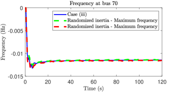
Figure 3: Frequency response at bus $70$ when: (i) case (iii) is implemented, with virtual inertia satisfying (14), (ii) the randomized scheme described by (14a), (15) is implemented, where green and red lines correspond to the maximum and minimum frequencies obtained after $500$ trials respectively.

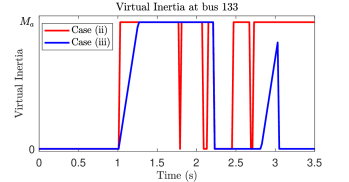
Figure 4: Virtual inertia at bus $133$ for cases (ii) and (iii) concerning inertia described by (13) and (14) and leading to oscillatory and stable responses respectively. After $3.5$ seconds, the virtual inertia is $M_{a}$ at almost all times, i.e. with fast fluctuations, for case (ii) and zero at all times for case (iii).

To demonstrate that Assumption 4 enables fast changes in inertia, the virtual inertia at bus $133$ concerning cases (ii) and (iii) is depicted in Fig. 4. From Fig. 4, it follows that for case (iii), the maximum virtual inertia support is provided within $0.3$ seconds from the time the frequency overpasses $0.02$ Hz and is removed completely after $3.5$ seconds. By contrast, in case (ii) the virtual inertia instantly reaches $M_{a}$ at $1$ second but fluctuates between $0$ and $M_{a}$. Its fast fluctuations create frequency oscillations which lead to more inertia fluctuations due to (13), yielding the oscillatory frequency response depicted in Fig. 2.

To further demonstrate that the proposed conditions yield a stable response, we considered randomly changing inertia input set points described by:

$$u_{j}(t^{+})=\begin{cases}u_{j}(t),\text{ if}~{}\mathrm{mod}(t,0.5)\neq 0,\\ u_{j}(t)+0.5M_{a},\text{ if}~{}\mathrm{mod}(t,0.5)=0,r_{j}(t)\geq 0.5,\\ \max(u_{j}(t)-0.5M_{a},0),\text{ otherwise,}\end{cases}$$ (15)

where $t^{+}=\lim_{\epsilon\rightarrow 0}(t+\epsilon)$ and $r_{j}(t)$ is randomly selected from the uniform distribution $[0,1]$ at each $t$ that satisfies $\mathrm{mod}(t,0.5)=0$. The scheme in (15) updates the set points $u_{j}$ every $0.5$ seconds by equiprobably increasing or decreasing their values by $0.5M_{a}$. Simultaneously, it ensures that the set points take non-negative values. The dynamics (14a), (15) were implemented and simulated $500$ times on the same setting as cases (ii) and (iii), to show that stability is preserved for a wide range of varying virtual inertia profiles that satisfy Assumption 4. The latter is demonstrated in Fig. 3, which shows that the maximum and minimum frequencies obtained with the presented randomized scheme are very close to the response associated with case (iii).

VII-A3 Instability inducing single-bus varying inertia

To demonstrate that local inertia variations may result in unstable behaviour, we performed simulations on the above described setting and considered a very small disturbance of magnitude $0.05$ p.u. (base 100MVA) at load buses $2$ and $3$ at $t=1$ second. In addition, we considered no virtual inertia at all buses except bus $23$. The design of the virtual inertia trajectory at bus $23$ followed the arguments in the proof of Theorem 2. In particular, the virtual inertia shifted between a set of large values and zero when the frequency deviations from the nominal value were large and small respectively. The virtual inertia trajectory at bus $23$ is depicted in Fig. 5. As follows from Fig. 5, the virtual inertia is piecewise-constant and takes zero values for short durations of time. The frequency response for the considered case is presented in Fig. 6, which depicts increasing frequency oscillations as time grows which eventually lead to instability after approximately 35 seconds. The presence of increasing frequency deviations from equilibrium is in agreement with Assumption 5(ii), which is a main condition to deduce instability. These results verify the analysis presented in Section VI.

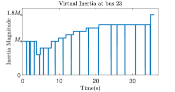
Figure 5: Virtual inertia at bus $23$ that resulted in unstable behaviour under constant inertia in the remaining power network.

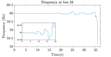
Figure 6: Frequency response at bus $23$ when varying virtual inertia is present at bus $23$ and no virtual inertia is present in the remaining buses.

VII-B Simulations on the IEEE New York / New England 68-bus system

The IEEE New York / New England system contains $52$ load buses serving different types of loads including constant active and reactive loads and $16$ generation buses. The overall system has a total real power of $16.41$ GW. For our simulation, we considered a step increase in demand of magnitude $2$ p.u. at load buses $2$ and $3$ at $t=1$ second. The time precision of the simulation was $0.01$ seconds.

In analogy to Section VII-A, we aimed to demonstrate how varying inertia may induce large frequency oscillations and that the application of the proposed conditions enables a stable response. We considered the following three cases:

1. The presence of no virtual inertia.

2. The presence of virtual inertia in all generation buses, with dynamics described by (13), where $M_{a}=20$ seconds.

3. The presence of virtual inertia in all generation buses with dynamics described by (14), where $M_{a}=20$ seconds and $\tau=100\text{s}^{-1}$.

Case (ii) includes fast varying, frequency dependent inertia trajectories, which do not abide by the conditions presented in this paper. On the other hand, case (iii) includes inertia with variations bounded by the local strictness constant $\rho_{j}$.

The frequency response at bus $23$ for the three considered cases is depicted in Fig. 7. From Fig. 7, it follows that case (ii) yields an oscillatory frequency response, demonstrating how fast inertia oscillations may cause stability issues. On the other hand, a stable response was observed when case (iii) was implemented. The latter demonstrates how imposing a suitable bound on the rate of change of inertia may enable a stable response and verifies the analysis presented in Section IV.

To demonstrate how local inertia variations may result in unstable behaviour, we simulated the above described setting with a very small load disturbance of magnitude $0.01$ p.u. at load buses $2$ and $3$ at $t=1$ second. In addition, we considered varying inertia at bus $57$ and constant inertia at all remaining buses. Similar to Section VII-A, the design of the virtual inertia trajectory at bus $57$ followed the arguments in the proof of Theorem 2, i.e. large inertia values were employed during large frequency deviations and no virtual inertia was considered otherwise. The frequency response at a randomly selected bus (bus $20$) is presented in Fig. 8. Figure 8 depicts growing oscillations, caused due to the inertia variations at bus $57$. Considering that such response follows from a normally negligible disturbance (of $2$ MW) demonstrates the capability of local inertia variations to cause instability in power networks and verifies the analysis presented in Section VI.

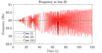
Figure 7: Frequency response at bus $23$ when: (i) no virtual inertia is present, (ii) virtual inertia with dynamics described by (13) is included in all generation buses and (iii) virtual inertia with dynamics described by (14) is included in all generation buses.

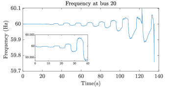
Figure 8: Frequency response at bus $20$ when varying virtual inertia is present at bus $57$ and no virtual inertia is present at the remaining buses.

VIII Conclusion

We have investigated the stability properties of power networks with time-varying inertia within the primary frequency control timeframe. In particular, we considered the interaction between the frequency dynamics and a wide class of non-linear power supply dynamics at the presence of time-varying inertia. For the considered system, we provided asymptotic stability guarantees under two proposed conditions. The first condition required that the aggregate power supply dynamics at each bus satisfied a passivity related property. The second condition set a constraint on the maximum rate of growth of inertia that was associated with the local power supply dynamics. The proposed conditions are decentralized and applicable to arbitrary network topologies and may be used for the design of practical guidelines for virtual inertia schemes that will improve the reliability and enhance the stability properties of the power grid. In addition, to demonstrate their applicability, we explain how these conditions can be efficiently verified for linear power supply dynamics by solving a suitable linear matrix inequality optimization problem. Our stability analysis is complemented with further analytic results that demonstrate how single-bus inertia variations may lead to instability. Numerical simulations on the NPCC 140-bus and New York/ New England 68-bus systems offered additional motivation and validated our analytic results. In particular, the simulation results demonstrated how varying virtual inertia may induce large frequency oscillations and verified that the application of the proposed conditions resulted in a stable response. In addition, they illustrate how single-bus inertia variations may lead to unstable power system behaviour.

Appendix

This appendix includes the proofs of Lemmas 1 and 2, Theorems 1 and 2 and Corollary 1. Additionally, it includes Propositions 1, 2 and 3 that facilitate the proof of Theorem 2.

Proof of Lemma 1: Existence of a unique solution $\beta(t)$ to (4)–(5) for all $t\geq 0$ requires [29, Ch. 4.3] that (i) (4)–(5) is continuous in $t$ and $\beta$, and (ii) (4)–(5) is locally Lipschitz in $\beta$ uniformly in $t\in[0,\infty)$. Condition (i) is satisfied from Assumption 3 and the continuity of (4)–(5) in $\beta$. Condition (ii) is satisfied since (4)–(5) is locally Lipschitz in $\beta$ for given $t$ and the fact that $M_{j}(t)\geq M^{0}_{j}>0$ for all times which allows a uniform local Lipschitz constant to be obtained for all $t\geq 0$. Hence, for any initial condition $\beta(0)\in\mathbb{R}^{m}$ there exists a unique solution $\beta(t),t\geq 0$ to (4)–(5). $\blacksquare$

Proof of Theorem 1: We will use Lyapunov arguments to prove Theorem 1 by treating (4)–(5) as a time-varying system with time-dependent parameter $M(t)$.

First, we consider the function

$$V_{F}(M,\omega)=\frac{1}{2}\sum_{j\in\mathcal{N}}M_{j}(t)(\omega_{j}-\omega^{*}_{j})^{2},$$

with time derivative along trajectories of (1b) given by

$$\dot{V}_{F} =\sum_{j\in\mathcal{N}}[\frac{\dot{M}_{j}}{2}(\omega_{j}-\omega^{*}_{j})^{2}$$

$$+(\omega_{j}-\omega^{*}_{j})(-p_{j}^{L}+s_{j}-\sum_{k\in\mathcal{N}^{s}_{j}}p_{jk}+\sum_{l\in\mathcal{N}^{p}_{j}}p_{lj})],$$ (16)

In addition, we consider the function

$${P}(\eta)=\sum_{(k,l)\in\mathcal{E}}\int_{\eta^{*}_{kl}}^{\eta_{kl}}B_{kl}(\sin\phi-\sin\eta^{*}_{kl})d\phi.$$

From (1a) and (1c), the derivative of $V_{P}$ is given by

$$\dot{V}_{P} =\sum_{(k,l)\in\mathcal{E}}B_{kl}(\sin\eta_{kl}-\sin\eta^{*}_{kl})(\omega_{k}-\omega_{l})$$

$$=\sum_{(k,l)\in\mathcal{E}}(p_{kl}-p^{*}_{kl})(\omega_{k}-\omega_{l}).$$ (17)

Furthermore, from Assumption 2 and Definition 2, it follows that there exist open neighbourhoods $\Omega_{j}$ of $\omega^{*}_{j}$ and $X_{j}$ of $x^{s,*}_{j}$ and continuously differentiable, positive semidefinite functions $V_{j}(x^{s}_{j})$ such that

$$\dot{V}_{j}\leq((-\omega_{j})-(-\omega^{*}_{j}))(s_{j}-s^{*}_{j})-\rho_{j}((-\omega_{j})-(-\omega^{*}_{j}))^{2},$$ (18)

where $\rho_{j}>0$, for all $\omega_{j}\in\Omega_{j},x^{s}_{j}\in X_{j}$ and for each $j\in\mathcal{N}$. We now consider the following Lyapunov candidate function

$$V(M,\beta)=V_{F}(M,\omega)+V_{P}(\eta)+\sum_{j\in\mathcal{N}}V_{j}(x^{s}_{j}),$$ (19)

reminding that $\beta=(\omega,\eta,x^{s})$. Using (16)–(18) it follows that when $\omega_{j}\in\Omega_{j},x^{s}_{j}\in X_{j},j\in\mathcal{N}$, then

$$\dot{V}\leq\sum_{j\in\mathcal{N}}(\dot{M}_{j}/2-\rho_{j})(\omega_{j}-\omega^{*}_{j})^{2}\leq 0,$$ (20)

where the first part follows by applying (6b) on (16) and the second from Assumption 4.

Function $V_{F}$ has a global minimum at $\omega=\omega^{*}$. In addition, Assumption 1 guarantees the existence of a neighbourhood of $\eta^{*}$ where $V_{P}$ is increasing, which suggests that $V_{P}$ has a strict local minimum at $\eta^{*}$. Moreover, from Assumption 2 and Definition 2 it follows that each $V_{j},j\in\mathcal{N}$ has a strict local minimum at $x^{s,*}_{j}$. Hence, $V$ has a local minimum at $\beta^{*}=(\omega^{*},\eta^{*},x^{s,*})$ that is independent of the value of $M(t)$, since $M_{j}(t)\geq M^{0}_{j}>0,t\geq 0,j\in\mathcal{N}$. In addition, $\beta^{*}$ is a strict minimum associated with the states, i.e. locally the set $\{\bar{\beta}:\bar{\beta}=\operatorname*{arg\,min}_{\beta}V(M,\beta),\forall M\in S:=\bigcup_{j\in\mathcal{N}}[M^{0}_{j},\infty)\}$ contains $\beta^{*}$ only.

We can now choose a neighbourhood of $\beta^{*}$, denoted by $B$, such that (i) $\omega_{j}\in\Omega_{j},j\in\mathcal{N}$, (ii) $x^{s}_{j}\in X_{j},j\in\mathcal{N}$, and (iii) all $x^{s}_{j},j\in\mathcal{N}$ lie in their respective neighbourhoods $\Psi_{j}$, as defined in Section II-B. Hence, it follows that for all $(M,\beta)\in S\times B$, $V$ is a non-increasing function with a strict local minimum associated with the states at $\beta^{*}$. Therefore, the set $\Xi=\{\beta:\exists M\in S\text{ such that }V\leq\epsilon,V\text{ connected}\}$ containing $\beta^{*}$ is both compact and positively invariant with respect to (4)–(5) when $\epsilon>0$ is sufficiently small.

We can now apply [29, Theorem 4.2] with the Lyapunov function $V$ and the invariant set $\Xi$ for the solutions $\beta(t),t\geq 0$ of (4)–(5). From this result, we deduce that for any $(M(0),\beta(0))\in S\times\Xi$ it follows that $\beta\rightarrow Q$ as $t\rightarrow\infty$, where $Q$ is the largest invariant set within $\Xi\cap\{\beta:\dot{V}=0\}$. Within this set, it holds that $\omega_{j}=\omega^{*}_{j},j\in\mathcal{N}$ from (20), which implies that (6a), (6b) and (6d) hold. It hence follows that $\eta$ converges to a constant value $\bar{\eta}$. In addition, the definitions in Section II-B suggest that $\omega=\omega^{*}$ implies the convergence of $x^{s}$ to $x^{s,*}$. Therefore, we conclude that all solutions $\beta(t),t\geq 0$ of (4)–(5) initiated in $\Xi$ converge to the set of equilibrium points within $\Xi$. The latter completes the proof. $\blacksquare$

Proof of Lemma 2: The proof follows directly from the proof of Theorem 1 by letting $V_{P}(\eta)=\sum_{(k,l)\in\mathcal{E}}B_{kl}(\eta_{kl}-\eta^{*}_{kl})^{2}/2$. In particular, it follows that locally around the considered equilibrium, solutions to (5), (11) satisfy (20). The rest of the arguments follow in analogy to the proof of Theorem 1. $\blacksquare$

To facilitate the analysis associated with the instability results presented in Section VI, we consider the effect of having some bus $k$ with a fixed frequency $\bar{\omega}$ within system (5), (11). The dynamics of such a system are described below:

$$\dot{\eta} =H^{T}\omega,$$ (21a)

$$M_{j}\dot{\omega}_{j} =-p^{L}_{j}+s_{j}-\sum_{k\in\mathcal{N}^{s}_{j}}p_{jk}+\sum_{l\in\mathcal{N}^{p}_{j}}p_{lj},j\in\mathcal{N}\setminus\{k\},$$ (21b)

$$\omega_{k} =\bar{\omega},$$ (21c)

$$p =B\eta.$$ (21d)

The system represented by (21) aims to describe the behaviour of (11), when the inertia of bus $k$ is infinite and $\omega_{k}(0)=\bar{\omega}$. Although the assumption of infinite inertia is unrealistic, the trajectories of (5), (21) approximate those of (5), (11) for a long time interval when the inertia at bus $k$ is sufficiently large. The latter enables to explore several properties of (5), (11) and facilitates our instability analysis.

It should be noted that there is a direct relation between (21) and the analysis presented in Section VI, since it can be trivially shown that $\gamma$-points, defined in Definition 4, coincide with the equilibria to (5), (21).

The following proposition demonstrates the convergence of solutions to (5), (21) to the set of its equilibria, similarly to Theorem 1. In addition, it provides conditions that allow to deduce convergence to an equilibrium point of (5), (21). It should be clarified that within Proposition 1, and also Proposition 2 below, Assumptions 3, 4 refer to all buses besides bus $k$. The latter follows since no inertia is defined for bus $k$.

Proposition 1

Let Assumptions 3 and 4 hold and consider an equilibrium of (5), (21) where Assumption 2 holds. Then, there exists an open neighbourhood $\Xi$ containing that equilibrium such that

1. solutions $\beta(t),t\geq 0$ to (5), (21) initiated in $\Xi$ asymptotically converge to the set of equilibria within $\Xi$,

2. if Assumption 2 holds for all equilibria within $\Xi$, then solutions $\beta(t),t\geq 0$ to (5), (21) initiated in $\Xi$ converge to an equilibrium point within $\Xi$.

Proof of Proposition 1: The proof is split in two parts, regarding each statement in Proposition 1.

Part (i): The proof follows by using Lyapunov arguments, similar to the proof of Theorem 1, by treating (5), (21) as a time-varying system.

First, we consider the function

$$V_{G}(M,\omega)=\frac{1}{2}\sum_{j\in\mathcal{N}\setminus\{k\}}M_{j}(t)(\omega_{j}-\omega^{*}_{j})^{2},$$

with time derivative along trajectories of (21b) given by

$$\dot{V}_{G} =\sum_{j\in\mathcal{N}\setminus\{k\}}[\frac{\dot{M}_{j}}{2}(\omega_{j}-\omega^{*}_{j})^{2}$$

$$+(\omega_{j}-\omega^{*}_{j})(-p_{j}^{L}+s_{j}-\sum_{k\in\mathcal{N}^{s}_{j}}p_{jk}+\sum_{l\in\mathcal{N}^{p}_{j}}p_{lj})].$$ (22)

In addition, we consider the function $V_{H}(\eta)=\sum_{(k,l)\in\mathcal{E}}B_{kl}(\eta_{kl}-\eta^{*}_{kl})^{2}/2$, with derivative given by (21a) and (21d) as

$$\dot{V}_{H} =\sum_{(m,l)\in\mathcal{E}}(p_{ml}-p^{*}_{kl})(\omega_{m}-\omega_{l}).$$ (23)

Furthermore, from Assumption 2 and Definition 2, it follows that there exist open neighbourhoods $\Omega_{j}$ of $\omega^{*}_{j}$ and $X_{j}$ of $x^{s,*}_{j}$ and continuously differentiable, positive semidefinite functions $V_{j}(x^{s}_{j})$ such that (18) holds.

We now consider the following Lyapunov candidate

$$V(M,\beta)=V_{G}(M,\omega)+V_{H}(\eta)+\sum_{j\in\mathcal{N}}V_{j}(x^{s}_{j}),$$

reminding that $\beta=(\omega,\eta,x^{s})$. Using (18), (22), (23) it follows that

$$\dot{V}\leq\sum_{j\in\mathcal{N}\setminus\{k\}}(\dot{M}_{j}/2-\rho_{j})(\omega_{j}-\omega^{*}_{j})^{2}\leq 0,$$ (24)

by applying (6b) on (22) and using Assumption 4.

We then define a compact set $\Xi$ that includes $\beta^{*}$ in analogy to the proof of Theorem 1. Using [29, Theorem 4.2] and similar arguments as in the proof of Theorem 1, it follows that solutions initiated in $\Xi$ converge to the set of equilibria within $\Xi$ as $t\rightarrow\infty$.

Part (ii): Part (i) proved that solutions initiated in $\Xi$ converge to the set of equilibria within $\Xi$ and that $\Xi$ is a compact invariant set of (5), (21). Hence, the considered equilibrium point is Lyapunov stable [29, Definition 3.1]. Now if Assumption 2 holds for all equilibria within $\Xi$ it follows that these equilibria are also Lyapunov stable. The latter allows to use [29, Th. 4.20] to deduce that all solutions starting in $\Xi$ converge to an equilibrium point within $\Xi$. $\blacksquare$

The following proposition, shows that system (5), (21) has arbitrarily long periods of time where all bus frequencies lie within a ball of size $\epsilon$ from $\bar{\omega}$, for any positive value of $\epsilon$.

Proposition 2

Let Assumptions 3 and 4 hold and consider an equilibrium of (5), (21) where Assumption 2 holds. Then, there exists an open neighbourhood $\Xi$ containing that equilibrium such that for any solution $\beta(t),t\geq 0$ to (5), (21) initiated in $\Xi$ and any $\tau,\epsilon\in\mathbb{R}_{+}$ there exists some $\hat{\tau}\in\mathbb{R}_{+}$ such that $\omega_{j}(t)\in\mathcal{B}(\bar{\omega},\epsilon),t\in[\hat{\tau},\hat{\tau}+\tau],j\in\mathcal{N}$.

Proof of Proposition 2: First note that the results presented in Proposition 1 hold, since all associated assumptions are satisfied. Then, from (24) and the Lipschitz continuity of (5), (21), it follows that for any $\tau,\epsilon\in\mathbb{R}_{+}$ there exists some $\delta>0$ such that for any $\bar{\tau}$, if $\omega_{j}(t)\notin\mathcal{B}(\bar{\omega},\epsilon)$ for some $j\in\mathcal{N}$ and some $t\in[\bar{\tau},\bar{\tau}+\tau]$ then $V(\bar{\tau}+\tau)\leq V(\bar{\tau})-\delta$. Noting that $V(0)$ is bounded and $V(t)\geq 0,t\geq 0$ allows to deduce the above result by contradiction. $\blacksquare$

The following proposition states the existence of a virtual inertia trajectory $M^{v}_{k}(t),t\geq 0$ such that solutions to (5), (11) and (5), (21) are arbitrarily close for arbitrarily long, but finite, time intervals. For convenience in presentation, we consider $\omega_{k}$ as a state of system (5), (21) that keeps a constant value at all times. The latter suggests that the statement regarding the initial conditions of (5), (11) and (5), (21) implies that $\omega_{k}(0)=\bar{\omega}$. In addition, by slightly abusing notation, we denote trajectories of (5), (11) and (5), (21) by $\beta(t)$ and $\hat{\beta}(t)$ respectively.

Proposition 3

Let Assumption 3 hold. Then, for any $\tau,\epsilon\in~{}\mathbb{R}_{+}$ and any bounded trajectory for $M^{v}_{j}(t),j\in\mathcal{N}\setminus\{k\},t\geq 0$, there exists a trajectory for $M^{v}_{k}(t),t\geq 0$ such that solutions to (5), (11) and (5), (21) with $\beta(0)=\hat{\beta}(0)$ satisfy $\left\lVert\beta(t)-\hat{\beta}(t)\right\rVert\leq\epsilon,t\in[0,\tau]$.

Proof of Proposition 3: First note that both (5), (11) and (5), (21) are locally Lipschitz due to Assumption 3 and the conditions on (5). The proof follows by considering (11) and noting that when $M^{v}_{k}\rightarrow\infty$ the frequency derivative at bus $k$ tends to zero and hence the frequency at bus $k$ is constant. Hence, for any bounded trajectory for $M^{v}_{j}(t),j\in\mathcal{N}\setminus\{k\},t\geq 0$, when $\omega_{k}(0)=\bar{\omega}$ and $M^{v}_{k}=\infty$ the dynamics described by (11) and (21) are identical. The latter suggests the existence of sufficiently large, but finite, value $\bar{M}$ such that for any finite time $\tau$ and any $\epsilon>0$, $M^{v}_{k}(t)\geq\bar{M},t\in[0,\tau]$ implies that $\left\lVert\beta(t)-\hat{\beta}(t)\right\rVert\leq\epsilon,t\leq\tau$. The latter completes the proof. $\blacksquare$

Proof of Theorem 2: To prove Theorem 2, we will define an iterative process and provide properties for the trajectory of $M_{k}$ such that there exist sequences of time instants $\hat{t}_{i},i\in\mathbb{N}_{+}$ and positive values $\phi_{i},i\in\mathbb{N}_{+}$ satisfying $\hat{t}_{i}>\hat{t}_{j},i>j$ and $\phi_{i}>\phi_{j},i>j$ such that $\beta(\hat{t}_{i})\notin\mathcal{B}(\gamma,\phi_{i}),\gamma\in\Gamma(\omega^{s,\ast}),i\in\mathbb{N}_{+}$. In addition, we will demonstrate the existence of some finite iteration $n$ such that $\phi_{n}\geq\Phi$, where $\Phi>0$ is defined in Assumption 5.

From the theorem statement, it is assumed that $|\omega_{k}(0)-\omega^{s,\ast}|=\delta$. Then consider Proposition 3. The latter claims that for any finite $\epsilon_{1},\tau$, there exists a trajectory for $M^{v}_{k}(t)$ such that solutions to (5), (11) and (5), (21) with the same initial conditions have a distance of at most $\epsilon_{1}$, for $t\leq\tau$. In addition, from Proposition 2 it follows that for any $\tau_{2},\epsilon_{2}\in\mathbb{R}_{+}$ there exists some $\hat{\tau}_{2}\in\mathbb{R}_{+}$ such that $\omega_{j}(t)\in\mathcal{B}(\bar{\omega},\epsilon),t\in[\hat{\tau}_{2},\hat{\tau}_{2}+\tau_{2}],j\in\mathcal{N}$. Using the previous argument and letting $\bar{\omega}=\omega_{k}(0)$ suggests that solutions to (5), (11) satisfy $\omega_{j}(t)\in\mathcal{B}(\bar{\omega},\epsilon),t\in[\hat{\tau}_{2},\hat{\tau}_{2}+\tau_{2}],j\in\mathcal{N}$, where $\epsilon=\epsilon_{1}+\epsilon_{2}$. Assumption 5(i) suggests the existence of some finite $\hat{\tau}$ such that the previous statement implies that $\beta(\hat{\tau})\in\mathcal{B}(\gamma,\hat{\epsilon}),\gamma\in\Gamma(\bar{\omega}),\hat{\epsilon}>0$. The latter additionally requires that $\tau\geq\hat{\tau}$ which can be achieved by suitably selecting $M^{v}_{k}$ following Proposition 3.

We now define $\hat{t}_{1}=\tau$ and $\bar{\omega}^{1}=\delta$. From Assumption 5(ii), there exists some $\tau^{1}$ such that $M_{k}(t)=M^{0}_{k},t\in[\hat{t}_{1},\hat{t}_{1}+\tau^{1}]$ implies that solutions to (5), (11) satisfy $|\omega_{k}(\hat{t}_{1}+\tau^{1})-\omega^{s,\ast}|>\bar{\omega}^{1}+\bar{\epsilon},\bar{\epsilon}>\hat{\epsilon}$. If for some $t\in[\hat{t}_{1},\hat{t}_{1}+\tau^{1}]$ it holds that $\beta(\tilde{t})\notin\mathcal{B}(\gamma,\Phi),\gamma\in\Gamma(\omega^{s,\ast})$ then the proof is complete. Otherwise, we let $\phi_{1}=\bar{\omega}^{1}+\bar{\epsilon}$, set a sufficiently large value for $M^{v}_{k}$ at $t=\hat{t}_{1}+\tau^{1}$, as follows from Proposition 3, and repeat the above process iteratively, using Assumption 5(iii) to deduce the convergence arguments associated with Proposition 1. This process creates a sequence of time instants $\hat{t}_{l}$, associated with each iteration $l\in\mathbb{N}_{+}$, satisfying $\hat{t}_{l+1}>\hat{t}_{l}$, such that $|\omega_{k}(t_{l+1})-\omega^{s,\ast}|\geq|\omega_{k}(t_{l})-\omega^{s,\ast}|+\bar{\epsilon}-\hat{\epsilon}$, which implies that $\phi_{l+1}>\phi_{l}+\bar{\epsilon}-\hat{\epsilon}$.

Since the value of $\Phi$ is bounded, this will be reached in a finite amount of iterations (no more than $\Phi/(\bar{\epsilon}-\hat{\epsilon})$). Since the time required for each iteration is finite, then there exists some finite time $\bar{t}$ such that $\beta(\bar{t})\notin\mathcal{B}(\gamma,\Phi),\gamma\in\Gamma(\omega^{s,\ast})$. Noting that no assumption is made for the magnitude of $\delta$, and hence that the above arguments hold for any $\delta>0$, completes the proof. $\blacksquare$

Proof of Corollary 1: The proof follows directly from Theorem 2 which makes the same assumptions. In particular, an unstable equilibrium is defined as an equilibrium that is not stable, e.g. [29, Dfn. 4.1]. For a system described by $\dot{x}=f(x)$, a stable equilibrium satisfies the property that for any $\epsilon>0$, there exists some $\delta>0$ such that $\left\lVert x(0)\right\rVert<\delta$ implies $\left\lVert x(t)\right\rVert<\epsilon,t\geq 0$. Theorem 2 states that for any $\delta>0$, there exists an inertia trajectory at bus $k$ such that $|\omega_{k}-\omega^{s,\ast}|\geq\Phi$. The latter suggests that under specific inertia trajectories, there exists some $\epsilon$ (i.e. any $\epsilon<\Phi$) such that there does not exist any $\delta>0$ such that the resulting trajectories for (5), (11) are bounded by $\epsilon$. The latter completes the proof. $\blacksquare$

References

- [1] A. Kasis, S. Timotheou, and M. Polycarpou, “Stability of power networks with time-varying inertia,” in 60th IEEE Conference on Decision and Control (CDC), 2021.
- [2] H. Lund, “Large-scale integration of optimal combinations of pv, wind and wave power into the electricity supply,” Renewable Energy, vol. 31, no. 4, pp. 503–515, 2006.
- [3] A. Ipakchi and F. Albuyeh, “Grid of the future,” IEEE Power and Energy magazine, vol. 7, no. 2, pp. 52–62, 2009.
- [4] P. Tielens and D. Van Hertem, “The relevance of inertia in power systems,” Renewable and Sustainable Energy Reviews, vol. 55, pp. 999–1009, 2016.
- [5] G. Lalor, J. Ritchie, S. Rourke, D. Flynn, and M. J. O’Malley, “Dynamic frequency control with increasing wind generation,” in IEEE Power Engineering Society General Meeting, 2004., pp. 1715–1720, IEEE, 2004.
- [6] A. Ulbig, T. S. Borsche, and G. Andersson, “Impact of low rotational inertia on power system stability and operation,” IFAC Proceedings Volumes, vol. 47, no. 3, pp. 7290–7297, 2014.
- [7] R.-C. S. P. . D. S. Group, “Frequency stability evaluation criteria for the synchronous zone of continental europe,” ENTSO-E, 2016.
- [8] J. Fang, H. Li, Y. Tang, and F. Blaabjerg, “Distributed power system virtual inertia implemented by grid-connected power converters,” IEEE Transactions on Power Electronics, vol. 33, no. 10, pp. 8488–8499, 2017.
- [9] Q.-C. Zhong and G. Weiss, “Synchronverters: Inverters that mimic synchronous generators,” IEEE Transactions on Industrial Electronics, vol. 58, no. 4, pp. 1259–1267, 2010.
- [10] C. Arghir, T. Jouini, and F. Dörfler, “Grid-forming control for power converters based on matching of synchronous machines,” Automatica, vol. 95, pp. 273–282, 2018.
- [11] T. V. Van, K. Visscher, J. Diaz, V. Karapanos, A. Woyte, M. Albu, J. Bozelie, T. Loix, and D. Federenciuc, “Virtual synchronous generator: An element of future grids,” in 2010 IEEE PES Innovative Smart Grid Technologies Conference Europe (ISGT Europe), pp. 1–7, IEEE, 2010.
- [12] M. Torres and L. A. Lopes, “Virtual synchronous generator control in autonomous wind-diesel power systems,” in 2009 IEEE Electrical Power & Energy Conference (EPEC), pp. 1–6, IEEE, 2009.
- [13] J. Alipoor, Y. Miura, and T. Ise, “Power system stabilization using virtual synchronous generator with alternating moment of inertia,” IEEE journal of Emerging and Selected Topics in Power Electronics, vol. 3, no. 2, pp. 451–458, 2014.
- [14] D. Chen, Y. Xu, and A. Q. Huang, “Integration of dc microgrids as virtual synchronous machines into the ac grid,” IEEE Transactions on Industrial Electronics, vol. 64, no. 9, pp. 7455–7466, 2017.
- [15] L. A. Lopes et al., “Self-tuning virtual synchronous machine: A control strategy for energy storage systems to support dynamic frequency control,” IEEE Transactions on Energy Conversion, vol. 29, no. 4, pp. 833–840, 2014.
- [16] J. Morren, S. W. De Haan, W. L. Kling, and J. Ferreira, “Wind turbines emulating inertia and supporting primary frequency control,” IEEE Transactions on Power Systems, vol. 21, no. 1, pp. 433–434, 2006.
- [17] F. M. Hughes, O. Anaya-Lara, N. Jenkins, and G. Strbac, “Control of dfig-based wind generation for power network support,” IEEE Transactions on Power Systems, vol. 20, no. 4, pp. 1958–1966, 2005.
- [18] J. Ekanayake and N. Jenkins, “Comparison of the response of doubly fed and fixed-speed induction generator wind turbines to changes in network frequency,” IEEE Transactions on Energy conversion, vol. 19, no. 4, pp. 800–802, 2004.
- [19] B. K. Poolla, S. Bolognani, and F. Dörfler, “Optimal placement of virtual inertia in power grids,” IEEE Transactions on Automatic Control, vol. 62, no. 12, pp. 6209–6220, 2017.
- [20] U. Tamrakar, D. Shrestha, M. Maharjan, B. P. Bhattarai, T. M. Hansen, and R. Tonkoski, “Virtual inertia: Current trends and future directions,” Applied Sciences, vol. 7, no. 7, p. 654, 2017.
- [21] S. D’Arco and J. A. Suul, “Virtual synchronous machines—classification of implementations and analysis of equivalence to droop controllers for microgrids,” in 2013 IEEE Grenoble Conference, pp. 1–7, IEEE, 2013.
- [22] G. S. Misyris, S. Chatzivasileiadis, and T. Weckesser, “Robust frequency control for varying inertia power systems,” in 2018 IEEE PES Innovative Smart Grid Technologies Conference Europe (ISGT-Europe), pp. 1–6, IEEE, 2018.
- [23] P. Hidalgo-Gonzalez, D. S. Callaway, R. Dobbe, R. Henriquez-Auba, and C. J. Tomlin, “Frequency regulation in hybrid power dynamics with variable and low inertia due to renewable energy,” in 2018 IEEE Conference on Decision and Control (CDC), pp. 1592–1597, IEEE, 2018.
- [24] T. S. Borsche, T. Liu, and D. J. Hill, “Effects of rotational inertia on power system damping and frequency transients,” in 2015 54th IEEE conference on decision and control (CDC), pp. 5940–5946, IEEE, 2015.
- [25] P. Srivastava, P. Hidalgo-Gonzalez, and J. Cortés, “Learning constant-gain stabilizing controllers for frequency regulation under variable inertia,” IEEE Control Systems Letters, 2022.
- [26] Y.-K. Wu, W.-H. Yang, Y.-L. Hu, and P. Q. Dzung, “Frequency regulation at a wind farm using time-varying inertia and droop controls,” IEEE Transactions on Industry Applications, vol. 55, no. 1, pp. 213–224, 2018.
- [27] J. Alipoor, Y. Miura, and T. Ise, “Distributed generation grid integration using virtual synchronous generator with adoptive virtual inertia,” in 2013 IEEE Energy Conversion Congress and Exposition, pp. 4546–4552, IEEE, 2013.
- [28] A. Kasis, E. Devane, C. Spanias, and I. Lestas, “Primary frequency regulation with load-side participation—part i: Stability and optimality,” IEEE Transactions on Power Systems, vol. 32, no. 5, pp. 3505–3518, 2016.
- [29] W. M. Haddad and V. Chellaboina, Nonlinear dynamical systems and control: a Lyapunov-based approach. Princeton university press, 2011.
- [30] A. Kasis, N. Monshizadeh, E. Devane, and I. Lestas, “Stability and optimality of distributed secondary frequency control schemes in power networks,” IEEE Transactions on Smart Grid, vol. 10, no. 2, pp. 1747–1761, 2017.
- [31] C. Zhao, U. Topcu, N. Li, and S. Low, “Design and stability of load-side primary frequency control in power systems,” IEEE Transactions on Automatic Control, vol. 59, no. 5, pp. 1177–1189, 2014.
- [32] J. Machowski, J. Bialek, and J. Bumby, Power system dynamics: stability and control. John Wiley & Sons, 2011.
- [33] F. Dörfler, M. Chertkov, and F. Bullo, “Synchronization in complex oscillator networks and smart grids,” Proceedings of the National Academy of Sciences, vol. 110, no. 6, pp. 2005–2010, 2013.
- [34] H. K. Khalil, Nonlinear systems, vol. 3. Prentice Hall New Jersey, 1996.
- [35] A. Kasis, N. Monshizadeh, and I. Lestas, “Secondary frequency control with on–off load side participation in power networks,” IEEE Transactions on Control of Network Systems, vol. 7, no. 2, pp. 603–613, 2019.
- [36] J. T. Wen and M. Arcak, “A unifying passivity framework for network flow control,” IEEE Transactions on Automatic Control, vol. 49, no. 2, pp. 162–174, 2004.
- [37] J. C. Willems, “Dissipative dynamical systems part ii: Linear systems with quadratic supply rates,” Archive for Rational Mechanics and Analysis, vol. 45, no. 5, pp. 352–393, 1972.
- [38] S. Trip and C. De Persis, “Distributed optimal load frequency control with non-passive dynamics,” IEEE Transactions on Control of Network Systems, vol. 5, no. 3, pp. 1232–1244, 2017.
- [39] K. Cheung, J. Chow, and G. Rogers, “Power system toolbox, v 3.0,” Rensselaer Polytechnic Institute and Cherry Tree Scientific Software, 2009.
- [40] M. Grant, S. Boyd, and Y. Ye, “Cvx users’ guide,” online: http://www. stanford. edu/~ boyd/software. html, 2009.