Schmidt decomposition of parity adapted coherent states for symmetric multi-quDits

Abstract

In this paper we study the entanglement in symmetric $N$-quDit systems. In particular we use generalizations to $U(D)$ of spin $U(2)$ coherent states and their projections on definite parity $\mathbbm{c}\in\mathbb{Z}_{2}^{D-1}$ (multicomponent Schrödinger cat) states and we analyse their reduced density matrices when tracing out $M<N$ quDits. The eigenvalues (or Schmidt coefficients) of these reduced density matrices are completely characterized, allowing to proof a theorem for the decomposition of a $N$-quDit Schrödinger cat state with a given parity $\mathbbm{c}$ into a sum over all possible parities of tensor products of Schrödinger cat states of $N-M$ and $M$ particles. Diverse asymptotic properties of the Schmidt eigenvalues are studied and, in particular, for the (rescaled) double thermodynamic limit ($N,M\rightarrow\infty,\,M/N$ fixed), we reproduce and generalize to quDits known results for photon loss of parity adapted coherent states of the harmonic oscillator, thus providing an unified Schmidt decomposition for both multi-quDits and (multi-mode) photons. These results allow to determine the entanglement properties of these states and also their decoherence properties under quDit loss, where we demonstrate the robustness of these states.

I Introduction

Coherent states (CS), either of the harmonic oscillator (HO) or for a spin system, have many applications in Quantum Mechanics and Quantum Optics (among many other fields), and in particular parity adapted CS (a particular instance of a Schrödinger cat state) for the HO or for $U(2)$ are interesting since they are used in many protocols in Quantum Information Processing or appear as the lower energy states in some nuclear or molecular models like the Dicke Dicke (1954) or Lipkin-Meshkov-Glick (LMG) models Lipkin et al. (1965).

We shall consider in this paper “spin” CS for $U(D)$ in its symmetric representation (i.e. made of a fixed number $N$ of indistinguishable quDits) and we shall construct from them parity adapted CS, i.e states which are invariant under the parity group. The parity group in the case of $U(D)$ is $\mathbb{Z}_{2}^{D-1}$, generalizing the case of $SU(2)$, where the parity group is simply $\mathbb{Z}_{2}=\{-1,+1\}$.

For applications, it is important to characterize the entanglement properties of these states, therefore we shall consider entropic entanglement measures in terms of the entropy of $M$-particle reduced density matrices (RDM), i.e. in terms of a bipartition of the $N$ quDits in $N-M$ and $M$ quDits and tracing out the $N-M$ subsystem.

There is an intense debate in the literature concerning the notion of entanglement in systems of identical and indistinguishable particles (like the case of symmetric multi-quDits). Some authors Benatti et al. (2020, 2021) consider that particle entanglement, obtained through RDM by tracing out a number of particles Wang and Mølmer (2002); Lo Franco and Compagno (2016); Sciara et al. (2017), cannot be used as a quantum resource in quantum information tasks for indistinguishable particles. Other authors consider that the entanglement due to exchange symmetry can indeed be useful in those tasks, providing some examples of it Killoran et al. (2014); Morris et al. (2020). The authors of Benatti et al. (2020, 2021) propose mode entanglement as the only meaningful way of defining entanglement for indistinguishable particles.

In this paper we shall consider the notion of particle entanglement in symmetric multi-quDit systems since it is mathematically consistent and physically justified in the case of parity adapted coherent states. The case of mode entanglement will be considered in a future work.

To characterize the entanglement of parity adapted $U(D)$ CS, we need to compute the Schmidt decomposition of these states when a bipartition in $N-M$ and $M$ particles is considered. The main result of this paper is that, under this decomposition, parity adapted CS decompose as the convolution over all possible parities, of tensor products of parity adapted CS of $N-M$ and $M$ particles. The coefficients of this decomposition (Schmidt coefficients) and their squares (Schmidt eigenvalues) are determined for all $N$ and $M$, and the main features of them and their behaviour under various limits are estudied. For a detailed account of these features, a variety of graphical tools are used, like contour plots, angular plots, etc., but, in the case of a large $D$, information diagrams (see Guerrero et al. (2022) and references therein) prove to be a valuable tool when appropriate colormaps are used (see the Supplementary Material).

The content of the paper is the following. In Sec. II the symmetric representation of $U(D)$ is reviewed in order to fix notation (second quantization approach), and parity transformations and parity projectors are introduced. In Sec. III CS for the symmetric representation of $U(D)$ are reviewed, and some results for their relation with identical tensor product states are given. In Sec. IV parity adapted CS are defined and some of their properties are given, in particular their behaviour under certain limits. In Sec. V we specify the entanglement measure used in this paper to study the entanglement properties of parity adapted CS. In Sec. VI the main result of this paper is proved, namely the Schmidt decomposition of parity adapted CS of $N$ particles into $N-M$ and $M$ particle subsystems, with the determination of the Schmidt coefficients and eigenvalues. In Sec. VII some limits for the Schmidt eigenvalues are studied. In Sec. VIII some physical appliations and possible methods to generate these states are given, in particular the interesting subject of quDit loss, where the Schmidt decomposition here provided can be of crucial importance. The paper ends with a conclusing section X. In the Supplementary Material, a reminder of the subject of information diagrams is included, and a exhaustive set of figures shown the entanglement properties of parity adapted CS for $D>2$ is provided.

II Symmetric representation of $\mathbf{U(D)}$

The fully symmetric representation of dimension $\tbinom{N+D-1}{N}$ of $U(D)$ can be realized as a system of $N$ identical and indistinguishable particles (atoms) with $D$ levels (internal states), that will be referred to as quDits, with levels labelled by $|0\rangle,\,|1\rangle,\,\ldots,|D-1\rangle$ (for $D=2$ we have the standard qubit usually labelled by $|0\rangle$,$|1\rangle$ or $|\uparrow\rangle$,$|\downarrow\rangle$).

Introducing the boson operators $a_{i},a_{i}^{\dagger}$ ($a_{i}^{\dagger}$ creates a quDit in the $i$-th level and $a_{i}$ annihilates it), the Lie algebra of $U(D)$ can be realized (in the Schwinger representation Schwinger (1952)) as:

$$S_{ij}=a^{\dagger}_{i}a_{j},\;i,j=0,\dots,D-1\,.$$ (1)

The operator $S_{ii}$ is the number operator for the population of the $i$-th level, and $S_{ij}$ ($i\neq j$) creates a quDit in the level $i$ and annihilates another one in the level $j$. Therefore $S_{ij}$ preserves the total number $N$ of quDits.

It is important to note that the $U(D)$ operators $S_{ij}$ are collective operators, in the sense that they do not act on the individual states of the particles (which can be an ill-defined concept due to symmetrization). They have in fact been built up using the second quantization formalism Dirac (1927); Fock (1932). They fulfill the commutation relations:

$$\left[S_{{ij}},S_{{kl}}\right]=\delta_{{jk}}S_{{il}}-\delta_{{il}}S_{{kj}}.$$ (2)

The carrier Hilbert space ${\cal H}_{N}$ of our symmetric $N$-quDit system is spanned by the Bose-Einstein-Fock basis states ($|\vec{0}\rangle$ denotes the Fock vacuum):

$$|\vec{n}\rangle=|n_{0},\dots,n_{D-1}\rangle=\frac{(a_{0}^{\dagger})^{n_{0}}\dots(a_{D-1}^{\dagger})^{n_{D-1}}}{\sqrt{n_{0}!\dots n_{D-1}!}}|\vec{0}\rangle\,,\qquad n_{0}+\dots+n_{D-1}=N\,,$$ (3)

where $n_{i}\geq 0$ denotes the occupancy number of the $i$th-level (the eigenvalue of $S_{ii}$), with the restriction given by the linear Casimir of $U(D)$, $C_{1}=\sum_{i=0}^{D-1}S_{ii}$, the total number of quDits. The expansion of a general symmetric $N$-quDit state $\psi$ in the Fock basis will be written as

$$|\psi\rangle=\sum_{\|\vec{n}\|_{1}=N}\,c_{\vec{n}}|\vec{n}\rangle,$$ (4)

where the sum is restricted to those $\vec{n}$ such that $\|\vec{n}\|_{1}=n_{0}+\dots+n_{D-1}=N$.

In order to define the notion of entanglement, we shall consider in ${\cal H}_{N}$ various families of states. The simplest states that one usually introduces, in order to define separable (non-entangled) states, are Tensor Product States (TPS) $|\vec{\psi}\rangle^{(N)}=|\psi_{1}\rangle\otimes\cdots\otimes|\psi_{N}\rangle$. However, due to the exchange symmetry, in ${\cal H}_{N}$ the only TPS are the subset of identical tensor product states (ITPS):

$${\cal A}_{N}^{ITPS}=\{|\psi\;\rangle^{\otimes N}\in{\cal H}_{N}\,:\,|\psi\rangle^{\otimes N}=|\psi\rangle\otimes\stackrel{{\scriptstyle N}}{{\cdots}}\otimes|\psi\rangle\}\subset{\cal H}_{N}\,.$$ (5)

with $|\psi\rangle\in{\cal H}_{1}$. If the one-quDit state $|\psi\rangle\in{\cal H}_{1}$ is expressed as:

$$|\psi\rangle=w_{0}|0\rangle+w_{1}|1\rangle+\cdots+w_{D-1}|D-1\rangle\equiv|w_{0},w_{1},\ldots,w_{D-1}\rangle\equiv|\bm{w}\rangle\,,\qquad|w_{0}|^{2}+|w_{1}|^{2}\cdots+|w_{D-1}|^{2}=1\,,$$ (6)

then it can be shown (see Sugita (2003)) that the expression of the $N$-quDit state $|\psi\rangle^{\otimes N}$ in the Fock basis is:

$$|\psi\rangle^{\otimes N}\equiv|\bm{w}\rangle^{\otimes N}=\sum_{\|\vec{n}\|_{1}=N}\sqrt{\binom{N}{\vec{n}}}\left(\prod_{j=0}^{D-1}w_{j}^{n_{j}}\right)|\vec{n}\rangle\,,$$ (7)

where $\tbinom{N}{\vec{n}}=\frac{N!}{\vec{n}\>!}$ is a multinomial and $\vec{n}\>!$ stands for $\prod_{i=0}^{D-1}n_{i}!$.

As an important example of ITPS we have the coherent states discussed below.

In place of TPS, in ${\cal H}_{N}$ we can consider the subset of Symmetrized TPS (STPS), obtained from a TPS under symmetrization:

$${\cal A}_{N}^{STPS}=\left\{|\vec{\psi}\;\rangle^{(\Sigma N)}\in{\cal H}_{N}\,:\,|\vec{\psi}\rangle^{(\Sigma N)}=\frac{1}{{\cal N}(\vec{\psi})^{(\Sigma N)}}\Sigma|\vec{\psi}\rangle=\frac{1}{{\cal N}(\vec{\psi})^{(\Sigma N)}}\frac{1}{N!}\sum_{\sigma\in S_{N}}|\psi_{\sigma(1)}\rangle\otimes\stackrel{{\scriptstyle N}}{{\cdots}}\otimes|\psi_{\sigma(N)}\rangle\right\}\subset{\cal H}_{N}\,,$$ (8)

with $\left({\cal N}(\vec{\psi})^{(\Sigma N)}\right)^{2}={}^{(N)}\langle\vec{\psi}|\Sigma|\vec{\psi}\rangle^{(N)}$, $S_{N}$ is the symmetric group of permutations of $N$ elements, and where $\Sigma$ is the symmetrization operator, i.e. the projector operator onto the symmetric subspace under $S_{N}$.

Another important family of states is the Hilbert subspace spanned by ${\cal A}_{N}^{ITPS}$, i.e. ${\cal H}_{N}^{ITPS}={\rm span}({\cal A}_{N}^{ITPS})$, containing all possible finite linear combinations of ITPS. We shall focus on this paper on states obtained as finite linear combinations of coherent states (see Sec. III), which belong to ${\cal H}_{N}^{ITPS}$.

II.1 Parity operators for $\mathbf{U(D)}$

Parity operators play an important role in the representation theory of the group $U(D)$, and also in its physical applications. They are given by (Roman $\mathrm{i}$ denotes the imaginary unit):

$$\Pi_{j}=\exp(\mathrm{i}\pi S_{jj})\quad,\quad j=0,1,\ldots,D-1\,,$$ (9)

with the action on Fock states:

$$\Pi_{j}|\vec{n}\rangle=(-1)^{n_{j}}|\vec{n}\rangle\,,$$ (10)

indicating the even (+) or odd ($-$) character of the population $n_{j}$ of each level $j=0,\dots,D-1$. Note that parity operators, like the $U(D)$ generators $S_{ij}$, are collective operators, in the sense that they only depend on the populations of each level, and do not depend on the individual particle states (which could be ill-defined due to symmetrization).

The action of parity operators on ITPS states is given by:

$$\Pi_{j}|\bm{w}\rangle^{\otimes N}=\sum_{\|\vec{n}\|_{1}=N}\sqrt{\binom{N}{\vec{n}}}\left(\prod_{i=0}^{D-1}w_{i}^{n_{i}}\right)(-1)^{n_{j}}|\vec{n}\rangle=|w_{0},\ldots,-w_{j},\ldots,w_{D-1}\rangle^{\otimes N}\,.$$ (11)

Due to the constraint of the fixed number of particles equating to $N$, we have the relation $\Pi_{0}\dots\Pi_{D-1}|\vec{n}\rangle=(-1)^{N}|\vec{n}\rangle$. Hence, discarding for instance $\Pi_{0}$, the true discrete parity symmetry group corresponds to the finite Abelian group $\mathbb{Z}_{2}^{D-1}=\mathbb{Z}_{2}\times\stackrel{{\scriptstyle D-1}}{{\dots}}\times\mathbb{Z}_{2}$.

Taking this into account, let us denote by $\Pi^{\mathbbm{b}}=\Pi_{1}^{b_{1}}\dots\Pi_{D-1}^{b_{D-1}}$, where $\Pi_{1}^{b_{i}}=(\Pi_{i})^{b_{i}}$ and the binary string $\mathbbm{b}=[b_{1},\dots,b_{D-1}]\in\{0,1\}^{D-1}$ denotes one of the $2^{D-1}$ elements of the parity group $\mathbb{Z}_{2}^{D-1}$. There are $2^{D-1}$ parity invariant subspaces labelled by the inequivalent group characters $\chi_{\mathbbm{c}}$, with $\mathbbm{c}=[c_{1},\dots,c_{D-1}]\in\{0,1\}^{D-1}$ denoting elements of the Pontryagin dual group $\widehat{\mathbb{Z}_{2}^{D-1}}\sim\mathbb{Z}_{2}^{D-1}$.

The projectors onto these invariant subspaces of definite parity $\mathbbm{c}$ are given by the Fourier Transform (FT) between $\mathbb{Z}_{2}^{D-1}$ and its dual $\widehat{\mathbb{Z}_{2}^{D-1}}$ (which in this case is a multidimensional Discrete Fourier Transform of dimension $2\times\stackrel{{\scriptstyle D-1}}{{\dots}}\times 2$, whose matrix realization is the Walsh-Hadamard transform Kunz (1979)):

$$\Pi_{\mathbbm{c}}=2^{1-D}\sum_{\mathbbm{b}}\chi_{\mathbbm{c}}(\mathbbm{b})\Pi^{\mathbbm{b}}\,,$$ (12)

with group characters $\chi_{\mathbbm{c}}(\mathbbm{b})=(-1)^{\mathbbm{c}\cdot\mathbbm{b}}=(-1)^{c_{1}b_{1}+\dots+c_{D-1}b_{D-1}}$. The sum in $\mathbbm{b}$ is on the whole parity group $\mathbb{Z}_{2}^{D-1}$, but we shall omit it for notational convenience (the same applies to the sums in $\mathbbm{c}$ that run on the dual group, which is isomorphic to $\mathbb{Z}_{2}^{D-1}$).

Using the properties of the characters $\chi_{\mathbbm{c}}$ of the parity group $\mathbb{Z}_{2}^{D-1}$, the projectors satisfy:

$$\Pi_{\mathbbm{c}}\Pi_{\mathbbm{c}^{\prime}}=\delta_{\mathbbm{c},\mathbbm{c}^{\prime}}\Pi_{\mathbbm{c}}$$ (13)

and since they are self-adjoint, they are orthogonal projectors.

By the Fourier inversion formula between $\widehat{\mathbb{Z}_{2}^{D-1}}$ and $\mathbb{Z}_{2}^{D-1}$, the parity operators can be recovered from the parity projectors through the inverse FT:

$$\Pi^{\mathbbm{b}}=\sum_{\mathbbm{c}}\chi_{\mathbbm{c}}(\mathbbm{b})\Pi_{\mathbbm{c}}\,,$$ (14)

where we have used that, in this case, the caracters are real and therefore $\overline{\chi_{\mathbbm{c}}(\mathbbm{b})}=\chi_{\mathbbm{c}}(\mathbbm{b})$. Denoting by $\mathbb{0}$ and $\mathbb{1}$ the binary strings $[0,0,\ldots,0]$ and $[1,1,\ldots,1]$, respectively, we obtain:

$$\Pi^{\mathbb{0}} = \sum_{\mathbbm{c}}\Pi_{\mathbbm{c}}=I\,,$$ (15)

$$\Pi^{\mathbb{1}} = \sum_{\mathbbm{c}}(-1)^{\mathbbm{c}\cdot\mathbbm{1}}\Pi_{\mathbbm{c}}\,,$$ (16)

with $I$ the identity operator on ${\cal H}_{N}$. Note that $\Pi^{\mathbb{1}}=\Pi_{1}\dots\Pi_{D-1}$ represents the total parity of all the states $1,2,\ldots D-1$, and that $\Pi^{\mathbb{0}}=I$ and $\Pi^{\mathbbm{1}}$ generate a $\mathbb{Z}_{2}$ subgroup (the “total parity” subgroup) of the parity group.

By Eq. (15) and the orthogonality of the projectors, the Hilbert space ${\cal H}_{N}$ decomposes into a direct sum of parity adapted (or projected) subspaces:

$${\cal H}_{N}=\bigoplus_{\mathbb{c}}{\cal H}_{N}^{(\mathbb{c})}\,.$$ (17)

In order to clarify the meaning of the different objects appearing in the remaining sections, we shall make explicit the number of particles (say $M$) of the involved representations in the notation of $U(D)$ generators, parity, projection and identity operators:

$$S_{ij}\longrightarrow S_{ij}^{(M)}\quad\,,\quad\Pi^{\mathbbm{b}}\longrightarrow\Pi^{\mathbbm{b}(M)}\,,\quad\Pi_{\mathbbm{c}}\longrightarrow\Pi_{\mathbbm{c}}^{(M)}\quad\,,\quad I\longrightarrow I^{(M)}\,.$$ (18)

Let us state the following Lemma, which will be helpful in the proof of the rest of results of this paper.

Lemma 1.

$M$-particle parity operators $\Pi_{i}^{(M)}$ can be factorized into one-particle parity operators:

$$\Pi_{i}^{(M)}=\prod_{k=1}^{M}I^{(k-1)}\otimes\Pi_{i}^{(1)}\otimes I^{(M-k)}\,.$$ (19)

Proof: The proof is a consequence of the fact that $M$-particle collective $U(D)$ generators $S_{ij}^{(M)}$ can be decomposed as a sum of one-particle $U(D)$ generators $S_{ij}^{(1)}$ (see Sugita (2003)):

$$S_{ij}^{(M)}=\sum_{k=1}^{M}I^{(k-1)}\otimes S_{ij}^{(1)}\otimes I^{(M-k)}\,.$$ (20)

Then eq. (19) follows from the definition of parity operators (9) and the commutativity of the diagonal operators $S_{ii}^{(M)}$.$\blacksquare$

According to this Lemma the parity operators are identical tensor product operators (ITPO). These operators preserve the subset ${\cal A}_{N}^{ITPS}$ and therefore leave invariant the Hilbert subspace ${\cal H}_{N}^{ITPS}$. They also commute with the symmetrization operator $\Sigma$, as $\Pi^{\mathbbm{b}}$ and $\Pi_{\mathbbm{c}}$ also do.

III Coherent states for the symmetric representation of $\mathbf{U(D)}$

$U(D)$-spin coherent states are defined as Perelomov (1986):

$$|\bm{z}\rangle=\frac{1}{\sqrt{N!}}\left(\frac{a_{0}^{\dagger}+z_{1}a_{1}^{\dagger}+\cdots+z_{D-1}a_{D-1}^{\dagger}}{\sqrt{1+|z_{1}|^{2}+\cdots+|z_{D-1}|^{2}}}\right)^{N}|\vec{0}\rangle\,.$$ (21)

They are labeled by $D-1$ complex numbers $z_{j}\in\mathbb{C}$ arranged in the column vector $\bm{z}=(z_{1},z_{2},\dots,z_{D-1})^{t}\in\mathbb{C}^{D-1}$. They are in fact labelled by the points in the complex projective space $\mathbb{CP}^{D-1}$, but for simplicity we have considered the chart in $\mathbb{CP}^{D-1}$ where $z_{0}\neq 0$ and divided all coefficients by $z_{0}$ (see, for instance, Calixto et al. (2021a)).

Note that the state for $\bm{z}=\mathbf{0}$, $|\mathbf{0}\rangle=\frac{a_{0}^{{\dagger}\,N}}{\sqrt{N!}}|\vec{0}\rangle$ (usually denoted as highest-weight state), should not be confused with the Fock vacuum $|\vec{0}\rangle$.

The coefficients $c_{\vec{n}}(\bm{z})$ of $|\psi\rangle=|\bm{z}\rangle$ in the Fock basis are (see eq. (4))

$$c_{\vec{n}}(\bm{z})=\sqrt{\frac{N!}{\vec{n}\>!}}\frac{\prod_{i=1}^{D-1}z_{i}^{n_{i}}}{(1+\bm{z}^{\dagger}\bm{z})^{N/2}},\qquad$$ (22)

where $\bm{z}^{\dagger}\bm{z}=|z_{1}|^{2}+\dots+|z_{D-1}|^{2}$ denotes the standard scalar product in $\mathbb{C}^{D-1}$ and $\vec{n}\>!$ stands for $\prod_{i=0}^{D-1}n_{i}!$.

From the previous expression, and comparing with eq. (7), it is clear that coherent states are ITPS, cf. eq. (6), with coefficents $w_{j}=\frac{z_{j}}{\sqrt{1+\bm{z}^{\dagger}\bm{z}}}\,,j=0,1,\ldots D-1$ (where $z_{0}=1$).

In general, these CS are non-orthogonal since the scalar product

$$\langle\bm{z}|\bm{z}^{\prime}\rangle=\frac{(1+\bm{z}^{\dagger}\bm{z}^{\prime})^{N}}{(1+\bm{z}^{\dagger}\bm{z})^{N/2}(1+\bm{z}^{\prime{\dagger}}\bm{z}^{\prime})^{N/2}}$$ (23)

is not necessarily zero. However, they constitute an overcomplete set of states closing a resolution of the identity Perelomov (1986)

$$I= \,\int_{\mathbb{C}^{D-1}}|\bm{z}\rangle\langle\bm{z}|d\mu(\bm{z}),$$ (24)

$$d\mu(\bm{z})= \,\frac{(D-1)!}{\pi^{D-1}}\binom{N+D-1}{N}\frac{d^{2}z_{1}\dots d^{2}z_{D-1}}{(1+\bm{z}^{\dagger}\bm{z})^{D}}\,,$$

with $d^{2}z_{i}=d{\rm Re}(z_{i})d{\rm Im}(z_{i})$ the usual (Lebesgue) measure on $\mathbb{C}\sim\mathbb{R}^{2}$.

It turns out that a CS for a representation with $N$ particles is the tensor product of $N$ copies of one-particle CS states, all of them with the same value of $\bm{z}$ (see, for instance, Sugita (2003)). Therefore coherent states belong to the subset ${\cal A}_{N}^{ITPS}$, and will be denoted as $|\bm{z}\rangle^{\otimes N}$ when we need to specify the number of quDits in the representation.

In fact, the only ITPS are coherent states, as it is proven in the following Lemma and Proposition.

Lemma 2.

There is a bijective map between ${\cal H}_{1}$ and the set of one-particle coherent states.

Proof: An arbitrary state in ${\cal H}_{1}$ is given by eq. (6), with $|w_{0}|^{2}+|w_{1}|^{2}+\cdots+|w_{D-1}|^{2}=1$. By the proyective character of ${\cal H}_{1}$ (invariance under a global phase), the topology of this space is that of the product of the first hyper-octant of $\mathbb{S}^{D-1}$ times the hypertorus $\mathbb{T}^{D-1}$ (the relative phases), see Bengtsson and Zyczkowski (2006). Note that for $U(2)$ this reduces to $\mathbb{S}^{2}\equiv\mathbb{CP}^{1}$, usually referred to as the Bloch sphere (for pure states). In general, it corresponds to the projective space $\mathbb{CP}^{D-1}$, which we shall call the Bloch projective space.

To construct the bijection with one-particle coherent states, let us consider a particular chart and suppose $w_{0}\neq 0$, then invariance under a global phase allows to choose $w_{0}>0$.

One-particle coherent states are of the form

$$|\bm{z}\rangle=\frac{|0\rangle+z_{1}|1\rangle+z_{2}|2\rangle+\cdots+z_{D-1}|D-1\rangle}{\sqrt{1+|z_{1}|^{2}+\cdots+|z_{D-1}|^{2}}}\,,$$ (25)

and the geometry is also that of the projective space $\mathbb{CP}^{D-1}$, where again we have used the chart where $z_{0}\neq 0$ (see, for instance, Calixto et al. (2021b)).

Thus, to a one-particle coherent state we can associate a unique element of the Bloch projective space given by:

$$w_{0}=\frac{1}{\sqrt{1+|z_{1}|^{2}+\cdots+|z_{D-1}|^{2}}}>0\,,\qquad w_{i}=\frac{z_{i}}{\sqrt{1+|z_{1}|^{2}+\cdots+|z_{D-1}|^{2}}}\,,$$ (26)

for $i=1,\ldots,D-1$. Conversely, to an element of the Bloch projective space (with $w_{0}>0$) we can associate the coherent state with parameters:

$$z_{i}=\frac{w_{i}}{w_{0}}\,.$$ (27)

The case $w_{0}=0$ is handled considering a different chart in the projective space of coherent states and in the Bloch projective space. $\blacksquare$

Proposition 1.

There is a biyection between ${\cal A}_{N}^{ITPS}$ and the set of $N$-particle coherent states.

Proof: Consider tensor products of the same one-particle state and apply the previous Lemma for each particle.$\blacksquare$

As a corollary of this result, it turns out that ${\cal H}_{N}^{ITPS}$ coincides with ${\rm span}(\{|\bm{z}\rangle^{\otimes N}:\,\bm{z}\in\mathbb{C}^{D-1}\}$.

From Eq. (27) it is clear that the parameterization $\bm{z}$ for coherent states is the projective version of the parametrization $\bm{w}$ for the Bloch projective space. Thus, we can identify the general one-particle state (6) and its corresponding $N$-particle ITPS as:

$$|\psi\rangle=|\bm{w}\rangle=|\bm{z}\rangle\quad,\quad|\psi\rangle^{\otimes N}=|\bm{w}\rangle^{\otimes N}=|\bm{z}\rangle^{\otimes N}\,.$$ (28)

However, the parametrization $\bm{z}$ has important properties from the analytical and geometrical point of view, making them more suitable in the applications. According to these results, the familiy of coherent states, due to their useful geometric and analytic properties, is a convenient way of parametrizing ${\cal H}_{N}^{ITPS}$.

We can go one step further and write any state in ${\cal H}_{N}$ as a finite linear combination of coherent states (or ITPS, as you like).

Theorem 1.

Any state in ${\cal H}_{N}$ can be written as a finite linear combination of ITPS, i.e. ${\cal H}_{N}^{ITPS}={\cal H}_{N}$.

Proof: We provide here an sketch of the proof, leaving a detailed proof for a future publication J. Guerrero and Calixto . Although coherent states are not orthogonal, they generate the whole space ${\cal H}_{N}$ since they are overcomplete by eq. (24). Since ${\cal H}_{N}$ is finite-dimensional, it is possible to find a finite subset of coherent states generating the whole ${\cal H}_{N}$ (see for instance Calixto et al. (2008) for the case of $SU(2)$), and therefore ${\cal H}_{N}^{ITPS}={\cal H}_{N}$.$\blacksquare$

Note that this theorem does not hold in the case of non-compact groups, where the irreducible unitary representations are realized in an infinite dimensional Hilbert space ${\cal H}_{\infty}$, and therefore finite linear combinations of coherent states are only dense in the Hilbert space, i.e. ${\cal H}_{N}^{ITPS}\neq{\cal H}_{\infty}$ but $\overline{{\cal H}_{N}^{ITPS}}={\cal H}_{\infty}$ (see Calixto et al. (2011) for the case of $SU(1,1)$).

For the case of $SU(2)$ an stronger result can be given: ${\cal H}_{N}$ is made of symmetrized tensor product states.

Theorem 2.

For $D=2$, ${\cal H}_{N}={\cal A}_{N}^{STPS}$.

Proof: The usual proof is given in terms of the Majorana representation and Majorana constellation Majorana (1932); Devi et al. (2012). The Majorana representation for the SU(2) state $|\psi\rangle$ of spin $s$, with $N=2s$, is given in terms of the Husimi amplitude $M(z)=\langle z|\psi\rangle$. Ignoring a global factor depending on $|z|$, the Majorana function $M(z)$ is a polynomial in $\bar{z}$ which is characterized by its zeros, having up to $2s$ zeros. Completing this zeros with the zeros at infinity of $M(z)$, the Majorana representation of the state $|\psi\rangle$ is characterized by $2s$ points on the sphere (once the complex zeros are mapped to the sphere by inverse stereographic projection and the zeros at infinity are associated with the North pole of the sphere), denoted as Majorana constellation.

On the other hand, the Majorana representation of a STPS $|\vec{\psi}\rangle$ is given by:

$$M_{\vec{\psi}}(z) = \frac{1}{{\cal N}(\vec{\psi})^{(\Sigma N)}}\frac{1}{N!}\sum_{\sigma\in S_{N}}\langle z|\psi_{\sigma(1)}\rangle\otimes\cdots\otimes\langle z|\psi_{\sigma(N)}\rangle$$ (29)

$$= \frac{1}{{\cal N}(\vec{\psi})^{(\Sigma N)}}\langle z|\psi_{1}\rangle\cdots\langle z|\psi_{N}\rangle\,,$$

which coincides, up to a global normalization factor independent of $z$, with the Majorana representation of a (non-symmetrical) TPS state. By Lemma 2 every $|\psi_{i}\rangle$ coincides with a coherent state $|z_{i}\rangle$, thus

$$M_{\vec{\psi}}(z)=\frac{1}{{\cal N}(\vec{\psi})^{(\Sigma N)}}\langle z|z_{1}\rangle\cdots\langle z|z_{N}\rangle\,.$$ (30)

The zeros of $M_{\vec{\psi}}(z)$ are clearly those values of $z$ that make zero any of the overlaps $\langle z|z_{i}\rangle$, for some $i=1,\ldots,N$, and, for $SU(2)$ coherent states, the unique zero values of the overlaps are the antipodal points $-\frac{1}{\bar{z}_{i}}$. By the unicity of the representation of the Majorana function in terms of its zeros, we conclude that any state of spin $s$ corresponds to a STPS.$\blacksquare$.

Unfortunately, although we can define a Majorana representation for $D\geq 3$ in terms of the Husimi amplitudes $M(\bm{z})=\langle\bm{z}|\Psi\rangle$, defined on the projective spaces $\mathbb{CP}^{D-1}$, they cannot be characterized in terms of their zeros (which are no longer isolated points), and a result like Theorem 2 is not available. However, Theorem 1 is still valid and it can be used to compute the Schmidt decomposition of arbitrary parity adapted multi-quDit states J. Guerrero and Calixto .

IV Parity adapted $\mathbf{U(D)}$-spin coherent states

Parity operators $\Pi_{j}=\exp(\mathrm{i}\pi S_{jj})$ act on CS as

$$\Pi_{j}|\bm{z}\rangle=|z_{1},\dots,-z_{j},\dots,z_{D-1}\rangle\,,\qquad j=0,1,\ldots,D-1\,,$$ (31)

thus $\Pi_{j}$ just changes the sign of $z_{j}$ in $|\bm{z}\rangle$. Let us denote $\bm{z}^{\mathbbm{b}}\equiv((-1)^{b_{1}}z_{1},\dots,(-1)^{b_{D-1}}z_{D-1})^{t}$, then

$$|\bm{z}^{\mathbbm{b}}\rangle\equiv\Pi^{\mathbbm{b}}|\bm{z}\rangle=\prod_{i=1}^{D-1}\Pi_{i}^{b_{i}}|\bm{z}\rangle\,.$$ (32)

Define also parity $\mathbbm{c}$ adapted $U(D)$-spin CS as

$$|\bm{z}\rangle_{\mathbbm{c}}\equiv\frac{\Pi_{\mathbbm{c}}|\bm{z}\rangle}{\mathcal{N}_{\mathbbm{c}}(\bm{z})}=\frac{2^{1-D}}{\mathcal{N}_{\mathbbm{c}}(\bm{z})}\sum_{\mathbbm{b}}\chi_{\mathbbm{c}}(\mathbbm{b})|\bm{z}^{\mathbbm{b}}\rangle\,,$$ (33)

as the normalized projection of $|\bm{z}\rangle$ onto the invariant subspace of parity $\mathbbm{c}$ (or normalized FT of $|\bm{z}^{\mathbbm{b}}\rangle$), where the normalization factor is given by:

$$\mathcal{N}_{\mathbbm{c}}(\bm{z})^{2}=2^{1-D}\sum_{\mathbbm{b}}\chi_{\mathbbm{c}}(\mathbbm{b})\langle\bm{z}|\bm{z}^{\mathbbm{b}}\rangle=2^{1-D}\frac{\sum_{\mathbbm{b}}\chi_{\mathbbm{c}}(\mathbbm{b})(1+\bm{z}^{\dagger}\bm{z}^{\mathbbm{b}})^{N}}{(1+\bm{z}^{\dagger}\bm{z})^{N}}\,,$$ (34)

i.e., $\mathcal{N}_{\mathbbm{c}}(\bm{z})^{2}$ is the FT of the overlap between a coherent state and its parity transformed versions. Note that $\mathcal{N}_{\mathbbm{c}}(\bm{z})$ is a function only of the absolute values $|z_{i}|\,,\,i=1,\ldots,D-1$, and does not depend on the relative phases.

Note that $\mathcal{N}_{\mathbbm{c}}(\bm{z})$ can be zero (as well as $\Pi_{\mathbbm{c}}|\bm{z}\rangle$) for some particular values of $\bm{z}$ and $\mathbbm{c}$. We shall discuss these cases in the next subsections.

The rest of the paper will be devoted to study the entanglement properties of these parity adapted CS, which can be seen as particular instances of Entangled CS Sanders (1992) (see also the review Sanders (2012)).

IV.1 Limit values for normalization factors

It is worth showing some particular values of the normalization factor, that will be usefull in computing some limit values of the Schmidt eigenvalues in Sec. VII.

At $\bm{z}=\mathbf{0}$ we have

$$\mathcal{N}_{\mathbbm{c}}(\mathbf{0})^{2}=\delta_{\mathbbm{c},\mathbb{0}}\,,$$ (35)

implying that the normalization at $\bm{z}=\mathbf{0}$ is zero except for the completely even unnormalized parity adapted CS state (see Sec. IV.3 for a detailed study of the limit $\bm{z}\rightarrow\mathbf{0}$ of these states).

The $\|\bm{z}\|\rightarrow\infty$ limit does not exist (except for the case $D=2$, see below), since its value depends on the direction. Using hyper-spherical coordinates in the first hyper-octant, $|z_{i}|=ry_{i}(\vec{\theta})$, $\vec{\theta}\in[0,\frac{\pi}{2}]^{D-2}\,,i=1,2,\ldots D-1$, we can compute the directional limits:

$$\lim_{r\rightarrow\infty}\mathcal{N}_{\mathbbm{c}}(\bm{z})^{2}=2^{1-D}\sum_{\mathbbm{b}}\chi_{\mathbbm{c}}(\mathbbm{b})Y_{\mathbbm{b}}(\vec{\theta})^{N}\,,$$ (36)

with $Y_{\mathbbm{b}}(\vec{\theta})=\sum_{i=1}^{D-1}(-1)^{b_{i}}y_{i}(\vec{\theta})^{2}$. For instance, for $D=3$ we have polar coordinates, and in this case $Y_{\mathbbm{b}}(\theta)=(-1)^{b_{1}}\cos^{2}\theta+(-1)^{b_{2}}\sin^{2}\theta$ .

For $D=2$ the limit $|z|\rightarrow\infty$ exists, ant it is given by:

$$\lim_{|z|\rightarrow\infty}\mathcal{N}_{c}(z)^{2}=\delta_{N_{c},0}\,.$$ (37)

with $N_{c}=(N-c)\;{\rm mod}\;2$.

Another interestig limit is the thermodynamic limit, i.e. when the number of particles $N$ grows to infinity:

$$\lim_{N\rightarrow\infty}\mathcal{N}_{\mathbbm{c}}(\bm{z})^{2}=2^{-k}\delta_{\mathbbm{c}_{0},\mathbb{0}_{0}}\,,$$ (38)

where $k=\|\bm{z}\|_{0}$, with the $0$-norm being the number of nonzero components of the vector $\bm{z}$, and $\mathbbm{c}_{0}$ indicates the subset of components of $\mathbbm{c}$ whose indices coincide with the indices of the zero components of $\bm{z}$.

Finally, let us consider the rescaled thermodynamic limit, when $N$ grows to infinity but at the same time $\bm{z}$ approach $\mathbf{0}$ such that $\sqrt{N}\bm{z}=\bm{\alpha}$ is finite. This process is equivalent to the group contraction from $U(D)$ to the harmonic oscillator (HO) group in $D-1$ dimensions, HO_D-1:

$$\lim_{N\rightarrow\infty}\mathcal{N}_{\mathbbm{c}}\left(\frac{\bm{\alpha}}{\sqrt{N}}\right)^{2}=\prod_{i=1}^{D-1}\left(\mathcal{N}_{c_{i}}^{HO}(\alpha_{i})\right)^{2}\,,$$ (39)

where $\mathcal{N}_{c}^{HO}(\alpha)$ are the normalization factors of the even ($c=0$) and odd ($c=1$) Schrödinger cat states of the one-dimensional harmonic oscillator:

$$\left(\mathcal{N}_{c}^{HO}(\alpha)\right)^{2}=\frac{1}{2}\sum_{b=0,1}(-1)^{bc}\langle\alpha|(-1)^{b}\alpha\rangle=\frac{1}{2}\sum_{b=0,1}(-1)^{bc}e^{((-1)^{b}-1)|\alpha|^{2}}=e^{-|\alpha|^{2}}{\rm exp}_{c}(|\alpha|^{2})\,,$$ (40)

with $|\alpha\rangle$ the coherent states of the harmonic oscillator, and where:

$${\rm exp}_{c}(x)=\left\{\begin{array}[]{lcl}\cosh(x)&,&c=0\quad\hbox{(even)}\,,\\ \sinh(x)&,&c=1\quad\hbox{(odd)}\,.\end{array}\right.$$ (41)

The behaviour of the normalization factors $\mathcal{N}_{\mathbbm{c}}(\bm{z})^{2}$ is summarized in Fig. 1 for the case $D=2$.

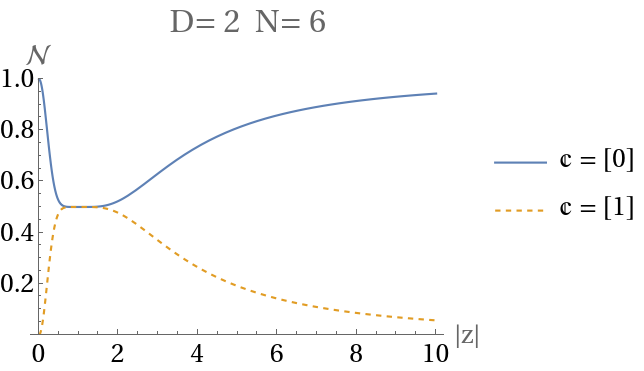
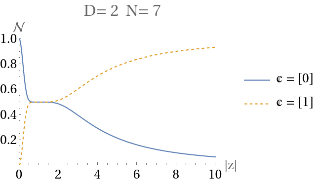
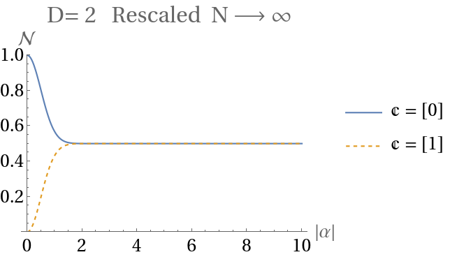
Figure 1: Plots of the normalization factor $\mathcal{N}_{\mathbbm{c}}(\bm{z})^{2}$ for $D=2$,   $N=6$ (left), $N=7$ (center) and in the restaled thermodynamic limit (right), for $|z|,|\alpha|\in[0,10]$.

IV.2 Fock coefficients

The coefficients $c_{\vec{n}}(\bm{z})_{\mathbbm{c}}$ of $|\bm{z}\rangle_{\mathbbm{c}}$ in the Fock basis are:

$$c_{\vec{n}}(\bm{z})_{\mathbbm{c}}=\frac{2^{1-D}}{\mathcal{N}_{\mathbbm{c}}(\bm{z})}\sum_{\mathbbm{b}}\chi_{\mathbbm{c}+\mathbbm{n}}(\mathbbm{b})c_{\vec{n}}(\bm{z})=\frac{c_{\vec{n}}(\bm{z})}{\mathcal{N}_{\mathbbm{c}}(\bm{z})}\delta_{\vec{n}_{0}\;{\rm mod}\;2,\mathbbm{c}}\,,$$ (42)

where $\vec{n}_{0}=(n_{1},\ldots,n_{D-1})$ is retrieved from ${\vec{n}}$ by removing $n_{0}$. With this expression of the Fock coefficients for $|\bm{z}\rangle_{\mathbbm{c}}$, the squared norm can be rewritten as

$$\mathcal{N}_{\mathbbm{c}}(\bm{z})^{2}=\sum_{\|\vec{n}\|_{1}=N}\delta_{\vec{n}_{0}\;{\rm mod}\;2,\mathbbm{c}}|c_{\vec{n}}(\bm{z})|^{2}$$ (43)

Thus, parity adapted $U(D)$-spin CS $|\bm{z}\rangle_{\mathbbm{c}}$ in Eq. (33) contain only basis Fock states $|{\vec{n}}\rangle$ with the same parity as $\mathbbm{c}$ (in the indices $i=1,\ldots,D-1$).

Due to these properties, parity adapted CS can be considered multicomponent Schrödinger cat states, being an extension to $D$ levels and parity $\mathbbm{c}\in\mathbb{Z}_{2}^{D-1}$ of $SU(2)$ Schrödinger cat states Gerry and Grobe (1997), which in turn are the $SU(2)$ version of the traditional even and odd Schrödinger cat states for one-mode harmonic oscillator Dodonov et al. (1974). They are also the $U(D)$ version (extended to all possible parities) of Schrödinger cat states of the multimode harmonic oscillator Ansari and Man’ko (1994). The $SU(2)$ version of these states are related to spin cat states Huang et al. (2015, 2022); Groiseau et al. (2021); Maleki and Zheltikov (2020), with interesting metrological properties. We shall call them “$\mathbbm{c}$-${\scriptstyle\mathrm{DCAT}}$s”, or “${\scriptstyle\mathrm{DCAT}}$s” for short when the parity $\mathbbm{c}$ is not relevant.

It is interestig to note that if we consider parity adapted CS but restricted to the total parity subgroup, i.e. the one generated by $\Pi^{\mathbb{0}}=I$ and $\Pi^{\mathbbm{1}}$, the resulting states are the $U(D)$ version of the even and odd multimode (or polychromatic) Schrödinger cat states introduced in Ansari and Man’ko (1994). In this case, the even or odd parity refers to the total parity, i.e, that of the sum $n_{1}+n_{2}+\ldots+n_{D-1}=N-n_{0}$.

Finally, note that due to the equivalence between the set of coherent states and the Bloch projective space, given by Lemma 2 and Proposition 1, we can extend the definitions in this section to the states parametrized by the Bloch projective space and the ITPS obtained from them, i.e. we can define in the obvious way the ($N$-particle states):

$$|\bm{w}^{\mathbbm{b}}\rangle\quad,\quad|\bm{w}\rangle_{\mathbbm{c}}\quad,\quad|\psi^{\mathbbm{b}}\rangle\quad,\quad|\psi\rangle_{\mathbbm{c}}\,,$$ (44)

where $|\psi\rangle$ here stands for $N$ identical copies of the state given in Eq. (6). Note that the parity transformed states $|\bm{w}^{\mathbbm{b}}\rangle$ and $|\psi^{\mathbbm{b}}\rangle$ are $N$-particle ITPS, whereas the parity adapted states $|\bm{w}\rangle_{\mathbbm{c}}$ and $|\psi\rangle_{\mathbbm{c}}$ are finite sums of ITPS.

Also, by Theorem 1, any state $|\Psi\rangle\in{\cal H}_{N}$ (not necessarily an ITPS) can be writen as a finite sum of coherent states. Therefore we can define $|\Psi\rangle^{\mathbbm{b}}$ and $|\Psi\rangle_{\mathbbm{c}}$ as the corresponding finite sums of parity transformed or parity adapted coherent states. Although parity transformations are well defined for any state through its action on Fock states, see eq. (10), for the purpose of the Schmidt decomposition the expansion in terms of coherent states will be useful in order to use the factorization property of parity transformations given in Lemma 19.

IV.3 Limit values for ${\scriptstyle\mathrm{DCAT}}$s at $\mathbf{z}=\mathbf{0}$: Fock-cat states

It could seem that $\mathbbm{c}$-${\scriptstyle\mathrm{DCAT}}$s for parities $\mathbbm{c}\neq\mathbb{0}$ do not exist at $\bm{z}=\mathbf{0}$, in view of the zero vale of the norm of the unnormalized parity adapted states $\Pi_{\mathbbm{c}}|\bm{z}\rangle$ (see Eq. (35) and Fig. 1 for $D=2$). However, if we consider the normalized $\mathbbm{c}$-${\scriptstyle\mathrm{DCAT}}$s states $|\bm{z}\rangle_{\mathbbm{c}}$ in Eq. (33), they are well-behaved at $\bm{z}=\mathbf{0}$, and their Fock coefficients have the expression:

$$\lim_{\bm{z}\rightarrow\mathbf{0}}c_{\vec{n}}(\bm{z})_{\mathbbm{c}}=\delta_{\vec{n}_{0},\mathbbm{c}}\,.$$ (45)

This means that $\mathbbm{c}$-${\scriptstyle\mathrm{DCAT}}$s are Fock states at $z=0$, in particular the ones given by:

$$\lim_{\bm{z}\rightarrow\mathbf{0}}|\bm{z}\rangle_{\mathbbm{c}}=|n_{0}=N-k,{\vec{n}}_{0}=\mathbbm{c}\rangle=|N-k,c_{1},\ldots,c_{D-1}\rangle\,,$$ (46)

with $k=\|\mathbbm{c}\|_{0}$ the number of non-zero components of $\mathbbm{c}$. We shall call these states Fock-cat states, since they are Fock states but sharing many properties with ${\scriptstyle\mathrm{DCAT}}$s, since they are limits of ${\scriptstyle\mathrm{DCAT}}$s when $\bm{z}\rightarrow\mathbf{0}$.

In the thermodynamic limit ($N\rightarrow\infty$), the same result still applies, but now $n_{0}\rightarrow\infty$ in all cases.

In the rescaled thermodynamic limit (the contraction to $D-1$ harmonic oscillators), the result is also similar, but in this case the $\bm{z}\rightarrow\mathbf{0}$ limit is the $(D-1)$-dimensional harmonic oscillator Fock state:

$$\lim_{\bm{z}\rightarrow\mathbf{0}}|\bm{z}\rangle_{\mathbbm{c}}^{\rm HO}=|\mathbbm{c}\rangle=|c_{1},\ldots,c_{D-1}\rangle\,.$$ (47)

IV.4 Limit values for ${\scriptstyle\mathrm{DCAT}}$s when $\|\mathbf{z}\|\rightarrow\infty$

As it can be seen for the case $D=2$ at Fig. 1 (the two leftmost graphics), the norm approaches either zero or one when $\|z\|\rightarrow\infty$. A similar behaviour can be observed for higher values of $D$ at the coordinate axes. This suggests that we should study with detail these limits in order to properly identify these states.

Define the vector $\mathbbm{z}\in\{0,1\}^{D-1}$ such that $\|\mathbbm{z}\|_{0}=1$, i.e. $\mathbbm{z}$ is a unitary vector pointing in the positive direction of one of the coordinate axes in $\mathbb{R}^{D-1}$ (that is, $\mathbbm{z}$ is a particular element of the canonical basis of $\mathbb{R}^{D-1}$). Then the Fock coefficients of the $\mathbbm{c}$-${\scriptstyle\mathrm{DCAT}}$s in the limit along the coordinate axes are given by:

$$\lim_{r\rightarrow\infty}c_{\vec{n}}(r\mathbbm{z})_{\mathbbm{c}}=\delta_{\vec{n}_{0},\mathbbm{c}+(N-\|\mathbbm{c}\|_{0}-N_{\mathbbm{c}})\mathbbm{z}}\,,$$ (48)

with $N_{\mathbbm{c}}=(N-\|\mathbbm{c}\|_{0})\;{\rm mod}\;2$. This means again that $\mathbbm{c}$-${\scriptstyle\mathrm{DCAT}}$s approach Fock states in these limits, in particular the ones given by:

$$\lim_{r\rightarrow\infty}|r\mathbbm{z}\rangle_{\mathbbm{c}}=|N_{\mathbbm{c}},\mathbbm{c}+(N-\|\mathbbm{c}\|_{0}-N_{\mathbbm{c}})\mathbbm{z}\rangle\,,$$ (49)

and thus they are also Fock-cat states.

In some particular cases, depending on the parity of $N$ and on $\mathbb{c}$ and $\mathbb{z}$, the resulting Fock state has all the particles in the same level (i.e. they are ITPS, with no entanglement). For instance, for $D=2$ the resulting Fock state in the limit $|z|\rightarrow\infty$ is $|0,N\rangle$ if $N$ and $\mathbb{c}$ have the same parity. For $D=3$, $\mathbb{c}=[0,0]$, and even $N$, in the limit $\bm{z}\rightarrow(\infty,0)$ the resulting state is $|0,N,0\rangle$ and in the limit $\bm{z}\rightarrow(0,\infty)$ the resulting state is $|0,0,N\rangle$. For $\mathbb{c}=[1,0]$ and odd $N$, in the limit $\bm{z}\rightarrow(\infty,0)$ the resulting state is $|0,N,0\rangle$. For $\mathbb{c}=[0,1]$ and odd $N$, in the limit $\bm{z}\rightarrow(0,\infty)$ the resulting state is $|0,0,N\rangle$. For $\mathbb{c}=[1,1]$, in none of the cases we obtain a Fock state with all the particles in the same level.

It should be noted that $z_{i}\rightarrow\infty$ for some $i=1,\ldots,D-1$ means that the chosen chart (the one for which $z_{0}\neq 0$) is no longer valid since $z_{0}$ turns out to be zero. In this case the chart for which $z_{i}\neq 0$ should be used instead.

Taking into account this fact, the cases $\|\bm{z}\|\rightarrow 0$ and $z_{i}\rightarrow\infty$ for some $i=1,\ldots,D-1$ should stand on the same foot. For instance, the Fock state $|0,\ldots,0,N,0,\ldots,0\rangle$, with the $N$ particles at level $i$, corresponds (in the notation used in Eq. (6)) to $w_{i}=1,w_{j}=0$ for $j\neq i$ and $\mathbbm{c}=\mathbb{0}$ if $N$ is even and $\mathbbm{c}=[0,\ldots,0,1,0,\ldots,0]$ (with a one at position $i$) if $N$ is odd. The other cases can be treated in a similar fashion.

V Entanglement measures

Entanglement implies quantum correlations among the different parts of a multipartite system. We shall restrict to bipartite entanglement of pure states, where different measures of entanglement exist, depending on how non-entangled (separable) states are defined. In Benatti et al. (2020) some definitions of entanglement are introduced, and in the most basic one (Entanglement-I) separable states are identical TPS states (ITPS), thus the only separable states are coherent states, as shown in Prop. 1. In particlar, symmetrized TPS are entangled according to this definition, due to the exchange symmetry.

For other definitions of entanglement, like (Entanglement-V) in Benatti et al. (2020), also known as mode entanglement, separable states are obtained, in the second quantization formalism, by acting on the Fock vacuum with a product of creation operators which act on a different set of modes (or levels). An example of separable states are basis Fock states $|\vec{n}\rangle$, which however are not separable (except in the case when all the particles are in the same level) with respect to Entanglement-I. Also, with respect to Entanglement-V, coherent states are not separable (see, for instance, Calixto et al. (2021b) for U(3) coherent states).

There is an intense debate in the literature about which of the different notions of entanglement is the correct one for indistinguishable particles, in the sense that entanglement could be used as a resource in quantum information, computation, communication or metrology tasks, see Benatti et al. (2020); Morris et al. (2020); Benatti et al. (2021) and references therein.

Without entering in this debate, we shall stick in this paper to the notion of Entanglement-I, which is very common in the literature, and which provides a mathematically consistent notion of entanglement in terms of $M$-particle RDMs (when $N-M$ quDits are traced out) and their corresponding Schmidt coefficients (see Horodecki et al. (2009) and references therein). We shall use entropic measures on the RDMs to quantify the entanglement (see Wang and Mølmer (2002) for the case of qubits). From the physical (and also the mathematical) point of view, this is justified since we shall work only with CS and finite sums of them. Also, in certain situations, like quDit loss (see Sec. VIII.2), the process of losing one or more quDits is modelled by tracing out by these quDits, and our decomposition fits in perfectly in this scheme.

Since the computation of many entropies (like von Neumann entropy) requires the knowledge of the eigenvalues of the RDM, we shall mainly focus on computing the eigenvalues of these $M$-particle RDMs.

By the Schmidt decomposition theorem (see Horodecki et al. (2009)) the nonzero eigenvalues (the squares of the so called Schmidt coefficients) of the $M$-particle RDM coincide with those of the $(N-M)$-particle RDM, thus we shall restrict to $1\leq M\leq\lfloor\frac{N}{2}\rfloor$. Only in the study of robustness (see Sec. VIII.2) we will be interested in the $(N-M)$-particle RDM.

Starting with a pure state $|\psi\rangle^{(N)}$ in the symmetric irreducible representation of $U(D)$ with $N$ particles/quDits, we define the $M$-particle RDM as:

$$\rho^{(M)}={\rm Tr}_{N-M}|\psi\rangle\langle\psi|^{(N)}\,.$$ (50)

Due to the symmetry of the original state $|\psi\rangle^{(N)}$, the resulting density matrix $\rho^{(M)}$ lies in the symmetric irreducible representation of $U(D)$ with $M$ particles.

VI Schmidt decomposition of DCATs

In this section we provide the main results of the paper on Schmidt decomposition of ${\scriptstyle\mathrm{DCAT}}$s under the bipartition in $M$ and $N-M$ particles, with $1\leq M\leq\lfloor\frac{N}{2}\rfloor$.

VI.1 Decomposition of definite parity projection operators

The following Lemma will be of extreme importance in the following results about Schmidt coefficients of reduced density matrices for states with definite parity, stating that projectors $\Pi_{\mathbbm{c}}$ onto subspaces of definite parity $\mathbbm{c}$ for a given number of particles can be decomposed as a sum over all possible parities of tensor products of projectors on subspaces of definite parity with smaller number of particles.

Lemma 3.

Let $N,M$ integers with $N>1$ and $1\leq M\leq\lfloor\frac{N}{2}\rfloor$. Then:

$$\Pi_{\mathbbm{c}}^{(N)}=\sum_{\mathbbm{c}^{\prime}}\Pi_{\mathbbm{c}-\mathbbm{c}^{\prime}}^{(N-M)}\otimes\Pi_{\mathbbm{c}^{\prime}}^{(M)}=\sum_{\mathbbm{c}^{\prime}}\Pi_{\mathbbm{c}-\mathbbm{c}^{\prime}}^{(M)}\otimes\Pi_{\mathbbm{c}^{\prime}}^{(N-M)}=\sum_{\mathbbm{c}^{\prime}}\Pi_{\mathbbm{c}^{\prime}}^{(N-M)}\otimes\Pi_{\mathbbm{c}-\mathbbm{c}^{\prime}}^{(M)}\,.$$ (51)

Proof: The proof is obvious using Convolution Theorem for $\mathbb{Z}_{2}^{D-1}$:

$$\Pi_{\mathbbm{c}}^{(N)} = 2^{1-D}\sum_{\mathbbm{b}}\chi_{\mathbbm{c}}(\mathbbm{b})\Pi^{\mathbbm{b}(N)}=2^{1-D}\sum_{\mathbbm{b}}\chi_{\mathbbm{c}}(\mathbbm{b})\left(\Pi^{\mathbbm{b}(N-M)}\otimes I^{(M)}\right)\left(I^{(N-M)}\otimes\Pi^{\mathbbm{b}(M)}\right)$$

$$= \sum_{\mathbbm{c}^{\prime}}\left(\Pi_{\mathbbm{c}-\mathbbm{c}^{\prime}}^{(N-M)}\otimes I^{M}\right)\left(I^{(N-M)}\otimes\Pi_{\mathbbm{c}^{\prime}}^{(M)}\right)=\sum_{\mathbbm{c}^{\prime}}\Pi_{\mathbbm{c}-\mathbbm{c}^{\prime}}^{(N-M)}\otimes\Pi_{\mathbbm{c}^{\prime}}^{(M)}\,,$$

where we have used Lemma 19 to factorize $\Pi^{\mathbbm{b}(N)}$:

$$\Pi^{\mathbbm{b}(N)} = \Pi_{1}^{b_{1}}\dots\Pi_{D-1}^{b_{D-1}}=\exp(\mathrm{i}\pi\sum_{j=1}^{D-1}b_{j}S_{jj}^{(N)})=\exp(\mathrm{i}\pi\sum_{j=1}^{D-1}b_{j}(S_{jj}^{(N-M)}\otimes I^{(M)}+I^{(N-M)}\otimes S_{jj}^{(M)}))$$

$$= \exp(\mathrm{i}\pi\sum_{j=1}^{D-1}b_{j}S_{jj}^{(N-M)}\otimes I^{(M)})\exp(\mathrm{i}\pi b_{j}I^{(N-M)}\otimes S_{jj}^{(M)})=\left(\Pi^{\mathbbm{b}(N-M)}\otimes I^{(M)}\right)\left(I^{(N-M)}\otimes\Pi^{\mathbbm{b}(M)}\right)\,,$$

together with the fact that the number operators $S_{jj}$ commute among them for all values of $j$.$\blacksquare$

Note the symmetry under the interchange $(N-M)\leftrightarrow M$, due to the Schmidt Theorem, and the symmetry under the interchange $(\mathbbm{c}-\mathbbm{c}^{\prime})\leftrightarrow\mathbbm{c}^{\prime}$, due to the Convolution Theorem.

VI.2 Decomposition of parity adapted CS

Using the previous result applied to a coherent state we obtain the main result of this paper:

Theorem 3.

Let $N,M$ integers with $N>1$ and $1\leq M\leq\lfloor\frac{N}{2}\rfloor$. Then the $\mathbbm{c}$-${\scriptstyle\mathrm{DCAT}}$ of $N$ particles can be decomposed in terms of superpositions of tensor products of ${\scriptstyle\mathrm{DCAT}}$s of $M$ and $N-M$ particles as:

$$|\bm{z}\rangle_{\mathbbm{c}}^{(N)}=\sum_{\mathbbm{c}^{\prime}}l_{\mathbbm{c},\mathbbm{c}^{\prime}}^{N,M}(\bm{z})|\bm{z}\rangle_{\mathbbm{c}-\mathbbm{c}^{\prime}}^{(N-M)}\otimes|\bm{z}\rangle_{\mathbbm{c}^{\prime}}^{(M)}\,,$$ (54)

with Schmidt coefficients

$$l_{\mathbbm{c},\mathbbm{c}^{\prime}}^{N,M}(\bm{z})=\frac{\mathcal{N}_{\mathbbm{c}-\mathbbm{c}^{\prime}}^{(N-M)}(\bm{z})\mathcal{N}_{\mathbbm{c}^{\prime}}^{(M)}(\bm{z})}{\mathcal{N}_{\mathbbm{c}}^{(N)}(\bm{z})}\,.$$ (55)

Proof: The proof is obvious by applying the previous Lemma and restoring the normalization of the diverse ${\scriptstyle\mathrm{DCAT}}$s appearing in the equation.$\blacksquare$

The Schmidt eigenvalues of the RDM obtained after tracing out $N-M$ particles are given by the squares of the Schmidt coefficients:

$$\lambda_{\mathbbm{c},\mathbbm{c}^{\prime}}^{N,M}(\bm{z})=\left(l_{\mathbbm{c},\mathbbm{c}^{\prime}}^{N,M}(\bm{z})\right)^{2}\,.$$ (56)

Note that the Schmidt eigenvalues depend only on the absolute values $|z_{i}|\,,\,i=1,\ldots,D-1$, and do not depend on the relative phases. They are also invariant under the simultaneous interchange of $(N-M)\leftrightarrow M$ and $(\mathbbm{c}-\mathbbm{c}^{\prime})\leftrightarrow\mathbbm{c}^{\prime}$.

The $M$-particle RDMs are well-defined density matrices, since the eigenvalues are positive and their sum is one.

Proposition 2.

The trace of the $M$-particle RDM $\rho_{\mathbbm{c}}^{(M)}(\bm{z})$ of a $\mathbbm{c}$-${\scriptstyle\mathrm{DCAT}}$ is:

$${\rm Tr}\;\rho_{\mathbbm{c}}^{(M)}(\bm{z})={\rm Tr}\;\left({\rm Tr}_{N-M}{}^{(N)}|\bm{z}\rangle_{\mathbb{c}\;\mathbb{c}}\langle\bm{z}|^{(N)}\right)=\sum_{\mathbbm{c}^{\prime}}\lambda_{\mathbbm{c},\mathbbm{c}^{\prime}}^{N,M}(\bm{z})=1\,.$$ (57)

Proof: Using the definition of the Schmidt numbers, it is easily proven that

$$\sum_{\mathbbm{c}^{\prime}}\lambda_{\mathbbm{c},\mathbbm{c}^{\prime}}^{N,M}(\bm{z}) = \frac{1}{\left(\mathcal{N}_{\mathbbm{c}}^{(N)}(\bm{z})\right)^{2}}\sum_{\mathbbm{c}^{\prime}}\left(\mathcal{N}_{\mathbbm{c}-\mathbbm{c}^{\prime}}^{(N-M)}(\bm{z})\mathcal{N}_{\mathbbm{c}^{\prime}}^{(M)}(\bm{z})\right)^{2}=\frac{1}{\left(\mathcal{N}_{\mathbbm{c}}^{(N)}(\bm{z})\right)^{2}}2^{1-D}\sum_{\mathbbm{b}}\chi_{\mathbbm{c}}(\mathbbm{b})\langle\bm{z}|\bm{z}^{\mathbbm{b}}\rangle^{(N-M)}\langle\bm{z}|\bm{z}^{\mathbbm{b}}\rangle^{(M)}$$ (58)

$$= \frac{1}{\left(\mathcal{N}_{\mathbbm{c}}^{(N)}(\bm{z})\right)^{2}}2^{1-D}\sum_{\mathbbm{b}}\chi_{\mathbbm{c}}(\mathbbm{b})\langle\bm{z}|\bm{z}^{\mathbbm{b}}\rangle^{(N)}=1\,,$$

where Convolution Theorem for $\mathbb{Z}_{2}^{D-1}$ has been used again in the second line.$\blacksquare$

It could seem that the Schmidt decomposition provided by Eq. (54) is ill-defined since the right-hand side of the equation is not invariant under particle permutations. However, it is easy to show that, due to the group-theoretical properties of parity adapted CS, it is in fact symmetric, guaranteeing that the standard Schmidt decomposition for distinguishable bipartite systems works in our case without the need of modification (see for instance the modification suggested in Sciara et al. (2017) for the case of two indistinguishable qubits).

VI.3 Schmidt rank of DCATs

Although there are $2^{D-1}$ terms in the decomposition of a parity adapted CS, not all the eigenvalues $\lambda_{\mathbbm{c},\mathbbm{c}^{\prime}}^{N,M}$ are in general different from zero. There are some general bounds on the rank that we should take into account:

• If some $z_{i}=0$ in eq. (21) $\Rightarrow$ the number of eigenvalues is reduced in a factor 2 if $c_{i}=0$ (see Sec. VII.3)
  Thus, the minimum Schmidt number (attained when $\bm{z}\rightarrow\bm{0}$) is $2^{k}$, with $k=\|\mathbbm{c}\|_{0}$ the number of non-zero components of the vector $\mathbbm{c}$.

• For a given $M$, the dimension of the symmetric representation with $M$ particles is $\tbinom{M+D-1}{M}$.

From this considerations, the next Corollary follows.

Corollary 1.

The Schmidt number of the $M$-particle RDM, defined as the rank of $\rho_{\mathbbm{c}}^{(M)}(\bm{z})$, for a $\mathbbm{c}$-${\scriptstyle\mathrm{DCAT}}$ satisfy the bounds:

$${\rm rank}(\rho_{\mathbbm{c}}^{(M)}(\bm{z}))=\min\{2^{\|\bm{z}\|_{0}+\|\mathbbm{c}_{\mathbb{0}}\|_{0}},\tbinom{M+D-1}{M}\}\,,$$ (59)

with $\|\bm{z}\|_{0}\leq D-1$ the number of non-zero entries of the vector $\bm{z}$, and where $\|\mathbbm{c}_{\mathbb{0}}\|_{0}$ is the number of nonzero entries of the vector $\mathbbm{c}_{\mathbb{0}}$, defined as the subset of components of $\mathbbm{c}$ whose indices coincide with the indices of the zero components of $\bm{z}$.

In Table 1 some examples for the different dimensions are shown, indicating in red the cases where the dimension of the symmetric representation with $M$ particles is smaller than the maximum number of ${\scriptstyle\mathrm{DCAT}}$s.

	Full tensor product $D^{M}$	Symmetric irrep $\tbinom{M+D-1}{M}$	Maximum number of ${\scriptstyle\mathrm{DCAT}}$s $2^{D-1}$
$D=2,M=1$	2	2	2
$D=3,M=1$	3	3	4
$D=3,M=2$	9	6	4
$D=4,M=1$	4	4	8
$D=4,M=2$	16	10	8
$D=5,M=1$	5	5	16
$D=5,M=2$	25	15	16
$D=5,M=3$	125	35	16

Table 1: Dimensions of the full tensor product space ${\cal H}_{1}^{\otimes M}$ and the symmetric representation space ${\cal H}_{M}$ compared with the maximun number of ${\scriptstyle\mathrm{DCAT}}$s, for different values of $D$ and $M$. Red colors refer to cases where the maximum number of ${\scriptstyle\mathrm{DCAT}}$s exceeds the dimension of ${\cal H}_{M}$.

As it can be seen, in general, for $D=2$ (qubits) it is enough to consider 1-particle RDMs to account for the two possible ${\scriptstyle\mathrm{2CAT}}$s (even and odd). For $D=3$ (qutrits) we need 2-particle RDMs to have enough room to accomodate the four ${\scriptstyle\mathrm{3CAT}}$s, and for $D=5$ it is necessary to use 3-particle RDMs to have room for the sixteen ${\scriptstyle\mathrm{5CAT}}$s. Since $2^{D-1}$ grows exponentially with $D$, whereas the binomial coefficient $\tbinom{M+D-1}{M}$ grows as a polynomial of degree $M$ in $D$, if we fix $M$, clearly the number of ${\scriptstyle\mathrm{DCAT}}$s will exceed the maximun rank of the RDMs as $D$ grows. We need to increase also $M$ to have enough room for all possible ${\scriptstyle\mathrm{DCAT}}$s in the RDMs.

From the previous discussion, we can compute the Schmidt rank, i.e. the maximun Schmidt number for all possible $M$-RDM.

Corollary 2.

The Schmidt rank of a $\mathbbm{c}$-${\scriptstyle\mathrm{DCAT}}$ is:

$$\hbox{Schmidt rank of }|\bm{z}\rangle_{\mathbbm{c}}=\max_{1\leq M\leq\lfloor\frac{N}{2}\rfloor}{\rm rank}(\rho_{\mathbbm{c}}^{(M)}(\bm{z}))=2^{\|\bm{z}\|_{0}+\|\mathbbm{c}_{\mathbb{0}}\|_{0}}\leq 2^{D-1}\,.$$ (60)

VI.4 $M$-wise Entanglement entropy of parity adapted $U(D)$-spin coherent states

The knowledge of the Schmidt coefficients and eigenvalues allows to easily compute the Linear and von Neumann entropies

$$\mathcal{L}(\rho)=\frac{d}{d-1}(1-Tr(\rho^{2}))\,,\qquad\mathcal{S}(\rho)=-Tr(\rho\log_{d}\rho)$$ (61)

of the $M$-wise RDM matrices, with $d$ a suitable dimension to normalize the entropies between 0 and 1.

In our case the chosen dimensions (according to the dimension of the symmetric representation for $M$ particles, when $M$ is finite, and to the maximum rank of the RDM for parity adapted CS) are:

$$d=\left\{\begin{array}[]{lcr}\tbinom{M+D-1}{M}&,&\qquad\hbox{finite }\,M\,,\\ \\ 2^{D-1}&,&\hbox{ infinite }\,M\,.\end{array}\right.$$ (62)

In Sec. IX (and in the Supplementary Material) we shall show different plots of von Neumann entropy (line plots for $D=2$, contour plots for $D=3$, angular plots with $\|\bm{z}\|_{2}=R$ for $D=4$ and information diagrams for arbitrary values of $D$). In these plots we shall observe the main features of the entropy of the $M$-wise RDM of parity adapted CS, and therefore of the entanglement of these states.

VII Some interesting limits of the Schmidt eigenvalues

In this section we shall analyse with detail the behaviour of the Schmidt eigenvalues under certain limits ($N\rightarrow\infty$, $M\rightarrow\infty$, $\|\bm{z}\|\rightarrow 0$, $z_{i}\rightarrow 1$, $\|\bm{z}\|\rightarrow\infty$, etc.). We shall make use of the limit values of the normalization factors ${\cal N}_{\mathbbm{c}}(\bm{z})$ computed in Sec. IV.

VII.1 Single thermodynamic limit

In many-body systems, the thermodynamic limit is the limit where the number of particles $N$ grows to infinity. The limit $N\rightarrow\infty$ of the Schmidt eigenvalues has the expression:

$$\lim_{N\rightarrow\infty}\lambda_{\mathbbm{c},\mathbbm{c}^{\prime}}^{N,M}(\bm{z})=\left(\mathcal{N}_{\mathbbm{c}^{\prime}}^{(M)}(\bm{z})\right)^{2}\,.$$ (63)

It turns out that, in this limit, the Schmidt eigenvalues do not depend on the original parity $\mathbbm{c}$, therefore all $\mathbbm{c}$-${\scriptstyle\mathrm{DCAT}}$s have the same Schmidt decomposition in the thermodynamic limit. Thus, looking at the RDMs, we cannot infer the parity of the original state in this limit. This confers an universal character to the thermodynamic limit of the Schmidt decomposition, erasing all information about the parity $\mathbbm{c}$ of the original state.

VII.2 Double thermodynamic limit

Another interesting limit is the double thermodynamic limit, when both $N$ and $M$ go to infinity independently. However, this limit is not well-defined. In fact only one of the iterated limits makes sense (since $M\leq N$). The only possible iterated double thermodynamic limit is:

$$\lim_{M\rightarrow\infty}\lim_{N\rightarrow\infty}\lambda_{\mathbbm{c},\mathbbm{c}^{\prime}}^{N,M}(\bm{z})=2^{-k}\delta_{\mathbbm{c}_{0},\mathbbm{c}^{\prime}_{0}}\,,$$ (64)

where $k=\|\bm{z}\|_{0}$ is the number of nonzero components of the vector $\bm{z}$, and $\mathbbm{c}_{0}$ indicates the subset of components of $\mathbbm{c}$ whose indices coincide with the indices of the zero components of $\bm{z}$.

This shows that the $\infty$-RDM of an infinite number of quDits corresponds to a maximally mixed state of dimension $2^{k}$.

We can also consider the rescaled directional double thermodynamic limit, where both $N$ and $M$ go to infinity but with $M/N=1-\eta$ fixed, and simultaneously the variable $\bm{z}$ is rescaled by $\sqrt{N}$:

$$\lim_{\stackrel{{\scriptstyle N\rightarrow\infty}}{{M=(1-\eta)N}}}\lambda_{\mathbbm{c},\mathbbm{c}^{\prime}}^{N,M}(\bm{\alpha}/\sqrt{N})=\prod_{i=1}^{D-1}\lambda^{HO,\eta}_{c_{i},c^{\prime}_{i}}(\alpha_{i})$$ (65)

with

$$\lambda^{HO,\eta}_{c,c^{\prime}}(\alpha)=\left(\frac{\mathcal{N}_{c-c^{\prime}}^{HO}(\sqrt{\eta}\alpha)\mathcal{N}_{c^{\prime}}^{HO}(\sqrt{1-\eta}\alpha)}{\mathcal{N}_{c}^{HO}(\alpha)}\right)^{2}$$ (66)

with $\eta\in[\frac{1}{2},1)$. Using the expression of $\mathcal{N}_{c}^{HO}(\alpha)$ given in Sec. IV, we arrive at:

$$\lambda^{HO,\eta}_{c,c^{\prime}}(\alpha)=\frac{{\rm exp}_{c-c^{\prime}}(\eta|\alpha|^{2}){\rm exp}_{c^{\prime}}((1-\eta)|\alpha|^{2})}{{\rm exp}_{c}(|\alpha|^{2})}=\frac{1}{2}+(-1)^{c-c^{\prime}}\frac{{\rm exp}_{c}((1-2\eta)|\alpha|^{2})}{2{\rm exp}_{c}(|\alpha|^{2})}\,.$$ (67)

Note that for $\eta=\frac{1}{2}$ we have $\lambda^{HO,\frac{1}{2}}_{1,c^{\prime}}(\alpha)=\frac{1}{2}$ (the odd cat state is maximally entangled for all non-zero values of $\alpha$), and for $\eta\rightarrow 1$ we have

$$\lim_{\eta\rightarrow 1}\lambda^{HO,\eta}_{c,c^{\prime}}(\alpha)=\delta_{c^{\prime},0}\,,$$ (68)

indicating that the fidelity with respect to the original state approaches 1 as $\eta\rightarrow 1$ (see Sec. VIII.2).

This represents a generalization to higher dimensions of the results of Glancy and de Vasconcelos (2008) (see also van Enk and Hirota (2000) for the case $\eta=\frac{1}{2}$), for decoherence of a Schrödinger cat state of the harmonic oscillator (realized with a laser beam) by photon absorption modelled by the passage through a beam splitter of transmisivity $\eta$.

This suggests that in the case of ${\scriptstyle\mathrm{DCAT}}$s, the Schmidt decomposition we have obtained can be physically interpreted as a decoherence process under the loss of $M$-quDits. In this sense, our results can help in designing quantum systems robust under quDit loss, for instance in quantum error correction protocols (see Stricker et al. (2020); Zangi and Qiao (2021) for the case of qubit loss). We shall further discuss this point in Section VIII.2.

VII.3 Limits when $\|\mathbf{z}\|\rightarrow 0$, $|z_{i}|\rightarrow 1$, $\|\mathbf{z}\|\rightarrow\infty$

In this subsection we shall consider diverse limits of the Schmidt eigenvalues in the variable $\bm{z}$.

The limit at $\bm{z}=\bm{0}=(0,0,\ldots,0)$ is important since it will provide the minimum rank of the RDM. It general its expression is cumbersome and we will only give the cases $D=2$ and $D=3$.

For $D=2$ we have:

$$\lim_{z\rightarrow 0}\lambda_{c,c^{\prime}}^{N,M}(z)=\frac{M}{N}\delta_{c,c^{\prime}}+\frac{N-M}{N}\delta_{c^{\prime},0}\,.$$ (69)

Thus at $z=0$ the Schmidt rank is 1 (pure state) for the completely even ($c=0$) ${\scriptstyle\mathrm{2CAT}}$ and 2 for the even case ($c=1$) ${\scriptstyle\mathrm{2CAT}}$. Note that this last statement should be understood in the limit sense since for $c\neq 0$ the action of the parity projector onto the highest state (which lies in the completely even subspace) is zero, $\Pi_{c}|\bm{0}\rangle=0$.

For $D=3$ we have:

$$\lim_{(z_{1},z_{2})\rightarrow(0,0)}\lambda_{[0,0],\mathbbm{c}^{\prime}}^{N,M}(z_{1},z_{2}) = \left(1,0,0,0\right)$$

$$\lim_{(z_{1},z_{2})\rightarrow(0,0)}\lambda_{[0,1],\mathbbm{c}^{\prime}}^{N,M}(z_{1},z_{2}) = \left(\frac{M}{N},\frac{N-M}{N},0,0\right)$$

$$\lim_{(z_{1},z_{2})\rightarrow(0,0)}\lambda_{[1,0],\mathbbm{c}^{\prime}}^{N,M}(z_{1},z_{2}) = \left(\frac{M}{N},0,\frac{N-M}{N},0\right)$$ (70)

$$\lim_{(z_{1},z_{2})\rightarrow(0,0)}\lambda_{[1,1],\mathbbm{c}^{\prime}}^{N,M}(z_{1},z_{2}) = \left(\frac{M(M-1)}{N(N-1)},\frac{M(N-M)}{N(N-1)},\frac{M(N-M)}{N(N-1)},\frac{(N-M)(N-M-1)}{N(N-1)}\right)\,,$$

where at the right-hand side the vector of Schmidt eigenvalues is shown, ordered according to the decimal expression of $\mathbb{c}^{\prime}$. From this expression the rank of the RDM at $\bm{z}=\bm{0}$ is easily obtained and generalized to arbitrary $D$, resulting in a rank equal to $2^{\|\mathbb{c}\|_{0}}$. Note that if some $c_{i}=0$, in the limit $\bm{z}\rightarrow\bm{0}$ the ${\scriptstyle\mathrm{DCAT}}$s with $c_{i}^{\prime}=1$ are absent in the Schmidt decomposition.

The expression we have obtained for the Schmidt eigenvalues in the limit $\bm{z}\rightarrow\bm{0}$ provide the Schmidt decomposition of Fock-cat states appearing in Secs. IV.3 and IV.4.

The limit when $|z_{i}|\rightarrow 1\,,\,i=1,\ldots,D-1$ also deserves attention, since at this point the entropy of the RDM takes its maximum value, as can be checked in the graphs shown in the Supplementary Material. However, the general analytic expression of the limit is cumbersome, therefore we shall consider only some special cases.

For $D=2$ we have:

$$\lim_{|z|\rightarrow 1}\lambda_{c,c^{\prime}}^{N,M}(z)=\frac{1}{2}\,,\qquad\forall c,c^{\prime},\forall N,M,\quad 1\leq M\leq\lfloor\frac{N}{2}\rfloor\,.$$ (71)

Then we conclude that for $D=2$ the RDM is maximally mixed at $|z|=1$.

For $D=3$ we have:

$$\lim_{(|z_{1}|,|z_{2}|)\rightarrow(1,1)} \lambda_{\mathbbm{c},\mathbbm{c}^{\prime}}^{N,M}(\bm{z})=$$

$$\frac{(3^{N-M}+(-1)^{c_{1}-c_{1}^{\prime}}+(-1)^{c_{2}-c_{2}^{\prime}}+(-1)^{c_{1}+c_{2}-c_{1}^{\prime}-c_{2}^{\prime}+N-M})(3^{M}+(-1)^{c_{1}^{\prime}}+(-1)^{c_{2}^{\prime}}+(-1)^{c_{1}^{\prime}+c_{2}^{\prime}+M})}{4(3^{N}+(-1)^{c_{1}}+(-1)^{c_{2}}+(-1)^{c_{1}+c_{2}+N})}\,,$$

$\forall c,c^{\prime},\forall N,M1\quad 1\leq M\leq\lfloor\frac{N}{2}\rfloor$. In particular we have for $M=1$:

$$\lim_{(|z_{1}|,|z_{2}|)\rightarrow(1,1)}\lambda_{\mathbbm{c},[1,1]}^{N,1}(\bm{z})=0\,,\qquad\forall\mathbb{c},\forall N>1\,,$$ (73)

which is due to the fact that ${\cal N}_{[1,1]}(\bm{z})^{(1)}=0\,,\forall\bm{z}\in\mathbb{C}^{2}$. Also, in this case for the other values of $\mathbbm{c}^{\prime}\neq[1,1]$ and $k>1$:

$$\lim_{(|z_{1}|,|z_{2}|)\rightarrow(1,1)}\lambda_{[0,0],\mathbbm{c}^{\prime}}^{2k,1}(\bm{z}) = \frac{1}{3}\,,$$ (74)

$$\lim_{(|z_{1}|,|z_{2}|)\rightarrow(1,1)}\lambda_{[1,1],\mathbbm{c}^{\prime}}^{2k+1,1}(\bm{z}) = \frac{1}{3}\,.$$ (75)

In all other cases the nonzero eigenvalues are practically $\frac{1}{3}$, approaching $\frac{1}{3}$ for large odd $N$. Then we conclude that for $M=1$ the RDM is (approximatelly) maximally mixed when $(|z_{1}|,|z_{2}|)=(1,1)$.

Similar conclusions can be obtained for larger values of $D$, although the expressions are cumbersome. Then we can conclude that at the point $|z_{i}|=1,\,i=1,\ldots,D-1$, the rank of the $M$-wise RDM is ${\rm min}\{\tbinom{M+D-1}{M},2^{D-1}\}$.

The $\|\bm{z}\|\rightarrow\infty$ limit does not exist (except for the case $D=2$, see below), since its value depends on the direction. Using hyper-spherical coordinates in the first hyper-octant, $|z_{i}|=ry_{i}(\vec{\theta})$, $\vec{\theta}\in[0,\frac{\pi}{2}]^{D-2}\,,i=1,2,\ldots D-1$, we can compute the directional limits:

$$\lim_{r\rightarrow\infty}\lambda_{\mathbbm{c},\mathbbm{c}^{\prime}}^{N,M}(r,\vec{\theta})=2^{1-D}\frac{\sum_{\mathbbm{b}}\chi_{\mathbbm{c}-\mathbbm{c}^{\prime}}(\mathbbm{b})Y_{\mathbbm{b}}(\vec{\theta})^{N-M}\sum_{\mathbbm{b}}\chi_{\mathbbm{c}^{\prime}}(\mathbbm{b})Y_{\mathbbm{b}}(\vec{\theta})^{M}}{\sum_{\mathbbm{b}}\chi_{\mathbbm{c}}(\mathbbm{b})Y_{\mathbbm{b}}(\vec{\theta})^{N}}\,,$$ (76)

with $Y_{\mathbbm{b}}(\vec{\theta})=\sum_{i=1}^{D-1}(-1)^{b_{i}}y_{i}(\vec{\theta})^{2}$.

For instance, for $D=3$ we have polar coordinates $Y_{\mathbbm{b}}(\vec{\theta})=(-1)^{b_{1}}\cos^{2}\theta+(-1)^{b_{2}}\sin^{2}\theta$ .

The case $D=2$ deserves special attention, since the limit exists, but care should be taken since in some particular cases undetermined limits can appear. The result is:

$$\lim_{|z|\rightarrow\infty}\lambda_{c,c^{\prime}}^{N,M}(z)=\frac{1}{2}\left[1+\frac{N-M}{N}(-1)^{c^{\prime}+M}+\frac{M}{N}(-1)^{c-c^{\prime}+N-M}\right]\,.$$ (77)

VIII Physical applications

Quantum superpositions of macroscopically distinct quasi-classical states (the so-called Schrödinger cat states) are an important resource for quantum metrology, quantum communication and quantum computation. In particular, superpositions $\frac{1}{2{\cal N}(\alpha)}\left(|\alpha\rangle\pm|e^{{\rm i}\phi}\alpha\rangle\right)$ of harmonic oscillator CS $|\alpha\rangle$ with the same $|\alpha|$ but with different phases (like the even $\phi=0$ and odd $\phi=\pi$ parity adapted CS discussed here) are a common resource in a large variety of experiments (see for instance the encode of a logical qubit in the subspace generated by this kind of superpositions, which is protected against phase-flip errors Grimm et al. (2020); Puri et al. (2019)).

In this section we shall discuss how the ${\scriptstyle\mathrm{DCAT}}$s introduced in this paper can be generated using different Hamiltonians, and how the Schmidt decomposition found here can be usefull to study the interesting problem of quDit loss.

VIII.1 ${\scriptstyle\mathrm{DCAT}}$s generation

In Glancy and de Vasconcelos (2008) different methods of producing optical Schrödinger cats for the harmonic oscillator were discussed, and some of them have been realized experimentally Ourjoumtsev et al. (2006). The experimental creation of optical Schrödinger cat states in cavity QED is discussed in Haroche (1995). A Schrödinger cat state of an ion in a trap has been generated expermentally Monroe et al. (1996), and a Schrödinger cat state formed by two interacting Bose condensates of atoms in different internal states (two-well) has been proposed Cirac et al. (1998). Another proposal is the generation of optomechanical Schrödinger cat states in a cavity Bose-Einstein condensate Li et al. (2022), with a considerable enhancement in the size of the mechanical Schrödinger cat state.

An important tecnique to produce Schrödinger cat states is the use of Kerr o Kerr-like media, like in Grimm et al. (2020); Puri et al. (2019), which allows to create, control and measure a qubit in the subspace generated by various Schrödinger cat states, which is protected against phase-flip errors.

Another Hamiltonian where Schrödinger cat states appear is the Lipkin-Meshkov-Glick (LMG) nuclear model Lipkin et al. (1965). In this case they appear as the ground state solution in the thermodynamic limit, or as approximate solutions for the lowest eigenstates of the Hamiltonian for finite $N$. The LMG model has been also realized in circuit QED scheme Larson (2010), and proposed for optimal state prepration with collective spins Muñoz-Arias et al. (2022).

VIII.1.1 LMG D-Level model

It is surprising that in the literature, when multimode (with $D>2$ modes) systems are considered, the only studied cat states are the ones associated to the total parity subgroup $\mathbb{Z}_{2}\subset\mathbb{Z}_{2}^{D-1}$ (the one formed by the parity transformations in Eqns. (15)-(16), see for instance Dodonov et al. (1995); Fastovets et al. (2021). However, there are models, like the $D$-level LMG model, where the Hamiltonian is invariant under parity transformations, where the lowest energy eigenstate and some of the first excited states are parity adapted CS. More precisely in the limit where the interaction parameter $\lambda\rightarrow\infty$ in the LMG $D$-level model for a finite number of particles, the lowest energy state is approximatelly (with a high fidelity) a completelly even ${\scriptstyle\mathrm{DCAT}}$ with $\bm{z}=(1,1,\ldots,1)$ Calixto et al. (2021a), which corresponds to a maximally entangled state among all parity adapted CS, as was shown in Eqns. (VII.3)-(75). Also, some of the lower excited energy eigenstates are also $\mathbbm{c}$-${\scriptstyle\mathrm{DCAT}}$s with different parities $\mathbbm{c}$.

VIII.1.2 Generation by Kerr-like effect

The optical Kerr effect is a universal technique to generate non-classical states in quantum optics. In Kirchmair et al. (2013) multicomponent Schrödinger cat states were generated in a circuit QED where an intense artifical Kerr effect is created, allowing for single-photon Kerr regime.

In Mirrahimi et al. (2014), a logical qubit is encoded in two or four harmonic oscillator Schrödinger cat states of a microwave cavity, of the form $\frac{1}{2{\cal N}(\alpha)}(|\alpha\rangle\pm|-\alpha\rangle)$ and $\frac{1}{2{\cal N}(\alpha)}(|{\rm i}\alpha\rangle\pm|-{\rm i}\alpha\rangle)$, realizing the $\pi/2$ rotation around the $z$-axis by means of Kerr effect, and exploiting multi-photon driven dissipative processes. A two-photon driven dissipative process is used to stabilize a logical qubit basis of two-component Schrödinger cat states against photon dephasing errors, while a four-photon driven dissipative process stabilizes a logical qubit in four-component Schrödinger cat states, which is protected against single-photon loss.

In Grimm et al. (2020) a logical qubit is created in the subspace of four Schrödinger cat states, $\frac{1}{2{\cal N}(\alpha)}(|\alpha\rangle\pm|-\alpha\rangle)$ and $\frac{1}{2{\cal N}(\alpha)}(|\alpha\rangle\pm{\rm i}|-\alpha\rangle)$, using a Hamiltonian that encompasses both Kerr effect and squeezing in a superconducting microwave resonator. The created qubit is protected under phase-flip errors.

Kerr-like effect in $U(2)$ and $U(D)$ can also be exploited to create Schrödinger cat states, using Hamiltonians of the type $H_{\rm kerr}=\chi J_{z}^{2}$ ($J_{z}=\frac{1}{2}\left(S_{22}-S_{11}\right)$ is the third component of the angular momentum operator) for $SU(2)$ or

$$H_{\rm kerr}=\chi\sum_{j=1}^{D-1}S_{jj}^{2}$$ (78)

for the case of $U(D)$. Note that this Hamiltonian is a particular case of the interacting term of the LMG Hamiltonian for general $D$ Calixto et al. (2021a), which, in the rescaled double thermodinamic limit, approaches the (multimode) Kerr Hamiltonian plus a squeezing term (see Randjbar-Daemi et al. (1993)).

Denoting the revival time as $T_{\rm rev}=\frac{2\pi}{\chi}$, for times $t=T_{\rm rev}/q$, with $q=2,3,\ldots$, this kind of Hamiltonians produce multicomponent Schrödinger cat states, where the number of components is $q$ for odd $q$ and $\frac{q}{2}$ for even $q$ (see Arjika et al. (2019) for the case of $SU(2)$ and the harmonic oscillator).

VIII.2 QuDit loss

A commented in Sec. VII.1, when the rescaled directional double thermodynamic limit was discussed and the results in the literature for the study of photon loss were recovered (and generalized to a larger number or harmonic oscillators, or polycromatic lasers), we can infer that the Schmidt decomposition of parity adapted CS in terms of a sum for all parities of tensor products of parity adapted CS with smaller number of particles, really corresponds to the physical process of quDit loss, when some quDits of a symmetric multi-quDit state are lost by some irreversible process (like decoherence by interaction with the environment or other similar process), and that this process is mathematically described by the partial trace (see, for instance Neven et al. (2018)).

This suggests that in the case of $\mathbbm{c}$-${\scriptstyle\mathrm{DCAT}}$s, the Schmidt decomposition we have obtained can be used to describe a decoherence process under the loss of $M$-quDits. In this sense, our results can help in designing quantum error correction protocols (see Stricker et al. (2020); Zangi and Qiao (2021) for the case of qubit loss).

Our Schmidt decomposition can also be useful in the generalization to quDits of the study of robustness of entanglement under qubit loss Neven et al. (2018). In this context, robustness is defined as the survival of entanglement after the loss of $M$ qubits, i.e. the RDM after tracing out $M$ qubits, $\rho^{(N-M)}_{\,\mathbbm{c}}(\bm{z})$ (which describes in general a mixed state), is entangled.

In our case, as it can be checked in the limit values discussed in Sec. VII and in the Figures in Sec. IX (and in the Supplementary Material), the rank of the RDM is larger than one except possibly in the cases $\|\bm{z}\|\rightarrow 0$ and $|z_{i}|\rightarrow\infty$ (i.e, along some of the axes), and the entropy of the RDM is lower than the NEMSs (Not Entangled Mixed States) limit except in the cases marked in red in Table 1 (changing $M$ by $N-M$), when maximally mixed (not entangled) RDM can appear.

The limits of the ${\scriptstyle\mathrm{DCAT}}$s when $\|\bm{z}\|\rightarrow 0$ and $|z_{i}|\rightarrow\infty$ were studied in Secs. IV.3 and IV.4, and they turn to be Fock states and in some particular cases they are ITPS. Thus, except for the cases where the original state is an ITPS (and therefore it is not entangled), the rank of the resulting RDM is larger than one and $\rho^{(N-M)}_{\,\mathbbm{c}}(\bm{z})$ is entangled (except in the cases marked in red in Table 1).

Therefore, we can guarantee that, except in the mentioned cases, the entanglement of the original ${\scriptstyle\mathrm{DCAT}}$ is robust under quDit loss. This should be compared with the case of GHZ or NOON states, which are maximally entangled but they are fragile under qubit loss Neven et al. (2018). In fact, spin cat states Huang et al. (2015) with moderate entanglement can reach the standard quantum limit even in the presence of a relative large amount of qubit loss, whereas GHZ states lose this capability with an small fraction of qubit loss.

Motivated by the example discussed in van Enk and Hirota (2000); Glancy and de Vasconcelos (2008), where in the case of photon loss when $\eta\rightarrow 1$ the fidelity with the original state approaches one, we would like to introduce the concept of fidelity also in our case. Strictly speaking, the fidelity

$$F_{\mathbbm{c}}^{N,M}(\bm{z})\equiv{}^{(N)}{\!\!\!\!}_{\mathbbm{c}}\langle\bm{z}|\rho^{(N-M)}_{\,\mathbbm{c}}(\bm{z})|\bm{z}\rangle{}^{(N)}_{\mathbbm{c}}\,,$$ (79)

makes sense only in the case $N\rightarrow\infty$, since otherwise the number of particles do not match and the expectation value makes no sense. Alternatively, we can define the fidelity for finite $N$ as:

$$F_{\mathbbm{c}}^{N,M}(\bm{z})\equiv\lambda_{\mathbbm{c},\mathbb{0}}^{N,M}(\bm{z})\,,$$ (80)

i.e., as the component in the Schmidt decompostion where the $(N-M)$ subsystem has the same parity as the original system, and this, according to our definition, corresponds to $\mathbbm{c}^{\prime}=\mathbb{0}$ in Eqn. (54).

This definition of fidelity (and its maximization with respect to $\bm{z}$) could be interesting in some protocols where it is important that the parity $\mathbbm{c}$ of the state should be robust under quDit loss. In other situations, however, it could be interesting the fact that the state has a (quasi) definite parity under quDit loss, without worrying about its value. In this case, $\lambda_{\mathbbm{c},\mathbbm{c}^{\prime}}^{N,M}(\bm{z})$ should be maximized for all possible values of $\mathbbm{c}^{\prime}$, too. And in other situations, it could be interesting to maximize a balanced combination of robustness $+$ fidelity.

IX Figures for $D=2$ atom levels (qubits)

IX.1 Finite number $N$ of qubits

In this section, in Figures 2 ($N=6$) and 3 ($N=7$) we show plots of the normalized von Neumann entropy (see Eq. (61)) of $M$-wise RDMs of the even ($\mathbbm{c}=[0]$) and odd ($\mathbbm{c}=[1]$) $\mathbbm{c}$-${\scriptstyle\mathrm{2CAT}}$ as a function of $|z|$, for values in the range $[0,10]$ . We can observe that all normalized entropies reach the maximum for $|z|=1$, with a value 1, i.e. the ${\scriptstyle\mathrm{2CAT}}$ is maximally entangled, for $M=1$.

In the case of an even number of particles $N$, for the even parity ($\mathbbm{c}=[0]$) ${\scriptstyle\mathrm{2CAT}}$ the entropy is zero (i.e. the ${\scriptstyle\mathrm{2CAT}}$ is a separable pure state) at $z=0$ and for large $|z|$, whereas for the odd ($\mathbbm{c}=[1]$) ${\scriptstyle\mathrm{2CAT}}$ both at $z=0$ and for large $|z|$ the entropy takes the same non-zero value, approaching $\frac{1}{2}$ when $\frac{M}{N}$ approaches $\frac{1}{2}$.

For $N$ odd, the behaviour is similar but the even and odd $\mathbb{c}$ cases get interchanged for large $|z|$.

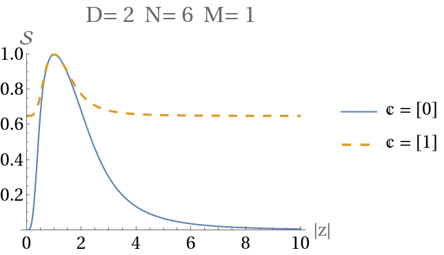
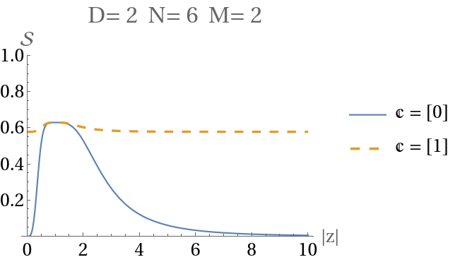
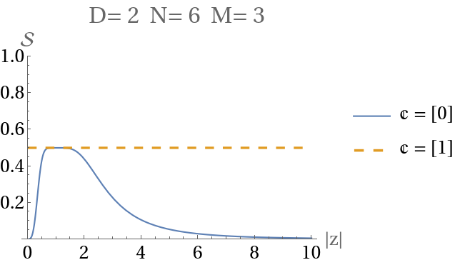
Figure 2: Plots of von Neumann entropy for $D=2,\ N=6$ and $M=1,2,3$, for $|z|\in[0,10]$.

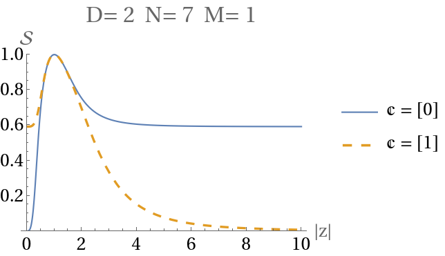
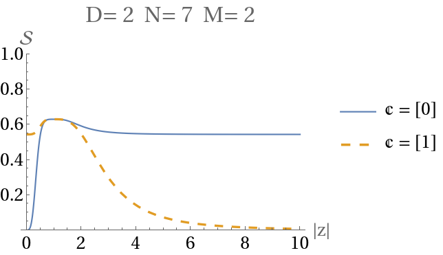
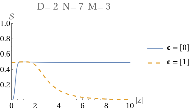
Figure 3: Plots of von Neumann entropy for $D=2,\,N=7$ and $M=1,2,3$, for $|z|\in[0,10]$.

IX.2 Single thermodynamic limit

In this section, in Figure 4 we show plots of the normalized von Neumann entropy of RDMs of the even ($\mathbbm{c}=[0]$) and odd ($\mathbbm{c}=[1]$) $\mathbbm{c}$-${\scriptstyle\mathrm{2CAT}}$ as a function of $|z|$, for values in the range $[0,10]$, in the case $N\rightarrow\infty$. We can observe that all normalized entropies reach the maximum for $|z|=1$, with a value of 1 (i.e. the 2cats are maximally entangled) for $M=1$, and approach zero when $|z|$ approach zero or grows to infinity. In this case the entropies coincide for both parities, agreeing with Eq. (63).

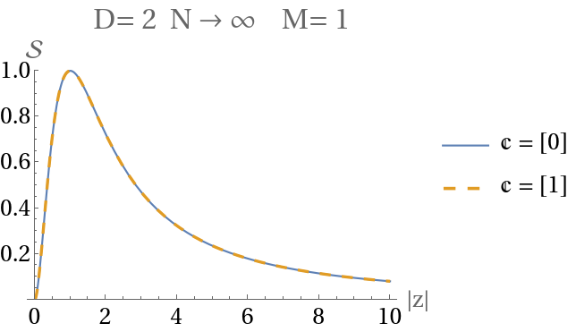
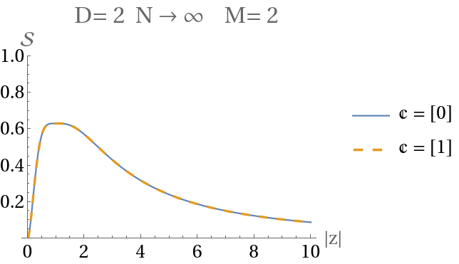
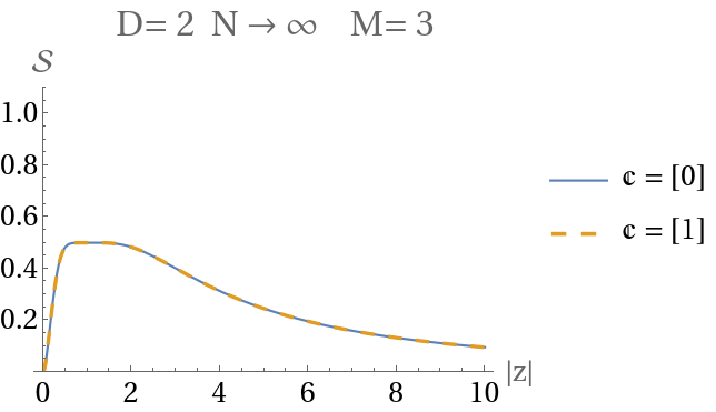
Figure 4: Plots of von Neumann entropy for $D=2,\ N=6$ and $M=1,2,3$, for $|z|\in[0,10]$.

IX.3 Rescaled double thermodynamic limit

Finally, in Figure 5 we show plots of the normalized von Neumann entropy of RDM of the even ($\mathbbm{c}=[0]$) and odd ($\mathbbm{c}=[1]$) $\mathbbm{c}$-${\scriptstyle\mathrm{2CAT}}$ as a function of $|z|$, for values in the range $[0,10]$, in the case $N,M\rightarrow\infty$ with $M=(1-\eta)N$. We can observe that for the even ${\scriptstyle\mathrm{2CAT}}$ the normalized entropy reach the maximum of 1 when $|z|$ grows to infinity, and approach zero when $z$ approach zero. For the odd ${\scriptstyle\mathrm{2CAT}}$, the normalized entropy reach the maximum of 1 when $|z|$ grows to infinity, but approach a non-zero value when $|z|\rightarrow 0$, and this value approach 1 when $\eta$ approach $\frac{1}{2}$, agreeing with the results of Sec. VII.2.

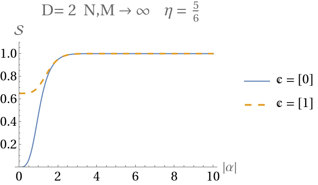
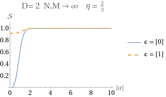
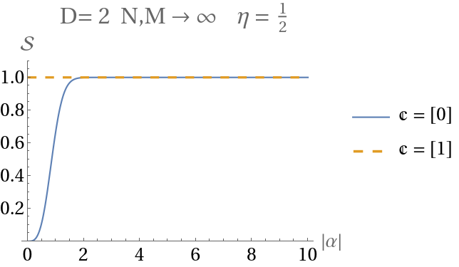
Figure 5: Plots of von Neumann entropy for $D=2,\ N=6$ and $M=1,2,3$, for $|z|\in[0,10]$.

X Conclusions

In this paper we provide a thorough discussion of the entanglement properties of symmetric $N$-quDit systems described by parity adapted CS for $U(D)$ ($\mathbbm{c}$-${\scriptstyle\mathrm{DCAT}}$s), in terms of the entropy of the $M$-wise RDM and proving a Schmidt decomposition theorem under a bipartition of the system in terms of $M<N$ and $N-M$ particles (quDits).

We show that the Schmidt decomposition turns out to be a sum over all possible parities of tensor products of parity adapted CS with smaller number of particles. This Schmidt decomposition is well-defined even though we are treating with indistinguishable particles, the reason being the constraints imposed by the group-theoretical properties of the parity adapted states.

The properties of the Schmidt eigenvalues have been studied for different limit values and different thermodynamic limits, reproducing, in the case of the rescaled double termodynamic limit, known results in the literature for photon loss. This suggests that the obtained Schmidt decomposition and entanglement properties could be useful in designing quantum information and computation protocols with parity adapted CS for quDits of arbitrary $D$, and studying their decoherence properties under quDit loss.

Possible generalizations of this work in different directions are under study. One of them is considering different transformation groups generalizing the parity group $\mathbb{Z}_{2}^{D-1}$, for instance $\mathbb{Z}_{n}^{D-1}$ with $n>2$ (an anisotropic version $\mathbb{Z}_{n_{1}}\times\ldots\mathbb{Z}_{n_{D-1}}$ could also be considered). See Horoshko et al. (2016) for a the particular case of the one-mode harmonic oscillator.

Another possible generalization is to consider mode entanglement instead of particle entanglement, i.e. considering a bipartition of different modes or levels, for instance $D-K$ and $K$, with $0<K<\lfloor\frac{D}{2}\rfloor$. In this case, it is expected that a similar result for the Schmidt decomposition should hold but the decomposition involving parity adapted CS of $U(D-K)$ and $U(K)$. Interlevel entanglement for the case $K=1$ has already been discussed in Calixto et al. (2021b) for $K=1$.

References

- Dicke (1954) R. H. Dicke, “Coherence in spontaneous radiation processes,” Phys. Rev. 93, 99–110 (1954).
- Lipkin et al. (1965) H. J. Lipkin, N. Meshkov, and A. J. Glick, “Validity of many-body approximation methods for a solvable model. (i). exact solutions and perturbation theory,” Nuclear Physics 62, 188–198 (1965).
- Benatti et al. (2020) F. Benatti, R. Floreanini, F. Franchini, and U. Marzolino, “Entanglement in indistinguishable particle systems,” Physics Reports 878, 1–27 (2020).
- Benatti et al. (2021) Fabio Benatti, Roberto Floreanini, and Ugo Marzolino, “Entanglement and non-locality in quantum protocols with identical particles,” Entropy 23 (2021), 10.3390/e23040479.
- Wang and Mølmer (2002) X. Wang and K. Mølmer, “Pairwise entanglement in symmetric multi-qubit systems,” The European Physical Journal D 18, 385–391 (2002).
- Lo Franco and Compagno (2016) Rosario Lo Franco and Giuseppe Compagno, “Quantum entanglement of identical particles by standard information-theoretic notions,” Scientific Reports 6, 20603 (2016).
- Sciara et al. (2017) Stefania Sciara, Rosario Lo Franco, and Giuseppe Compagno, “Universality of schmidt decomposition and particle identity,” Scientific Reports 7, 44675 (2017).
- Killoran et al. (2014) N. Killoran, M. Cramer, and M. B. Plenio, “Extracting entanglement from identical particles,” Phys. Rev. Lett. 112, 150501 (2014).
- Morris et al. (2020) Benjamin Morris, Benjamin Yadin, Matteo Fadel, Tilman Zibold, Philipp Treutlein, and Gerardo Adesso, “Entanglement between identical particles is a useful and consistent resource,” Phys. Rev. X 10, 041012 (2020).
- Guerrero et al. (2022) J. Guerrero, A. Mayorgas, and M. Calixto, “Information diagrams in the study of entanglement in symmetric multi-qudit systems and applications to quantum phase transitions in lipkin–meshkov–glick d-level atom models,” Quant. Inf. Process. 21, 223 (2022).
- Schwinger (1952) J Schwinger, “On angular momentum,” (1952), 10.2172/4389568.
- Dirac (1927) Paul Adrien Maurice Dirac, “The quantum theory of the emission and absorption of radiation,” Proc. R. Soc. Lond. A , 243–265 (1927).
- Fock (1932) V. Fock, “Konfigurationsraum und zweite quantelung,” Zeitschrift für Physik 75, 622–647 (1932).
- Sugita (2003) Ayumu Sugita, “Moments of generalized husimi distributions and complexity of many-body quantum states,” Journal of Physics A: Mathematical and General 36, 9081–9103 (2003).
- Kunz (1979) Kunz, “On the equivalence between one-dimensional discrete walsh-hadamard and multidimensional discrete fourier transforms,” IEEE Transactions on Computers C-28, 267–268 (1979).
- Perelomov (1986) Askold Perelomov, Generalized Coherent States and Their Applications (Springer-Verlag Berlin Heidelberg, 1986).
- Calixto et al. (2021a) Manuel Calixto, Alberto Mayorgas, and Julio Guerrero, “Role of mixed permutation symmetry sectors in the thermodynamic limit of critical three-level Lipkin-Meshkov-Glick atom models,” Phys. Rev. E 103, 012116 (2021a).
- Bengtsson and Zyczkowski (2006) Ingemar Bengtsson and Karol Zyczkowski, Geometry of Quantum States: An Introduction to Quantum Entanglement (Cambridge University Press, 2006).
- Calixto et al. (2021b) Manuel Calixto, Alberto Mayorgas, and Julio Guerrero, “Entanglement and U(D)-spin squeezing in symmetric multi-qudit systems and applications to quantum phase transitions in Lipkin–Meshkov–Glick D-level atom models,” Quantum Information Processing 20, 304 (2021b).
- (20) A. Mayorgas J. Guerrero, A. Sojo and M. Calixto, in preparation .
- Calixto et al. (2008) M. Calixto, J. Guerrero, and J. C. Sánchez-Monreal, “Sampling theorem and discrete Fourier transform on the Riemann sphere,” J. Fourier Anal. Appl. 14, 538–567 (2008).
- Calixto et al. (2011) M. Calixto, J. Guerrero, and J. C. Sánchez-Monreal, “Sampling theorem and discrete fourier transform on the hyperboloid,” J. Fourier Anal. Appl. 17, 240–264 (2011).
- Majorana (1932) Ettore Majorana, “Atomi orientati in campo magnetico variabile,” Il Nuovo Cimento (1924-1942) 9, 43–50 (1932).
- Devi et al. (2012) A. R. Usha Devi, Sudha, and A. K. Rajagopal, “Majorana representation of symmetric multiqubit states,” Quantum Information Processing 11, 685–710 (2012).
- Sanders (1992) Barry C. Sanders, “Entangled coherent states,” Phys. Rev. A 45, 6811–6815 (1992).
- Sanders (2012) Barry C Sanders, “Review of entangled coherent states,” Journal of Physics A: Mathematical and Theoretical 45, 244002 (2012).
- (27) C. Providencia, J. da Providencia, Y. Tsue, and M. Yamamura, “Boson realization of the su(3)-algebra. II: – holstein-primakoff representation for the lipkin model –,” 115, 155–164.
- Randjbar-Daemi et al. (1993) S. Randjbar-Daemi, Abdus Salam, and J. Strathdee, “Generalized spin systems and models,” Phys. Rev. B 48, 3190–3205 (1993).
- Gerry and Grobe (1997) Christopher C. Gerry and Rainer Grobe, “Two-mode su(2) and su(1,1) schrödinger cat states,” Journal of Modern Optics 44, 41–53 (1997), https://doi.org/10.1080/09500349708232898 .
- Dodonov et al. (1974) V.V. Dodonov, I.A. Malkin, and V.I. Man’ko, “Even and odd coherent states and excitations of a singular oscillator,” Physica 72, 597–615 (1974).
- Ansari and Man’ko (1994) N. A. Ansari and V.I. Man’ko, “Photon statistics of multimode even and odd coherent light,” Phys. Rev. A 50, 1942 (1994).
- Huang et al. (2015) Jiahao Huang, Xizhou Qin, Honghua Zhong, Yongguan Ke, and Chaohong Lee, “Quantum metrology with spin cat states under dissipation,” Scientific Reports 5, 17894 (2015).
- Huang et al. (2022) Jiahao Huang, Hongtao Huo, Min Zhuang, and Chaohong Lee, “Efficient generation of spin cat states with twist-and-turn dynamics via machine optimization,” Phys. Rev. A 105, 062456 (2022).
- Groiseau et al. (2021) Caspar Groiseau, Stuart J. Masson, and Scott Parkins, “Generation of spin cat states in an engineered dicke model,” Phys. Rev. A 104, 053721 (2021).
- Maleki and Zheltikov (2020) Yusef Maleki and Aleksei M. Zheltikov, “Spin cat-state family for heisenberg-limit metrology,” J. Opt. Soc. Am. B 37, 1021–1026 (2020).
- Horodecki et al. (2009) Ryszard Horodecki, Paweł Horodecki, Michał Horodecki, and Karol Horodecki, “Quantum entanglement,” Rev. Mod. Phys. 81, 865–942 (2009).
- Glancy and de Vasconcelos (2008) Scott Glancy and Hilma Macedo de Vasconcelos, “Methods for producing optical coherent state superpositions,” J. Opt. Soc. Am. B 25, 712–733 (2008).
- van Enk and Hirota (2000) Steven J. van Enk and Osamu Hirota, “Entangled coherent states: Teleportation and decoherence,” Physical Review A 64, 022313 (2000).
- Stricker et al. (2020) Roman Stricker, Davide Vodola, Alexander Erhard, Lukas Postler, Michael Meth, Philipp Schindler, Thomas Monz, Markus Müller, and Rainer Blatt, “Experimental deterministic correction of qubit loss,” Nature 585, 207–210 (2020).
- Zangi and Qiao (2021) S.M. Zangi and Cong-Feng Qiao, “Robustness of 2xNxM entangled states against qubit loss,” Physics Letters A 400, 127322 (2021).
- Grimm et al. (2020) A. Grimm, N. E. Frattini, S. Puri, S. O. Mundhada, S. Touzard, M. Mirrahimi, S. M. Girvin, S. Shankar, and M. H. Devoret, “Stabilization and operation of a kerr-cat qubit,” Nature 584, 205–209 (2020).
- Puri et al. (2019) Shruti Puri, Alexander Grimm, Philippe Campagne-Ibarcq, Alec Eickbusch, Kyungjoo Noh, Gabrielle Roberts, Liang Jiang, Mazyar Mirrahimi, Michel H. Devoret, and S. M. Girvin, “Stabilized cat in a driven nonlinear cavity: A fault-tolerant error syndrome detector,” Phys. Rev. X 9, 041009 (2019).
- Ourjoumtsev et al. (2006) Alexei Ourjoumtsev, Rosa Tualle-Brouri, Julien Laurat, and Philippe Grangier, “Generating optical schrödinger kittens for quantum information processing,” Science 312, 83–86 (2006), https://www.science.org/doi/pdf/10.1126/science.1122858 .
- Haroche (1995) S. Haroche, “Mesoscopic coherences in cavity qed,” Il Nuovo Cimento B (1971-1996) 110, 545–556 (1995).
- Monroe et al. (1996) C. Monroe, D. M. Meekhof, B. E. King, and D. J. Wineland, “A ”schrödinger cat” superposition state of an atom,” Science 272, 1131–1136 (1996), https://www.science.org/doi/pdf/10.1126/science.272.5265.1131 .
- Cirac et al. (1998) J. I. Cirac, M. Lewenstein, K. Mølmer, and P. Zoller, “Quantum superposition states of bose-einstein condensates,” Phys. Rev. A 57, 1208–1218 (1998).
- Li et al. (2022) Baijun Li, Wei Qin, Ya-Feng Jiao, Cui-Lu Zhai, Xun-Wei Xu, Le-Man Kuang, and Hui Jing, “Optomechanical schrödinger cat states in a cavity bose-einstein condensate,” Fundamental Research (2022), https://doi.org/10.1016/j.fmre.2022.07.001.
- Larson (2010) J. Larson, “Circuit qed scheme for the realization of the lipkin-meshkov-glick model,” Europhysics Letters 90, 54001 (2010).
- Muñoz-Arias et al. (2022) Manuel H. Muñoz-Arias, Ivan H. Deutsch, and Pablo M. Poggi, “Phase space geometry and optimal state preparation in quantum metrology with collective spins,” (2022).
- Dodonov et al. (1995) V. V. Dodonov, V. I. Man’ko, and D. E. Nikonov, “Even and odd coherent states for multimode parametric systems,” Phys. Rev. A 51, 3328–3336 (1995).
- Fastovets et al. (2021) D. V. Fastovets, Yu. I. Bogdanov, N. A. Bogdanova, and V. F. Lukichev, “Schmidt decomposition and coherence of interfering alternatives,” Russian Microelectronics 50, 287–296 (2021).
- Kirchmair et al. (2013) Gerhard Kirchmair, Brian Vlastakis, Zaki Leghtas, Simon E. Nigg, Hanhee Paik, Eran Ginossar, Mazyar Mirrahimi, Luigi Frunzio, S. M. Girvin, and R. J. Schoelkopf, “Observation of quantum state collapse and revival due to the single-photon Kerr effect,” Nature 495, 205–209 (2013).
- Mirrahimi et al. (2014) Mazyar Mirrahimi, Zaki Leghtas, Victor V Albert, Steven Touzard, Robert J Schoelkopf, Liang Jiang, and Michel H Devoret, “Dynamically protected cat-qubits: a new paradigm for universal quantum computation,” New Journal of Physics 16, 045014 (2014).
- Arjika et al. (2019) S. Arjika, M. Calixto, and J. Guerrero, “Quantum statistical properties of multiphoton hypergeometric coherent states and the discrete circle representation,” Journal of Mathematical Physics 60, 103506 (2019), https://doi.org/10.1063/1.5099683 .
- Neven et al. (2018) A. Neven, J. Martin, and T. Bastin, “Entanglement robustness against particle loss in multiqubit systems,” Phys. Rev. A 98, 062335 (2018).
- Horoshko et al. (2016) D. B. Horoshko, S. De Bièvre, M. I. Kolobov, and G. Patera, “Entanglement of quantum circular states of light,” Phys. Rev. A 93, 062323 (2016).