Decarbonization of financial markets:
a mean-field game approach

Abstract

We build a model of a financial market where a large number of firms determine their dynamic emission strategies under climate transition risk in the presence of both green-minded and neutral investors. The firms aim to achieve a trade-off between financial and environmental performance, while interacting through the stochastic discount factor, determined in equilibrium by the investors’ allocations. We formalize the problem in the setting of mean-field games and prove the existence and uniqueness of a Nash equilibrium for firms. We then present a convergent numerical algorithm for computing this equilibrium and illustrate the impact of climate transition risk and the presence of green-minded investors on the market decarbonization dynamics and share prices. We show that uncertainty about future climate risks and policies leads to higher overall emissions and higher spreads between share prices of green and brown companies. This effect is partially reversed in the presence of environmentally concerned investors, whose impact on the cost of capital spurs companies to reduce emissions.

Key words: Decarbonization, climate transition risk large financial markets, equilibrium asset pricing, mean-field games

1 Introduction

Decarbonization of industry is an essential ingredient for a successful environmental transition, and the financial sector has a key role to play in meeting the financing needs of green companies and directing the funds away from brown, carbon intensive projects. The amount of assets invested in climate-aware funds increased more than two-fold in each year between 2018 and 2021, reaching USD 408 billion at the end of 2021 (Morningstar Manager Research, 2022), and several authors aimed to quantify the impact of these additional funding flows on the emission reductions in the real economy. Such impact can be achieved only if green-minded investors target a sufficiently large proportion of companies (Berk and van Binsbergen, 2021), and the environmental performance of each company depends on factors which are not directly controlled by investors, such as the general economic situation, financial health of the company, and future climate policies. The decarbonization of a financial market is therefore the result of interaction of a large number of companies, operating in an uncertain environment, and should be modeled as a dynamic stochastic game with a large number of players.

Here we develop a dynamic model for the decarbonization of a large financial market, arising from an equilibrium dynamics involving companies and investors, and built using the analytical framework of mean-field games. Mean-field games, introduced in Lasry and Lions (2007) and Huang et al. (2006) provide a rigorous way to pass to the limit of a continuum of agents in stochastic dynamic games with a large number of identical agents and symmetric interactions. In the limit, the representative agent interacts with the average density of the other agents (the mean field) rather than with each individual agent. This limiting argument simplifies the problem, leading to explicit solutions or efficient numerical methods for computing the equilibrium dynamics.

The key ingredient of our framework is the notion of mean-field financial market, which describes a large financial market with a continuum of small firms, where the performance of each firm is driven by idiosyncratic noise and a finite number of market-wide risk factors (common noise). We assume that the investors in this market are ’large’ meaning that in every investor’s portfolio the idiosyncratic risk of small firms is completely diversified, and the porfolio value depends only on market-wide risk factors. Consequently, and consistently with the classical finance theories (Ang and Chen, 2007; Jagannathan et al., 1995), only market-wide risk factors are priced, and the stochastic discount factor depends only on the common noise and the ’mean-field’.

We then consider a mean-field market where shares of a continuum of carbon-emitting firms are traded. Each firm determines its dynamic stochastic emission schedule based on its own information and on the market-wide risk factors and market-wide decarbonization dynamics, rather than on the individual decisions of each other small firm, which it cannot observe. To fix its emission level, each firm optimizes a criterion depending on its financial and environmental performance. The financial performance is measured by the market value of the firm’s shares and therefore depends on the stochastic discount factor, introducing an interaction between the firms. The environmental performance is measured by carbon emissions, which are penalized in the optimization functional of the firm. The strength of this emission penalty is stochastic, reflecting the uncertainty of climate transition risk. This “stochastic carbon penalty” is a key feature of our model, allowing us to analyze the impact of climate policy uncertainty on market decarbonization and asset prices in a diffusion setting. We show that even in the absence of green investors, higher uncertainty about future climate policies and transition risks creates incentive for all companies to emit more carbon and leads to higher share prices and higher spreads between share prices of carbon efficient and carbon intensive companies, confirming the findings of De Angelis et al. (2022) in a more realistic setting with stochastic emission schedules.

The second key ingredient of our model is the interaction between two large investors (or two classes of investors), with different views about the future: while the regular investor uses the real-world measure, the green-minded investor uses an alternative measure, which may, for example, overweight the probability of some environmental policies, making the costs of climate transition more material. In the presence of such green-minded investors, all companies will reduce their emissions and pay lower dividends, leading to lower share prices. However, carbon intensive companies are affected much stronger than climate-friendly carbon efficient companies. This pressure on share prices, in turn, spurs the polluting companies to decrease their emissions.

We rigorously prove the existence and uniqueness of the mean-field game Nash equilibrium for the contunuum of firms interacting through market prices of their shares, providing a robust solution to the stochastic “decarbonization game” in a competitive environment. The equilibrium is materialized by the equilibrium stochastic discount factor, which can be used to compute share prices and emission strategies for each firm. We then develop a convergent numerical algorithm to compute the equilibrium and use it to study the impact of climate transition risk and green investors on the market decarbonization dynamics and share prices.

The paper is structured as follows. After discussing the related literature in the remainder of this section, we provide a heuristic description of our approach in the case of a finite number of agents in Section 2. Then, in Section 3, we introduce the notion of mean-field market where large investors may invest into a continuum of firms and in Section 4, we describe the mean-field game setting and define the optimization problem of individual firms and the notion of equilibrium used in this paper. In Section 5, we state and prove the main existence and uniqueness result, propose a convergent numerical algorithm for computing the equilibrium, and prove its convergence to the solution of the mean field game problem is shown. Section 6 illustrates the theory with numerical examples and discusses the implications of our results, and section 7 concludes the paper.

Related literature

Our paper contributes to the emerging literature on impact investing, and on the role of climate risk and uncertainty in sustainable finance. Pástor et al. (2021) build a one-period equilibrium model to describe the impact of investors’ ESG preferences on the performance of green assets. Avramov et al. (2022) analyze the asset pricing implications of the uncertainty of corporate ESG profiles, also in a one-period setting. The impact of sustainable investing on the cost of capital, firm behavior and social outcomes is studied, in a one-period equilibrium model, in an early contribution of Heinkel et al. (2001), and more recently, theoretically and empirically, in (Berk and van Binsbergen, 2021; Oehmke and Opp, 2022; Chowdhry et al., 2019; Landier and Lovo, 2020; Green and Roth, 2021). The impact of climate risk on investors’ choices is also studied in a number of papers. Bolton and Kacperczyk (2021) provide empirical evidence that investors are requiring compensation for their exposure to carbon risk; Ilhan et al. (2021) argue that climate policy uncertainty is priced in the options market, and in particular that cost of downside protection is larger for firms with carbon intensive business models; Bourgey et al. (2022) quantify the impact of carbon emissions on a firm’s credit risk in the context of shared socio-economic pathways, Huang et al. (2018) show that firms adapt their financing choices to physical climate risks affecting their performance; and Krueger et al. (2020) report the results of a survey showing that climate risks are considered to be material by institutional investors, while Andersson et al. (2016), Engle et al. (2020) and Alekseev et al. (2022) develop investment strategies allowing to hedge these risks.

Given that the vast majority of theoretical research on impact investing is done in a one-period setting, De Angelis et al. (2022) develop a continuous-time model for the impact of green investment on company emission dynamics, allowing for time-dependent emission schedules. However, in their model the emissions schedules are deterministic (fixed at time $0$), and the arguments used to prove existence of equilibrium are partly heuristic, because the number of firms is assumed to be finite. In our model the emission schedules are stochastic and the firms can change them at any time depending on their financial performance of the individual company, the market dynamics, and the materialization of climate risk; moreover, the existence and uniqueness of equilibrium is shown rigorously.

Our model is based on the general framework of mean field games introduced in Lasry and Lions (2007) and Huang et al. (2006), and more precisely mean-field games with common noise (Carmona et al., 2016; Carmona and Delarue, 2018b; Cardaliaguet et al., 2019). Mean field game with common noise are often untractable due to the lack of compactness of the space containing the random measures, which correspond to the conditional law of the state process given the common noise. A possible workaround is to discretize the common noise to recover compactness and apply Kakutani’s or Schauder’s fixed point theorem (Carmona et al., 2016; Barrasso and Touzi, 2022). In this paper, instead of working on the space of random measures, we write our mean field game problem as a fixed point equation for the stochastic discount factor (interaction term). The proof strategy is to form a strictly convex minimization problem whose first order condition is equivalent to the fixed point problem. This allows us to show the existence and uniqueness of a strong solution to the mean field game problem and to apply the generalized conditional gradient algorithm (Bredies et al., 2009) to provide a numerical solution.

We also contribute to the literature on equilibrium models based on mean-field games. In mathematical finance, Fujii and Takahashi (2022), Fu et al. (2021), Féron et al. (2022), Gomes et al. (2021) and Casgrain and Jaimungal (2020), among other authors, developed models of equilibrium price formation based on interaction of a large number of traders in the framework of mean-field games. In these models, although market clearing may be imposed, the agents are cost minimizers rather than utility optimizers so that that Arrow-Debreu equilibrium is not constructed. A game of many utility maximizing agents is considered in Lacker and Soret (2020), but the agents are price takers in this reference. Instead, we build on the classical equilibrium approach, along the lines of Duffie and Huang (1985); Duffie (1986); Huang (1987) and many more recent papers (Anderson and Raimondo, 2008; Hugonnier et al., 2012; Riedel and Herzberg, 2013), where utility-optimizing agents determine prices in equilibrium. Although mean-field games and related notions have been used in economics, for example, in industry dynamics models (Luttmer, 2007) and for modeling income and wealth distributions (Achdou et al., 2022) they have rarely been applied in equilibrium pricing theory.

2 Motivation : a $n$-firm financial market model

Although we will be primarily interested in the mean-field game model in this paper, we start by describing the $n$-agent setting to motivate the limit as the number of agents goes to infinity. The discussion in this section is heuristic; precise statements and proofs will be given in the mean-field setting in the subsequent sections.

Consider a sequence of filtered probability spaces $(\Omega^{n},\mathcal{F}^{n},\mathbb{F}^{n},\mathbb{P}^{n})$. We assume that, on each probability space $(\Omega^{n},\mathcal{F}^{n},\mathbb{F}^{n},\mathbb{P}^{n})$, there exists a $d$-dimensional standard Brownian motion $B^{0}$ and an independent $n$-dimensional standard Brownian motion $(B^{1},\dots,B^{n})$. The space $(\Omega^{n},\mathcal{F}^{n},\mathbb{F}^{n},\mathbb{P}^{n})$ describes a financial market with $n$ companies.

Individual firm dynamics and optimization

We assume that the firm value of $i$-th company follows the dynamics below:

$$\mathrm{d}V^{i}_{t}=V^{i}_{t}(\mu^{i}_{t}\mathrm{d}t+\sigma^{i}_{t}\mathrm{d}B^{i}_{t}+\sigma^{i,0}_{t}\mathrm{d}B^{0}_{t})+c^{i}_{t}\psi^{i}_{t}\mathrm{d}t,\quad V^{i}_{0}=v_{i}.$$ (1)

Here, the Brownian motion $B$ models the idiosyncratic risk of the company, while $B^{0}$ corresponds to market-wide and economy-wide risk factors. The process $\psi^{i}_{t}\geq 0$ denotes the instantaneous emissions of firm $i$ and the process $c^{i}_{t}$ is inversely proportional to the emission intensity of production and will be referred to as “emission efficacy” in the sequel; the values of this process are low for carbon-intensive companies and high for green, carbon efficient firms which create a lot of wealth with little emissions. Thus, in the absence of emissions, the firm value follows an autonomous dynamics (with perhaps $\mu^{i}_{t}<0$), and to increase the firm value beyond this baseline, the firm must produce and therefore increase its emissions.

The solution to Equation (1) is given explicitly by

$$V^{i}_{t} =v_{i}\mathcal{E}^{i}_{t}+\mathcal{E}^{i}_{t}\int_{0}^{t}\mathcal{E}^{i,-1}_{s}c^{i}_{s}\psi_{s}\mathrm{d}s,$$

$$\mathcal{E}^{i}_{t} =\exp\left(\int_{0}^{t}\sigma^{i}_{s}\mathrm{d}B^{i}_{s}+\int_{0}^{t}\sigma^{i,0}_{s}\mathrm{d}B^{0}_{s}+\int_{0}^{t}\left(\mu^{i}_{s}-\frac{(\sigma^{i})^{2}}{2}-\frac{(\sigma^{i,0})^{2}}{2}\right)\mathrm{d}s\right).$$

We fix a time horizon $T>0$ and assume, as in many papers on equilibrium asset pricing, that at this time the firm pays to its shareholders a terminal liquidating dividend equal to the firm value $V^{i}_{T}$ per share. To be consistent with the limiting framework, we assume that each company has exactly $1/n$ shares outstanding. Further, we assume the existence of a complete and arbitrage-free financial market, where the shares of all firms are traded, and the prices are determined by a stochastic discount factor process $(\xi^{n}_{t})_{0\leq t\leq T}$ with $\xi^{n}_{0}=1$: the price of $i$-th company’s stock at time $t\leq T$ is given by

$$S^{i}_{t}=\frac{1}{\xi^{n}_{t}}\mathbb{E}[\xi^{n}_{T}V^{i}_{T}|\mathcal{F}_{t}].$$ (2)

Moreover, we assume the existence of a risk-free asset paying zero interest, which means that

$$\xi^{n}_{t}=\mathbb{E}[\xi^{n}_{T}|\mathcal{F}_{t}].$$

This means that it is enough to determine $\xi^{n}_{T}$ and to simplify notation we shall denote $\xi^{n}:=\xi^{n}_{T}$.

To determine its emission schedule, each company aims to optimize the following functional:

$$J^{i}(\psi^{i})=S^{i}_{0}-\frac{1}{2}\mathbb{E}\left[\int_{0}^{T}\alpha^{i}_{t}|\psi^{i}_{t}|^{2}\mathrm{d}t\Big{|}\mathcal{F}_{0}\right].$$

Here, the second term corresponds to direct or indirect costs associated to emissions, and the stochastic process $(\alpha^{i}_{t})_{0\leq t\leq T}$ models the future intensity of such costs. Each company therefore aims to achieve a trade-off between maximizing financial performance, as measured by the share price, and minimizing the negative environmental impact, as measured by the emission penalty. Using equilibrium share price as a measure of financial performance in the optimization objective of the firm is consistent with the literature (Heinkel et al., 2001). De Angelis et al. (2022) suggest to use the expected sum of discounted future prices, but since the price at time $t=0$ already accounts for all future cash flows, it seems sufficient and more natural to use the initial price. On the other hand, convex emission penalty similar to ours was used, for example in the context of a single-firm optimization problem in Bourgey et al. (2022).

Using the formula (2) for the share price, we see that maximizing $J^{i}$ is equivalent to maximizing

$$\mathbb{E}\left[\xi^{n}\mathcal{E}^{i}_{T}\int_{0}^{T}\mathcal{E}^{i,-1}_{t}c^{i}_{t}\psi^{i}_{t}\mathrm{d}t-\frac{1}{2}\int_{0}^{T}\alpha^{i}_{t}(\psi^{i}_{t})^{2}\mathrm{d}t\Big{|}\mathcal{F}_{0}\right].$$

The optimal solution takes the form

$$\psi^{i}_{t}=\frac{c^{i}_{t}}{\alpha^{i}_{t}}\mathbb{E}[\xi^{n}\mathcal{E}^{i}_{t,T}|\mathcal{F}_{t}],$$ (3)

where $\mathcal{E}^{i}_{t,T}=\mathcal{E}^{i,-1}_{t}\mathcal{E}^{i}_{T}$, and the corresponding terminal dividend equals

$$V^{i}_{T}=v_{i}\mathcal{E}^{i}_{T}+\int_{0}^{T}\frac{(c^{i}_{t})^{2}}{\alpha^{i}_{t}}\mathcal{E}^{i}_{t,T}\,\mathbb{E}[\xi^{n}\mathcal{E}^{i}_{t,T}|\mathcal{F}_{t}]\mathrm{d}t.$$ (4)

The financial market

We further assume that in the financial market there are two investors: the green investor and the regular investor. The green investor solves the optimization problem

$$\min_{W^{g}}\mathbb{E}^{n,g}[e^{-\gamma^{g}W^{g}}]\quad\text{subject to}\quad\mathbb{E}^{n}[\xi^{n}W^{g}]\leq w^{g},$$

and the regular investor solves

$$\min_{W^{r}}\mathbb{E}^{n}[e^{-\gamma^{r}W^{r}}]\quad\text{subject to}\quad\mathbb{E}^{n}[\xi^{n}W^{r}]\leq w^{r}.$$

Here, $\mathbb{E}^{n}$ denotes the expectation with respect to the probability measure $\mathbb{P}^{n}$, and $\mathbb{E}^{n,g}$ denotes the expectation with respect to the probability measure of the green investor $\mathbb{P}^{n,g}$, defined by

$$\frac{\mathrm{d}\mathbb{P}^{n,g}}{\mathrm{d}\mathbb{P}^{n}}=Z,\quad Z=e^{-\int_{0}^{T}\lambda_{s}\mathrm{d}B^{0}_{s}-\frac{1}{2}\int_{0}^{T}|\lambda_{s}|^{2}\mathrm{d}s}.$$

The green investor thus solves the optimization problem under a different probability measure, under which, for example, the emission cost parameter $\alpha^{i}_{t}$ may follow a different distribution, making the climate transition risks more material. Note also that the density of the measure change depends only on the market-wide risk factors but not on individual risk of each company, since we aim to study large portfolio investors, who do not have access to private information of each firm.

The solutions to the optimization problems are of the form

$$W^{g}=\frac{1}{\gamma^{g}}\ln\frac{\xi^{n}}{Z}+c^{g},\qquad W^{r}=\frac{1}{\gamma^{r}}\ln{\xi^{n}}+c^{r},$$

for some constants $c^{g}$ and $c^{r}$ to be determined.

The market clearing condition assuming unlimited supply of the risk-free asset writes:

$$W^{r}+W^{g}=\frac{1}{n}\sum_{i=1}^{n}V^{i}_{T}+c,$$

for an arbitrary constant $c$. Solving for the stochastic discount factor, we find:

$$\xi^{n}=\frac{\exp\left(-\gamma^{*}\frac{1}{n}\sum_{i=1}^{n}V^{i}_{T}+\rho\ln Z\right)}{\mathbb{E}\left[\exp\left(-\gamma^{*}\frac{1}{n}\sum_{i=1}^{n}V^{i}_{T}+\rho\ln Z\right)\right]},$$ (5)

where $\rho=\frac{\gamma^{r}}{\gamma^{g}+\gamma^{r}}\in(0,1)$. Since the optimal dividend of each company $V^{i}_{T}$, given by (4) depends on the stochastic discount factor, it is tempting to interpret equation (5) as a fixed-point equation and look for the equilibrium stochastic discount factor. However in the $n$-agent setting, the solution (3) is not optimal in equilibrium, since the stochastic discount factor $\xi^{n}$ depends on the emission strategy of the $i$-th firm. Nevertheless, this fixed-point argument becomes valid in the mean-field game setting that we consider in the rest of this paper. First, in the following section, we define the suitable notion of financial market, where large investors invest into a continuum of small companies.

3 Mean-field financial market

Stochastic context and notations

The following notations shall be used for the rest of this paper. Let $(\Omega,\mathcal{F},\mathbb{P})$ be a probability space, supporting a pair $(B,B^{0})$ of independent (possibly multidimensional) standard Brownian motions and an independent random variable $X$ corresponding to the initial condition. We denote by $\mathbb{F}=(\mathcal{F}_{t})_{t\geq 0}$ the $\mathbb{P}$-complete natural filtration of $(X,B,B^{0})$ and by $\mathbb{F}^{0}=(\mathcal{F}^{0}_{t})_{t\geq 0}$ the $\mathbb{P}$-complete natural filtration of $B^{0}$. In our setting, $B$ is an idiosyncratic noise and $B^{0}$ is the common noise. Following standard mean field game theory, the common noise $B^{0}$ appears in the state equation of the representative firm and captures the intrinsic randomness of the market environment. The expectation with the respect to the reference measure $\mathbb{P}$ will be denoted simply by $\mathbb{E}$, and the expectation with respect to any other measure $\mathbb{Q}$ will be denoted by $\mathbb{E}_{\mathbb{Q}}$.

In general, for a $\sigma$-field $\mathcal{G}$, we denote by $L^{p}(\mathcal{G})$ the space of $\mathcal{G}$-measurable random variables $X$ satisfying

$$\mathbb{E}[|X|^{p}]<+\infty,$$

and for a filtration $\mathbb{G}=(\mathcal{G}_{t})_{0\leq t\leq T}$ we denote by $L^{p}(\mathbb{G})$ the space of $\mathbb{G}$-progressively measurable random processes $(X_{t})_{0\leq t\leq T}$ satisfying

$$\mathbb{E}\left[\int_{0}^{T}|X_{t}|^{p}\mathrm{d}t\right]<+\infty.$$

Similarly, we denote by $L^{0}(\mathcal{G})$ and $L^{0}(\mathbb{G})$ the spaces of measurable random variables and progressively measurable random processes without a specific integrability condition. Moreover, for a $\sigma$-field $\mathcal{G}$ we write

$$L_{+}^{p}(\mathcal{G})=\{X\in L^{p}(\mathcal{G}):X\geq 0\;\text{a.s.}\}.$$

Finally, $\mathds{1}\in L^{p}(\mathcal{F}_{T})$ for all $p$ denotes the constant variable equal to $1$ almost surely.

It is clear that $\mathbb{F}^{0}$ satisfies the immersion property with respect to $\mathbb{F}$ (Carmona and Delarue, 2018a, page 5), which implies, in particular, that for all $\zeta\in L^{1}(\mathcal{F}_{t})$, $\mathbb{E}[\zeta|\mathcal{F}^{0}_{T}]=\mathbb{E}[\zeta|\mathcal{F}^{0}_{t}]$.

Description of the market

In the rest of this section we define the notion of mean-field financial market, needed to study the behavior of large portfolio investors in financial markets with many small companies. We consider a large financial market with a risk-free asset whose price is constant and equal to $1$ and a continuum of risky assets. According to the paradigm of mean-field games, we define the market by means of the representative risky asset, whose price follows the dynamics

$$\frac{\mathrm{d}S_{t}}{S_{t}}=\eta_{t}\mathrm{d}t+\beta_{t}\mathrm{d}B_{t}+\beta^{0}_{t}\mathrm{d}B^{0}_{t},\quad S_{0}\in L^{0}(\mathcal{F}_{0}),$$

where $(\eta_{t})_{t\in[0,T]}$, $(\beta_{t})_{t\in[0,T]}$ and $(\beta^{0}_{t})_{t\in[0,T]}$ belong to $L^{0}(\mathbb{F})$ and are such that

$$\int_{0}^{T}(|\eta_{t}|+|\beta_{t}|^{2}+|\beta^{0}_{t}|^{2})\mathrm{d}t<+\infty\quad\text{a.s.}$$

This process defines simultaneously the dynamics of a single asset and the distribution of prices of all assets in the market at any given time. For example, the law of $S_{t}$ conditional on the common noise, denoted by $m_{t}=\mathcal{L}(S_{t}|\mathcal{F}^{0}_{t})$ defines the distribution of asset prices at time $t$, given the realization of the common factors up to time $t$. The process $(m_{t})_{0\leq t\leq T}$ is a random process, adapted to the filtration of the common noise $\mathbb{F}^{0}$ and taking values in the space of probability measures on $\mathbb{R}_{+}$. Since $m_{t}$ is a probability measure, we implicitly assume that the total quantity of all stocks in the market (the market size) is normalized to $1$.

We assume that there exists a stochastic discount factor process $(\xi_{t})_{0\leq t\leq T}$ with $\xi_{0}=1$ and $\xi_{t}>0$ for all $t\in[0,T]$ a.s., such that

• $(\xi_{t})_{0\leq t\leq T}$ is a $\mathbb{F}^{0}$-martingale;

• $(S_{t}\xi_{t})_{0\leq t\leq T}$ is a $\mathbb{F}$-martingale.

Under the martingality assumption, one can also define the equivalent martingale measure $\mathbb{Q}$ by taking $\mathbb{Q}(A)=\mathbb{E}[\xi_{T}\mathbf{1}_{A}]$ for all measurable sets $A$.

By the martingale representation theorem, and given the positivity of the stochastic discount factor, it can be written in the following form:

$$\xi_{t}=1-\int_{0}^{t}\xi_{s}\theta_{s}\mathrm{d}B^{0}_{s},$$

for some $\mathbb{F}^{0}$-adapted process $\theta$. Applying the integration by parts formula we can write:

$$\mathrm{d}(S_{t}\xi_{t})=S_{t}\xi_{t}(\eta_{t}\mathrm{d}t-\theta_{t}\beta^{0}_{t}\mathrm{d}t+\beta_{t}\mathrm{d}B_{t}+\beta^{0}_{t}\mathrm{d}B^{0}_{t}-\theta_{t}\mathrm{d}B^{0}_{t}),$$

so that $\eta_{t}=\theta_{t}\beta^{0}_{t}$ and we can write the representative risky asset price as follows:

$$\frac{\mathrm{d}S_{t}}{S_{t}}=\beta_{t}\mathrm{d}B_{t}+\beta^{0}_{t}(\theta_{t}\mathrm{d}t+\mathrm{d}B^{0}_{t}).$$

In other words, only common market-wide risk factors have a risk-premium and idiosyncratic risk factors are not priced in this large market since they are fully diversifiable.

A mean-field portfolio strategy is a couple $(V_{0},\phi)$, where $V_{0}\in\mathbb{R}$ is a constant and $\phi$ is a $\mathbb{F}$-adapted $\mathbb{R}$-valued stochastic process $\phi$. In this large market, we assume that in any investor’s portfolio, the idiosyncratic risk of individual stocks is fully diversified. This is consistent with the practices of large portfolio investors who may invest simultaneously in thousands of stocks. Thus, the value of the investor’s portfolio at time $t$ writes:

$$V^{\phi}_{t} :=\mathbb{E}\left[\left.V_{0}+\int_{0}^{t}\phi_{s}\mathrm{d}S_{s}\right|\mathcal{F}^{0}_{t}\right].$$

A mean-field portfolio strategy is admissible if $V^{\phi}$ is bounded below by an $\mathbb{F}^{0}$-martingale at all times. Consequently, we say that a mean-field market is weakly complete if for any contingent claim $H_{T}\in L^{1}(\mathcal{F}^{0}_{T},\mathbb{Q})$ there exists an admissible portfolio strategy $(V_{0},\phi)$ with $V^{\phi}_{T}=H_{T}$. Since we only require the replicability of claims in the filtration of the common noise, weak completeness is in general easier to obtain than standard completeness; on the other hand because of the large degree of redundancy in a mean-field market, the mean-field portfolio strategy replicating a given claim is in general not unique.

If appropriate integrability conditions are satisfied, one can substitute the dynamics of $S$ and compute:

$$V^{\phi}_{T}=V_{0}+\int_{0}^{T}\mathbb{E}\left[\phi_{t}S_{t}\beta^{0}_{t}|\mathcal{F}^{0}_{t}\right](\theta_{t}\mathrm{d}t+\mathrm{d}B^{0}_{t}).$$

Example: Black-Scholes mean-field market

Let $B^{0}$ be of dimension $n$, and assume that $\beta^{0}_{t}$ is a constant random vector: $\beta^{0}_{t}=\beta^{0}\in\mathcal{F}_{0}$, and that it spans the entire space $\mathbb{R}^{n}$, in other words, there exists a random vector $f\in L^{0}(\mathcal{F}_{0})$ such that $\mathbb{E}[\beta^{0}f^{\top}]$ is the identity matrix. This means that the ”common noise” part of stock volatilities is constant in time. By the martingale representation theorem applied under the risk-neutral measure $\mathbb{Q}$ (Revuz and Yor, 2013, paragraph 5.3), for any claim $H_{T}\in L^{1}(\mathbb{F}^{0}_{T},\mathbb{Q})$ there exists an $\mathbb{F}^{0}$-adapted process $\phi^{H}$ with

$$H_{T}=\mathbb{E}_{\mathbb{Q}}[H_{T}]+\int_{0}^{T}\phi^{H}_{t}(\theta_{t}\mathrm{d}t+dB^{0}_{t}).$$

Letting $\phi_{t}=\frac{f^{\top}\phi^{H}_{t}}{S_{t}}$ and $V_{0}=\mathbb{E}_{\mathbb{Q}}[H_{T}]$, it follows that $V^{\phi}_{T}=H_{T}$, thus the market is complete in the sense defined above. Note that we have been able to replicate the claim written on a multidimensional Brownian motion with a one-dimensional representative asset and a one-dimensional portfolio strategy, because the representative asset actually represents many assets (an infinity of them), and the portfolio strategy describes the full distribution of weights over these assets.

4 A mean-field game model of decarbonization

In this section we present the problem under study. This problem can be understood as a limiting game when the number of firms tends to infinity in the above $n$-player game, but we focus directly on the mean-field setting and leave the proof of convergence of the $n$-firm setting to the mean field for subsequent research.

4.1 The representative firm problem

The value of the firm per share is assumed to evolve according to the following stochastic differential equation

$$\mathrm{d}V_{t}=V_{t}(\mu_{t}\mathrm{d}t+\sigma_{t}\mathrm{d}B_{t}+\sigma^{0}_{t}\mathrm{d}B^{0}_{t})+c_{t}\psi_{t}\mathrm{d}t,\quad V_{0}=V$$ (6)

where $V\in L^{0}(\mathcal{F}_{0})$ and $V>0$ almost surely. The processes $(\mu_{t})_{0\leq t\leq T}$, $(\sigma_{t})_{0\leq t\leq T}$, $(\sigma^{0}_{t})_{0\leq t\leq T}$ and $(c_{t})_{0\leq t\leq T}$ are assumed to belong to $L^{0}(\mathbb{F})$ and satisfy

$$\int_{0}^{T}(|\mu_{t}|+|\sigma_{t}|^{2}+|\sigma^{0}_{t}|^{2}+|c_{t}|^{2})\mathrm{d}t<+\infty\quad\text{a.s.}$$

The parameter $\mu$ is real-valued, $\sigma$ and $\sigma^{0}$ are vector-valued of the same dimension as the corresponding Brownian motions, and $c$ takes positive values almost surely.

Each firm controls its value via the control $\psi$ which represents its emission flow. We denote $V^{\psi}$ the solution to the state equation for a given control $\psi$. We define the following stochastic exponential

$$\mathcal{E}_{t}=\exp\left(\int_{0}^{t}\sigma_{s}\mathrm{d}B_{s}+\int_{0}^{t}\sigma^{0}_{s}\mathrm{d}B_{s}^{0}+\int_{0}^{t}(\mu_{s}-\frac{|\sigma_{s}|^{2}}{2}-\frac{|\sigma_{s}^{0}|^{2}}{2})\mathrm{d}s\right),\\$$ (7)

and we denote $\mathcal{E}_{s,t}\coloneqq\mathcal{E}_{t}\mathcal{E}_{s}^{-1}$ for all $0\leq s\leq t\leq T$.

Lemma 1.

For any $\psi$ such that $\int_{0}^{T}\psi_{s}^{2}ds<+\infty$ a.s., the equation (6) has a unique solution given by

$$V^{\psi}_{t}=\mathcal{E}_{t}V+\int_{0}^{t}\mathcal{E}_{s,t}c_{s}\psi_{s}\mathrm{d}s,\quad V^{\psi}_{0}=V.$$ (8)

Proof.

This result follows from (Protter, 2005, Theorem 7, Chapter V) and (Protter, 2005, Theorem 52, Chapter V). ∎

We assume that each firm pays a single liquidating dividend at time $T$, equal to $V^{\psi}_{T}$, per share. For any stochastic discount factor $\xi$, assuming the appropriate integrability conditions are satisfied, the share price of the firm is therefore given by

$$S^{\xi,\psi}_{t}=\frac{1}{\xi_{t}}\mathbb{E}\left[\left.\xi V^{\psi}_{T}\right|\mathcal{F}_{t}\right],$$ (9)

where $\xi_{t}\coloneqq\mathbb{E}[\xi|\mathcal{F}_{t}]$. The representative firm objective is to maximize its share price while paying a quadratic cost for its own emissions. We define the criterion $J[\xi]$ of a representative firm

$$J[\xi](\psi)=S^{\xi,\psi}_{0}-\mathbb{E}\left[\int_{0}^{T}\frac{\alpha_{t}|\psi_{t}|^{2}}{2}\mathrm{d}t\Big{|}\mathcal{F}_{0}\right],$$ (10)

where the process $(\alpha_{t})_{0\leq t\leq T}\in L^{0}(\mathbb{F})$ is strictly positive a.s. The optimization problem of the firm is defined as follows

$$\operatorname*{ess\,sup}_{\psi\in L^{2}_{\alpha}(\mathbb{F})}J[\xi](\psi),\quad L^{2}_{\alpha}(\mathbb{F})\coloneqq\{\psi\in L^{2}(\mathbb{F}),\psi\alpha^{1/2}\in L^{2}(\mathbb{F})\}. \mathrm{P_{f}}$$ ()

Lemma 2.

Assume that $\mathbb{E}[\xi\mathcal{E}_{T}]<+\infty$, and $\psi^{\xi}\in L^{2}_{\alpha}(\mathbb{F})$, where

$$\psi^{\xi}_{t}:=\frac{c_{t}}{\alpha_{t}}\mathbb{E}[\xi\mathcal{E}_{t,T}|\mathcal{F}_{t}].$$ (11)

Then the unique optimal solution of the representative firm problem is given by $\psi^{\xi}$.

Remark 3.

The optimal emissions level may be alternatively written as

$$\psi^{\xi}_{t}={\xi_{t}}\times\frac{1}{\alpha_{t}}\times\frac{c_{t}}{\xi_{t}}\mathbb{E}[\xi\mathcal{E}_{t,T}|\mathcal{F}_{t}].$$

The first factor is the stochastic discount factor. Recall that the stochastic discount factor may be interpreted, e.g., as the inverse of the market portfolio in a market where investors have logarithmic utilities. Therefore, in a falling market the companies will emit more to compensate for lack of growth with increased production, while in a growing market they will reduce their emissions.

The second factor is inversely proportional to the coefficient $\alpha_{t}$ which determines emission penalty: the firm emits less if the emissions are more strongly penalized. The third factor represents the market value at time $t$ of the wealth generated at time $T$ from one unit of emissions at time $t$, in other words it represents the discounted financial value of one unit of emissions. The company will therefore emit more if the wealth it generates for investors has more value in the market at current prices.

Proof.

Under the condition $\mathbb{E}[\xi\mathcal{E}_{T}]<+\infty$, using the formula (9) for the share price and the formula (8) for the terminal firm value, we see that, for any $\psi\in L_{\alpha}(\mathbb{F})$,

$$J[\xi](\psi) =\left.\mathbb{E}\left[\xi\int_{0}^{T}\mathcal{E}_{t,T}c_{t}\psi_{t}\mathrm{d}t-\frac{1}{2}\int_{0}^{T}\alpha_{t}|\psi_{t}|^{2}\mathrm{d}t\right|\mathcal{F}_{0}\right]$$

$$=\left.\mathbb{E}\left[\int_{0}^{T}\alpha_{t}\psi_{t}\psi^{\xi}_{t}\mathrm{d}t-\frac{1}{2}\int_{0}^{T}\alpha_{t}|\psi_{t}|^{2}\mathrm{d}t\right|\mathcal{F}_{0}\right]$$

$$=\frac{1}{2}\left.\mathbb{E}\left[\int_{0}^{T}\alpha_{t}\left(|\psi^{\xi}_{t}|^{2}-|\psi_{t}-\psi^{\xi}_{t}|^{2}\right)\mathrm{d}t\right|\mathcal{F}_{0}\right].$$

from which the result follows. ∎

4.2 The investors problem

We assume that in the market there are two competing investors: a regular and a green investor. Suppose that we are given a stochastic discount factor $\xi\in L_{+}^{1}(\mathcal{F}^{0}_{T})$ with $\mathbb{E}[\xi]=1$ and let $\mathcal{W}$ denote the space of admissible values for the terminal wealth of each investor, defined by

$$\mathcal{W}=\{W\in\mathcal{F}^{0}_{T}:\mathbb{E}[\xi|W|]<+\infty\}.$$

We assume in this section that the market is complete, meaning that every terminal wealth value $W\in\mathcal{W}$ can be replicated by each investor using the available traded instruments. The implications of this assumption are discussed on page 4.4.

Each investor maximizes CARA utility function of terminal wealth under the budget constraint

$$\sup_{W\in\mathcal{W}}\,1-\mathbb{E}\left[e^{-\gamma^{r}W}\right],\quad\mathrm{s.t.}\quad\mathbb{E}\left[\xi W\right]\leq w^{r}, \mathrm{P_{r}}$$ ()

$$\sup_{W\in\mathcal{W}}\,1-\mathbb{E}_{\mathbb{P}^{g}}\left[e^{-\gamma^{g}W}\right],\quad\mathrm{s.t.}\quad\mathbb{E}\left[\xi W\right]\leq w^{g}, \mathrm{P_{g}}$$ ()

where $w^{r}$ and $w^{g}$ are the initial wealths of, respectively, the regular and the green investor, and $\gamma^{r}$ and $\gamma^{g}$ are their risk aversion coefficients.

The regular investor computes the expectation of its wealth under the reference probability $\mathbb{P}$ whereas the green investor uses another equivalent probability

$$\mathrm{d}\mathbb{P}^{g}=Z\mathrm{d}\mathbb{P},\quad Z=\exp\left(-\int_{0}^{T}\lambda_{s}\mathrm{d}B^{0}_{s}-\frac{1}{2}\int_{0}^{T}|\lambda_{s}|^{2}\mathrm{d}s\right).$$

for some $\lambda\in L^{0}(\mathbb{F}^{0})$, satisfying the Novikov condition

$$\mathbb{E}\left[\exp\left(\frac{1}{2}\int_{0}^{T}|\lambda_{t}|^{2}\mathrm{d}t\right)\right]<+\infty.$$

The optimal wealth values are denoted $W^{r}$ and $W^{g}$ and both depend on the prescribed stochastic discount factor $\xi$.

Lemma 4.

The optimal terminal wealth values for the regular and the green investor are given by

$$W^{r}=w^{r}-\frac{1}{\gamma^{r}}\ln\xi+\frac{1}{\gamma^{r}}\mathbb{E}[\xi\ln\xi],\qquad W^{g}=w^{g}-\frac{1}{\gamma^{g}}\ln(\xi/Z)+\frac{1}{\gamma^{g}}\mathbb{E}[\xi\ln(\xi/Z)].$$

Before starting the proof, we recall the Fenchel duality formula for the negative entropy

$$e^{y}=\sup_{x>0}\,xy-x(\ln(x)-1),$$ (12)

for all $y\in\mathbb{R}$. In particular, for any $x>0$ we have

$$e^{y}\geq xy-x\ln(x)+x,$$ (13)

and equality holds at $x=e^{y}$.

Proof.

We consider the optimization problem of the green investor ($\mathrm{P_{g}}$). Let $\lambda\geq 0$, using that inequality (13) holds almost surely for $x=\lambda\xi Z^{-1}(\omega)$ and $y=-\gamma^{g}W(\omega)$ for all $W\in\mathcal{W}$ and $\omega\in\Omega$, yields

$$\mathbb{E}\left[Ze^{-\gamma^{g}W}\right]\geq\mathbb{E}\left[-\lambda\xi\gamma^{g}W-\lambda\xi\ln(\lambda\xi)+\lambda\xi+\lambda\xi\ln Z\right].$$

Then using the budget constraint $\mathbb{E}\left[\xi W\right]\leq w^{g}$ and the fact that $\mathbb{E}[\xi]=1$ yields

$$\mathbb{E}\left[Ze^{-\gamma^{g}W}\right]\geq\left(-\gamma^{g}w^{g}-\mathbb{E}[\xi\ln(\xi)+\xi\ln(Z)]\right)\lambda-\lambda\ln\lambda+\lambda.$$

Applying Fenchel duality once again, we obtain

$$\mathbb{E}\left[Ze^{-\gamma^{g}W}\right]\geq\sup_{\lambda>0}\{(-\gamma^{g}w^{g}-\mathbb{E}[\xi\ln(\xi/Z)])\lambda-\lambda\ln\lambda+\lambda\}=e^{-\gamma^{g}w^{g}-\mathbb{E}[\xi\ln(\xi/Z)]},$$

where the supremum is attained for $\lambda^{*}=e^{-\gamma^{g}w^{g}-\mathbb{E}[\xi\ln(\xi/Z)]}$. Now, consider $W^{g}=-\frac{1}{\gamma^{g}}\ln(\lambda^{*}\xi/Z)$. Since $x\ln x$ is bounded for $x<1$, it follows that $W\in\mathcal{W}$. Since $\lambda^{*}\xi/Z=e^{-\gamma^{g}W^{g}}$, we get that

$$\mathbb{E}[Ze^{-\gamma^{g}W^{g}}] =\mathbb{E}[-\lambda^{*}\xi\gamma^{g}W^{g}-\lambda^{*}\xi\ln(\lambda\xi)+\lambda^{*}\xi+\lambda^{*}\xi\ln Z]$$

$$=\mathbb{E}[\lambda^{*}\xi]=\lambda^{*}=e^{-\gamma^{g}w^{g}-\mathbb{E}[\xi\ln\xi/Z]},$$

and we conclude that $W^{g}$ is the optimal solution for the green investor. The solution for the regular investor then follows by taking $Z=1$. ∎

4.3 Market equilibrium

We assume that the financial market is in equilibrium, in other words, the state price vector $\xi$ is such that the market clears. In the mean-field market considered in this paper, assuming unlimited supply of the risk-free asset, for a given strategy $\psi$ of the representative firm, this entails the following market clearing condition:

$$W^{g}+W^{r}=\mathbb{E}\left[V^{\psi}_{T}|\mathcal{F}^{0}_{T}\right]+c$$

for an arbitrary constant $c$. Substituting the explicit formulas of Lemma 4, and recalling that $\mathbb{E}[\xi]=1$, the above market clearing condition is equivalent to

$$\xi=\frac{\exp\left(\rho\ln(Z)-\gamma^{*}\mathbb{E}\left[V^{\psi}_{T}|\mathcal{F}^{0}_{T}\right]\right)}{\mathbb{E}\left[\exp\left(\rho\ln(Z)-\gamma^{*}\mathbb{E}\left[V^{\psi}_{T}|\mathcal{F}^{0}_{T}\right]\right)\right]},$$ (14)

with $\frac{1}{\gamma^{*}}=\frac{1}{\gamma^{r}}+\frac{1}{\gamma^{g}}$ and where $\rho\coloneqq\frac{\gamma^{r}}{\gamma^{g}+\gamma^{r}}\in(0,1)$ can be interpreted as the proportion of green investors in the market. Indeed, following De Angelis et al. (2022), to simplify the interpretation of the impact of green and regular investors’ wealth on the variables in equilibrium, we may assume that green and regular investors have equal relative risk aversions; that is, $\gamma^{R}=\gamma^{g}w^{g}=\gamma^{r}w^{r}$, where $\gamma^{R}$ denotes the relative risk aversion. In this case, $\rho$ is the proportion of the green investors’ initial wealth at $t=0$, and $1-\rho$ is that of the regular investors; that is, $\rho=\frac{w^{g}}{w^{g}+w^{r}}$ and $1-\rho=\frac{w^{r}}{w^{g}+w^{r}}$.

4.4 Mean-field game equilibrium of companies

We define $\Xi$ as the subset of all $\xi\in L^{1}_{+}(\mathcal{F}^{0}_{T})$ satisfying the assumptions of both Lemma 2 and Lemma 4, in other words,

$$\begin{array}[]{lll}\mathbb{E}[\xi]=1,&\mathbb{E}[\xi\ln(\xi)]<\infty,&\mathbb{E}[\xi|\ln(Z)|]<\infty,\\ \mathbb{E}[V\xi\mathcal{E}_{T}]<\infty,&\mathbb{E}\left[\int_{0}^{T}\frac{c^{2}_{t}}{\alpha_{t}}\mathbb{E}[\xi\mathcal{E}_{t,T}|\mathcal{F}_{t}]^{2}\mathrm{d}t\right]<\infty.\end{array}$$ (15)

Let $m=\mathcal{L}(V^{\psi}_{T}|\mathcal{F}^{0}_{T})$ be the law of $V^{\psi}_{T}$ conditional to the $\sigma$-field $\mathcal{F}^{0}_{T}$ generated by the common noise. The market clearing equation (14) defines a mapping $I:\mathcal{P}(\mathcal{P}(\Omega))\mapsto L^{1}_{+}(\mathcal{F}^{0}_{T})$, which to a given law $m$ associates the state price vector $\xi$. The mean-field game equilibrium takes the form of the following fixed point problem: find a tuple $(\bar{\psi},\bar{\xi},\bar{m})\in L^{2}_{\alpha}(\mathbb{F})\times\Xi\times\mathcal{P}(\mathcal{P}(\Omega))$ such that

$$\bar{\psi}=\operatorname*{arg\,min}_{\psi\in L^{2}_{\alpha}(\mathbb{F})}J[\bar{\xi}](\psi),\quad\bar{\xi}=I(\bar{m}),\quad\bar{m}=\mathcal{L}\left(V^{\bar{\psi}}_{T}|\mathcal{F}^{0}_{T}\right). \mathrm{NE}$$ ()

The first condition means that each firm solves its optimization problem subject to a given stochastic discount factor. The second condition defines the stochastic discount factor through the market clearing condition. The third condition means that this distribution of firms is obtained when every firm applies its optimal solution. The usual approach in mean field game is to find a fixed point in the space of probability measures. Most of the time, this problem is not tractable: due to the presence of common noise, the space $\mathcal{P}(\mathcal{P}(\Omega))$ lacks compactness, and existence of probability law $m$ cannot be ensured. Instead, we will look for a fixed point in the space $\Xi$.

In our setting, the mean field game problem simplifies due to the specific form of the interaction mapping $I$ given by equation (14). While the latter is fully non-linear, it only involves conditional expectation of the state process with respect to the $\sigma$-field $\mathcal{F}^{0}_{T}$ generated by the common noise. It is an important simplification since we do not require the full knowledge of the law $m$ to compute the stochastic discount factor. Using Lemma 2, for any stochastic discount factor $\xi\in\Xi$, the strategy and the state process are uniquely defined as follows:

$$V^{\xi}_{T}=V\mathcal{E}_{T}+\int_{0}^{T}c_{t}\mathcal{E}_{t,T}\psi^{\xi}_{t}\mathrm{d}t,\quad\psi^{\xi}_{t}=\frac{c_{t}}{\alpha_{t}}\mathbb{E}[\xi\mathcal{E}_{t,T}|\mathcal{F}_{t}].$$ (16)

Then, the Nash equilibrium problem reduces to the following fixed point problem: find $\xi\in\Xi$, such that

$$\xi =\frac{\exp\left(\rho\ln(Z)-\gamma^{*}\mathbb{E}[V^{\xi}_{T}|\mathcal{F}^{0}_{T}]\right)}{\mathbb{E}\left[\exp\left(\rho\ln(Z)-\gamma^{*}\mathbb{E}[V^{\xi}_{T}|\mathcal{F}^{0}_{T}]\right)\right]}.$$ (FP)

Theorem 5, formulated in the next section, establishes the existence and uniqueness of solution to (FP). It is clear by (16) that the uniqueness of the state price vector implies the uniqueness of the strategy and the state process. The uniqueness of the law $m$ then holds almost surely. As a consequence, following the terminology of (Carmona et al., 2016, Definition 2.1) we obtain a unique strong solution $(\psi^{\xi},\xi,\mathcal{L}(V^{\xi}_{T}|\mathcal{F}^{0}_{T}))\in L^{2}_{\alpha}(\mathbb{F})\times\Xi\times\mathcal{P}(\mathcal{P}(\Omega))$ to the mean field game.

Market completeness

A key assumption of Section 4.2, required to close the loop of Nash equilibrium discussed above, is the dynamic completeness, or, in our setting, weak completeness of the market resulting from computing stock prices using the formula (9), with $\xi$ and $\psi$ given by the solution of the fixed-point equation (FP). Dynamic completeness is in general difficult to prove in continuous-time equilibrium models, and has only been shown in specific settings (Anderson and Raimondo, 2008; Hugonnier et al., 2012). Due to the complexity of our setting, a direct proof of this property seems out of reach. We therefore follow a large part of the literature by assuming a posteriori that this property is satisfied. In practice, this means that in addition to shares of firms, in the market there are also traded options allowing to replicate any claim measurable with respect to the $\sigma$-field of the common noise $\mathcal{F}^{0}_{T}$.

5 Solution to the mean field game problem

In this section we state and prove our main results. Existence and uniqueness of the Nash equilibrium are established in Theorem 5. A fixed point algorithm (Algorithm 6) is provided to compute the solution of the mean field game problem and its convergence is established in Theorem 7. The proof of these results is postponed to dedicated sections 5.1 and 5.2 and relies on the existence and uniqueness of the solution to a convex minimization problem.

Additional notation

We define the negative entropy $h\colon\mathbb{R}\to\mathbb{R}\cup\{+\infty\}$ and the indicator function $\chi\colon\mathbb{R}\to\mathbb{R}\cup\{+\infty\}$ of the set $\{0\}$,

$$h(x)=\left\{\begin{array}[]{ll}x(\ln(x)-1),&\text{if}\;x>0,\\ 0,&\text{if}\;x=0,\end{array}\right.\quad\chi(x)=\left\{\begin{array}[]{ll}0,&\text{if}\;x=0,\\ +\infty,&\text{otherwise.}\end{array}\right.$$

Further, we define an “entropic” functional $H\colon L^{1}_{+}(\mathcal{F}^{0}_{T})\to\mathbb{R}\cup\{+\infty\}$ and a linear quadratic functional $L\colon L^{1}_{+}(\mathcal{F}^{0}_{T})\to\mathbb{R}\cup\{+\infty\}$,

$$H(\xi)=\mathbb{E}[Z^{\rho}h(\xi/Z^{\rho})],\quad L(\xi)=\gamma^{\star}\mathbb{E}\left[\xi V\mathcal{E}_{T}+\int_{0}^{T}\frac{\alpha_{t}}{2}|\psi^{\xi}_{t}|^{2}\mathrm{d}t\right].$$

We finally define the convex functional $G\colon L^{1}_{+}(\mathcal{F}^{0}_{T})\to\mathbb{R}\cup\{+\infty\}$, which will play the role of “potential” of the fixed-point problem (FP):

$$G(\xi)=H(\xi)+L(\xi)+\chi(\mathbb{E}\left[\xi\right]-1).$$

Main results

The following theorem characterizes the solution to the fixed-point problem (FP).

Theorem 5.

Assume that the parameters are such that

$$L(\mathds{1})<+\infty.$$

Then there a unique solution $\bar{\xi}\in\Xi$ to the fixed-point problem (FP). This solution satisfies $\bar{\xi}>0$ a.s. and

$$\bar{\xi}=\operatorname*{arg\,min}_{\xi\in L^{1}_{+}(\mathcal{F}^{0}_{T})}G(\xi).$$

We now define an algorithm to solve the fixed point problem (FP) based on the generalized conditional gradient algorithm. The latter is a generalization of the Frank-Wolfe algorithm (Frank and Wolfe, 1956) and is introduced in Bredies et al. (2009). The idea is to find the minimum of the functionnal $G$ by solving a semilinearized version of $G$ and considering a suitable convex combination of the minimizers at each step. We show, under suitable assumptions, that this procedure is equivalent to Algorithm 6 which consists in iterating the fixed point for a certain sequence of weights $(\alpha_{k})_{k\in\mathbb{N}}$. To describe the algorithm we define the following set:

$$\mathcal{C}\coloneqq\left\{X\in L^{1}_{+}(\mathcal{F}^{0}_{T}),\,\bar{G}\leq G(X)\leq G(\mathds{1})\right\}.$$

where $\bar{G}\coloneqq\inf_{\xi\in L^{1}_{+}(\mathcal{F}_{T}^{0})}G(\xi)$.

Algorithm 6.

Let $(\alpha_{k})_{k\in\mathbb{N}}$ be a sequence in $[0,1]$. Let $\xi_{0}\in\mathcal{C}$. Consider the sequence $(\xi_{k},\eta_{k})_{k\in\mathbb{N}}$ defined as follows

$$\eta_{k} =\frac{\exp\left(-\gamma^{*}\mathbb{E}[V^{\xi_{k}}_{T}|\mathcal{F}^{0}_{T}]+\rho\ln Z\right)}{\mathbb{E}\left[\exp\left(-\gamma^{*}\mathbb{E}[V^{\xi_{k}}_{T}|\mathcal{F}^{0}_{T}]+\rho\ln Z\right)\right]},$$

$$\xi_{k+1} =\alpha_{k}\eta_{k}+(1-\alpha_{k})\xi_{k}.$$

Theorem 7.

Assume that the parameters are such that

$$L(\mathds{1})<+\infty,\quad\mathbb{E}\left[\int_{0}^{T}\frac{c_{t}^{2}}{\alpha_{t}}\mathbb{E}\left[Z^{\rho}\mathcal{E}_{t,T}|\mathcal{F}_{t}\right]^{2}\mathrm{d}t\right]<+\infty.$$

Let $p\geq 2$ be such that $\frac{2C}{p}\leq G(\mathds{1})-G(\bar{\xi})$, where $C$ is the constant introduced in Lemma 18. For all $k\in\mathbb{N}$ let $\alpha_{k}=\frac{2}{k+p}$ and let $(\xi_{k})_{k\in\mathbb{N}}$ be the sequence defined by Algorithm 6. Then,

$$G(\xi_{k})-G(\bar{\xi})\leq\frac{1}{k+p}\left(4C+\frac{K}{(k+p)}\right),\quad K=\left(G(\xi_{0})-G(\bar{\xi})-\frac{4C}{p}\right)^{+}.$$

Remark 8.

The theorem shows that the algorithm converges when using step size $\alpha_{k}=\frac{2}{k+p}$ with $p$ large enough. It implies that $(\xi_{k})$ is a minimizing sequence and hence, similarly to the proof of Lemma 11, it follows that $(\xi_{k})$ weakly converges to $\bar{\xi}$. In practice, $G(\bar{\xi})$ is not known but one can try increasing values of $p$ until convergence is obtained.

5.1 Proof of Theorem 5

To prove Theorem 5 we show that the equilibrium stochastic discount factor is uniquely defined as the solution of the convex minimization problem,

$$\inf_{\xi\in L^{1}_{+}(\mathcal{F}^{0}_{T})}G(\xi). \operatorname{P}$$ ()

The proof is organized as follows: We first show that the mapping $G$ is proper, strictly convex and weakly lower semicontinuous (Lemma 9). Next we show that every element of the set $\mathcal{C}$ belongs to $\Xi$ (Lemma 10). Then we show that $G$ admits a unique minimizer $\bar{\xi}\in\mathcal{C}$ (Lemma 11), and hence $\bar{\xi}$ belongs to $\Xi$. This minimizer satisfies $\bar{\xi}>0$ a.s. (Lemma 12). Finally we show that every minimizer of $G$ is a solution to the fixed point problem and every solution to the fixed point problem is a minimizer of $G$ (Lemma 14).

Lemma 9.

The mapping $G$ is proper, strictly convex and weakly lower semicontinuous.

Proof.

Step 1: $G$ is proper and strictly convex. By assumption $G(\mathds{1})=L(\mathds{1})<+\infty$. For all $\xi\in L^{1}_{+}(\mathcal{F}^{0}_{T})$ such that $\mathbb{E}\left[\xi\right]=1$, we have

$$G(\xi)\geq H(\xi),$$

since $L(\xi)\geq 0$. Using that $\inf_{x>0}y^{\rho}h(x/y^{\rho})\geq-y^{\rho}$, for all $y\in\mathbb{R}_{+}$, we have

$$Z^{\rho}h(\xi/Z^{\rho})\geq-Z^{\rho},$$

almost surely, for all $\xi\in L^{1}_{+}(\mathcal{F}^{0}_{T})$. Then

$$H(\xi)\geq\mathbb{E}\left[\inf_{\xi>0}Z^{\rho}h(\xi/Z^{\rho})\right]\geq-\mathbb{E}\left[Z^{\rho}\right]\geq-\mathbb{E}\left[Z\right]^{\rho}=-1,$$ (17)

where the last inequality follows by Jensen’s inequality, since $\rho<1$. Then $G$ is lower bounded and is thus proper. The strict convexity of $G$ follows directly from the strict convexity of $H+L$ and the convexity of the mapping $\xi\mapsto\chi(\mathbb{E}\left[\xi\right]-1)$.

Step 2: $G$ is weakly lower semicontinuous. We first prove that $G$ is strongly lower semicontinuous. Since $G$ is lower bounded by step 1 we have that $\bar{G}=\inf_{\xi\in L^{1}_{+}(\mathcal{F}^{0}_{T})}G(\xi)$ is finite. Let $(\xi^{n})_{n\in\mathbb{N}}\in\operatorname{dom}(G)$ be a sequence stronlgy converging to $\xi$. Since strong $L^{1}$ convergence implies the convergence in probability, and convergence in probability implies almost sure convergence along a subsequence, up to choosing a subsequence we may and will assume that $\xi^{n}\to\xi$ almost surely. On the one hand, we have

$$Z^{\rho}h(\xi^{n}/Z^{\rho})\underset{n\to+\infty}{\to}Z^{\rho}h(\xi/Z^{\rho}),$$

almost surely. Since, as we have shown above, $Z^{\rho}h(\xi^{n}/Z^{\rho})\geq-Z^{\rho}$, Fatou’s Lemma yields

$$\mathbb{E}\left[H(\xi^{n})\right]\\ \leq\liminf_{n\to+\infty}\mathbb{E}\left[H(\xi^{n})\right].$$

On the other hand, let $(\eta^{n})_{n\in\mathbb{N}}$ be a sequence given by $\eta^{n}=\inf_{k\geq n}\xi^{k}$. By monotone convergence we have

$$\psi^{\xi}_{t}=\frac{c_{t}}{\alpha_{t}}\mathbb{E}\left[\xi\mathcal{E}_{t,T}|\mathcal{F}_{t}\right]=\frac{c_{t}}{\alpha_{t}}\mathbb{E}\left[\lim_{n\to+\infty}\eta^{n}\mathcal{E}_{t,T}|\mathcal{F}_{t}\right] \leq\liminf_{n\to+\infty}\frac{c_{t}}{\alpha_{t}}\mathbb{E}\left[\eta^{n}\mathcal{E}_{t,T}|\mathcal{F}_{t}\right]$$

$$=\liminf_{n\to+\infty}\psi^{\eta^{n}}_{t}.$$

The monotonicity of $\psi^{\xi}$ with respect to $\xi$ together with the definition of $\eta^{n}$ yields

$$L(\xi)\leq\liminf_{n\to+\infty}L(\eta^{n})\leq\liminf_{n\to+\infty}L(\xi^{n}).$$

Since the sum of lower semicontinuous functions is lower semicontinuous, it follows that $G$ is strongly lower semicontinuous. Since $G$ is convex by step 1, $G$ is weakly lower-semicontinuous by (Brezis, 2010, Corollary 3.9), which concludes the step and the proof. ∎

Lemma 10.

There is a constant $C>0$ such that for any $\xi\in\mathcal{C}$,

$$\mathbb{E}\left[\xi\ln(\xi)\right]\leq C, \mathbb{E}\left[\xi|\ln(Z)|\right]\leq C$$ (18)

$$\mathbb{E}[V\xi\mathcal{E}_{T}]\leq C, \mathbb{E}\left[\int_{0}^{T}\frac{c^{2}_{t}}{\alpha_{t}}\mathbb{E}[\xi\mathcal{E}_{t,T}|\mathcal{F}_{t}]^{2}\mathrm{d}t\right]\leq C.$$ (19)

Proof.

Since $\xi\in\mathcal{C}$,

$$H(\xi)+L(\xi)\leq G(\mathds{1}),$$ (20)

Using that $L(\xi)\geq 0$ and the concavity of the logarithm, the previous inequality yields

$$\xi\ln(Z)\leq\xi\ln(\xi)+Z-\xi.$$ (21)

Then combining (20) and (21), the inequality $\mathbb{E}\left[\xi\ln(\xi)\right]\leq C(1-\rho)^{-1}$ since $\rho<1$. As in the proof of Lemma 9, we have that $H(\xi)\geq-\mathbb{E}[Z^{\rho}]$. Then

$$L(\xi)\leq G(\mathds{1})+\mathbb{E}[Z^{\rho}]\leq G(\mathds{1})+1.$$

Finally, using the estimates $h(\xi)\geq-1$ almost surely, yields

$$\begin{array}[]{rl}\mathbb{E}[\rho\xi\ln Z]&\geq-G(\mathds{1}),\\ \mathbb{E}[\rho\xi\ln Z]&\leq\mathbb{E}[\xi\ln\xi-\xi+Z^{\rho}]\leq C(1-\rho)^{-1},\end{array}$$

which concludes the proof. ∎

Lemma 11.

There is a unique solution $\bar{\xi}\in\mathcal{C}$ of the problem ($\operatorname{P}$).

The proof follows the direct method of variation calculus.

Proof.

For all $\xi\in\mathcal{C}$, by Lemma 10 there exists $C>0$ such that $\mathbb{E}\left[\xi\ln(\xi)\right]\leq C$. Then by de la Vallée Poussin theorem (de la Vallée Poussin, 1915, Theorem VI) the set is uniformly integrable. Now by the Dunford-Pettis (Brezis, 2010, Theorem 4.30) the set $\mathcal{C}$ is weakly relatively compact and by the Eberlein-Šmulian Theorem (Dunford and Schwartz, 1988, Section V.6.1, p.430), the set $\mathcal{C}$ is weakly sequentialy relatively compact. Now let $(\xi^{n})_{n\in\mathbb{N}}\in\mathcal{C}$ be a minimizing sequence, that is to say such that $\lim_{n\to\infty}G(\xi^{n})=\bar{G}$. By weak compactness of $\mathcal{C}$, there exists $\bar{\xi}\in L^{1}_{+}(\mathcal{F}^{0}_{T})$ such that the minimizing sequence weakly converges to $\bar{\xi}$. Using that $G$ is weakly lower-semicontinuous by Lemma 9, yields that

$$\bar{G}\leq G(\bar{\xi})\leq\liminf_{n\to\infty}G(\xi^{n})\leq\lim_{n\to\infty}G(\xi^{n})=\bar{G},$$

which shows that $\bar{\xi}$ is a minimizer of $G$. Finally the uniqueness follows by strict convexity of the criterion $G$. ∎

Lemma 12.

The minimizer $\bar{\xi}$ of $G$ satisfies $\xi>0$ a.s.

Proof.

Assume by way of contradiction that there is a set $A\in\mathcal{F}^{0}_{T}$ with $p_{A}:=\mathbb{P}[A]>0$ and $\bar{\xi}=0$ on $A$. For $\varepsilon\in(0,1)$, define

$$\xi_{\varepsilon}=(1-\varepsilon)\bar{\xi}+\frac{\varepsilon}{p_{A}}\mathbf{1}_{A}.$$

It is easy to check that as $\varepsilon\downarrow 0$,

$$G(\xi_{\varepsilon})-G(\bar{\xi})=\varepsilon\ln(\varepsilon)+O(\varepsilon).$$

Since the right-hand side is negative for $\varepsilon$ small enough, this contradicts the fact that $\bar{\xi}$ is a minimizer of $G$. ∎

Lemma 13.

Let $\xi\in\mathcal{C}$. For any $\eta\in L^{1}(\mathcal{F}^{0}_{T})$ such that $\mathbb{E}\left[\eta\right]=0$ and $|\eta|\leq\frac{1}{2}\xi$ almost surely, we have

$$\lim_{\lambda\to 0}\lambda^{-1}\left(G(\xi+\lambda\eta)-G(\xi)\right)=\mathbb{E}\left[\eta(\delta H(\xi)+\delta L(\xi))\right],$$ (22)

with $\delta L(\xi)\coloneqq\mathbb{E}[V_{T}^{\xi}|\mathcal{F}_{T}^{0}]$ and $\delta H(\xi)\coloneqq\ln(\xi/Z^{\rho})$.

Proof.

For any $\lambda\in(0,1)$ we have

$$\lambda^{-1}\left(G(\xi+\lambda\eta)-G(\xi)\right)=\lambda^{-1}\left((H+L)(\xi+\lambda\eta)-(H+L)(\xi)\right),$$

since $\mathbb{E}\left[\xi+\lambda\eta\right]=\mathbb{E}\left[\xi\right]=0$. We consider separately the functionals $H$ and $L$. For the functional $H$, we have

$$\lambda^{-1}(H(\xi+\lambda\eta)-H(\xi))=\lambda^{-1}\mathbb{E}\left[Z^{\rho}\left(h((\xi+\lambda\eta)/Z^{\rho})-h(\xi/Z^{\rho})\right)\right].$$ (23)

Let $(x,y)\in\mathbb{R}_{+}\times\mathbb{R}$, and assume that $\lambda|y|\leq x$. By the fundamental theorem of calculus we have

$$\lambda^{-1}(h(x+\lambda y)-h(y))=y\int_{0}^{1}\ln(x+t\lambda y)\,\mathrm{d}t.$$

By monotonicity and concavity of the logarithm we have

$$\ln(x)+\ln(1-t)\leq\ln(x+\lambda t\eta)\leq\ln(x)+\ln(2),$$

for any $t\in[0,1]$. Then we have that

$$y\ln(x)+y\int_{0}^{1}\ln(1-t)\mathrm{d}t\leq\lambda^{-1}(h(x+\lambda y)-h(y))\leq y(\ln(\xi)+\ln(2)).$$

Combining the above estimates and using both that $\mathbb{E}[\eta]=0$ and $|\eta|\leq\frac{1}{2}\xi$ yields

$$\lambda^{-1}|\mathbb{E}\left[Z^{\rho}h((\xi+\lambda\eta)/Z^{\rho})-h(\xi/Z^{\rho})\right]|=\mathbb{E}\left[|\eta\ln(\xi/Z^{\rho})|\right]\leq\frac{1}{2}|H(\xi)|\leq C.$$

where the last inequality follows by Lemma 10. We conclude that (23) admits an integrable bound and so by dominated convergence

$$\lim_{\lambda\downarrow 0}\lambda^{-1}(H(\bar{\xi}+\lambda\eta)-H(\bar{\xi}))=\mathbb{E}[\eta\ln(\xi)].$$

We now consider the functional $L$. By a direct computation we have

$$\lambda^{-1}(L(\bar{\xi}+\lambda\eta)-L(\bar{\xi}))=\gamma^{\star}\left(\mathbb{E}\left[\eta\left(V\mathcal{E}_{T}+\int_{0}^{T}\alpha_{t}\psi^{\xi}_{t}\mathrm{d}t\right)\right]+\frac{\lambda}{2}\mathbb{E}\left[\int_{0}^{T}\alpha_{t}|\psi^{\eta}_{t}|^{2}\mathrm{d}t\right]\right),$$

and it is clear that the last term converges to zero as $\lambda\downarrow 0$. Using that $\eta\in L^{1}(\mathcal{F}_{T}^{0})$, the conclusion follows applying the law of iterated expectations and using that $V_{T}^{\xi}$ is solution to equation (16). ∎

Lemma 14.

$\bar{\xi}$ is a minimizer of $G$ if and only if it is a solution to the fixed point problem (FP).

Proof.

Step 1: The if part. Let $\bar{\xi}\in\Xi$ be a solution to the fixed point problem (FP). For any $\xi\in L^{1}_{+}(\mathcal{F}^{0}_{T})$ with $\mathbb{E}[\xi]=1$, by convexity of $L$ and $H$, we have

$$G(\xi)-G(\bar{\xi})\geq\mathbb{E}\left[(\xi-\bar{\xi})\left(\delta H(\bar{\xi})+\delta L(\bar{\xi})\right)\right].$$

By Lemma (13) and using that $\bar{\xi}$ is a solution to the fixed point equation (FP) yields that

$$\mathbb{E}\left[(\xi-\bar{\xi})\left(\delta H(\bar{\xi})+\delta L(\bar{\xi})\right)\right] =\mathbb{E}\left[(\xi-\bar{\xi})\left(\ln\bar{\xi}-\rho\ln Z+\gamma^{*}\mathbb{E}[V^{\bar{\xi}}_{T}|\mathcal{F}^{0}_{T}]\right)\right]$$

$$=C\mathbb{E}\left[(\xi-\bar{\xi})\right],$$

with $C\coloneqq\ln\mathbb{E}\left[\exp\left(\rho\ln Z-\gamma^{*}\mathbb{E}[V^{\bar{\xi}}_{T}|\mathcal{F}^{0}_{T}]\right)\right]>0$. Since $\mathbb{E}[\xi]=\mathbb{E}[\bar{\xi}]=1$, we conclude that $G(\xi)-G(\bar{\xi})\geq 0$ and hence $\bar{\xi}$ is a minimizer of $G$.

Step 2: The only if part. Let $\bar{\xi}$ be the minimizer of $G$. Let $\eta\in L^{1}(\mathcal{F}^{0}_{T})$ such that $|\eta|\leq\frac{1}{2}\bar{\xi}$ a.s. and $\mathbb{E}[\eta]=0$. For any $\lambda\in(0,1)$, Lemma 13 yields

$$\lambda^{-1}\left(G(\bar{\xi}+\lambda\eta)-G(\bar{\xi})\right)=\mathbb{E}\left[\eta(\delta H(\xi)+\delta L(\xi))\right]\geq 0.$$

Since the choice of $\eta\in L^{1}(\mathcal{F}^{0}_{T})$ is arbitrary provided that $|\eta|\leq\frac{1}{2}\xi$ and $\mathbb{E}[\eta]=0$, and since $\bar{\xi}>0$ a.s., we conclude that necessarily

$$\ln\bar{\xi}-\rho\ln(Z)+\gamma^{*}\mathbb{E}[V^{\bar{\xi}}_{T}|\mathcal{F}^{0}_{T}]=C$$

for some constant $C$. The value of this constant may be found from the condition $\mathbb{E}[\bar{\xi}]=1$, leading to the fixed point equations (FP). ∎

5.2 Proof of Theorem 7

The proof of Theorem 7 will be given after a series of preparatory lemmas. We start with the following simple representation that follows directly from the definition of $L$.

Corollary 15.

For all $\xi,\eta\in L^{1}_{+}(\mathcal{F}^{0}_{T})$, we have that

$$L(\eta)-L(\xi)=\mathbb{E}\left[(\eta-\xi)\delta L(\xi)\right]+R(\xi,\eta).$$

with $R(\xi,\eta)\coloneqq\frac{\gamma^{\star}}{2}\mathbb{E}\left[\int_{0}^{T}\alpha_{t}|\psi_{t}^{\eta}-\psi_{t}^{\xi}|^{2}\mathrm{d}t\right]\geq 0.$

For any $\xi\in\mathcal{C}$ we define the semilinearized criterion $h\colon\mathcal{C}\times L^{1}(\mathcal{F}_{T}^{0})\to\mathbb{R}\cup\{+\infty\}$, and the point $\eta\in L_{+}^{1}(\mathcal{F}^{0}_{T})$ as follows

$$\eta=\operatorname*{arg\,min}_{\eta^{\prime}\in L^{1}(\mathcal{F}^{0}_{T})}h(\xi,\eta^{\prime}),\quad h(\xi,\eta)\coloneqq\mathbb{E}\left[\eta\delta L(\xi)\right]+H(\eta)+\chi\left(\mathbb{E}\left[\eta\right]-1\right).$$ (24)

Lemma 16.

We have (24) holds if and only if,

$$\eta=\frac{\exp\left(-\gamma^{*}\mathbb{E}[V^{\xi}_{T}|\mathcal{F}^{0}_{T}]+\rho\ln Z\right)}{\mathbb{E}\left[\exp\left(-\gamma^{*}\mathbb{E}[V^{\xi}_{T}|\mathcal{F}^{0}_{T}]+\rho\ln Z\right)\right]}.$$ (25)

Proof.

Step 1: The only if part. Let $\lambda>0$ and $\eta^{\prime}\in L^{1}(\mathcal{F}_{T}^{0})$ be such that $\mathbb{E}[\eta^{\prime}]=0$, then by optimality of $\eta$ we have,

$$h(\xi,\eta+\lambda\eta^{\prime})-h(\xi,\eta)=\mathbb{E}\left[\eta^{\prime}\left(\delta L(\xi)+\delta H(\eta)\right)\right]\geq 0.$$

Since the choice of $\eta$ is abitrary, the conclusion follows as in step 2 in the proof of Lemma 14.

Step 2: The if part. For any $\eta^{\prime}\in L_{+}^{1}(\mathcal{F}^{0}_{T})$, by convexity of $h(\xi,\cdot)$, we have

$$h(\xi,\eta^{\prime})-h(\xi,\eta)\geq\mathbb{E}\left[(\eta^{\prime}-\eta)\left(\delta L(\xi)+\delta H(\eta)\right)\right].$$

Using that $\eta$ is given by (24) yields that

$$h(\xi,\eta^{\prime})-h(\xi,\eta)\geq C\mathbb{E}\left[(\eta^{\prime}-\eta)\right]=0,$$ (26)

since $\mathbb{E}[\eta^{\prime}]=\mathbb{E}[\eta]=1$ with $C\coloneqq\mathbb{E}\left[\exp\left(\delta L(\xi)+\delta H(\eta)\right)\right]>0$. Then $\eta$ is a minimizer of $h(\xi,\cdot)$. ∎

We define the primal gap $\varepsilon\colon\mathcal{C}\to\mathbb{R}$ and the primal gap certificate $g\colon\mathcal{C}\to\mathbb{R}$,

$$\varepsilon(\xi)=G(\xi)-G(\bar{\xi}),\quad g(\xi)=h(\xi,\xi)-\inf_{\eta\in L^{1}(\mathcal{F}^{0}_{T})}h(\xi,\eta).$$ (27)

Lemma 17.

For any $\xi\in\mathcal{C}$ we have that $g(\xi)\geq 0$ and $g(\xi)\geq\varepsilon(\xi)$.

Proof.

It is clear that the primal gap certificate $g$ is non-negative for all $\xi\in\mathcal{C}$. By definition of $h$ we have that

$$h(\xi,\eta)-h(\xi,\xi)=\mathbb{E}\left[(\eta-\xi)\delta L(\xi)\right]+H(\eta)+\chi\left(\mathbb{E}\left[\eta\right]-1\right)-\chi\left(\mathbb{E}\left[\xi\right]-1\right).$$

By Corollary 15 we have that

$$L(\eta)-L(\xi)\geq\mathbb{E}\left[(\eta-\xi)\delta L(\xi)\right],$$

which yields that

$$h(\xi,\eta)-h(\xi,\xi)\leq G(\eta)-G(\xi).$$

Taking the infimum with respect to $\eta\in L^{1}(\mathcal{F}^{0}_{T})$ both sides of the latter inequality concludes the proof. ∎

Lemma 18.

Let the parameters be such that $L(\mathds{1})<+\infty$ and moreover

$$\mathbb{E}\left[\int_{0}^{T}\frac{c_{t}^{2}}{\alpha_{t}}\mathbb{E}\left[Z^{\rho}\mathcal{E}_{t,T}|\mathcal{F}_{t}\right]^{2}\mathrm{d}t\right]<+\infty.$$

For any $\alpha\in[0,1]$, there exists a constant $C>0$, which does not depend on $\xi$, such that

$$G(\xi^{\alpha})-G(\bar{\xi})\leq(1-\alpha)(G(\xi)-G(\bar{\xi}))+\alpha^{2}C.$$

Proof.

By convexity of the functional $H$, we have:

$$H(\xi^{\alpha})-H(\xi) \leq\alpha\left(H(\eta)-H(\xi)\right).$$ (28)

Combining (28) with Lemma 15 yields

$$G(\xi^{\alpha})-G(\xi) \leq\alpha(H(\eta)-H(\xi))+\alpha\mathbb{E}[(\eta-\xi)\delta L(\xi)]+\alpha^{2}R(\xi,\eta).$$

By Lemma 17 it follows that

$$G(\xi^{\alpha})-G(\xi) \leq\alpha(h(\xi,\eta)-h(\xi,\xi))+\alpha^{2}R(\xi,\eta)$$

$$\leq-\alpha g(\xi)+\alpha^{2}R(\xi,\eta)$$

$$\leq\alpha(G(\bar{\xi})-G(\xi))+\alpha^{2}R(\xi,\eta).$$

where in the last inequality we used the convexity of $L$. Rearranging the terms, we then get:

$$G(\xi^{\alpha})-G(\bar{\xi})\leq(1-\alpha)(G(\xi)-G(\bar{\xi}))+\alpha^{2}R(\xi,\eta).$$

We now turn to the analysis of the residual term. By the Young inequality we have

$$R(\xi,\eta) \leq{\gamma^{\star}}\mathbb{E}\left[\int_{0}^{T}\frac{c_{t}^{2}}{\alpha_{t}}\mathbb{E}\left[\xi\mathcal{E}_{t,T}|\mathcal{F}_{t}\right]^{2}\mathrm{d}t\right]+{\gamma^{\star}}\mathbb{E}\left[\int_{0}^{T}\frac{c_{t}^{2}}{\alpha_{t}}\mathbb{E}\left[\eta\mathcal{E}_{t,T}|\mathcal{F}_{t}\right]^{2}\mathrm{d}t\right]$$

$$\leq C+{\gamma^{\star}}\mathbb{E}\left[\int_{0}^{T}\frac{c_{t}^{2}}{\alpha_{t}}\mathbb{E}\left[\eta\mathcal{E}_{t,T}|\mathcal{F}_{t}\right]^{2}\mathrm{d}t\right],$$

where the second line follows by Lemma 10. Now by Lemma 16, we have that $\eta$ is given by (25). To bound the second term, we use the explicit form of $\eta$. By definition of $\delta L$ and the Jensen’s inequality,

$$\mathbb{E}\left[\exp\left(-\gamma^{*}\mathbb{E}[V^{\xi}_{T}|\mathcal{F}^{0}_{T}]+\rho\ln Z\right)\right]=\mathbb{E}\left[\exp\left(-\delta L(\xi)+\rho\ln Z\right)\right]$$

$$\geq\exp\left(-\mathbb{E}\left[\delta L(\xi)\right]+\rho\mathbb{E}[\ln Z]\right).$$

By Lemma 10 we have that $\mathbb{E}\left[\delta L(\xi)\right]\leq C$. Since $\rho\mathbb{E}[\ln Z]$ is bounded by assumption, there exists a constant $c>0$, which does not depend on $\xi$ such that,

$$\mathbb{E}\left[\exp\left(-\gamma^{*}\mathbb{E}[V^{\xi}_{T}|\mathcal{F}^{0}_{T}]+\rho\ln Z\right)\right]\geq c,$$

and therefore $\eta\leq c^{-1}Z^{\rho}$. Substituting this into the expression for the second part of the residual term $R(\xi,\eta)$, we get:

$$\mathbb{E}\left[\int_{0}^{T}\frac{c_{t}^{2}}{\alpha_{t}}\mathbb{E}\left[\eta\mathcal{E}_{t,T}|\mathcal{F}_{t}\right]^{2}\mathrm{d}t\right]\leq c^{-2}\mathbb{E}\left[\int_{0}^{T}\frac{c_{t}^{2}}{\alpha_{t}}\mathbb{E}\left[Z^{\rho}\mathcal{E}_{t,T}|\mathcal{F}_{t}\right]^{2}\mathrm{d}t\right],$$

which is finite by assumption of the lemma. ∎

Proof of Theorem 7 .

Let $k\in\mathbb{N}$ and let $\varepsilon_{k}=G(\xi_{k})-G(\bar{\xi})$. Assume that $\xi_{k}\in\mathcal{C}$, then by Lemma 18,

$$\varepsilon_{k+1} \leq\frac{k+p-2}{k+p}\varepsilon_{k}+\frac{4C}{(k+p)^{2}}$$

$$\leq G(\mathds{1})-G(\bar{\xi})-\frac{2}{k+p}(G(\mathds{1})-G(\bar{\xi}))+\frac{4C}{(k+p)^{2}}$$

$$\leq G(\mathds{1})-G(\bar{\xi})+\frac{4C-2(k+p)(G(\mathds{1})-G(\bar{\xi}))}{(k+p)^{2}}\leq G(\mathds{1})-G(\bar{\xi}),$$

by definition of $p$. Therefore, $\xi_{k+1}\in\mathcal{C}$, and by induction $\xi_{k}\in\mathcal{C}$ for all $k\in\mathbb{N}$. It follows that

$$\varepsilon_{k+1}-\frac{4C}{k+p+1}\leq\frac{k+p-2}{k+p}\left(\varepsilon_{k}-\frac{4C}{k+p}\right).$$

and therefore

$$\varepsilon_{k}-\frac{4C}{k+p}\leq\left(\varepsilon_{0}-\frac{4C}{p}\right)\prod_{j=0}^{k-1}\frac{j+p-2}{j+p}.$$

The product can be estimated as follows:

$$\log\left(\prod_{j=0}^{k-1}\frac{j+p-2}{j+p}\right) =\sum_{j=0}^{k-1}\log\left(1-\frac{2}{j+p}\right)$$

$$\leq-2\sum_{j=0}^{k-1}\frac{1}{j+p}\leq-2\int_{0}^{k}\frac{\mathrm{d}x}{x+p}=-2\log(k+p).$$

Gathering all estimates, we finally obtain:

$$\varepsilon_{k}\leq\frac{4C}{k+p}+\left(\varepsilon_{0}-\frac{4C}{p}\right)^{+}\frac{1}{(k+p)^{2}}.$$

∎

6 Examples and illustrations

Let $B^{0}$ be a $2$-dimensional Brownian motions with components $(B^{0,1},B^{0,2})$. We assume that the process $(c_{t})$ describing the emission efficacy of production is constant in time for each firm, $c_{t}=C$, and that the process $(\alpha_{t})$ describing the emission penalty is the same for all firms (and $\mathbb{F}^{0}$-measurable). Although the emission efficacy is constant in time, the emission schedules of firms can still vary stochastically, in response to changes in the emission penalty $\alpha_{t}$ and the financial value of emissions, as explained in Remark 3.

The differences between firms appear only due to different firm values and different values of the emission efficacy $C$. We model the differences in initial firm values and emission efficacies by introducing $\mathcal{F}_{0}$-measurable random variables $V$ and $C$, which describe the distribution of these quantities. For green, carbon-efficient firms, $C$ is large, while for brown firms, $C$ is small. The emission penalty $(\alpha_{t})$ is a stochastic process defined by

$$\alpha_{t}=e^{\gamma B^{0,2}_{t}-\frac{\gamma^{2}}{2}t},$$

where $\gamma\in\mathbb{R}$ is a constant, which measures the uncertainty associated to future emission penalty, in other words $\gamma$ is a climate transition risk parameter. To simplify notation and without loss of generality (by normalizing the emission efficacy $C$) we have assumed here that $\alpha_{0}=1$. Thus, under the real-world probability the emission penalty is a martingale, and has constant expectation. This process models the evolution of the environment in which all firms operate including carbon taxes, consumer preferences, etc.

The density of the change of measure of the green investor is defined by

$$Z=e^{\lambda B^{0,2}_{T}-\lambda^{2}T/2},$$

where $\lambda\in\mathbb{R}$ is a constant. Under the probability measure of the green investor, $B^{0,g}_{t}=B^{0,2}_{t}-\lambda t$ is a Brownian motion and

$$\alpha_{t}=e^{\gamma B^{0,g}_{t}+\lambda\gamma t-\frac{\gamma^{2}}{2}t},$$

has increasing expectation (assuming $\lambda$ and $\gamma$ are positive). Thus, green investors are concerned that costs and penalties associated to carbon emissions will grow. The parameter $\lambda$ modulates the strength of this effect, in other words, it can be interpreted as the environmental concern of the green investors. To give an example, assume that $\gamma=0.3$. Then, the variance of $\alpha_{T}$ for $T=5$ years equals $\approx 57\%$. If $\lambda\gamma=0.1$, then, under the green investor probability, the emission penalty will grow by $65\%$ over 5 years.

The parameters of the firm value dynamics $\sigma$, $\sigma^{0}$ and $\mu$ are assumed to be constant, and we let

$$\overline{\mathcal{E}}_{t,T}=e^{\sigma^{0}B^{0,1}_{t}+(\mu-(\sigma^{0})^{2}/2)t}.$$

The fixed point equation then writes

$$\xi =\frac{\exp\left(-\gamma^{*}V^{\xi}_{T}+\rho(\lambda B^{0,2}_{T}-\lambda^{2}t/2)\right)}{\mathbb{E}\left[\exp\left(-\gamma^{*}V^{\xi}_{T}+\rho(\lambda B^{0,2}_{T}-\lambda^{2}T/2)\right)\right]},$$

$$V^{\xi}_{T} =\overline{V}\,\overline{\mathcal{E}}_{T}+\int_{0}^{T}{{\overline{C^{2}_{0}}}e^{-\gamma B^{0,2}_{t}+|\gamma|^{2}t/2}}\overline{\mathcal{E}}_{t,T}\,\mathbb{E}[\xi\overline{\mathcal{E}}_{t,T}|\mathcal{F}^{0}_{t}]\mathrm{d}t,$$

where we denote $\overline{C^{2}_{0}}=\mathbb{E}[C_{0}^{2}]$ and $\overline{V}=\mathbb{E}[V]$.

Solution using the fixed point algorithm

We start by discretizing the integral:

$$\widehat{V}^{\xi}_{T}=\overline{V}\,\overline{\mathcal{E}}_{T}+h\sum_{k=0}^{n}w_{k}{\overline{C^{2}_{0}}e^{-\gamma B^{0,2}_{t_{k}}+|\gamma|^{2}t_{k}/2}}\overline{\mathcal{E}}_{t_{k},T}\,\mathbb{E}[\xi\overline{\mathcal{E}}_{t_{k},T}|\widehat{\mathcal{F}}_{k}],$$

where $h=\frac{T}{n}$, $t_{i}=ih$, $w_{0}=w_{n}=\frac{1}{2}$, $w_{k}=1$ for $k=1,\dots,n-1$ and $\widehat{\mathcal{F}}_{i}=\sigma(\varepsilon^{1}_{j},\varepsilon^{2}_{j},j\leq i)$ with $\varepsilon^{p}_{j}=\frac{1}{\sqrt{h}}(B^{0,p}_{t_{j}}-B^{0,p}_{t_{j-1}})$, $k=1,2$. This leads to the following algorithm:

• Fix $p$ sufficiently large (different values may be tested until convergence is obtained).

• Simulate independent standard normal random increments: $(\varepsilon^{1,i}_{j},\varepsilon^{2,i}_{j})$ for $j=1,\dots,n$, $i=1,\dots,N$.

• Let $\xi^{(0),i}=1$, $i=1,\dots,N$.

• For $q=0,\dots,N_{iter}$:

  • For $k=0,\dots,n$, compute

    $$v^{(q)}_{k}=\arg\inf_{v\in\mathcal{C}_{2k}}\sum_{i=1}^{N}\left(v(\varepsilon^{1,i}_{1},\varepsilon^{2,i}_{1},\dots,\varepsilon^{1,i}_{k},\varepsilon^{2,i}_{k})-\overline{\mathcal{E}}^{i}_{t_{k},T}\xi^{(q),i}\right)^{2}$$

  • Let

    $$\eta^{(q+1),i}=\frac{\exp\left(-\gamma^{*}\widehat{V}^{(q+1),i}_{T}+\rho(\lambda\sqrt{h}\sum_{j=1}^{n}\varepsilon^{2,i}_{j}-\lambda^{2}T/2)\right)}{\frac{1}{N}\sum_{i=1}^{N}\exp\left(-\gamma^{*}\widehat{V}^{(q+1),i}_{T}+\rho(\lambda\sqrt{h}\sum_{j=1}^{n}\varepsilon^{2,i}_{j}-\lambda^{2}T/2)\right)}$$

    with

    $$\widehat{V}^{(q+1),i}_{T}=\overline{V}\,\overline{\mathcal{E}}^{i}_{0,T}$$

    $$+h\sum_{k=0}^{n}w_{k}{\overline{C^{2}_{0}}e^{-\gamma\sqrt{h}\sum_{j=1}^{k}\varepsilon^{2,i}_{j}+|\gamma|^{2}t_{k}/2}}\overline{\mathcal{E}}^{i}_{t_{k},T}\,v^{(q)}_{k}(\varepsilon^{1,i}_{1},\varepsilon^{2,i}_{1},\dots,\varepsilon^{1,i}_{k},\varepsilon^{2,i}_{k})$$

    $$\xi^{(q+1),i}=\alpha_{q}\eta^{(q),i}+(1-\alpha_{q})\xi^{(q),i},\quad\alpha_{q}=\frac{2}{p+q}.$$

The computation of $v^{(q)}_{k}$, $k=1,\dots,n-1$ is implemented with a deep neural network using Keras-Tensorflow framework. Here, $\mathcal{C}_{2k}$ denotes the set of continuous functions from $\mathbb{R}^{2k}$ to $\mathbb{R}$.

Outputs of the algorithm

In addition to the quantities listed above, the algorithm allows to compute the following economically relevant quantities:

• The total average emissions, given by

  $$\overline{\Psi}_{T}=\int_{0}^{T}\mathbb{E}[\psi_{t}|\mathcal{F}^{0}_{T}]\mathrm{d}t=\int_{0}^{T}{\overline{C}_{0}e^{-\gamma B^{0,2}_{t}+\gamma^{2}t/2}}\mathbb{E}[\xi\overline{\mathcal{E}}_{t,T}|\mathcal{F}^{0}_{t}]\mathrm{d}t.$$

  The discretized version after $q$ iterations writes

  $$\overline{\Psi}^{q+1}_{T} =h\sum_{k=0}^{n}w_{k}{\overline{C_{0}}e^{-\gamma\sqrt{h}\sum_{j=1}^{k}\varepsilon^{2,i}_{j}+|\gamma|^{2}t_{k}/2}}v^{(q)}_{k}(\varepsilon^{1,i}_{1},\varepsilon^{2,i}_{1},\dots,\varepsilon^{1,i}_{k},\varepsilon^{2,i}_{k}),$$

  $q\geq 1$.

• The expected emissions of the representative company at date $t$, given by

  $$\mathbb{E}[\psi_{t}|\mathcal{F}_{0}]=C_{0}\mathbb{E}\left[\xi e^{-\gamma B^{0,2}_{t}+\frac{\gamma^{2}t}{2}}\overline{\mathcal{E}}_{t,T}\right].$$

  The discretized version of this quantity is:

  $$\frac{C_{0}}{N}\sum_{i=1}^{N}\xi^{(q),i}e^{-\gamma\sqrt{h}\sum_{j=1}^{k}\varepsilon^{2,i}_{j}+|\gamma|^{2}t_{k}/2}\overline{\mathcal{E}}^{i}_{t_{k},T}.$$

• The initial stock price of the representative company, given by

  $$S^{\xi}_{0} =V\mathbb{E}[\xi_{T}\mathcal{E}_{T}|\mathcal{F}_{0}]+\mathbb{E}\left[\int_{0}^{T}\frac{c_{s}^{2}}{\alpha_{s}}\mathbb{E}^{2}[\xi\mathcal{E}_{s,T}|\mathcal{F}_{s}]ds\Big{|}\mathcal{F}_{0}\right]$$

  $$=V\mathbb{E}[\xi_{T}\overline{\mathcal{E}}_{T}]+C_{0}^{2}\mathbb{E}\left[\int_{0}^{T}{e^{-\gamma B^{0,2}_{t}+\gamma^{2}t/2}}\mathbb{E}^{2}[\xi\overline{\mathcal{E}}_{t,T}|\mathcal{F}_{t}]\mathrm{d}t\right]$$ (29)

  The discretized version of this formula writes:

  $$Vv^{q}_{0}+\frac{C_{0}^{2}h}{N}\sum_{i=1}^{N}\sum_{k=0}^{n}w_{k}e^{-\gamma\sqrt{h}\sum_{j=1}^{k}\varepsilon^{2,i}_{j}+|\gamma|^{2}t_{k}/2}\left(v^{(q)}_{k}(\varepsilon^{1,i}_{1},\varepsilon^{2,i}_{1},\dots,\varepsilon^{1,i}_{k},\varepsilon^{2,i}_{k})\right)^{2}$$

  The first term in the above formula corresponds to the fraction of the market price that is due to the initial value of the firm, and the second term corresponds to the fraction of the price that is due to the value created by the firm through emissions. The second term is proportional to the squared emission efficacy of production; the higher the carbon intensity the lower will be the stock price and the higher the cost of capital. This effect is present in the market even if there are no green investors, because of the emission penalty, which is always present in the model. However, this effect will be stronger in the presence of green investors, or if their environmental concern is higher.

We implement the algorithm to illustrate the impact of the climate risk and of the fraction and the environmental concern of green investors on the decarbonization dynamics and the cost of capital of firms with varying environmental performance. The parameters $\rho$ (proportion of green investors), $\gamma$ (volatility of emissions penalty, a proxy for climate risk) and $\lambda$ (proportional to environmental stringency of green investors) are changing throughout the tests and are described below. The other parameters are kept constant and given in the following table.

Variable	Value	Description
$T$	5	Time horizon, years
$\gamma^{*}$	$0.5$	Risk aversion parameter
$\sigma_{0}$	$10\%$	Volatility of the common noise part of firm value dynamics
$\mu$	$5\%$	Drift of the firm value dynamics
$\overline{V}$	1	Average initial firm value
$\overline{C^{2}}$	1	Average squared emission efficacy of production
$\overline{C}$	0.7	Average emission efficacy of production
$n$	20	Number of discretization steps
$N$	50 000	Number of sample trajectories
$p$	2	Weight in the fixed-point algorithm

We first illustrate the convergence of the algorithm. Figure 1 plots the convergence of the distribution of $\xi^{q}$ and of the total average emissions $\overline{\Psi}^{q}_{T}$ as $q$ increases from $0$ to $9$. Here we took $\gamma=0.3$ and $\lambda=0$ (no green investors). The curves have been smoothed with a Gaussian kernel density estimator. We see that convergence is obtained starting from 5-6 iterations of the algorithm; in the numerical tests below we perform 10 iterations.

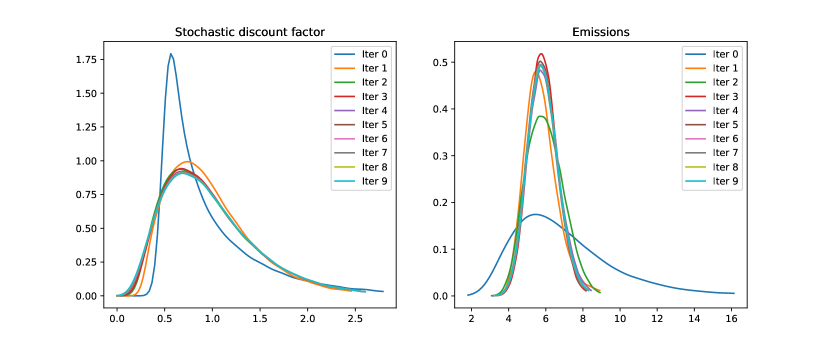
Figure 1: Convergence of the distribution of stochastic discount factor $\xi$ (left graph) and of the total average emissions.

Impact of climate risk on the decarbonization dynamics

In the first series of tests, we assume that there are no green investors ($\lambda=0$) and study the impact of climate risk on the decarbonization dynamics by changing the parameter $\gamma$ (volatility of the emission penalty). Figure 2 shows the distribution of total average emissions (left graph) and expected emissions of the representative company (with carbon intensity of production equal to 1) per unit of time (right graph), for different values of the volatility of emission penalty $\gamma$. We see that as the intensity of climate risk/uncertainty grows, every company and the entire market increase their carbon emissions. This phenomenon has already been observed in De Angelis et al. (2022): lax or uncertain climate policies do not encourage companies to reduce their emissions.

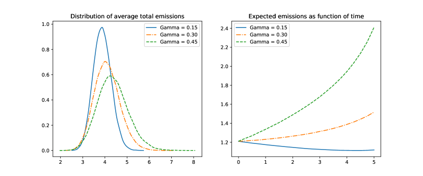
Figure 2: Distribution of total average emissions (left) and expected emissions of the representative company per unit of time (right), for different values of the volatility of emission penalty $\gamma$.

Impact of green investors on the decarbonization dynamics

We now illustrate the impact of the proportion and the environmental concern of the green investors on the total average emissions of all companies. Figure 3 shows the distribution of total average emissions (left graph) and expected emissions of the representative company per unit of time (right graph), for different values of the environmental concern of green investors $\lambda$, with $\gamma=0.3$ and $\rho=0.5$. We see that as the environmental concern grows, the distribution of total average emissions shifts to the left and narrows down, while the expected emissions decrease for all dates. Figure 4 illustrates the impact of the proportion of green investors $\rho$, for $\gamma=0.3$ and $\lambda=0.4$, and we see that increasing the proportion of green investors leads to a considerable reduction of carbon emissions.

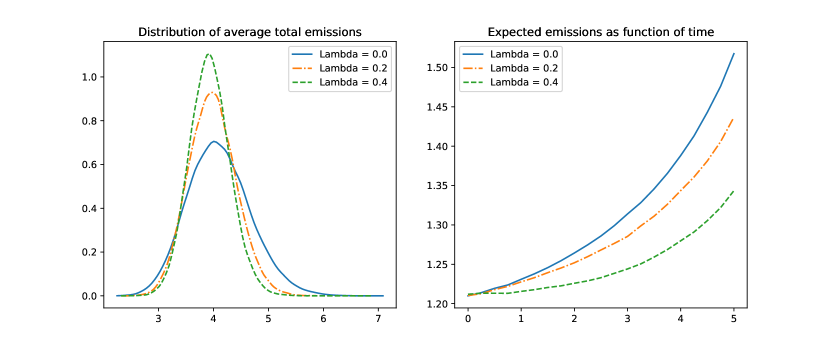
Figure 3: Distribution of total average emissions (left) and expected emissions of the representative company per unit of time (right), for different values of the environmental concern of green investors $\lambda$.

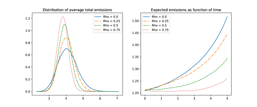
Figure 4: Distribution of total average emissions (left) and expected emissions of the representative company per unit of time (right), for different values of the proportion of green investors $\rho$.

Impact of the green investors on share prices

We now discuss the impact of the climate risk, the fraction and the environmental concern of green investors on the share price of the representative company. Table 1 shows the impact of various parameters on the two components of the price formula (29): $P_{1}$ is the coefficient multiplied by the firm value $V$, and $P_{2}$ is the coefficient multiplied by the squared emission efficacy $C_{0}^{2}$. We see that the first component (sensitivity to firm value) is quite stable. Indeed, the quantity $\mathbb{E}[\xi_{T}\overline{\mathcal{E}}_{T}]$ only weakly depends on $\xi$, because $\mathbb{E}[\xi]=1$ and the volatility $\sigma_{0}$ is not very high in our examples. On the other hand, the sensitivity to emission efficacy $P_{2}$ changes considerably between different tests. First, this sensitivity is always positive: all things being equal, carbon-efficient companies will enjoy higher stock prices than carbon-intensive companies. Second, this sensitivity increases when there is more climate risk / uncertainty (i.e., when $\gamma$ is high). This happens because, when climate uncertainty increases, all companies will emit more carbon, create more value and therefore pay higher dividends. However, carbon efficient companies create more value with one unit of extra emissions than carbon intensive companies, and are less exposed to climate risk, so that the spread between green and brown company share prices will grow. Finally, the sensitivity of share price to emission efficacy appears to decrease when the proportion of green investors and their environmental stringency grow. Indeed, in a market with many green-minded investors, all companies will emit less carbon, pay lower dividends and thus have lower share prices.

$\gamma$	$\lambda$	$\rho$	$P_{1}$	$P_{2}$
Impact of $\gamma$
$0.15$	$0$	$0.5$	$1.2102\pm 0.0004$	$6.260\pm 0.011$
$0.3$	$0$	$0.5$	$1.2112\pm 0.0003$	$6.928\pm 0.014$
$0.45$	$0$	$0.5$	$1.2128\pm 0.0003$	$8.143\pm 0.010$
Impact of $\lambda$
$0.3$	$0$	$0.5$	$1.2112\pm 0.0003$	$6.928\pm 0.014$
$0.3$	$0.2$	$0.5$	$1.2103\pm 0.0003$	$6.834\pm 0.017$
$0.3$	$0.4$	$0.5$	$1.2115\pm 0.0003$	$6.730\pm 0.019$
Impact of $\rho$
$0.3$	$0.4$	$0.0$	$1.2112\pm 0.0003$	$6.928\pm 0.014$
$0.3$	$0.4$	$0.25$	$1.2108\pm 0.0005$	$6.825\pm 0.020$
$0.3$	$0.4$	$0.5$	$1.2115\pm 0.0003$	$6.730\pm 0.019$
$0.3$	$0.4$	$0.75$	$1.2119\pm 0.0004$	$6.710\pm 0.020$
$0.3$	$0.4$	$1.0$	$1.2113\pm 0.0003$	$6.595\pm 0.021$

Table 1: Two components of the price formula (29): $P_{1}$ is the sensitivity to the firm value $V$, and $P_{2}$ is the sensitivity to the squared emission efficacy $C_{0}^{2}$. The standard errors quantify the Monte Carlo error only and were computed by running the test 10 times.

7 Conclusion

In this paper we develop a model for the decarbonization of a large financial market, arising from an equilibrium dynamics involving companies and investors, and built using the analytical framework of mean-field games. In our model, emission schedules are stochastic and may change dynamically depending on the firm’s own information, the materialization of climate risk and other market-wide or economy-wide factors. The model allows us to study the impact of climate risk and of the environmental concern of green investors on the market decarbonization dynamics in a stochastic framework: we can, for example, compute the distribution of aggregate emissions depending on the realization of common risk factors. Here, we suppose that there are two representative investors (regular and green) who have access to the same information set. In future research, the model could be extended to include many investors with varying degree of greenness and with access to information. Equilibrium dynamics will then need to be determined both at the level of companies and at the level of investors, leading to a two-stage mean-field game. Another promising direction would be to quantify the speed of convergence of the $n$-firm model to the mean-field setting, to understand how well the mean-field model approximates smaller markets.

References

• Achdou et al. (2022) Achdou, Y., J. Han, J.-M. Lasry, P.-L. Lions, and B. Moll (2022). Income and wealth distribution in macroeconomics: A continuous-time approach. The Review of Economic Studies 89(1), 45–86.
• Alekseev et al. (2022) Alekseev, G., S. Giglio, Q. Maingi, J. Selgrad, and J. Stroebel (2022). A quantity-based approach to constructing climate risk hedge portfolios. Technical report, National Bureau of Economic Research.
• Anderson and Raimondo (2008) Anderson, R. M. and R. C. Raimondo (2008). Equilibrium in continuous-time financial markets: Endogenously dynamically complete markets. Econometrica 76(4), 841–907.
• Andersson et al. (2016) Andersson, M., P. Bolton, and F. Samama (2016). Hedging climate risk. Financial Analysts Journal 72(3), 13–32.
• Ang and Chen (2007) Ang, A. and J. Chen (2007). CAPM over the long run: 1926–2001. Journal of Empirical Finance 14(1), 1–40.
• Avramov et al. (2022) Avramov, D., S. Cheng, A. Lioui, and A. Tarelli (2022). Sustainable investing with ESG rating uncertainty. Journal of Financial Economics 145(2), 642–664.
• Barrasso and Touzi (2022) Barrasso, A. and N. Touzi (2022). Controlled diffusion mean field games with common noise and McKean–Vlasov second order backward SDEs. Theory of Probability & Its Applications 66(4), 613–639.
• Berk and van Binsbergen (2021) Berk, J. and J. H. van Binsbergen (2021). The impact of impact investing. Available at SSRN 3909166.
• Bolton and Kacperczyk (2021) Bolton, P. and M. Kacperczyk (2021). Do investors care about carbon risk? Journal of financial economics 142(2), 517–549.
• Bourgey et al. (2022) Bourgey, F., E. Gobet, and Y. Jiao (2022). Bridging socioeconomic pathways of CO2 emission and credit risk. Annals of Operations Research, 1–22.
• Bredies et al. (2009) Bredies, K., D. A. Lorenz, and P. Maass (2009). A generalized conditional gradient method and its connection to an iterative shrinkage method. Computational Optimization and Applications 42(2), 173–193.
• Brezis (2010) Brezis, H. (2010). Functional Analysis, Sobolev Spaces and Partial Differential Equations. Universitext. Springer New York.
• Cardaliaguet et al. (2019) Cardaliaguet, P., F. Delarue, J.-M. Lasry, and P.-L. Lions (2019). The master equation and the convergence problem in mean field games. Princeton University Press.
• Carmona and Delarue (2018a) Carmona, R. and F. Delarue (2018a). Probabilistic theory of mean field games with applications, Volume 2. Springer.
• Carmona and Delarue (2018b) Carmona, R. and F. Delarue (2018b). Probabilistic Theory of Mean Field Games with Applications II: Mean Field Games with Common Noise and Master Equations, Volume 84. Springer.
• Carmona et al. (2016) Carmona, R., F. Delarue, and D. Lacker (2016). Mean field games with common noise. The Annals of Probability 44(6), 3740–3803.
• Casgrain and Jaimungal (2020) Casgrain, P. and S. Jaimungal (2020). Mean-field games with differing beliefs for algorithmic trading. Mathematical Finance 30(3), 995–1034.
• Chowdhry et al. (2019) Chowdhry, B., S. W. Davies, and B. Waters (2019). Investing for impact. The Review of Financial Studies 32(3), 864–904.
• De Angelis et al. (2022) De Angelis, T., P. Tankov, and O. D. Zerbib (2022). Climate impact investing. Management Science (published online).
• de la Vallée Poussin (1915) de la Vallée Poussin, C.-J. (1915). Sur l’intégrale de Lebesgue. Transactions of the American Mathematical Society, 435–501.
• Duffie (1986) Duffie, D. (1986). Stochastic equilibria: Existence, spanning number, and the ’no expected financial gain from trade’ hypothesis. Econometrica 54, 1161–1183.
• Duffie and Huang (1985) Duffie, D. and C.-F. Huang (1985). Implementing Arrow-Debreu equilibria by continuous trading of few long-lived securities. Econometrica 53, 1337–1356.
• Dunford and Schwartz (1988) Dunford, N. and J. T. Schwartz (1988). Linear operators, part 1: general theory, Volume 10. John Wiley & Sons.
• Engle et al. (2020) Engle, R. F., S. Giglio, B. Kelly, H. Lee, and J. Stroebel (2020). Hedging climate change news. The Review of Financial Studies 33(3), 1184–1216.
• Féron et al. (2022) Féron, O., P. Tankov, and L. Tinsi (2022). Price formation and optimal trading in intraday electricity markets. Mathematics and Financial Economics 16(2), 205–237.
• Frank and Wolfe (1956) Frank, M. and P. Wolfe (1956). An algorithm for quadratic programming. Naval research logistics quarterly 3(1-2), 95–110.
• Fu et al. (2021) Fu, G., P. Graewe, U. Horst, and A. Popier (2021). A mean field game of optimal portfolio liquidation. Mathematics of Operations Research 46(4), 1250–1281.
• Fujii and Takahashi (2022) Fujii, M. and A. Takahashi (2022). A mean field game approach to equilibrium pricing with market clearing condition. SIAM Journal on Control and Optimization 60(1), 259–279.
• Gomes et al. (2021) Gomes, D. A. et al. (2021). A mean-field game approach to price formation. Dynamic Games and Applications 11(1), 29–53.
• Green and Roth (2021) Green, D. and B. Roth (2021). The allocation of socially responsible capital. Available at SSRN 3737772.
• Heinkel et al. (2001) Heinkel, R., A. Kraus, and J. Zechner (2001). The effect of green investment on corporate behavior. Journal of financial and quantitative analysis 36(4), 431–449.
• Huang (1987) Huang, C.-F. (1987). An intertemporal general equilibrium asset pricing model: The case of diffusion information. Econometrica: Journal of the Econometric Society 55, 117–142.
• Huang et al. (2018) Huang, H. H., J. Kerstein, and C. Wang (2018). The impact of climate risk on firm performance and financing choices: An international comparison. Journal of International Business Studies 49(5), 633–656.
• Huang et al. (2006) Huang, M., R. P. Malhamé, and P. E. Caines (2006). Large population stochastic dynamic games: closed-loop McKean-Vlasov systems and the Nash certainty equivalence principle. Communications in Information & Systems 6(3), 221–252.
• Hugonnier et al. (2012) Hugonnier, J., S. Malamud, and E. Trubowitz (2012). Endogenous completeness of diffusion driven equilibrium markets. Econometrica 80(3), 1249–1270.
• Ilhan et al. (2021) Ilhan, E., Z. Sautner, and G. Vilkov (2021). Carbon tail risk. The Review of Financial Studies 34(3), 1540–1571.
• Jagannathan et al. (1995) Jagannathan, R., E. R. McGrattan, et al. (1995). The CAPM debate. Federal Reserve Bank of Minneapolis Quarterly Review 19(4), 2–17.
• Krueger et al. (2020) Krueger, P., Z. Sautner, and L. T. Starks (2020). The importance of climate risks for institutional investors. The Review of Financial Studies 33(3), 1067–1111.
• Lacker and Soret (2020) Lacker, D. and A. Soret (2020). Many-player games of optimal consumption and investment under relative performance criteria. Mathematics and Financial Economics 14(2), 263–281.
• Landier and Lovo (2020) Landier, A. and S. Lovo (2020). ESG investing: How to optimize impact? HEC Paris Research Paper No. FIN-2020-1363.
• Lasry and Lions (2007) Lasry, J.-M. and P.-L. Lions (2007). Mean field games. Japanese journal of mathematics 2(1), 229–260.
• Luttmer (2007) Luttmer, E. G. J. (2007). Selection, growth, and the size distribution of firms. The Quarterly Journal of Economics 122(3), 1103–1144.
• Morningstar Manager Research (2022) Morningstar Manager Research (2022). Investing in times of climate change. Technical report, Morningstar.
• Oehmke and Opp (2022) Oehmke, M. and M. M. Opp (2022). A theory of socially responsible investment. Swedish House of Finance Research Paper (20-2).
• Pástor et al. (2021) Pástor, L., R. F. Stambaugh, and L. A. Taylor (2021). Sustainable investing in equilibrium. Journal of Financial Economics 142(2), 550–571.
• Protter (2005) Protter, P. E. (2005). Stochastic differential equations. In Stochastic integration and differential equations, pp. 249–361. Springer.
• Revuz and Yor (2013) Revuz, D. and M. Yor (2013). Continuous martingales and Brownian motion, Volume 293. Springer Science & Business Media.
• Riedel and Herzberg (2013) Riedel, F. and F. Herzberg (2013). Existence of financial equilibria in continuous time with potentially complete markets. Journal of Mathematical Economics 49(5), 398–404.