Quasinormal Modes in Noncommutative Schwarzschild Black Holes

Abstract

We investigate the quasinormal modes of a massless scalar field in a Schwarzschild black hole, which is deformed due to noncommutative corrections. We present the deformed Schwarzschild black hole solution, which depends on the noncommutative parameter $\Theta$, and we extract the master equation as a Schrödinger-like equation, giving the explicit expression of the effective potential which is modified due to the noncommutative corrections. We solve the master equation numerically and we find that the noncommutative gravitational corrections “break” the stability of the scalar perturbations in the long time evolution of the massless scalar field. The significance of these results is twofold. Firstly, our results can be related to the detection of gravitational waves by the near future gravitational wave detectors, such as LISA, which will have a significantly increased accuracy. In particular, these observed gravitational waves produced by binary strong gravitational systems have oscillating modes which can provide valuable information. Secondly, our results can serve as an additional tool to test the predictions of general relativity, as well as to examine the possible detection of this kind of gravitational corrections.

I Introduction

In a seminal paper by Snyder [1] , there appeared for the first time the idea that spacetime can be described in noncommutative (NC) frameworks. Such a consideration, and more generally the interest for the NC physics, received a renewed interest later on due to the discovery of the Seiberg-Witten map, which essentially relates the NC theories to the commutative gauge theories [2] . The latter has played a relevant role in the understanding of NC physics on a fundamental level, that is the spacetime symmetries and the unitary properties of these theories [3] ; [4] ; [5] ; [6] ; [6b] ; [7] ; [8] ; [9] , and the possible experimental signatures [10] ; [11] ; [11]b ; 20Ko ; 21Ko (see also [3] ; [4] ; [5] ; [6] ; [6b] ; [7] ; [8] ; [9]a ; [9] ; [10] ; [11] ; [11]b ; [12]a ; [12] for the violation of spacetime symmetries and [6] ; [6b] ; [13] ; [OMMY] for the full Lorentz invariance). Furthermore, in the framework of string theories, the low-energy limit yields in a natural way a quantized structure of spacetime 18Ko ; [2] ; 20Ko ; 21Ko , while at high-energy scales the noncommutativity of spacetime may lead to a deep insight on its quantum nature [2] ; [6] ; [6b] .

In the NC frameworks, one defines the fields over phase space in which the ordinary product of fields is replaced by the Moyal product. Due to the Seiberg-Witten map, this theory turns out to be equivalent to commutative gauge theories in which the fields are expanded in terms of a NC parameter 5Sa ; 5Sa1 ; 5Sa2 ; 5Sa3 ; 5Sa4 ; 5Sa5 ; 6Sa ; 22Ko ; 23Ko ; 24Ko ; 25Ko . In this respect, the formulation of gravity as a commutative equivalent gauge theory turns out to be very promising (for details, see 8Ch ; 10Ch ; 11Ch ; 12Ch ; 12Chb ; 13Ch ; 14Ch ; 15Ch ; 15Chb ; 16Ch ; 17Ch ; 18Ch ; 19Ch ; Manolakos:2019fle ; Manolakos:2022ihc ).

On the other hand, recently the study of the quasinormal modes (QNMs) Nollert:1999ji ; Konoplya:2011qq ; Isi:2021iql has generated a lot of interest in the scientific community Cai:2015fia ; Cardoso:2019mqo ; McManus:2019ulj ; Guo:2021enm ; Ejlli:2019bqj , since they allow for the investigation of gravity in the strong-field regime. This is certainly possible due to experiments with increasing accuracy, such as the Event Horizon Telescope (EHT), which has captured the first image of a black hole EventHorizonTelescope:2019dse ; EventHorizonTelescope:2019ggy ; EventHorizonTelescope:2020qrl , and the LIGO-Virgo collaboration which has detected the first gravitational wave signal LIGOScientific:2016aoc ; LIGOScientific:2016lio . These observations opened the possibility of studying black hole features near the event horizon, as well as of probing modified gravity theories Cai:2018rzd ; Yan:2019hxx ; Li:2021mzq ; Jusufi:2021fek , or quantum gravity corrections, which is the subject of this paper. More specifically, since QNMs represent characteristic modes of the perturbation equations in a given gravitational background Zerilli:1970se ; Chandrasekhar:1975zza ; Kokkotas:1999bd ; Berti:2009kk ; Hatsuda:2021gtn , they provide information on the geometry of spacetime. Such a feature highlights the important role of QNMs in connection with the physics of gravitational waves (GWs). In fact, on one hand GWs allow us to make observations in order to test general relativity (GR) Dreyer:2003bv ; Berti:2005ys ; Isi:2019aib , and on the other hand the predictions of QNMs properties allow us to constrain the gravitational theories beyond GR Cano:2021myl ; Wang:2004bv ; Blazquez-Salcedo:2016enn ; Franciolini:2018uyq ; Becar:2019hwk ; Aragon:2020xtm ; Liu:2020qia ; Karakasis:2021tqx ; Gonzalez:2022upu ; Ishibashi:2003ap ; Zhao:2022gxl ; Chowdhury:2022zqg .

The aim of this paper is to investigate the QNMs in the case of black hole solutions in NC gravity. In particular, we refer to the deformed Schwarzschild solution, where the corrections are induced by the NC parameter $\Theta$. For this metric, we compute the corresponding QNM frequency of a massless scalar field. The noncommutativity of gravity is induced by a NC coordinate product given by

$$[x^{\mu},x^{\nu}]=i\Theta^{\mu\nu},$$ (1)

where the (antisymmetric) tensor $\Theta^{\mu\nu}$ is a $c$-number (here the Greek indices are used for the spacetime coordinates $\mu,\nu=0,\ldots,3$) and accounts for the degree of quantum fuzziness of spacetime. At this point it should be noted that different approaches have been proposed in which the NC coordinates occur, for instance in the $q$-deformed theories [18] . The NC parameter $\Theta^{\mu\nu}$ has been constrained in several frameworks: in low-energy measurements 26Ko ; jabbari ; jabbarib ; dastheta , in Lorentz symmetry breaking 28Ko ; 29Ko , in cosmology and physics of the primordial Universe 30Ko ; 31Ko ; GaeCQG ; Addazi:2021xuf , and in gravitational physics 8Ch ; 33Ko ; 34Ko ; 35Ko ; 36Ko ; 37Ko ; 38Ko ; 39Ko ; KoGW16 ; KoBH09 ; GUPNC ; CANTATA:2021ktz . It is noteworthy that in the aforesaid models the NC corrections appear to second order in $\Theta$. In TABLE 1, we report some bounds on $\Theta^{\mu\nu}$.

Bounds on $\Theta$	Physical framework	Refs.
$\Theta<(1\text{TeV})^{-2}$	Nucleus wave function	Carroll ; 29Ko
$\Theta<10^{-8}$GeV-2	Lamb shift corrections	jabbari ; jabbarib
$\Theta<10^{-7}$GeV-2	CMB physics	dastheta
$|\Theta|<10^{-11}$GeV-1	Generalized uncertainty principle (GUP)	GUPNC
$|\Theta|<8.4\times 10^{-38}$GeV-2	GW signal detected by LIGO/Virgo collaboration	KoGW16

Table 1: Bounds on the NC parameter $\Theta$ (or $|\Theta|$) inferred in different experiments, where $\Theta$ refers to different components of $\Theta^{\mu\nu}$ (see the corresponding references). The different units of $\Theta$ in the GUP case arises from the fact that there the bounds have been inferred in spherical coordinates and therefore $[\Theta]=[\Theta^{r\theta}]=\text{GeV}^{-1}$, while in Cartesian coordinates $[\Theta]=\text{GeV}^{-2}$.

The rest of the paper is organized as follows. In Section II, we review the NC gravity and present the modified Schwarzschild black hole solutions which are $\Theta$-depending. In Section III, we derive the form of the Schrödinger-like equation. In Section IV, we numerically solve the Schrödinger-like equation, and get the time evolution of the dominant mode. In Section V, we present and discuss our conclusions.

II $\Theta^{\mu\nu}$- Schwarzschild black holes

In this Section we briefly review the NC black hole solutions following the analysis of Ref. 18Ch . The NC corrections to the Schwarzschild black hole geometry, which are a $\Theta$-expansion, are investigated (for other solutions of the deformed Einstein field equations the reader could see 17Ch ; 18Ch ; 22Ko ; 23Ko ; KoGW16 ; KoBH09 and references therein). The important point is that the Schwarzschild black hole solution is exact. One starts by writing the deformed metric in terms of the tetrad fields, namely

$${\hat{g}}_{\mu\nu}(x,\Theta)=\frac{1}{2}\left({\hat{e}}_{\mu}^{a}\ast{\hat{e}}_{\nu}^{b\,\dagger}+{\hat{e}}_{\mu}^{b}\ast{\hat{e}}_{\nu}^{a\,\dagger}\right)\eta_{ab},$$ (2)

where the “^†” denotes the complex conjugation, the Latin indices are used for the tangent space basis $a,b=0,\dots,3$, and the “$\ast$” stands for the Moyal product which is defined as $\phi(x)\ast\chi(x)\equiv e^{\frac{i}{2}\Theta^{\mu\nu}\partial_{x^{\mu}}\partial_{y^{\nu}}}\phi(x)\chi(y)\Big{|}_{y\to x}$. The tetrads, as gauge fields, are expanded in terms of the $\Theta^{\nu\rho}$-parameter as

$${\hat{e}}^{a}_{\mu}(x,\Theta)=e^{a}_{\mu}(x)-i\Theta^{\nu\rho}e^{a}_{\mu\nu\rho}(x)+\Theta^{\nu\rho}\Theta^{\alpha\sigma}e^{a}_{\nu\rho\alpha\sigma}(x)+{\cal O}(\Theta^{3}),$$ (3)

with

$$e^{a}_{\mu\nu\rho}(x)=\frac{1}{4}[\omega^{ac}_{\nu}\partial_{\rho}e^{d}_{\mu}+(\partial_{\rho}\omega_{\mu}^{ac}+R_{\rho\mu}^{ac})e^{d}_{\nu}]\eta_{cd},$$

and similar expressions exist for the other terms of the expansion 18Ch . In the above equations, $R_{\rho\mu}^{ac}$ is the curvature tensor and $\omega_{\mu}^{ac}$ is the connection.

Following the quantization procedure of Refs. 11a ; 12a ; 13a ; 14a for the Schwarzschild black hole metric, one needs to fix the Moyal algebra. In terms of the spherical coordinates $x^{\mu}=(t,r,\theta,\phi)$, the algebra is deformed as

$$\Theta^{\mu\nu}=\Theta\begin{pmatrix}0&0&1&0\\ 0&0&0&0\\ -1&0&0&0\\ 0&0&0&0\end{pmatrix},$$ (4)

where $\Theta$ is the deformation parameter, which as discussed in the Introduction, gives rise to the simplest model of a NC spacetime. The non-deformed Schwarzschild black hole geometry is described by the line element $ds^{2}=g_{\mu\nu}^{(S)}dx^{\mu}dx^{\nu}$, with

$$g_{\mu\nu}^{(S)}=\text{diag}(-{\cal F}(r),{\cal F}^{-1}(r),r^{2},r^{2}\sin^{2}\theta)\,,\quad{\cal F}(r)\equiv 1-\frac{\alpha}{r}\,,\quad\alpha\equiv 2GM,$$ (5)

where $M$ is the mass of the gravitational source. Hence, the corresponding vierbein fields are

$$e_{\mu}^{0}=({\cal F},0,0,0),\quad e_{\mu}^{1}=(0,{\cal F}^{-1},0,0)\,,\quad e_{\mu}^{2}=(0,0,r,0)\,,\quad e_{\mu}^{3}=(0,0,0,r\sin\theta)~{}.$$ (6)

Furthermore, the components of the $\Theta$-Schwarzschild black hole metric, according to (2), are given by

$${\hat{g}}_{\mu\nu}=g_{\mu\nu}^{(S)}+h_{\mu\nu}^{(NC)}$$ (7)

with

$$h_{00}^{(NC)} = -\frac{\alpha(8r-11\alpha)}{16r^{4}}\Theta^{2}+{\cal O}(\Theta^{4})\,,$$ (8)

$$h_{rr}^{(NC)} = -\frac{\alpha(4r-3\alpha)}{16r^{2}(r-\alpha)^{2}}\Theta^{2}+{\cal O}(\Theta^{4})\,,$$ (9)

$$h_{\theta\theta}^{(NC)} = \frac{2r^{2}-17\alpha(r-\alpha)}{32r(r-\alpha)}\Theta^{2}+{\cal O}(\Theta^{4})\,,$$ (10)

$$h_{\phi\phi}^{(NC)} = \frac{(r^{2}+\alpha r-\alpha^{2})\cos^{2}\theta-\alpha(2r-\alpha)}{16r(r-\alpha)}\Theta^{2}+{\cal O}(\Theta^{4}),$$ (11)

where $h_{\mu\nu}^{(NC)}$ quantifies the NC corrections to the Schwarzschild black hole metric. The embedding of the $2$-dimensional slides of constant $r$ and $t$ described by this metric is shown in FIG. 1.

At this point, a number of comments are in order. First, the standard Schwarzschild black hole solution is recovered in the limit $\Theta\to 0$, as anticipated. Second, as mentioned in the Introduction, the corrections enter in the metric as $\Theta^{2}$, that is they are of second order in the deformation parameter $\Theta$ (this is a general aspect of NC gravity 8Ch ; 33Ko ; 34Ko ; 35Ko ; 36Ko ; 37Ko ; 38Ko ; 39Ko ; KoGW16 ; KoBH09 ). Third, it is worth of note that since we are using spherical coordinates, the dimension of $\Theta$ are $[\Theta]^{2}=[L]^{2}=[M]^{-2}$ 18Ch ; 14a ; 12a ; setare ; singh ; alavi , contrary to the standard canonical quantization, which is in Cartesian coordinates, where the NC parameter $\Theta^{2}$ has dimensions $[L]^{4}$).

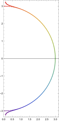
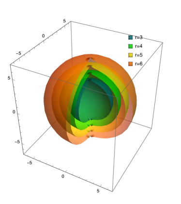
Figure 1: The left panel shows the embedded shape $(\rho(\theta),z(\theta))$ for a constant $\varphi$ and $r=3$. The thick curve depicts the case of the NC metric, while, given for comparison, the dashed curve corresponds to the sphere geometry. The color of the curve indicates the $\theta$ value. The right panel shows the $3$-dimensional shape of the constant $r$ slides. The color of the surface indicates the value of $r$. The parameter choice is $\Theta^{2}=0.2$ for both plots, and we have adopted $M=1$.

III Quasinormal Modes in Noncommutative black hole spacetime

Now we proceed to the investigation of the QNMs in the deformed, due to noncommutativity, Schwarzschild black holes. We start with the derivation of the effective potential by writing the Klein-Gordon field equation in a Schrödinger-like form. For this reason, we adopt the analysis of Ref.ChenTsao where a general formalism has been developed.

The deformed Schwarzschild black hole metric is parameterized as

$$g_{tt} = -\left(1-\frac{2M}{r}\right)\left(1+\epsilon A_{j}(r)\cos^{j}{\theta}\right)\,,$$ (12)

$$g_{rr} = \left(1-\frac{2M}{r}\right)^{-1}\left(1+\epsilon B_{j}(r)\cos^{j}{\theta}\right)\,,$$ (13)

$$g_{\theta\theta} = r^{2}\left(1+\epsilon C_{j}(r)\cos^{j}{\theta}\right)\,,$$ (14)

$$g_{\varphi\varphi} = r^{2}\sin^{2}\theta\left(1+\epsilon D_{j}(r)\cos^{j}{\theta}\right)\,,$$ (15)

$$g_{tr} = \epsilon a_{j}(r)\cos^{j}{\theta}\,,\qquad g_{t\theta}=\epsilon b_{j}(r)\cos^{j}{\theta}\,,$$ (16)

$$g_{r\theta} = \epsilon c_{j}(r)\cos^{j}{\theta}\,,\qquad g_{r\varphi}=\epsilon d_{j}(r)\cos^{j}{\theta}\,,$$ (17)

$$g_{\theta\varphi} = \epsilon e_{j}(r)\cos^{j}{\theta},$$ (18)

where the index $j$ stands for summations running upward from $j=0$. By comparing (13)-(18) with (8)-(11), one obtains

$$\epsilon = \Theta^{2}\,,$$ (19)

$$A_{0}(r) = \frac{\alpha(8r-11\alpha)}{16r^{3}(r-\alpha)}\,,$$ (20)

$$B_{0}(r) = -\frac{\alpha(4r-3\alpha)}{16r^{3}(r-\alpha)}\,,$$ (21)

$$C_{0}(r) = \frac{2r^{2}-17\alpha(r-\alpha)}{32r^{3}(r-\alpha)}\,,$$ (22)

$$D_{0}(r) = \frac{(r^{2}+\alpha r-\alpha^{2})\cos^{2}\theta-\alpha(2r-\alpha)}{16r^{3}(r-\alpha)\sin^{2}\theta}=-\frac{\alpha(2r-\alpha)}{16r^{3}(r-\alpha)}\,,$$ (23)

$$D_{j}(r) = \frac{1+(-1)^{j}}{32r^{2}}\quad\quad(\text{for}\;j>0)\;,$$ (24)

$$a_{j}(r) = b_{j}(r)=c_{j}(r)=d_{j}(r)=e_{j}(r)=0~{}.$$ (25)

Next, we consider massless scalar waves propagating in the deformed Schwarzschild black hole spacetime, with equation of motion of the form

$$\Box\psi=0~{}.$$ (26)

Exploiting the fact that there are two Killing vectors, i.e., $\partial_{t}$ and $\partial_{\varphi}$, this equation can be decomposed through

$$\Box\psi=\int_{-\infty}^{\infty}d\omega\sum_{m=-\infty}^{\infty}e^{i(m\varphi-\omega t)}\mathcal{D}_{m,\omega}^{2}\psi_{m,\omega}(r,\theta),$$ (27)

where the Fourier modes of the wave function, i.e., $\psi_{m,\omega}$, satisfy the equation

$$\mathcal{D}_{m,\omega}^{2}\psi_{m,\omega}=0,$$ (28)

with $m$ the azimuthal number and $\omega$ the mode frequency. The operator $\mathcal{D}_{m,\omega}^{2}$ can be written (up to first order in $\epsilon$) as

$$\mathcal{D}_{m,\omega}^{2}=\mathcal{D}_{(0)m,\omega}^{2}+\epsilon\mathcal{D}_{(1)m,\omega}^{2}~{}.$$ (29)

The zeroth order operator, i.e., $\mathcal{D}_{(0)m,\omega}^{2}$, is given by

$$\mathcal{D}^{2}_{(0)m,\omega}=-\left[\omega^{2}-\frac{m^{2}{\cal F}(r)}{r^{2}\sin^{2}{\theta}}\right]-\frac{{\cal F}(r)}{r^{2}}\partial_{r}\left[r^{2}{\cal F}(r)\partial_{r}\right]-\frac{{\cal F}(r)}{r^{2}\sin{\theta}}\partial_{\theta}\left(\sin{\theta}\partial_{\theta}\right),$$ (30)

while the first order operator, i.e., $\mathcal{D}_{(1)m,\omega}^{2}$, is presented in (49) of Appendix A ChenTsao . In addition, the Fourier modes of the wavefunction, i.e., $\psi_{m,\omega}$, can be expanded as

$$\psi_{m,\omega}=\sum_{l^{\prime}=|m|}^{\infty}P_{l^{\prime}}^{m}(x)R_{l^{\prime},m}(r),$$ (31)

where $x=\cos\theta$ and the Legendre functions $P_{l}^{m}(x)$ are the angular basis of (30).

Our aim now is to extract the master equation in a Schrödinger-like form, where the latter includes the effective potential. First, we introduce the tortoise radius $r_{*}$ ChenTsao

$$\frac{dr}{dr_{*}}={\cal F}(r)\left[1+\frac{\epsilon}{2}b^{j}_{lm}\left(A_{j}-B_{j}\right)\right],$$ (32)

and a new radial wave function $\Psi_{l,m}$

$$R_{l,m}=\frac{\Psi_{l,m}}{r}\left[1+\frac{\epsilon}{4}b^{j}_{lm}\left(A_{j}-B_{j}\right)-\epsilon\int dr\frac{Z_{lm}(r)}{4r^{2}}\right],$$ (33)

where

$$Z_{lm}(r)\equiv b^{j}_{lm}r^{2}\left(A_{j}^{\prime}-B_{j}^{\prime}+C_{j}^{\prime}+D_{j}^{\prime}\right)+4ig^{j}_{lm}d_{j}+\frac{4i\omega r^{2}b^{j}_{lm}a_{j}}{\cal F}~{}.$$

By substituting (32) and (33) into (26), we obtain the master equation written in a Schrödinger-like form

$$\partial_{r_{*}}^{2}\Psi_{l,m}+\omega^{2}\Psi_{l,m}=V_{\textrm{eff}}(r)\Psi_{l,m}$$ (34)

with the effective potential, i.e., $V_{\textrm{eff}}(r)$, to be of the form ChenTsao

$$V_{\textrm{eff}}(r) = l(l+1)\frac{{\cal F}}{r^{2}}+\frac{{\cal F}}{r}\frac{d{\cal F}}{dr}\left[1+\epsilon b^{j}_{lm}\left(A_{j}-B_{j}\right)\right]+\epsilon\Bigg{\{}\frac{{\cal F}}{r^{2}}\Big{[}a^{j}_{lm}\left(A_{j}-D_{j}\right)-c^{j}_{lm}\left(A_{j}-C_{j}\right)-\frac{b^{j}_{lm}}{4}\frac{d^{2}}{dr_{*}^{2}}\left(A_{j}-B_{j}\right)$$ (35)

$$-\frac{d^{j}_{lm}}{2}\left(A_{j}+B_{j}-C_{j}+D_{j}\right)+\,e^{j}_{lm}\partial_{r}\left({\cal F}c_{j}\right)\Big{]}+\frac{1}{4r^{2}}\frac{d}{dr_{*}}\left[b^{j}_{lm}r^{2}\frac{d}{dr_{*}}\left(A_{j}-B_{j}+C_{j}+D_{j}\right)\right]\Bigg{\}},$$

and with the coefficients $a^{j}_{lm}$, $b^{j}_{lm}$, $c^{j}_{lm}$, $d^{j}_{lm}$, and $e^{j}_{lm}$ to be given in Appendix B. The eikonal QNMs and photon geodesics, which form the photon sphere around black holes, are related, since in the eikonal limit, i.e., $l\gg 1$ the effective potential exhibits a peak located at the photon sphere. Interestingly enough, the spacetime deformation induced by the $\Theta^{2}$-terms implies that the effective potential does depend on $m$ (and besides that on $l$ as in absence of deformations), affecting the behavior of high-frequency modes that could be different for different values of $m$.

IV Quasinormal Mode calculation in characteristic integration method

In this section, we solve the Schrödinger-like equation (34) with the effective potential (35) utilizing the characteristic integration method. Therefore, we derive the time evolution of dominant QNM. In the following numerical calculation and plots, we choose $G=c=1$ and $M=1$.

IV.1 Adding up the terms for the effective potential

We can separate the effective potential into three parts: (i) the Schwarzschild effective potential, i.e., $V_{\mathrm{sch}}$, (ii) the contribution from the $j=0$ part, i.e., $V_{0}$, and (iii) the contribution from the $j>0$ part, i.e., $V_{j}$, and thus it reads

$$V_{\mathrm{eff}}(r)=V_{\mathrm{sch}}+V_{0}+V_{j},$$ (36)

where

$$V_{\mathrm{sch}}= l(l+1)\frac{{\cal F}}{r^{2}}+\frac{{\cal F}}{r}\frac{d{\cal F}}{dr},$$ (37)

$$V_{0}= \epsilon\frac{{\cal F}}{r}\frac{d{\cal F}}{dr}b^{0}_{lm}(A_{0}-B_{0})+\epsilon\left\{\frac{{\cal F}}{r^{2}}\left[a_{lm}^{0}\left(A_{0}-D_{0}\right)-c_{lm}^{0}\left(A_{0}-C_{0}\right)-\frac{d_{lm}^{0}}{2}\left(A_{0}+B_{0}-C_{0}+D_{0}\right)\right]\right.$$

$$\left.+\frac{1}{4r^{2}}\frac{d}{dr_{*}}\left[b_{lm}^{0}r^{2}\frac{d}{dr_{*}}\left(A_{0}-B_{0}+C_{0}+D_{0}\right)\right]-\frac{b_{lm}^{0}}{4}\frac{d^{2}}{dr_{*}^{2}}\left(A_{0}-B_{0}\right)\right\},$$ (38)

$$V_{j}= -\epsilon\frac{{\cal F}}{r^{2}}\sum_{j=1}^{\infty}\left(a^{j}_{lm}+\frac{1}{2}d^{j}_{lm}\right)D_{j}+\epsilon\sum_{j=1}^{\infty}\frac{1}{4r^{2}}\frac{d}{dr^{*}}\left(b^{j}_{lm}r^{2}\frac{d}{dr^{*}}\right)D_{j}~{}.$$ (39)

The calculation of the Schwarzschild contribution $V_{\mathrm{sch}}$ and the $j=0$ contribution $V_{0}$ is straightforward. Thus, we need to add up the terms of the $j>0$ part. Calculating the coefficients $a^{j}_{lm}$, $b^{j}_{lm}$, $c^{j}_{lm}$, $d^{j}_{lm}$ with the help of MATHEMATICA, we obtain for the case of $l=m=1$

$$a_{lm}^{j}=\frac{3(1+(-1)^{j})}{4(1+j)},\;b_{lm}^{j}=\frac{3[1+(-1)^{j}]}{2(1+j)(3+j)},\;c_{lm}^{j}=\frac{3[1+(-1)^{j}](-1+j)}{4(1+j)(3+j)},\;d_{lm}^{j}=\frac{3[1+(-1)^{j}]j}{2(1+j)(3+j)}~{}.$$ (40)

Now, we can add up the terms of the $j>0$ part of the effective potential and acquire

$$\sum_{j=1}^{\infty}\left(a^{j}_{lm}+\frac{1}{2}d^{j}_{lm}\right)D_{j}=\frac{3}{64r^{2}}$$ (41)

$$\sum_{j=1}^{\infty}\frac{1}{4r^{2}}\frac{d}{dr^{*}}\left(b^{j}_{lm}r^{2}\frac{d}{dr^{*}}\right)D_{j}$$

$$=\sum_{j=1}^{\infty}\frac{0.0234375\left(r^{4}-2r^{3}+0.075r-0.175\right)\left(r^{5}-6r^{4}+8r^{3}+0.3r^{2}-1.475r+1.75\right)\left(1+(-1)^{j}\right)^{2}}{(j+1)(j+3)(r-2)r^{12}}$$

$$=\frac{0.015625\left(r^{9}-8r^{8}+20r^{7}-14.125r^{6}-13.5r^{5}+31.75r^{4}-23.9375r^{3}-4.07812r^{2}+9.73437r-7.65625\right)}{r^{12}(r-2)}~{}.$$ (42)

Therefore, we obtain

$$V_{j}=\frac{1}{(r-2)^{3}r^{12}}(-0.003125r^{11}+0.01875r^{10}-0.025r^{9}-0.0494141r^{8}+0.143438r^{7}-0.0708594r^{6}$$

$$-0.0641836r^{5}+0.069917r^{4}-0.0288564r^{3}-0.00393164r^{2}+0.00434766r-0.00191406)~{}.$$ (43)

It is evident that now we are able to compute the explicit expression of the effective potential, i.e., (36), and, thus, we can plot its shape. In order to see how the effective potential of the deformed Schwarzschild black hole deviates from the effective potential of the standard Schwarzschild black hole solution, we plot both effective potentials in FIG. 2. It is easily seen that the difference between the two effective potentials is small. This means that the contribution from the $j=0$ part, i.e., $V_{0}$, and the contribution from the $j>0$ part, i.e., $V_{j}$, are small compared to the effective potential of the standard Schwarzschild black hole solution, i.e., $V_{\mathrm{sch}}$. This is also depicted in FIG. 3 in which we plot the contribution of the $j=0$ part and the contribution of the $j>0$ part to the modified effective potential. These graphs are plotted with parameter $\Theta^{2}=0.5$. The left panel is ploted with $l=m=1$, while the right panel is plotted with $l=3$, $m=1$. As we can see, both $j=0$ and $j>0$ contributions are quite small, and actually the $j>0$ contribution is even smaller than the $j=0$ contribution. However, for $m=1$, as $l$ gets larger, the contribution from the $j>0$ part also gets larger, and for $l=3$ this part is not negligible compared with the contribution of the $j=0$ part.

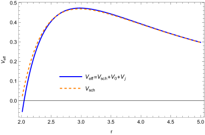
Figure 2: The effective potential $V_{\mathrm{eff}}(r)$ as a function of $r$, for $l=m=1$, and $\Theta^{2}=0.5$ for NC gravity.

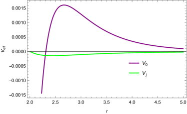
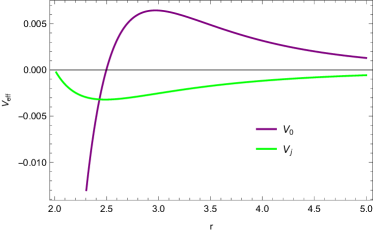
Figure 3: The contribution of the $j=0$ part, i.e. $V_{0}$, as well as the contribution of the $j>0$ part, i.e. $V_{j}$, to the effective potential $V_{\mathrm{eff}}(r)$, for $\Theta^{2}=0.5$. The left panel is for $l=m=1$, while the right panel is for $l=3$, $m=1$.

At this point it should be pointed out that the calculation of the explicit expression of the effective potential meets some divergence when $m=0$. In particular, for the summation that appears in the contribution of the $j>0$ part, we have an infinite summation up to $j=+\infty$. For the case of $m=0$, this summation is divergent, and, thus, we cannot get the explicit expression of the effective potential. For instance, for the case of $l=1$ and $m=0$, combining (39) and (40), we obtain

$$\sum_{j=0}^{\infty}\left(a^{j}_{lm}+\frac{1}{2}d^{j}_{lm}\right)D_{j}=\sum_{j=0}^{\infty}\frac{3(1+(-1)^{j})^{2}j}{64(1+j)(3+j)r^{2}}\sim\frac{3}{64r^{2}}\sum_{j=1}^{\infty}\frac{1}{j}~{}.$$ (44)

It is obvious that this infinite summation gives a divergent result. The same result is also obtained for the case of $l=0$ and $m=0$ as well as for the case $l=2$ and $m=0$. The conclusion is that we cannot carry out the computation for any value of $l$ when $m=0$.

At this point, one may think of adopting the analysis of Ref. ChenTsao and, thus, utilize (5.17) in ChenTsao which is an approximated expression of the effective potential for the case of $m=0$. A couple of comments are in order here. First, this result does not hold in our case since we do not have the eikonal limit, i.e., $l\gg 1$. Second, if we substitute $A_{2k}=A$ and $C_{2k}=C$ in this expression, then we will find that the summation in this case is also divergent.

Finally, in our case here the divergence is generic in the sense that the explicit expression of the effective potential is divergent due to the specific background geometry, namely the deformed Schwarzschild black hole spacetime. It is known that the case $m=0$ corresponds to the polar orbits which are the orbits of the photons that pass above or nearly above the poles. However, it is easily seen in FIG. 1, that the spacetime is not smooth at the poles due to the specific NC corrections. Therefore, polar orbits, and thus the case of $m=0$, should be excluded from the calculation of the explicit expression of the effective potential.

IV.2 The numerical function for the tortoise coordinate

The next step is to get the numerical function for the tortoise coordinate. Since we already have the function for $\frac{dr}{dr^{*}}$, i.e., (32), we can solve the corresponding differential equation to get $r^{*}(r)$, and then inverse this function to get $r(r^{*})$. The shape of these two functions with parameter choice $l=m=1$ and $\Theta^{2}=0.1$ is shown in FIG. 4.

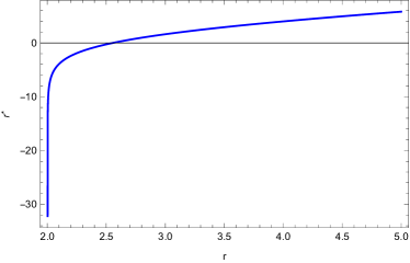
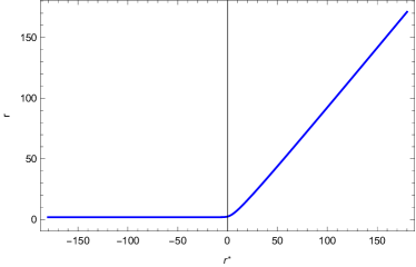
Figure 4: $r^{*}(r)$ as a function of $r$ (left panel), and $r(r^{*})$ as function of $r^{*}$ (right panel), for $l=m=1$ and $\Theta^{2}=0.1$.

However, we need to mention here that the function $r^{*}(r)$ works differently from the standard Schwarzschild black hole case. In the standard Schwarzschild black hole case, this function maps the spatial infinity to $r^{*}=+\infty$ and maps the event horizon $r=2M$ to $r^{*}=-\infty$. Here, $r^{*}=+\infty$ still stands for spatial infinity, but the position $r^{*}=-\infty$ does not correspond to the root of the metric function (see FIG. 5).

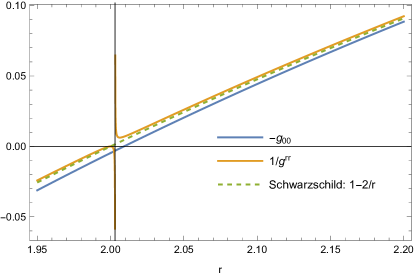
Figure 5: The metric functions form for $\Theta^{2}=0.1$. The vertical line stands for the value of $r$ corresponding to $r^{*}=-\infty$.

For convenience, we use $r_{r}$ to stand for this asymptotic value, namely, $r^{*}(r=r_{r})=-\infty$. It is known that the position of event horizon is defined through the relationship $g_{00}=g^{rr}=0$ and, thus, it is easily seen that $r_{r}$ does not correspond to the position of an horizon.

In FIG. 6, it is shown that the effective potential close to the position $r=r_{r}$ for the case of $l=m=1$ and $\Theta^{2}=0.1$. From this plot, it is obvious that the effective potential has a divergence at the position $r=2M$ and it takes negative values around $r=r_{r}$.

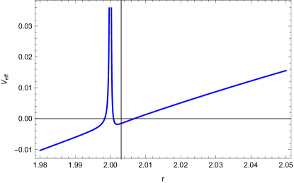
Figure 6: The shape of effective potential $V_{\text{eff}}\,(r)$ in (36), close to the horizon, for $l=m=1$ and $\Theta^{2}=0.1$. The vertical line marks the position $r=r_{r}$.

In FIG. 7, the effective potential $V_{\mathrm{eff}}$ is plotted as a function of the tortoise coordinate, namely $r^{*}$, for the case of $l=m=1$ and $\Theta^{2}=0.5$ for NC gravity. It can be easily seen that the shape of the effective potential of the deformed Schwarzschild black hole is nearly non-distinguishable from the effective potential of the standard Schwarzschild black hole solution. However, for the deformed Schwarzschild black hole case, the effective potential gets negative asymptotic values as $r^{*}$ goes to negative infinity. The aforesaid conclusions do not depend on the value of the parameter $\Theta^{2}$ as it is easily seen in FIG. 8 where we have plotted the effective potential $V_{\mathrm{eff}}$ for the case of $l=m=1$ and several values of $\Theta^{2}$.

As we will see later, this difference between the curves of the effective potential of the standard Schwarzschild black hole and the deformed ones causes the evolution of a massless test scalar field to be unstable.

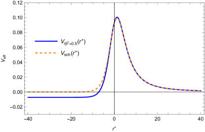
Figure 7: The shape of the effective potential in terms of the tortoise coordinate $r^{*}$, for $l=m=1$, and $\Theta^{2}=0.5$.

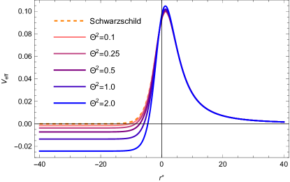
Figure 8: The shape of the effective potential in terms of the tortoise coordinate $r^{*}$, for $l=m=1$ and various values of $\Theta^{2}$.

IV.3 The time evolution of the dominant mode

In this section, we numerically solve the Schr$\ddot{\text{o}}$dinger-like equation utilizing the discretization method and then extract the time evolution of the dominant mode. For convenience, first we introduce the light-cone coordinates

$$u=t-r^{*},\;v=t+r^{*}~{}.$$ (45)

Then the Schr$\ddot{\text{o}}$dinger-like equation (34) can be written as

$$-4\frac{\partial^{2}\Psi_{l,m}(u,v)}{\partial u\partial v}-V_{\text{eff}}(u(r),v(r))\Psi_{l,m}(u,v)=0~{}.$$ (46)

Discretizing this equation, we obtain

$$\Psi_{l,m}(N)=\Psi_{l,m}(W)+\Psi_{l,m}(E)-\Psi_{l,m}(S)-\frac{h^{2}}{8}V_{\text{eff}}(S)(\Psi_{l,m}(W)+\Psi_{l,m}(E))+\mathcal{O}(h^{4}),$$ (47)

with $S=(u,v)$, $W=(u+h,v)$, $E=(u,v+h)$, $N=(u+h,v+h)$. In this discretization method, the step length is set to $h=0.1$ while the initial and boundary condition is set on the null boundary $u=u_{0}$ and $v=v_{0}$.

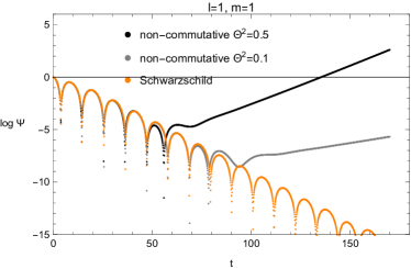
Figure 9: The evolution of the mode function of the massless test scalar field for the case $l=m=1$. The left panel shows the 3D evolution of the mode function with $\Theta^{2}=0.5$. The right panel shows the time evolution of the mode function on constant radius $r^{*}$. The black curve is for $\Theta^{2}=0.5$, the gray curve for $\Theta^{2}=0.1$, and the orange curve corresponds to the standard Schwarzschild black hole.

In FIG. 9, we present an example of the evolution of the mode function of the massless test scalar field for the case of $l=m=1$. In the left panel, we show the 3D evolution of the massless test scalar field for the case of $\Theta^{2}=0.1$. In the right panel, we show the time evolution of mode function located at constant $r^{*}$. The black line stands for the deformed Schwarzschild solution with $\Theta^{2}=0.5$, the gray line stands for $\Theta^{2}=0.1$, and orange line stands for the standard Schwarzschild black hole solution. From FIG. 9, it is obvious that the QNM ringing of the deformed Schwarzschild solution is nearly the same as that of the standard Schwarzschild black hole. This means that the system has nearly the same QNM frequencies as the standard Schwarzschild black hole solution. However, the long time evolution of this solution is very different from that of the standard Schwarzschild black hole. In addition, it is evident that for longer time evolution, the massless scalar field in the deformed Schwarzschild black hole gets constantly amplified, and this means that this scalar perturbation is not stable.

IV.4 A toy effective potential

In order to understand the growing behavior of the mode function mentioned in the previous subsection, we constructed a toy effective potential to grasp some intuitive knowledge. The toy effective potential is constructed as

$$V_{\mathrm{toy}}(r^{*})=\left\{\begin{aligned} &-0.00700034\;&r<-8.6\\ &0.1+0.0124419r\;&-8.6<r<0\\ &0.1-0.0106667r\;&0<r<6\\ &1.29599\frac{1}{r^{2}}\;&r>6\end{aligned}\right.~{}.$$ (48)

The toy effective potential is constructed in order to grasp the overall shape and the asymptotic behavior of the effective potential we have, while the details around the peak are not fully kept. In FIG. 10, the toy effective potential is plotted and compared with the effective potential of the deformed Schwarzschild black hole for the case of $l=m=1$ and $\Theta^{2}=0.5$ in NC gravity.

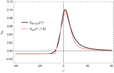
Figure 10: A comparison of the shape of the toy effective potential that we have constructed with the exact effective potential for the case of $l=m=1$ and $\Theta^{2}=0.5$.

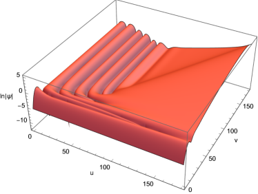
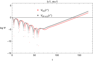
Figure 11: The evolution of the massless scalar field with the toy effective potential (48). The left panel shows the 3D evolution of the massless scalar field with the toy effective potential. The right panel shows the time evolution of the test scalar field located at constant radius. The pink curve stands for the case of toy effective potential, while the gray curve stands for the exact effective potential for $l=m=1$ and $\Theta^{2}=0.5$.

In addition, we solve the Schr$\ddot{\text{o}}$dinger-like equation employing the toy effective potential we constructed here, and the result is shown in FIG. 11. The left panel shows the 3D evolution of the massless scalar field governed by the toy effective potential. The right panel shows the time evolution of the massless scalar field located at constant radius. The pink line stands for the case of the toy effective potential, while the gray line stands for the case of the effective potential of the deformed Schwarzschild black hole for the case of $l=m=1$ and $\Theta^{2}=0.5$. From FIG. 11, we can easily see that the toy effective potential imitates quite well the long time behavior of the effective potential of the deformed Schwarzschild black hole.

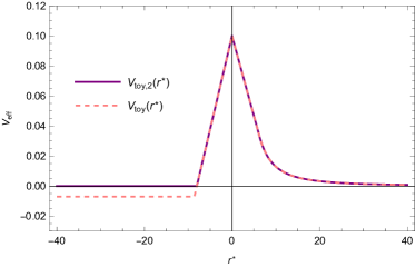
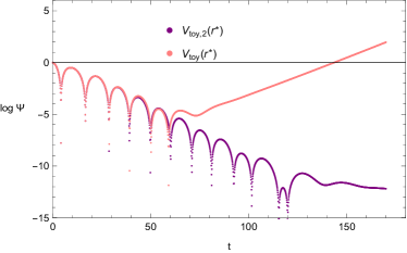
Figure 12: A comparison of the toy effective potential, which has zero asymptotic value, with the toy effective potential which has negative asymptotic value. The left panel compares the shapes of these two effective potentials, while the right panel shows the time evolution of the test scalar field governed by the two effective potentials.

In order to understand how the overall shape and asymptotic value affect the shape of the time evolution behavior of the massless scalar field, we construct another toy effective potential nearly the same with the previous one, but with zero asymptotic value on the negative side. In FIG. 12, we compare these two toy effective potentials. In the left panel, we show the shape of these two toy effective potentials. In the right panel, we show the time evolution of the massless scalar field governed by these two toy effective potentials, located at constant radius. It is easily seen that for the QNM ringing period, the two toy effective potentials give nearly the same time evolution behavior. However, the long time evolution of the two toy effective potentials are quite different. For the toy effective potential with zero asymptotic value, the scalar perturbation is stable, while for the one with negative asymptotic value, the scalar perturbation gets continuously amplified and is unstable. This leads us to the conclusion that the unstable time evolution of the massless scalar field is tightly related to the behavior of effective potential close to the event horizon.

V Conclusions

In this work we have calculated the Quasinormal Modes frequencies of a massless test scalar field around static black holes solutions in Noncommutative gravity. As a first step we obtained the master equation, which is of a Schr$\ddot{\text{o}}$dinger-like form and, thus, the effective potential was explicitly written. The effective potential is made of three parts: (i) the Schwarzschild effective potential, i.e. $V_{\mathrm{sch}}$, (ii) the contribution from the $j=0$ part, i.e. $V_{0}$, and (iii) the contribution from the $j>0$ part, i.e. $V_{j}$. In order for these parts to be computed we excluded the polar orbits ($m=0$) in order to avoid a divergence due to the fact that the deformed Schwarzschild black hole is “broken” at the poles. Furthermore, a tortoise coordinate was employed in order to make the computation of the effective potential easier, and additionally a discretization method was used.

Using several diagrams and two toy effective potentials, we have shown that Noncommutative gravity does have an effect on the Quasinormal Modes evolution compared to the one obtained in the framework of General Relativity. In particular, in the long time evolution of the massless scalar field, due to the Noncommutative corrections the stability of the scalar pertubations is missed.

Our results are relevant in the perspective of increasing accuracy in observations of gravitational waves from binary gravitational systems, whose characteristic oscillation modes can provide interesting information. Furthermore, the analysis performed in this paper could be used as an additional tool to test the General Relativity predictions and examine whether gravitational modifications of the specific form induced by Noncommutative geometry are possible.

Appendix A The first-order operator $\mathcal{D}_{(1)m,\omega}^{2}$

The first order operator $\mathcal{D}_{(1)m,\omega}^{2}$ in (29) is given by ChenTsao

$$\mathcal{D}_{(1)m,\omega}^{2} =\frac{m^{2}{\cal F}}{r^{2}\sin^{2}\theta}\left(A_{j}-D_{j}\right)\cos^{j}\theta-\frac{{\cal F}}{r^{2}}\left(A_{i}-B_{j}\right)\cos^{j}\theta\left[\partial_{r}\left(r^{2}{\cal F}\partial_{r}\right)\right]-\frac{{\cal F}^{2}}{2}\left(A_{j}^{\prime}-B_{j}^{\prime}+C_{j}^{\prime}+D_{j}^{\prime}\right)\cos^{j}\theta\partial_{r}$$

$$-\frac{{\cal F}}{r^{2}}\left(A_{j}-C_{j}\right)\cos^{j}\theta\left(\cot\theta\partial_{\theta}+\partial_{\theta}^{2}\right)-\frac{{\cal F}}{2r^{2}}\left[\left(A_{j}+B_{j}-C_{j}+D_{j}\right)\partial_{\theta}\cos^{j}\theta\right]\partial_{\theta}-\frac{2i\omega{\cal F}}{r}a_{j}\cos^{j}\theta\left(r\partial_{r}+1\right)$$

$$-i\omega{\cal F}\partial_{r}a_{j}\cos^{j}\theta-\frac{2i\omega}{r^{2}}b_{j}\cos^{j}\theta\partial_{\theta}-\frac{i\omega}{r^{2}\sin\theta}b_{j}\partial_{\theta}\left(\cos^{j}\theta\sin\theta\right)-\frac{im{\cal F}}{r^{2}\sin^{2}\theta}\left[2d_{j}\cos^{j}\theta{\cal F}\partial_{r}+\partial_{r}\left({\cal F}d_{j}\right)\cos^{j}\theta\right]$$

$$+\frac{im{\cal F}}{r^{4}\sin^{3}\theta}e_{j}\left(j\cos^{j-1}\theta\sin^{2}\theta+\cos^{j+1}\theta\right)-\frac{2im{\cal F}}{r^{4}\sin^{2}\theta}e_{j}\cos^{j}\theta\partial_{\theta}$$

$$+\frac{{\cal F}}{r^{2}}\left[\partial_{r}\left({\cal F}c_{j}\right)\cos^{j}\theta\partial_{\theta}+2{\cal F}c_{j}\cos^{j}\theta\partial_{r\theta}^{2}\right]+\frac{{\cal F}^{2}}{r^{2}\sin\theta}c_{j}\partial_{\theta}\left(\cos^{j}\theta\sin\theta\right)\partial_{r}\,.$$ (49)

The summations over $j$ are implicitly assumed in each term.

Appendix B The coefficients of the effective potential (35)

The coefficients $a^{j}_{lm},....,h^{j}_{lm}$ of the effective potential (35) are given as ChenTsao

$$a^{j}_{lm} =\frac{m^{2}}{\mathcal{N}_{lm}}\int_{-1}^{1}\frac{x^{j}\left({P_{l}^{m}}\right)^{2}}{1-x^{2}}dx\,,$$ (50)

$$b^{j}_{lm} =\frac{1}{\mathcal{N}_{lm}}\int_{-1}^{1}x^{j}\left({P_{l}^{m}}\right)^{2}dx\,,$$ (51)

$$c^{j}_{lm} =\frac{1}{\mathcal{N}_{lm}}\int_{-1}^{1}x^{j}{P_{l}^{m}}\left[\left(1-x^{2}\right)\partial_{x}^{2}-2x\partial_{x}\right]{P_{l}^{m}}dx\,,$$ (52)

$$d^{j}_{lm} =\frac{1}{\mathcal{N}_{lm}}\int_{-1}^{1}{P_{l}^{m}}\left(1-x^{2}\right)\left(\partial_{x}x^{j}\right)\left(\partial_{x}{P_{l}^{m}}\right)dx\,,$$ (53)

$$e^{j}_{lm} =\frac{-1}{\mathcal{N}_{lm}}\int_{-1}^{1}dxx^{j}{P_{l}^{m}}\sqrt{1-x^{2}}\partial_{x}{P_{l}^{m}}\,,$$ (54)

$$f^{j}_{lm} =\frac{1}{\mathcal{N}_{lm}}\int_{-1}^{1}dx\left({P_{l}^{m}}\right)^{2}\left[\frac{x^{j+1}}{\sqrt{1-x^{2}}}-\sqrt{1-x^{2}}\partial_{x}x^{j}\right]\,,$$ (55)

$$g^{j}_{lm} =\frac{m}{\mathcal{N}_{lm}}\int_{-1}^{1}\frac{x^{j}\left({P_{l}^{m}}\right)^{2}dx}{1-x^{2}}\,,$$ (56)

$$h^{j}_{lm} =\frac{m}{\mathcal{N}_{lm}}\int_{-1}^{1}\frac{\left({P_{l}^{m}}\right)^{2}dx}{\left(1-x^{2}\right)^{3/2}}\left[jx^{j-1}\left(1-x^{2}\right)+x^{j+1}\right]+\frac{2m}{\mathcal{N}_{lm}}\int_{-1}^{1}\frac{x^{j}{P_{l}^{m}}\left(\partial_{x}{P_{l}^{m}}\right)dx}{\sqrt{1-x^{2}}}$$ (57)

with

$$\int_{-1}^{1}dxP^{m}_{l}(x)P^{m}_{k}(x)=\frac{2(l+m)!}{(2l+1)(l-m)!}\,\delta_{lk}\,,$$ (58)

and

$$\mathcal{N}_{lm}\equiv\frac{2(l+m)!}{(2l+1)(l-m)!}.$$ (59)

References

- (1) H. Snyder, Phys. Rev. 71, 38 (1947).
- (2) N. Seiberg and E. Witten, J. High Energy Phys. 09, 32 (1999).
- (3) L. Alvarez-Gaumé and M.A. Vazquez-Mozo, Nucl. Phys. B 668, 293 (2003).
- (4) S. Carroll, J. Harvey, V.A. Kostelecky, C. Lane, and T. Okamoto, Phys. Rev. Lett. 87, 141601 (2001).
- (5) M. Chaichian, K. Nishijima, and A. Tureanu, Phys. Lett. B 568, 146 (2003).
- (6) S. Doplicher, in Proceedings of the 37th Karpacz Winter School of Theoretical Physics, 2001, p. 204, hep-th/0105251.
- (7) S. Doplicher, K. Fredenhagen, and J.E. Roberts, Commun. Math. Phys. 172, 187 (1995).
- (8) D. Bahns, S. Doplicher, K. Fredenhagen, and G. Piacitelli, Phys. Lett. B 533, 178 (2002).
- (9) A. Iorio and T. Sykora, Int. J. Mod. Phys. A 17, 2369 (2002).
- (10) R. Jackiw, Phys. Rev. Lett. 41, 1635 (1978).
- (11) R. Jackiw and S.Y. Pi, Phys. Rev. Lett. 88, 111603 (2002).
- (12) G. Amelino-Camelia, G. Mandanici, and K. Yoshida, JHEP 01, 037 (2004).
- (13) Z. Guralnik, R. Jackiw, S.Y. Pi, and A.P. Polychronakos, Phys. Lett. B 517, 450 (2001).
- (14) R. G. Cai, Phys. Lett. B 517, 457 (2001)
- (15) M. R. Douglas and N. A. Nekrasov, Rev. Mod. Phys. 73, 977 (2001).
- (16) R. J. Szabo, Phys. Rep. 378, 207 (2003).
- (17) A.A. Bichl, J.M. Grimstrup, H. Grosse, E. Kraus, L. Popp, M. Schweda, and R. Wulkenhaar, Eur. Phys. J. C 24, 165 (2002).
- (18) J.M. Grimstrup, B. Kloibock, L. Popp, V. Putz, M. Schweda, and M. Wickenhauser, Int. J. Mod. Phys. A 19, 5615-5624 (2004).
- (19) M.R. Douglas and N.A. Nekrasov, Rev. Mod. Phys. 73, 977 (2001).
- (20) H. Omori, Y. Maeda, N. Miyazaki, and A. Yoshioka, Lett. Math. Phys. 82 153 (2007).
- (21) F. Ardalan, H. Arfaei, and M. M. Sheikh-Jabbari, J. High Energy Phys. 02 (1999) 016.
- (22) O. F. Dayi and B. Yapiskann, J. High Energy Phys. 10 (2002) 022.
- (23) S. Ghosh, Nucl. Phys. B670, 359 (2003).
- (24) B. Chakraborty, S. Gangopadhyay, and A. Saha, Phys. Rev. D 70, 107707 (2004).
- (25) S. Ghosh, Phys. Rev. D 70, 085007 (2004).
- (26) P. Mukherjee and A. Saha, Mod. Phys. Lett. A 21, 821 (2006).
- (27) A. Saha, A. Rahaman, and P. Mukherjee, Phys. Lett. B 638, 292 (2006).
- (28) X. Calmet and A. Kobakhidze, Phys. Rev. D 72, 045010 (2005).
- (29) M. Chaichian, P. Presnajder, M.M. Sheikh-Jabbari, and A. Tureanu, Eur. Phys. J. C 29, 413 (2003).
- (30) M. Chaichian, A. Kobakhidze, and A. Tureanu, Eur. Phys. J. C 47, 241 (2006).
- (31) X. Calmet, B. Jurco, P. Schupp, J. Wess, and M. Wohlgenannt, Eur. Phys. J. C 23, 363 (2002).
- (32) P. Aschieri, B. Jurco, P. Schupp, and J. Wess, Nucl. Phys. B651, 45 (2003).
- (33) M. Chaichian, A. Tureanu, R.B. Zhang, X. Zhang, J. Math. Phys. 49, 073511 (2008).
- (34) G. Manolakos, P. Manousselis and G. Zoupanos, JHEP 08, 001 (2020).
- (35) G. Manolakos, P. Manousselis, D. Roumelioti, S. Stefas and G. Zoupanos, Universe 8, no.4, 215 (2022).
- (36) A.H. Chamseddine, Phys. Lett. B 504, 33 (2001).
- (37) L. Bonora, M. Schnabl, M. Sheikh-Jabbari, A. Tomasiello, Nucl. Phys. B 589, 461 (2000).
- (38) B. Jurco, S. Schraml, P. Schupp, J. Wess, Eur. Phys. J. C 17, 521 (2000).
- (39) M. Chaichian, P.P. Kulish, K. Nishijima, A. Tureanu, Phys. Lett. B 604, 98 (2004).
- (40) M. Chaichian, P. Prešnajder, A. Tureanu, Phys. Rev. Lett. 94, 151602 (2005).
- (41) P. Aschieri, C. Blohmann, M. Dimitrijevic, F. Meyer, P. Schupp, J. Wess, Class. Quant. Grav. 22, 3511 (2005).
- (42) L. Álvarez-Gaumé, F. Meyer, M.A. Vazquez-Mozo, Nucl. Phys. B 75, 392 (2006).
- (43) X. Calmet, A. Kobakhidze, Phys. Rev. D 72, 045010 (2005).
- (44) X. Calmet, A. Kobakhidze, Phys. Rev. D 74, 047702 (2006).
- (45) A. Kobakhidze, Int. J. Mod. Phys. A 23, 2541 (2008).
- (46) M. Chaichian, A. Tureanu, Phys. Lett. B 637, 199 (2006).
- (47) M. Chaichian, A. Tureanu, G. Zet, Phys. Lett. B 660, 573 (2008).
- (48) H.-P. Nollert, Class. Quant. Grav. 16, R159 (1999).
- (49) R. A. Konoplya and A. Zhidenko, Rev. Mod. Phys. 83, 793 (2011).
- (50) M. Isi and W. M. Farr, arXiv:2107.05609 [gr-qc].
- (51) Y.F. Cai, G. Cheng, J. Liu, M. Wang, and H. Zhang, JHEP 01, 108 (2016).
- (52) V. Cardoso, A. Maselli, E. Berti, C. F. B. Macedo and R. McManus, Phys. Rev. D 99, 104077 (2019).
- (53) R. McManus, E. Berti, C. F. B. Macedo, M. Kimura, A. Maselli, and V. Cardoso, Phys. Rev. D 100, 044061 (2019).
- (54) G. Guo, P. Wang, H. Wu, and H. Yang, JHEP 06, 060 (2022).
- (55) A. Ejlli, D. Ejlli, A. M. Cruise, G. Pisano and H. Grote, Eur. Phys. J. C 79, no.12, 1032 (2019).
- (56) Akiyama et al. (Event Horizon Telescope Coll.), Astrophys. J. Lett. 875, L1 (2019).
- (57) Akiyama et al. (Event Horizon Telescope Coll.), Astrophys. J. Lett. 875, L6 (2019).
- (58) Psaltis et al. (Event Horizon Telescope Coll.), Phys. Rev. Lett. 125, 141104 (2020).
- (59) Abbott et al. (LIGO Scientific, Virgo Coll.), Phys. Rev. Lett. 116, 061102 (2016).
- (60) Abbott et al. (LIGO Scientific, Virgo Coll.), Phys. Rev. Lett. 116, 221101 (2016).
- (61) Y.-F. Cai, C. Li, E. N. Saridakis, L. Xue, Phys. Rev. D 97, 103513 (2018).
- (62) C. Li, L. Xue, X. Ren, Y.-F. Cai, D. A. Easson, Y.-F. Yuan, and H. Zhao, Phys. Rev. Res. 2, 023164 (2020).
- (63) C. Li, H. Zhao, and Y.-F. Cai; Phys. Rev. D 104, 064027 (2021).
- (64) K. Jusufi, M. Azreg-Aïnou, M. Jamil and E. N. Saridakis, Universe 8, no.2, 102 (2022).
- (65) F. J. Zerilli, Phys. Rev. Lett. 24, 737 (1970).
- (66) S. Chandrasekhar and S. L.Detweiler, Proc. Roy. Soc. Lond. A 344, 441 (1975).
- (67) K. D. Kokkotas and B. G. Schmidt, Living Rev. Rel. 2, 2 (1999).
- (68) E. Berti, V. Cardoso and A. O. Starinets, Class. Quant. Grav. 26 163001 (2009).
- (69) Y. Hatsuda, M. Kimura, Universe 7, 476 (2021).
- (70) O. Dreyer, B. J. Kelly, B. Krishnan, L.S. Finn, D. Garrison and R. Lopez-Aleman, Class. Quant. Grav. 21, 787 (2004).
- (71) E. Berti, V. Cardoso, and C. M. Will, Phys. Rev. D 73, 064030 (2006).
- (72) W. Isi, M. Giesler, W.M. Farr, M. A. Scheel and S. A. Teukolsky, Phys. Rev. Lett. 123, 111102 (2019).
- (73) P.A. Cano, K. Fransen, T. Hertog, and S. Maenaut, Phys. Rev. D 105, 024064 (2022).
- (74) B. Wang, C.-Y. Lin, and C. Molina, Phys. Rev. D 70, 064025 (2004).
- (75) J. L. Blázquez-Salcedo, C. F. B. Macedo, V. Cardoso, V. Ferrari, L. Gualtieri, F.S. Khoo, J. Kunz, and P. Pani, Phys. Rev. D 94, 104024 (2016).
- (76) R. Penco, L. Santoni and E. Trincherini, JHEP 02, 127 (2019).
- (77) R: Bécar, P. A. González, E. Papantonopoulos, and Y. Vásquez, Eur. Phys. J. C 80 600 (2020).
- (78) A. Aragón, P.A. Gonzalez, E. Papantonopoulos, Y. Vásquez, Eur. Phys. J. C 81, 407 (2021).
- (79) H. Liu, Y. Liu, B. Wang, and J.P. Wu, Phys. Rev. D 103, 024006 (2021).
- (80) T. Karakasis, E. Papantonopoulos, C. Vlachos, Phys. Rev. D 105 024006 (2022).
- (81) P. A. González, E. Papantonopoulos, J. Saavedra and Y. Vásquez, JHEP 06, 150 (2022).
- (82) A. Ishibashi and H. Kodama, Prog. Theor. Phys. 110 901 (2003).
- (83) Y. Zhao, X. Ren, A. Ilyas, E. N. Saridakis and Y. F. Cai, JCAP 10, 087 (2022).
- (84) A. Chowdhury, S. Devi, and S. Chakrabarti, Phys. Rev. D 106, no.2, 024023 (2022).
- (85) J. Madore, S. Schraml, P. Schupp, and J. Wess, Eur. Phys. J. C 16, 161 (2000).
- (86) I. Mocioiu, M. Pospelov, and R. Roiban, Phys. Lett. B 489, 390 (2000).
- (87) M. Chaichian, M. M. Sheikh-Jabbari and A. Tureanu, Phys. Rev. Lett. 86, 2716 (2001).
- (88) M. Chaichian, M. M. Sheikh-Jabbari and A. Tureanu, Eur. Phys. J. C 36, 251 (2004).
- (89) P. K. Joby, P. Chingangbam, and S. Das, Phys Rev D 91, 083503 (2015).
- (90) S. M. Carroll, J. A. Harvey, V. A. Kostelecky, C. D. Lane, and T. Okamoto, Phys. Rev. Lett. 87, 141601 (2001).
- (91) X. Calmet, Eur. Phys. J. C 41, 269 (2005).
- (92) P. Joby, P. Chingangbam, and S. Das, Phys. Rev. D 91, 083503 (2015).
- (93) X. Calmet and C. Fritz, Phys. Lett. B 747, 406 (2015).
- (94) G. Lambiase, G. Vilasi, A. Yoshioka, Class. Quant. Grav. 34, 025004 (2017).
- (95) A. Addazi, J. Alvarez-Muniz, R. Alves Batista, G. Amelino-Camelia, V. Antonelli, et al. Prog. Part. Nucl. Phys. 125, 103948 (2022).
- (96) A. Kobakhidze, C. Lagger, and A. Manning, Phys. Rev. D94, 064033 (2016).
- (97) A. Kobakhidze, Phys. Rev. D79, 047701 (2009).
- (98) P. Aschieri, C. Blohmann, M. Dimitrijevic, F. Meyer, P. Schupp, and J. Wess, Class. Quant. Grav. 22, 3511 (2005).
- (99) X. Calmet and A. Kobakhidze, Phys. Rev. D 72, 045010 (2005).
- (100) P. Aschieri, M. Dimitrijevic, F. Meyer, and J. Wess, Class. Quant. Grav. 23, 1883 (2006).
- (101) A. Kobakhidze, Int. J. Mod. Phys. A 23, 2541 (2008).
- (102) R. J. Szabo, Class. Quant. Grav. 23, R199 (2006).
- (103) X. Calmet and A. Kobakhidze, Phys. Rev. D 74, 047702 (2006).
- (104) P. Mukherjee and A. Saha, Phys. Rev. D 74, 027702 (2006).
- (105) T. Kanazawa, G. Lambiase, G. Vilasi, A. Yoshioka, Eur. Phys. J. C 79, 95 (2019).
- (106) E. N. Saridakis et al. [CANTATA], [arXiv:2105.12582 [gr-qc]].
- (107) S. M. Carroll, J. A. Harvey, V. A. Kostelecky, C. D. Lane and T. Okamoto, Phys. Rev. Lett. 87, 141601 (2001).
- (108) M. Chaichian, A. Tureanu, R.B. Zhang, X. Zhang, J. Math. Phys. 49, 073511 (2008).
- (109) D. Wang, R.B. Zhang, X. Zhang, Class. Quant. Grav. 26, 085014 (2009).
- (110) D. Wang, R.B. Zhang, X. Zhang, Eur. Phys. J. C 64, 439 (2009).
- (111) W. Sun, D. Wang, N. Xie, R.B. Zhang, X. Zhang, Eur. Phys. J. C 69, 271 (2010).
- (112) M. Chaichian, A. Tureanu, M.R. Setare, G. Zet, JHEP04, 064 (2008).
- (113) D.V. Singh, M.S. Ali, S.G. Ghosh, Int. J. Mod. Phys.D 27, 1850108 (2018).
- (114) S.A. Alavi and S. Nodeh, Phys. Scr. 90, 035301 (2015).
- (115) C. Y. Chen, H. W. Chiang and J. S. Tsao, Phys. Rev. D 106 (2022) no.4, 044068.