Non-Uniqueness in Plane Fluid Flows

Abstract

Examples of dynamical systems proposed by Z. Artstein and C. M. Dafermos admit non-unique solutions that track a one parameter family of closed circular orbits contiguous at a single point. Switching between orbits at this single point produces an infinite number of solutions with the same initial data. Dafermos appeals to a maximal entropy rate criterion to recover uniqueness.

These results are here interpreted as non-unique Lagrange trajectories on a particular spatial region. The corresponding velocity is proved consistent with plane steady compressible fluid flows that for specified pressure and mass density satisfy not only the Euler equations but also the Navier-Stokes equations for specially chosen volume and (positive) shear viscosities. The maximal entropy rate criterion recovers uniqueness.

Key words: Non-uniqueness, entropy rate criterion, Euler equations, Navier-Stokes equations.
MSC classes: 76N10 (primary), 34A12, 35Q35 (secondary).

1 Introduction

This paper derives explicit non-unique continuous Lagrange trajectories related to certain Euler and Navier-Stokes steady compressible plane fluid flow. The orbits tracked by the trajectories belong to a one parameter family of closed contiguous circular paths. Non-uniqueness occurs when trajectories switch orbits at the common point of intersection. Even so, uniqueness follows for the problems considered here by appeal to an entropy rate criterion that isolates a single preferred trajectory.

The non-unique behaviour is not dissimilar to that occurring in the convex integration investigations by De Lellis and Szèkelyhidi [8, 9] and Buckmaster and Vicol [4] for the incompressible Euler and Navier-Stokes systems. It is therefore reasonable to speculate whether a unique solution also might be selected by application of an entropy rate criterion. Brief comment on this aspect is given in Section 5.

The present analysis is partly inspired by an example in control theory proposed by Artstein [1, see eqn. (6.1)] who, rather than non-uniqueness, emphasises non-existence of suitable controls that otherwise stabilise the system and ensure solutions asymptotically approach zero. The primary motivation, however, comes from what Dafermos [7] refers to as an artificial example of a nonlinear oscillator governed by an ordinary differential equation. The associated trajectories considered by both Artstein and Dafermos are circular, and touch at their common point of intersection taken to be the origin. Consequently, trajectories can be switched at the origin by instantaneous variation of an entropy function that is constant along individual trajectories. In this manner, irrespective of initial conditions, an uncountable set of different solutions can be chosen to establish non-uniqueness.

Dafermos [7] recovers uniqueness by selecting that particular solution which dissipates entropy at maximum rate. Such a solution is not only unique but physically relevant in the sense of Hadamard’s definition of well-posedness. Similar entropy rate criteria, originally formulated to treat shock wave propagation, include the maximal entropy rate proposed by Ziegler [23] and the minimum entropy rate due to Prigogine [18, Chapt. V]. Both principles are reviewed in the monograph by Moroz [16, Chapt. 1]. Glimm, Lazarev and Chen [12] remark that the subtle difference between these two principles may cause confusion. Ziegler’s principle is relevant to closed thermodynamic systems while Prigogine’s principle applies to open thermodynamic systems. Evidently, Dafermos’s investigation relates to a closed system.

Dafermos’s example, however, is far from trivial. It is shown in this paper that solutions, interpreted as steady Lagrange trajectories (particle paths), are related to steady plane flows for compressible Euler and Navier-Stokes equations with variable mass density and positive shear viscosity. The extension to fluid problems demonstrates that tracking arbitrarily prescribed discrete entropy profiles produces an infinite number of continuous Lagrange trajectories with the same initial conditions. Consequently, trajectories are not unique. Nevertheless, a single unique trajectory is identified by the maximal entropy rate admissibility criterion proposed by Dafermos [7]. An interpretation of this result is that “wild” initial data can be produced for steady solutions to an initial boundary problem for both the Euler and Navier-Stokes equations. The term “wild” is understood in the sense that there are an infinite number of Lagrange trajectories for the same initial conditions. The entropy rate criterion identifies a unique trajectory and renders the notion of “wildness” redundant.

The conclusion contrasts with the uniqueness results for weak solutions to the incompressible Navier-Stokes equations obtained by Robinson and Sadowski [19, 20]. These authors show for sufficiently regular velocity that the Lagrange trajectories are unique and smooth in time for almost every initial data. On the other hand, the velocity for the Lagrange trajectories considered here lacks Lipschitz continuity at one point and therefore does not satisfy the continuity conditions imposed by Robinson and Sadowski.

An alternative admissibility procedure, introduced by Brenier [3], relies upon the concave maximization of a certain functional to derive smooth solutions to Euler’s equation. Further procedures include that by Lasarzik [14] who adopts a maximal entropy rate to conclude that “dissipative solutions” as defined by P.-L. Lions [15] exist, are unique, and depend continuously upon initial data for both the Euler and Navier-Stokes equations of incompressible fluid dynamics. It must be noted, however, that such dissipative solutions are not in general weak solutions. A different notion of dissipative solution is treated by Breit, Feireisl and Hofmanova [2] who replace the concept of a weak solution by a semi-flow satisfying a maximal entropy rate production criterion. By construction, the semi-flow implies modified well-posedness of the Euler system.

Also of importance is whether the maximal entropy rate criterion can be accurately simulated by numerical analysis. Glimm, Lazarev and Chen [12] note that this comparatively delicate issue is of substantial physical importance. A numerical method that preserves qualitative behaviour is required and, in fact, it is shown in Section 4 that the symplectic Euler method successfully ensures convergence to the unique solution selected by the criterion. The explicit Euler method fails in this respect.

As already remarked, based upon the Artstein-Dafermos examples, the non-uniqueness described in this paper for the Euler and Navier-Stokes equations is due to the corresponding Lagrange trajectories switching at the origin from one circular path to another along each of which there is different constant entropy. Arbitrary prescription of these entropies and the order in which the trajectories are described results in an uncountable number of distinct solutions satisfying the same initial conditions. The behaviour has features in common with that respectively established by De Lellis and Szèkelyhidi [8, 9] and by Buckmaster and Vicol [4] for weak solutions on a torus to the incompressible Euler and Navier-Stokes equations. These authors use convex integration techniques to prove that an arbitrary number of such weak solutions exist possessing both the same assigned smooth global energy and the same initial conditions. Consequently, non-uniqueness is established. (Extension to the compressible Euler equations is due to Chiodaroli and Kreml [6], and to Feireisl [11]).

Arbitrary specification of an appropriate profile is thus common to both developments and invites exploration of the possible application of a maximal entropy rate criterion to identify a unique solution from among the many weak solutions determined by convex integration methods.

Of separate interest is the physical relevance of weak solutions obtained by convex integration to the Euler and Navier-Stokes equations. Such solutions are the limit of increasingly high frequency oscillatory perturbations that eventually may contravene the basic continuum hypotheses assumed in the derivation of the equations. In this respect, the Lagrange trajectories considered here are explicit and indeed are continuously differentiable except at the origin. Clearly, apart from this singularity, they accord with continuum hypotheses.

Section 2 commences with Dafermos’s construction of non-unique orbits for a nonlinear oscillator that involves the arbitrary prescription of an entropy function constant on each path. A theorem conveniently summarises relevant conclusions. Two admissibility criteria proposed by Dafermos are then described that recover a physically meaningful unique trajectory. The first criterion augments the system of equations by a friction term. Solutions to the penalised system tend to a unique solution in the limit as friction tends to zero. The second, or maximal entropy rate, criterion requires maximum dissipation of the individual entropies as trajectories are successively switched and leads to the same path obtained by the limiting friction argument. Section 3 establishes that the velocity occurring in the nonlinear oscillator satisfies the plane compressible Euler equations with specified pressure and particular non-uniform mass density. Moreover, the corresponding Lagrange trajectories are geometrically similar to those obtained from the nonlinear oscillator and therefore possess similar non-uniqueness features. Isolation of a unique trajectory follows from the maximal entropy rate criterion. The analysis is extended to the corresponding plane compressible Navier-Stokes equations with specially chosen (positive) shear and volume viscosities. These viscosity coefficients are computed in the Appendices. Section 4 discusses the numerical approximations of solutions to the Dafermos system considered in Section 2. The objective is to employ a numerical method that not only preserves the qualitative behaviour of constant entropy along individual trajectories, but is also capable of simulating trajectories selected by the maximal entropy rate criterion. Convergence to a unique solution would then be implied. The symplectic Euler method satisfies these requirements since it determines the approximation to the entropy function to within an error of the order of the step size $h>0$. The approach is diagramatically illustrated and arguments are given that the discrete flow selects the solution given by the entropy rate admissibility criterion. Section 5 comments on the resemblance between the results of Section 3 and those in the convex integration literature that for a given smooth global energy construct an infinite number of solutions to the Euler equations on a torus. A final brief remark concerns the fundamental issue of whether the eventual irregularity of such solutions contravenes basic continuum hypotheses.

Standard notation is employed throughout the main text apart from Remark 3.1 where bold type indicates vectors. The Appendices introduce an indicial notation accompanied by the summation and comma conventions.

2 Motivation and admissibility criteria

This section reviews previous contributions that inspired the present generalisation to the Euler and Navier-Stokes equations. The discussion also explains how an entropy rate criterion recovers a unique solution.

Let $(x(t),y(t))\in\mathrm{I\!R\!}^{2},\,t\in\mathrm{I\!R\!},$ be state variables corresponding to the Cartesian coordinates of a point moving in the plane as time varies. Dafermos [7] studies motions whose state variables satisfy the system of ordinary differential equations for a nonlinear oscillator given by

$$\dot{x} = y,$$ (2.1)

$$\dot{y} = \frac{(y^{2}-x^{2})}{2x},$$ (2.2)

where a superposed dot indicates differentiation with respect to time $t$.

Initial data are specified by

$$(x(0),\,y(0))=(x_{0},\,y_{0}),$$ (2.3)

where $(x_{0},\,y_{0})$ are prescribed.

The velocity component (2.1) is continuously differentiable everywhere but the component (2.2) is not continuous at the origin. Dynamics are best understood from an integrated form of the equations given below.

It is immediate from (2.1) and (2.2) that the entropy function $H(x,y)$, defined by

$$H(x,y):=\frac{(x^{2}+y^{2})}{2x},$$ (2.4)

is invariant with respect to time $t$; that is

$$\frac{dH(x(t),y(t))}{dt}=0,$$ (2.5)

or

$$H(x,\,y)=c$$ (2.6)

for positive constant $c$.

Note that $H(x,y)$ is not to be confused with the (kinetic) energy. The relationship between these quantities is presented in Section 5.

The constant entropy function (2.4) implies that the state variables traverse the one parameter family of closed circular orbits

$$x^{2}+y^{2}=2xc.$$ (2.7)

Consequently,

$$(x-c)^{2}+y^{2}=c^{2},$$ (2.8)

and consequently $0\leq x(t)\leq 2c,\,-c\leq y(t)\leq c.$ Moreover, (2.1) implies that $x(t)$ increases or decreases as $y(t)$ is positive or negative so that the closed circular orbits are traversed clockwise. For varying $c\geq 1$ they touch each other at their common point of intersection located at the origin. Since solutions trace the family of orbits (2.8), equation (2.2) may be alternatively written as

$$\dot{y}=(c-x).$$ (2.9)

Artstein’s study [1, eqn. 6.1] is within the broader context of a control problem in which (2.1) and (2.9) are generalised to the family

$$\dot{x} = (2xy)w,$$ (2.10)

$$\dot{y} = (y^{2}-x^{2})w,$$ (2.11)

where $w(x,y)$ is a scalar control chosen to ensure stabilisability of the equilibrium state $x=y=0.$ It follows immediately that since

$$\frac{dx}{2xy}=\frac{dy}{(y^{2}-x^{2})},$$ (2.12)

the paths followed by solutions to (2.10) and (2.11) are given by the family of circular closed orbits (2.8) or alternatively (2.7), and consequently the function $H(x,t)$ is constant along each path. Dependent upon the choice of $w$, the Lipschitz condition may fail which would imply lack of uniqueness for paths with given initial data and which we now examine.

Particular choices of the control function $w(x,y)$ deserve attention.

First, set

$$w=x^{-\alpha},\qquad\alpha>0.$$ (2.13)

Substitution in (2.10) and (2.11) after appeal to (2.7) yields

$$\dot{x} = 2x^{(\frac{3}{2}-\alpha)}(2c-x)^{1/2},$$ (2.14)

$$\dot{y} = 2x^{(1-\alpha)}(c-x).$$ (2.15)

Hence (2.7), (2.14) represent an integrated form of (2.10), (2.14) where conservation of $H$ given (2.6) is extended by continuity to the origin. It is here that lack of Lipschitz continuity of the right hand side of (2.14) makes itself apparent and the usual loss of uniqueness occurs in $x$ for $1\leq\alpha<3/2$ (see, for example, Burkill [5]), while $y$ is well defined from the choice of $x$. As stated below, $\alpha=1$ is the value adopted by Dafermos [7].

As second choice, put

$$w=\frac{1}{2x^{2}},$$ (2.16)

to obtain from (2.10) and (2.11) the Hamiltonian system

$$\dot{x} = \frac{y}{x},$$ (2.17)

$$\dot{y} = \frac{(y^{2}-x^{2})}{2x^{2}},$$ (2.18)

whose Hamiltonian is the function $H(x,y)$.

Finally, consider

$$w=\frac{1}{2x}$$ (2.19)

which reduces (2.10) and (2.11) to the system (2.1) and (2.2) considered by Dafermos [7]. Explicit solutions, of interest when interpreted in Section 3 as Lagrange trajectories, are easily derived. Details are presented in Appendix A. Express (2.8) as

$$\dot{x}(t)=y(t)=\pm\sqrt{x(2c_{0}-x)},$$

where $c$ has assumed the particular value $c_{0}$ specified from initial data according to

$$c_{0}=\frac{(x_{0}^{2}+y_{0}^{2})}{2x_{0}}.$$ (2.20)

It is supposed that initial data are such that $c_{0}\geq 1.$ Choose the positive square root to obtain by integration

$$x(t)-c_{0}=c_{0}\cos{(-t+\theta_{0})}.$$ (2.21)

The corresponding expression for $y(t)$, obtained by differentiation of the last relation, becomes

$$y(t)=c_{0}\sin{(-t+\theta_{0})},$$ (2.22)

and shows that the constant $\theta_{0}$ is determined from initial data to be

$$\tan{\theta_{0}}=\frac{y_{0}}{x_{0}-c_{0}}.$$ (2.23)

The circular orbits (2.21) and (2.22) may otherwise be derived by integration of (2.1) and (2.9). They are centred at $(c_{0},0)$, where $c_{0}$ is determined from initial conditions (2.20), and are restricted to the set parametrized by $1\leq c_{0}\leq R$ sketched in Figure 1.

Figure 1: Phase portrait for (2.21) and (2.22).

Orbits tracked by the state variables, as predicted by (2.8), are centred at $(c_{0},\,0)$ and pass through the origin at times $(-t+\theta_{0})=-(2n+1)\pi,\,n=0,1,2,\ldots$ . Each circular orbit is completed in the same time $2\pi$ but at speeds dependent upon the radius:

$$\left(\dot{x}^{2}+\dot{y}^{2}\right)^{1/2}=c_{0},$$

corresponding to rigid body rotation.

Further properties are derived upon conversion to polar coordinates $(r,\theta)$. Set $x=r\cos{\theta},\,y=r\sin{\theta}$ so that (2.1) and (2.2) become

$$\dot{\theta} = -\frac{1}{2},$$ (2.24)

$$\dot{r} = \frac{1}{2}r\tan{\theta},$$ (2.25)

which by integration lead to

$$\theta(t) = -\frac{t}{2}+\theta_{0}/2,$$ (2.26)

$$r(t)\cos{(\theta_{0}/2)} = r_{0}\cos{\theta(t)},$$ (2.27)

where $\theta_{0}$ satisfies (2.23) and $(r_{0},\,\theta_{0}/2)$, the initial values of $(r(t),\,\theta(t))$, accordingly are given by

$$r_{0}=\left(x^{2}_{0}+y^{2}_{0}\right)^{1/2},\qquad\tan{(\theta_{0}/2)}=\frac{y_{0}}{x_{0}},$$

and

$$r_{0}=2c_{0}\cos{(\theta_{0}/2)}.$$

The last expression inserted into (2.27) gives

$$r(t)=2c_{0}\cos{\theta(t)},$$ (2.28)

which is the circular orbit previously obtained.

The state variables expressed by either (2.21) and (2.22), or by (2.26) and (2.28), indicate the explicit manner in which orbits pass through the origin $(0,0)$.

The calculations so far suppose that $c\geq 1$. To include the region $c<1$, Dafermos [7] considers the modified system

$$\dot{x} = y,\qquad\dot{y}=\frac{(y^{2}-x^{2})}{2x},\quad\mbox{for}\qquad(x-1)^{2}+y^{2}\geq 1,$$ (2.29)

$$\dot{x} = y,\qquad\dot{y}=(1-x),\qquad(x-1)^{2}+y^{2}<1.$$ (2.30)

Solutions to (2.30) are of the same form as (2.21) and (2.22) and indicate that corresponding trajectories move clockwise on circles

$$(x-1)^{2}+y^{2}=a^{2},\qquad a<1,$$ (2.31)

of radius $a<1$ centred at $(1,0)$ when $c<1$ in (2.6).

Of special interest is the circle of unit radius for which $a=c=1$.

Irrespective of prescribed initial conditions, each member of the family of orbits created by a sequence of different constants $c\geq 1$ possess the common property of lying in the positive half-plane and passing through the coordinate origin where they are mutually tangential. Dafermos [7] observes that global uniqueness of solutions to (2.1)-(2.2) is violated on allowing switching at the origin between orbits of different entropy levels $H(x,y)$ defined by (2.6). Specifically, a trajectory with initial conditions such that

$$H(x_{0},\,y_{0}):=\frac{(x^{2}_{0}+y^{2}_{0})}{2x_{0}}=c_{0}>1,$$ (2.32)

on reaching the origin switches to another trajectory for which

$$H(x,y)=c_{1}>1,\qquad c_{1}\neq c_{0}.$$ (2.33)

The composite trajectory is clearly continuous in the time variable $t$ and satisfies (2.29) for almost all $t$; in fact for all $t$ for which $(x(t),\,y(t))\neq(0,\,0)$. From (2.9) the jump in the acceleration $\ddot{x}=\dot{y}$ at the origin is given by

$$[\ddot{x}]_{(0,\,0)}=[\dot{y}]_{(0,\,0)}=c_{1}-c_{0}.$$ (2.34)

Hence, $\dot{y}$ is bounded for all $t$ and $y$ is Lipschitz continuous.

Trajectories for which $c<1$ remain interior to the circle of radius $1$ and do not pass through the origin. Consequently, switching is not possible.

The following theorem summarises for convenience these non-uniqueness results which are also applicable to the general control problem (2.10) and (2.11). In Section 5 the conclusion is compared to the non-uniqueness theorem of Buckmaster and Vicol [4] for the Navier-Stokes equations.

Figure 2: The region $\Omega=\Omega_{1}\cup\Omega_{2}$.

Theorem 2.1.

For $R>1$, define the plane region $\Omega=\Omega_{1}\cup\Omega_{2}$, depicted in Figure 2, by

$$\Omega_{1} := \left\{(x,y)\in\mathrm{I\!R\!}^{2}:1\leq(x-1)^{2}+y^{2},\,(x-R)^{2}+y^{2}\leq R^{2}\right\},$$ (2.35)

$$\Omega_{2} := \left\{(x,y)\in\mathrm{I\!R\!}^{2}:(x-1)^{2}+y^{2}<1\right\}$$ (2.36)

and let $e(t)$ denote the piece-wise constant function

$$e(t)=\begin{cases}c_{0},&0\leq t\leq t_{1},0\leq t_{1}<2\pi,\\ c_{n},&t_{n}=t_{1}+2(n-1)\pi\leq t<t_{n}+2\pi,\end{cases}$$ (2.37)

for $n=1,2,\dots$ and $0\leq t<\infty$.

Then for any sequence $c_{n}\geq 1$, there exists a Lipschitz continuous solution to (2.1) and (2.2). Trivially, the initial value problem with initial data $(x(0)=x_{0},\,y(0)=y_{0})\in\Omega_{1}$ possesses an infinite number of Lipschitz continuous solutions.

Dafermos [7] regains uniqueness by suggesting two admissibility criteria. The first asserts that the physically meaningful solution to (2.29) and (2.30) on $\Omega=\Omega_{1}\cup\Omega_{2}$ is the limit as $\gamma\rightarrow 0^{+}$ of solutions $(x_{\gamma},\,y_{\gamma})$ to the system with friction:

$$\dot{x}_{\gamma} = y_{\gamma},$$ (2.38)

$$\dot{y}_{\gamma} = g(x_{\gamma},\,y_{\gamma})-\gamma y_{\gamma},$$ (2.39)

where

$$g(x,y)=\begin{cases}\frac{(y^{2}-x^{2})}{2x},&(x-1)^{2}+y^{2}\geq 1,\\ (1-x),&(x-1)^{2}+y^{2}<1.\end{cases}$$

Solutions $(x_{\gamma},\,y_{\gamma})$ to (2.38) and (2.39) possess the limit $(x_{\gamma},\,y_{\gamma})\rightarrow(x,y)$ as $\gamma\rightarrow 0^{+}$ where

• $(x_{\gamma}(0),\,y_{\gamma}(0))\rightarrow(x_{0},\,y_{0})$ and

  $$c_{0}=\frac{(x^{2}_{0}+y^{2}_{0})}{2x_{0}}.$$

• The limit $(x,\,y)$ moves clockwise on the circle radius $c_{0}$ until it reaches the origin $x=0,\,y=0$.

• Upon reaching the origin, the solution switches once to the circle with entropy $e=1$ of radius $1$ centred at $(x,\,y)=(1,0)$. It remains on this circle moving clockwise.

The second criterion proposed by Dafermos is the entropy rate admissibility criterion which, although not applied directly to the present problem, requires that physically admissible solutions should have not only non-increasing entropy $e(t)$, but that the entropy should decrease at maximum possible rate. A simple illustration of the criterion for the system (2.29) and (2.30) is sketched in Figures 3-4 for possible entropy profiles (2.37).

Let $\delta>0$ and in Figure 3 select the point $\tau_{1}=t_{1}-\delta$ such that $0<\tau_{1}=t_{1}-\delta<t_{1}$ and $\tau_{1}$ lies within the first interval specified in (2.37) and therefore locates a point on the branch $e=c_{0}$.

Figure 3: Discrete energy profile.

Subsequent points given by $\tau_{n}=t_{1}-\delta+2\pi n,\,n=1,2,\ldots$ are chosen to lie in the interval $(t_{n},t_{n}+2\pi)$ so that $\tau_{n}$ is a point on $e=c_{n}$. On joining the points $\tau_{n},\,n=1,2,\ldots$ a piecewise linear graph is produced whose piecewise linear approximation is the original entropy function $e(t)$. The usual entropy criterion stipulates decay of energy and accordingly the piecewise linear graph must be non-increasing. This, however, still permits an infinite number of profiles. A single preferred profile follows from the entropy rate admissibility criterion which identifies a single profile corresponding to the graph of maximal negative slope shown in Figure 4. Thus, the entropy rate criterion leads to the single solution derived by the limiting friction argument.

Figure 4: Energy profile with maximal negative slope.

An immediate conclusion is that while it is possible for a smooth solution to (2.29) and (2.30) with initial data in $\Omega_{1}$ to remain on the circle of radius $c_{0}$, the admissible unique solution given by either the limiting friction method or entropy rate criterion, though continuous, is not smooth in the sense of (2.34). Consequently, the nonlinear oscillator considered by Dafermos contradicts the conjecture that to achieve uniqueness only smooth solutions should be admitted.

The notion of smoothness is crucial not only here but for the discussion in Section 5 of the entropy rate criterion in relation to the theorems to be there stated of Buckmaster and Vicol [4] and of De Lellis and Szèkelyhidi [8, 9]. Consider, for example, the profile $e(t),\,e(0)\neq 0$ shown in Figure 5.

Figure 5: Smooth energy profile.

The entropy rate criterion selects the preferred profile as that having maximal decreasing derivative $e^{\prime}(t)$. Consequently, for any fixed energy profile $e(t)$ there will always be one with a more rapidly decreasing profile. Hence all non-zero smooth profiles given by the results of Buckmaster and Vicol [4] and by De Lellis and Szèkelyhidi [9, 10] are inadmissible according to the entropy rate criterion. But clearly the limit of such profiles is the maximal profile $e(t)=e(0)H(t)$ where $H(t)$ satisfies $H(0)=1$ and $H(t)=0$ for $t>0$. This maximal profile is neither smooth nor even a weak solution. A similar argument used by Feireisl [11] proves inadmissibility of weak solutions to the compressible Euler equations derived by convex integration methods. On the other hand, when $e(0)=0$, the maximal entropy rate yields the trivial admissible profile $e(t)=0,\,t\geq 0$. This remark indicates that the profile found by Scheffer [21] and by Shnirelmann [22] for the Euler equations is inadmissible.

Remark 2.1 (Regular oscillations).

As noted by Dafermos [7], the entropy rate admissibility criterion applied to the nonlinear oscillator implies that starting from any initial data, the oscillation after once having passed through the origin subsequently is regularly periodic for all time.

The next task is to interpret the solution to (2.1) and (2.2) as Lagrange trajectories appropriate to certain steady plane fluid flows satisfying either the Euler or Navier-Stokes equations.

3 Plane Euler and Navier-Stokes equations

This section examines implications of Theorem 2.1 for compressible steady flows governed by Euler and Navier-Stokes equations on the plane region $\Omega_{1}$ exterior to the unit circle defined by (2.35) and on the region $\Omega=\Omega_{1}\cup\Omega_{2}$. (See Figure 2.) It is supposed that (2.29) represents Lagrange trajectories of fluid particles and that for both the Euler and Navier-Stokes equations the velocity vector has cartesian components

$$u(x,y) = y,$$ (3.1)

$$v(x,y) = \frac{(y^{2}-x^{2})}{2x},$$ (3.2)

for which the entropy $H(x,y)$ defined by (2.6) is constant.

Remark 3.1 (Lagrange trajectories and Euler’s equation.).

Throughout this Remark, vector quantities are denoted in bold type. Lagrange trajectories and the Euler equations represent two distinct methods for describing fluid motion. Lagrange trajectories trace the motion of a fluid particle in space and time and consequently the vector velocity field v is a function of initial spatial position $\textbf{x}_{0}$ and time $t$. The position vector $\textbf{x}(t)=\textbf{x}(\textbf{x}_{0},t)$ and velocitiy vector $\textbf{v}(\textbf{x},t)=\textbf{v}(\textbf{x}_{0},t)$ are related by the system of ordinary differential equations:

$$\dot{\textbf{x}}=\textbf{v}(\textbf{x}_{0},t),\qquad\textbf{x}(0)=\textbf{x}_{0},$$ (3.3)

and for a solution to exist and to be unique it is sufficient that v is Lipschitz continuous. There are, however, conditions under which the solution may neither exist nor be unique.

The same velocity field v occurs in the Euler description except that the motion is considered at fixed spatial position x and at varying time. The governing equations are the Euler system of partial differential equations subject to prescribed initial and boundary data. Existence and uniqueness of a solution follow from theorems in partial differential equations and depend upon function spaces and definition of solution. The solution, however defined, may be non-unique, but can be used as the velocity in the ordinary differential equations (3.3) to derive the Lagrange trajectories which likewise may be non-unique for given initial data. The procedure may be reversed and the possible non-unique Lagrange trajectories first computed for specified velocity field. This velocity is then substituted in the Euler equations and the corresponding pressure, density, and initial and boundary data calculated. The initial boundary problem obtained by this semi-inverse method may be non-unique and solutions may exist additional to the velocity used in the system (3.3).

The interrelation between solutions for Lagrange trajectories and for the Euler system is remarked upon by Robinson and Sadowky [19, 20]. The semi-inverse procedure is adopted in what follows.

Similar remarks apply to the connexion between Lagrange trajectories and the Navier-Stokes equations examined later in this Section.

It is noted that Lagrange trajectories have recently found applications in oceanography, atmospherics and biology.

The following lemmas establish that the particular component velocities on the right of (3.1) and (3.2) satisfy the compressible Euler equations with mass density

$$\rho(x)=x^{-1}.$$ (3.4)

Remark 3.2.

The conclusion, however, is not confined to velocity components (3.1) and (3.2), nor to the mass density (3.4). Appendix D explains how a certain general class of velocities derived from a conservative system of Lagrange trajectories also satisfies Euler’s equations for suitable choice of mass density and pressure.

Lemma 3.1.

In the interior of $\Omega_{1}$, defined by (2.35), the velocity components (3.1) and (3.2) satisfy the continuity equation

$$\frac{\partial}{\partial x}\left(\rho u\right)+\frac{\partial}{\partial y}\left(\rho v\right)=0.$$ (3.5)

Proof: By direct substitution. Note, however, that since

$$\frac{\partial u}{\partial x}+\frac{\partial v}{\partial y}=\frac{y}{x},\qquad x\neq 0,$$ (3.6)

the fluid is compressible except possibly on $y=0,\,x\neq 0.$

Lemma 3.2.

On $\partial\Omega_{1}\backslash\left\{(0,0)\right\}$, the boundary condition

$$(un_{1}+vn_{2})=0,\qquad(x,y)\in\partial\Omega_{1}\backslash(0,0),$$ (3.7)

holds, where $n_{1},\,n_{2}$ are the cartesian components of any normal vector on the boundary.

Proof: The inner boundary given by

$$(x-1)^{2}+y^{2}=1,\qquad(x,y)\neq(0,0),$$ (3.8)

has unit normal whose components are $\left((x-1),\,y\right)$. Moreover, on (3.8)

$$u(x,y)=y,\qquad v(x,y)=(1-x),$$

and (3.7) is immediate when $(x,y)\neq(0,0)$. The same argument applies to the outer boundary

$$(x-R)^{2}+y^{2}=R^{2},\qquad R>1.$$ (3.9)

Condition (3.7) trivially implies tangential flow at the boundary.

Lemma 3.3.

The given velocity and density on the interior of $\Omega_{1}$ satisfy the balance of steady linear momentum

$$\frac{\partial}{\partial x}\left(\rho u^{2}\right)+\frac{\partial}{\partial y}\left(\rho uv\right)+\frac{\partial p}{\partial x} = 0,$$ (3.10)

$$\frac{\partial}{\partial x}\left(\rho uv\right)+\frac{\partial}{\partial y}\left(\rho v^{2}\right)+\frac{\partial p}{\partial y} = 0,$$ (3.11)

subject to the specified pressure

$$p(x,y):=\frac{(x^{2}+y^{2})}{2x}-1=H-1.$$ (3.12)

As $H$ is constant along trajectories, we hence have the pressure $p$ constant along trajectories.

Proof: Insertion of velocity and density into the balance of steady linear momentum (3.10) after integration yields

$$p(x,y)=\frac{(x^{2}+y^{2})}{2x}+f(y),$$

where $f$ is an arbitrary function. On the other hand, (3.11) leads to

$$p(x,y)=\frac{y^{2}}{2x}+g(x),$$

for arbitrary function $g$. Set $f\equiv 0$ and $g=(x/2+b)$ for arbitrary constant $b$ taken to be $b=-1$ to ensure that $p(x,y)$ vanishes on the inner boundary (3.8).

Lemma 3.1, Lemma 3.7 and Lemma 3.3 establish the following theorem,

Theorem 3.1.

When the velocity, density and pressure satisfy (3.1), (3.2), (3.4), and (3.12), the fluid flow with Lagrange particle trajectories (2.29) and (2.30) in $\Omega_{1}$ satisfy the continuity equation (3.5), balance of steady linear momentum (3.10) and (3.11), and the boundary condition (3.7).

Note that the velocity field (3.1) and (3.2) generates Lagrange trajectories that are non-unique for initial data specified in $\Omega_{1}$. A unique Lagrange trajectory is obtained from the entropy rate admissibility criterion employed in accordance with the construction of the previous section.

The region $\Omega_{1}$ occupied by the fluid may be enlarged to include the interior of the unit circle $(x-1)^{2}+y^{2}=1$ as proposed by Dafermos; see (2.30). As before (see (2.36)), denote the unit disc by

$$\Omega_{2}:=\left\{(x,y):(x-1)^{2}+y^{2}\leq 1\right\}.$$ (3.13)

Then for $(x,y)\in\Omega_{2}$ put

$$\rho(x,y) = 1,$$ (3.14)

$$u(x,y) = y,$$ (3.15)

$$v = (1-x).$$ (3.16)

It follows from mass conservation, or directly, that

$$\left(\frac{\partial u}{\partial x}+\frac{\partial v}{\partial y}\right)=0,\qquad(x,y)\in\Omega_{2},$$ (3.17)

and the flow is incompressible. Expressions for balance of steady linear momentum become

$$\frac{\partial}{\partial x}(u^{2})+\frac{\partial}{\partial y}(uv)+\frac{\partial p}{\partial x} = 0,\qquad(x,y)\in\Omega_{2},$$

$$\frac{\partial}{\partial x}(uv)+\frac{\partial}{\partial y}(v^{2})+\frac{\partial p}{\partial y} = 0,\qquad(x,y)\in\Omega_{2},$$

and are satisfied for pressure $p(x,y)$ given by

$$p(x,y)=\frac{(x^{2}+y^{2}-2x)}{2},\qquad(x,y)\in\Omega_{2},$$ (3.18)

which vanishes on $\partial\Omega_{2}$. In consequence, the pressure in $\Omega=\Omega_{1}\cup\Omega_{2}$ is continuous across the inner boundary $\partial\Omega_{2}$ (the unit circle (3.8)) except at the origin $(0,\,0)$. In this respect, an arbitrary constant can be added to the pressure (3.12) inside $\Omega_{1}$ provided the same constant is added to the pressure (3.18) in $\Omega_{2}$.

The vector field (3.15) and (3.16) on the unit circle satisfies the boundary condition

$$(un_{1}+vn_{2})=0,\qquad(x,y)\in\partial\Omega_{2},$$ (3.19)

and fluid particles inside $\Omega_{2}$ flow tangential to $\partial\Omega_{2}$ and cannot penetrate into $\Omega_{1}$. Equally, particles flowing inside $\Omega_{1}$ can never reach inside $\Omega_{2}$, but as already shown, flow tangential to $\partial\Omega_{2}$. It may be easily checked by direct computation that the Rankine-Hugoniot jump conditions are satisfied across the inner boundary $\partial\Omega_{2}.$

The Lagrange trajectories in $\Omega_{2}$ are circles centred at $(1,0)$ and of radius $c,\,0\leq c\leq 1$ and are uniquely defined by initial data. An admissibility criterion is therefore required only for trajectories in the region $\Omega_{1}$ and as previously shown leads to the unique trajectory in which particles steadily traverse the unit cirle (3.8). Fluid behaviour in the composite region $\Omega=\Omega_{1}\cup\Omega_{2}$ subject respectively to the velocities (3.1),(3.2), (3.15), (3.16) and pressures (3.12) and (3.18) in $\Omega_{1}$ and $\Omega_{2}$ results in the fluid in $\Omega_{1}$ rapidly becoming a steady swirling motion entirely confined clockwise to the unit circle (3.8). The inner region $\Omega_{2}$ remains fully occupied by incompressible fluid moving with velocity (3.15) and (3.16) subject to pressure (3.18).

Similar conclusions to Theorem 3.1 are valid for the plane compressible steady flow satisfying the Navier-Stokes equations.

Theorem 3.2.

Let the velocity, density and pressure satisfy (3.1), (3.2), (3.4), and (3.12) in the region $\Omega_{1}$ . Then for viscosity coefficients $\mu,\,\lambda$ given by

$$\mu = 4\cos^{2}{\theta},$$ (3.20)

$$\lambda = -4\theta\cot{\theta}-4\cos^{2}{\theta},$$ (3.21)

where $x=r\cos{\theta},\,y=r\sin{\theta}$, the particle trajectories (2.29) in $\Omega_{1}$ are solutions to the Navier-Stokes equations specified by the continuity equation (3.5), the balance of steady linear momentum

$$\frac{\partial(\rho u^{2})}{\partial x}+\frac{\partial(\rho uv)}{\partial y} = \frac{\partial\Sigma_{11}}{\partial x}+\frac{\partial\Sigma_{21}}{\partial y},$$ (3.22)

$$\frac{\partial(\rho uv)}{\partial x}+\frac{\partial(\rho v^{2})}{\partial y} = \frac{\partial\Sigma_{21}}{\partial x}+\frac{\partial\Sigma_{22}}{\partial y},$$ (3.23)

where

$$\Sigma_{\alpha\beta} = -p\delta_{\alpha\beta}+\sigma_{\alpha\beta},\qquad\alpha,\,\beta=1,2,$$ (3.24)

$$\sigma_{11} = (\lambda+2\mu)\frac{\partial u}{\partial x}+\lambda\frac{\partial v}{\partial y},$$ (3.25)

$$\sigma_{22} = (\lambda+2\mu)\frac{\partial v}{\partial y}+\lambda\frac{\partial u}{\partial x},$$ (3.26)

$$\sigma_{12} = \mu\left(\frac{\partial u}{\partial y}+\frac{\partial v}{\partial x}\right),$$ (3.27)

and the boundary condition (3.7). Here, $\delta_{\alpha\beta}$ denotes the standard Kronecker delta.

Proof: By direct substitution of the stated expressions.

Theorem 3.2 has similar implications to Theorem 3.1 for the relationship between Lagrange trajectories and the Navier-Stokes equations. A given velocity that solves the compressible Navier-Stokes equations in $\Omega_{1}$ leads to corresponding non-unique Lagrange trajectories for the same initial data. The entropy rate admissibility criterion, however, distinguishes a unique trajectory.

By comparison, it is shown by Robertson and Sadowkski [19, 20] for the incompressible Navier-Stokes equations on a bounded three-dimensional region subject to Dirichlet boundary data, that for sufficiently regular velocities the Lagrange trajectories are unique for almost all initial data.

As before, the analysis may be extended to the enlarged region $\Omega=\Omega_{1}\cup\Omega_{2}$ employing (3.15) and (3.16) as velocity components in the unit disc $\Omega_{2}$. Besides the incompressibility condition (3.17), the gradient of the velocity components (3.15) and (3.16) for $(x,y)\in\Omega_{2}$ satisfy the relations

$$\frac{\partial u}{\partial x}=\frac{\partial v}{\partial y}=0,$$ (3.28)

and therefore $\sigma_{\alpha\beta}=0$ for $\alpha,\,\beta=1,2.$ That is, the viscous contribution vanishes identically, and the Navier-Stokes equations are satisfied for all viscosity coefficients $\lambda,\,\mu$ inside the unit disc $\Omega_{2}$. Accordingly, Lagrange trajectories in $\Omega_{2}$ exhibit the same properties as those noted for the Euler equations implying that the fluid particles in $\Omega_{1}$ and $\Omega_{2}$ cannot interpenetrate. The entropy rate admissibility criterion establishes that the unique motion in $\Omega_{1}$ is again concentrated solely on the unit circle around which it continuously swirls clockwise.

A final important observation is that in the problems of this section the density $\rho(x)=x^{-1}$ in $\Omega_{1}$ becomes singular on the $y-$axis leading to density blow-up. Fluid particle aggregation is therefore to be expected and occurs for the entropy rate admissible trajectories but not for the “wild” non-admissible ones. In fact, this expectation is reflected in numerical computations presented in the next section.

4 Numerical approximation

This section discusses the numerical approximation of solutions to the system (2.29) and (2.30) relevant for Lagrange trajectories in the combined region $\Omega=\Omega_{1}\cup\Omega_{2}$. Of special interest are numerical methods which preserve the qualitative behaviour of the flow in phase space and induce convergence to the solution selected by the entropy rate admissibility criterion. The basic example of such geometric numerical integrators (see [13]) is the symplectic Euler method applied here.A constant step size $h>0$ is used to compute approximations $(x_{n},\,y_{n})$ of the solution $(x(nh),\,y(nh)),\,n\in N$ to (2.29) and (2.30). As before, denote initial conditions by $(x_{0},\,y_{0}):=(x(0),\,y(0))$ and define $x_{n},\,y_{n}$ by

$$\begin{rcases}y_{n+1}=y_{n}+h\frac{y_{n}^{2}-x_{n}^{2}}{2x_{n}},\qquad x_{n+1}=x_{n}+hy_{n+1},&\text{for }(x_{n}-1)^{2}+y_{n}^{2}\geq 1,\\ y_{n+1}=y_{n}+h(1-x_{n}),\quad x_{n+1}=x_{n}+hy_{n+1},&\text{for }(x_{n}-1)^{2}+y_{n}^{2}<1.\end{rcases}$$ (4.1)

As described in [13, Chapt. IX], the symplectic Euler method determines a flow that preserves an approximation to the entropy function $H(x,y)$, defined in (2.4), to an error of order $h$.

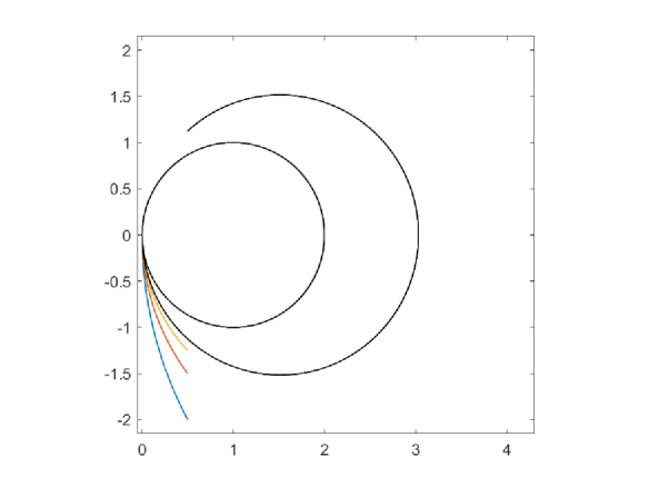
Figure 6: Trajectories of symplectic Euler discretisation for different initial conditions.

Figure 6 illustrates trajectories of (4.1) corresponding to four initial conditions $(x_{0},\,y_{0})$ satisfying $(x_{0}-1)^{2}+y_{0}^{2}>1$, when $h=10^{-4}$. In all cases, the numerical trajectories traverse the level sets of $H$ to high accuracy. Near the origin $(0,\,0)$, the trajectories switch to the unit circle $(x-1)^{2}+y^{2}=1$ as expected from the entropy rate admissibility criterion. The black trajectory, which corresponds to the initial condition $(x_{0},\,y_{0})=(\frac{1}{2},\,\frac{9}{8})$, is further analysed below.

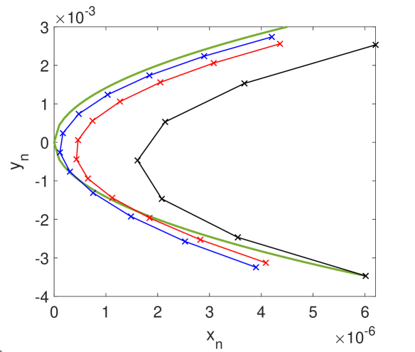
Figure 7: Trajectories for symplectic Euler discretisation near $(0,\,0)$ for $h=2.5\times 10^{-4}$(blue); $h=5\times 10^{-4}$(red); $h=10^{-3}$(black). The unit circle $(x-1)^{2}+y^{2}=1$ in green.

Figure 7 shows the behaviour near the origin in varying detail depending upon step size: $h=2.5\times 10^{-4}$(blue), $h=5\times 10^{-4}$(red), $h=10^{-3}$(black). All trajectories start from the same initial condition $(x_{0},\,y_{0})$, cross the $x-$axis at a positive value $x\sim h^{2}$ and then follow the unique solution close to the unit circle. The well-known analysis of the symplectic Euler method of the linear equation in the domain $(x-1)+y^{2}<1$ shows that the trajectory remains in a neighbourhood of the unit circle of order $h$. The rigorous analysis presented in [13, Chapt. 11], however, is required to establish that trajectories always cross the $x-$axis at points $x>0,$ and thereafter enter and remain near the unit circle. In fact, for small $h$, the level sets of $H$ are perturbed to the right near the origin. The geometry of the discrete flow explains the selection of the solution obtained by the entropy rate admissibility criterion.

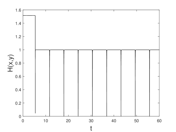
Figure 8: $H(x,y)$ as function of $t$ for initial condition $(x_{0},\,y_{0})=(\frac{1}{2},\frac{9}{8})$.

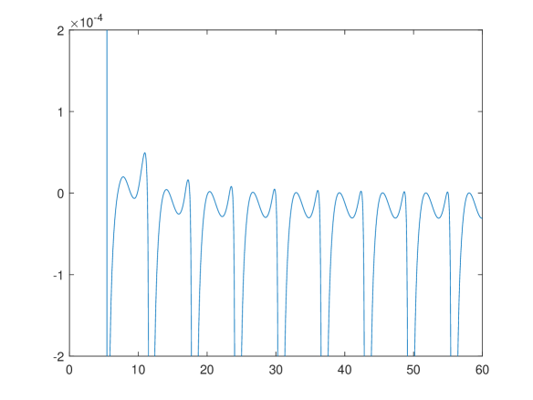
Figure 9: Error $(H(x,y)-1)$ as function of $t$ for initial condition $(x_{0},\,y_{0})=(\frac{1}{2},\,\frac{9}{8}).$

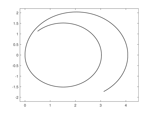
Figure 10: Trajectory of explicit Euler discretisation for initial condition $(x_{0},\,y_{0})=(\frac{1}{2},\,\frac{9}{8}).$

Figure 8 depicts the numerically computed entropy profile $t\mapsto H(x(t),\,y(t))$ for initial condition $(x_{0},\,y_{0})=(\frac{1}{2},\,\frac{9}{8})$ introduced above. Again take $h=10^{-4}$. When the trajectory first passes through the origin, $H$ drops to a value near $1$ and then remains approximately constant.

Figure 9 indicates the discretisation error in the entropy profile $t\mapsto\left[H(x(t),\,y(t))-1\right].$ The error is of size less than $10^{-4}=O(h)$ except for floating point errors when $(x,\,y)$ is near the origin where $H$ possesses a singularity.

It has thus been shown how geometric properties in phase space of the symplectic Euler method select the solution to the system (2.29) and (2.30) according to the entropy rate admissibility criterion. Numerical methods without such properties are not expected to select these solutions.

Figure 10 shows the trajectory computed by the explicit Euler method again for initial condition $(x_{0},\,y_{0})=(\frac{1}{2},\,\frac{9}{8})$. For this discretisation, the numerical solution moves to a larger circle with increased entropy $H$, even with smaller step size $h=10^{-5}.$

5 Relevant convex integration results

Section 2 describes how the entropy rate admissibility criterion applied to the constant functions (2.6) selects a unique orbit from the infinitely many circular paths generated by the Dafermos equations (2.1) and (2.2). A piecewise non-increasing linear graph of maximal negative slope leads to the requisite single profile. A notable feature of the construction, stated in Theorem 2.1, is the uncountable number of profiles that can be arbitrarily chosen for prescribed initial conditions.

This feature resembles results of Buckmaster and Vicol [4] and of De Lellis and Szèkelyhidi [10] which for convenience are recalled in the following theorem.

Theorem 5.1.

There exists $\beta>0$ such that for any non-negative smooth function $E(t):[0,T]\rightarrow\mathrm{I\!R\!}_{\geq 0}$ there exists a weak vector solution $\textbf{v}\in C^{0}_{t}\left([0,T];H^{\beta}_{x}(\mathrm{I\!T\!}^{3})\right)$ of the Navier-Stokes equations such that

$$\int_{\mathrm{I\!T\!}^{3}}|\textbf{v}(x,t)|^{2}\,dx=E(t),$$

for all $t\in[0,T]$. Moreover, the associated vorticity $\nabla\times\textbf{v}$ lies in $C^{0}_{t}\left([0,T];L^{1}_{x}(\mathrm{I\!T\!}^{3})\right),$ where $\mathrm{I\!T\!}^{3}=\mathrm{I\!R\!}^{3}\backslash 2\pi Z^{3}$ denotes the unit cube with periodic boundary conditions.

It is apparent that arbitrary prescription of the energy $E(t)$ produces an infinite number of solutions in the given class for the same initial conditions. An admissibility criterion is required to identify a single physically relevant velocity. Whether an entropy rate admissibility criterion of the type considered here is appropriate in this respect remains an important open question.

A detailed comparison with the analysis of Section 3 reveals distinct differences and any analogy between the two treatments is likely to be superficial. Indeed, the entropy $H(x,\,y)$ used in Section 3 is not a local (kinetic) energy function $\eta(t)$ defined by

$$\eta(t):=\frac{\rho}{2}\left(\dot{x}^{2}+\dot{y}^{2}\right)$$ (5.1)

where $\rho(x,y)$ is a specified density. The relation to $H(x,y)$ is obtained by substitution of (2.10) and (2.11) in (5.1) and is given by

$$\eta(t)=2x^{2}w^{2}(x,y)\rho(x,y)H^{2}(x,y).$$ (5.2)

Consequently, functions $\eta$ and $H^{2}$ are identical only when $2x^{2}w^{2}\rho=1$.

Finally, note that uniqueness properties arising in convex integration studies refer to solutions of the respective equations and not to the associated Lagrange trajectories. Whether there are non-unique trajectories for certain non-unique convex integration solutions remains a second open question.

Acknowledgements:

Valuable discussions during the preparation of this paper with Professors Z. Artstein, E. Feireisl, A. Ostermann and E. Titi are gratefully acknowledged. Topics treated in this paper first arose during the 2021 Workshop on Convex Integration and Partial Differential Equations organised by ICMS, Edinburgh.

Appendices

Appendix A State variables.

Let state variables $(x(t),\,y(t))$ satisfy (2.1) and (2.2) in region $\Omega_{1}$ defined by (2.35). Consider for $x\neq 0,\,y\neq 0,$ the expression

$$\frac{d}{dt}\left(\frac{y^{2}}{x}\right) = \frac{y}{x^{2}}\left(2\dot{y}x-y\dot{x}\right)$$

$$= \frac{y}{x^{2}}\left(y^{2}-x^{2}-y\dot{x}\right)$$

$$= \frac{y}{x^{2}}\left(y\dot{x}-x^{2}-y\dot{x}\right)$$

$$= -y$$

$$= -\dot{x},$$

which on integration gives (cp., (2.20))

$$\frac{y^{2}}{x}+x=\frac{y^{2}_{0}}{x_{0}}+x_{0}\equiv 2c_{0}$$ (A.1)

or

$$(x-c_{0})^{2}+y^{2}=c_{0}^{2},$$

which may be rewritten as

$$y(t)=\pm\sqrt{x(2d-x)}\qquad(=\dot{x}).$$

On setting $c_{0}z(t)=(x(t)-c_{0})$ the last expression becomes

$$\dot{z}(t)=\pm\sqrt{(1-z^{2})},$$

so that

$$z(t)=\pm\cos{(\mp t+\sin^{-1}{z_{0}})},$$

and therefore

$$x(t)=c_{0}\pm c_{0}\cos{(\mp t+\sin^{-1}{z_{0}})}.$$ (A.2)

A corresponding expression for $y(t)$ obtained on differentiation of the last relation is

$$y(t)=\pm c_{0}\sin{(\mp t+\sin^{-1}{z_{0}})}.$$ (A.3)

The positive root in (A.2) and (A.3) yields (2.21) and (2.22) with $\theta_{0}=\sin^{-1}{z_{0}}$ given by (cp., (2.23))

$$\tan{\theta_{0}}=\frac{y_{0}}{(x_{0}-c_{0})}.$$

Alternatively, elimination of the dependent variable $y$ between (2.1) and (2.9) leads to a differential equation for $x$ whose solution is

$$x(t)-c_{0}=A\cos{(t)}+B\sin{(t)},$$ (A.4)

and consequently

$$y(t)=-A\sin{(t)}+B\cos{(t)},$$ (A.5)

where $A,\,B,$ constants determined by initial conditions $(x_{0},\,y_{0})$, are given by

$$A = x_{0}-c_{0},$$ (A.6)

$$B = y_{0},$$ (A.7)

and $c_{0}$ is specified by (A.1). Expressions (A.4) and (A.5) are equivalent to (A.2) and (A.3).

Appendix B Navier-Stokes equations.

Throughout Appendix B and Appendix C a suffix notation and summation convention are adopted together with a subscript comma to denote partial differentiation. Components of vectors, unless otherwise stated, are with respect to a given Cartesian coordinate system.

Consider a compressible fluid (of variable density) in plane steady motion that satisfies the isotropic Navier-Stokes equation for a given velocity field having Cartesian components $(v_{1},\,v_{2})$. The aim, using a semi-inverse method, is to determine the viscosity coefficients $\lambda(x_{1},\,x_{2})$ and $\mu(x_{1},\,x_{2})$ that ensure the corresponding stress distribution is in equilibrium subject to zero body force. The region occupied by the fluid is not defined at this stage. Nor are boundary conditions considered.

The compatible strain rate components, given by

$$e_{\alpha\beta}=\frac{1}{2}\left(v_{\alpha,\beta}+v_{\beta,\alpha}\right),\qquad\alpha,\,\beta=1,2,$$ (B.1)

are related to the stress components by (3.25)-(3.27) concisely written as

$$\sigma_{\alpha\beta}=\lambda e_{\gamma\gamma}\delta_{\alpha\beta}+2\mu e_{\alpha\beta},$$ (B.2)

where $\delta_{\alpha\beta}$ denotes the Kronecker delta. The viscosity coefficients $\lambda(x_{1},\,x_{2}),\,\mu(x_{1},\,x_{2})$ are functions of position to be determined such that the stress is in equilibrium under zero body force; that is

$$\sigma_{\alpha\beta,\beta}=0.$$ (B.3)

In consequence, the Navier-Stokes equations (3.25) and (3.26) reduce to the Euler equations (3.10) and (3.11).

Easy deductions from (B.2) are the trace relation

$$\sigma_{\alpha\alpha}=2(\lambda+\mu)e_{\alpha\alpha},$$ (B.4)

and

$$2\mu=\frac{\left(\sigma_{11}-\sigma_{22}\right)}{\left(e_{11}-e_{22}\right)}=\frac{\sigma_{12}}{e_{12}},$$ (B.5)

which represents an additional fundamental constraint between stress and strain rate explicitly independent of viscosity coefficients. Trivial rearrangement of (B.5) gives

$$\frac{\left(\sigma_{11}-\sigma_{22}\right)}{\sigma_{12}}=\frac{\left(e_{11}-e_{22}\right)}{e_{12}}.$$ (B.6)

It is well-known that a solution to the system (B.3) expressed in terms of the Airy stress function $\chi(x,y)$ is represented by:

$$\sigma_{11}=-\chi_{,22},\qquad\sigma_{22}=-\chi_{,11},\qquad\sigma_{12}=\chi_{,12}.$$ (B.7)

Substitution of (B.7) in (B.6) yields

$$\chi_{,11}-\chi_{,22}-\Lambda(x_{1},\,x_{2})\chi_{,12}=0,\qquad\Lambda:=\frac{(e_{11}-e_{22})}{e_{12}},$$ (B.8)

which is the partial differential equation satisfied by the Airy stress function $\chi(x,y)$ explicitly independent of viscosity coefficients $\lambda,\,\mu$.

On the assumption that (B.8) can be solved for general $(v_{1},\,v_{2})$ and therefore $\Lambda$, the solution may be used to derive the equilibrium stress components and consequently the viscosity coefficient $\mu$ from (B.5)₃. Furthermore, it follows from (B.7) and (B.4) that

$$\chi_{,\alpha\alpha}=-2(\lambda+\mu)(e_{11}+e_{22}),$$ (B.9)

which may be used to determine $(\lambda+\mu)$ and therefore $\lambda(x_{1},x_{2})$.

Appendix C Derivation of viscosity coefficients in Theorem 3.2

Derivation of expressions (3.20) and (3.21) for the viscosity coefficients stipulated in Theorem 3.2 is conveniently described in terms of the complex variable $z$ and its conjugate $\bar{z}$ defined by

$$z=(x_{1}+ix_{2}),\qquad\bar{z}=(x_{1}-ix_{2}).$$ (C.1)

Details of the following computations are contained in standard texts; e.g., Muskhelishvili [17].

Differentiation with respect to $z$ and $\bar{z}$ is defined to be

$$\frac{\partial}{\partial z} := \frac{1}{2}\left(\frac{\partial}{\partial x}-i\frac{\partial}{\partial y}\right),$$ (C.2)

$$\frac{\partial}{\partial\bar{z}} := \frac{1}{2}\left(\frac{\partial}{\partial x}+i\frac{\partial}{\partial y}\right).$$ (C.3)

The particular velocity components (2.1) and (2.2) of present concern, repeated for convenience

$$v_{1}=x_{2},\qquad v_{2}=\frac{(x^{2}_{2}-x_{1}^{2})}{2x_{1}},\qquad(x_{1},\,x_{2})\in\Omega_{1},$$ (C.4)

are the real and imaginary parts of the (non-analytic) velocity field $v(z,\,\bar{z})$ represented by

$$v=v_{1}+iv_{2}=-i\frac{z^{2}}{\left(z+\bar{z}\right)}.$$ (C.5)

The corresponding strain rate components become

$$e_{11} = 0,$$ (C.6)

$$e_{22} = i\frac{\left(\bar{z}-z\right)}{\left(z+\bar{z}\right)},$$ (C.7)

$$e_{12} = \frac{1}{2}\frac{\left(z^{2}+\bar{z}^{2}\right)}{\left(z+\bar{z}\right)^{2}}.$$ (C.8)

Insertion into the formula for $\Lambda(z,\bar{z})$ (see (B.8)₂) gives

$$\Lambda=2i\frac{\left(z^{2}-\bar{z}^{2}\right)}{\left(z^{2}+\bar{z}^{2}\right)}.$$ (C.9)

Consequently, (B.8) assumes the form

$$\left(\chi_{,zz}+\chi_{,\bar{z}\bar{z}}\right)\left(z^{2}+\bar{z}^{2}\right)+\left(\chi_{,zz}-\chi_{,\bar{z}\bar{z}}\right)\left(z^{2}-\bar{z}^{2}\right)=0,$$ (C.10)

which upon rearrangement simplifies to

$$z^{2}\chi_{,zz}+\bar{z}^{2}\chi_{,\bar{z}\bar{z}}=0.$$ (C.11)

Among the possible solutions to (C.11), select that obtained from setting

$$z^{2}\chi_{,zz}=k=-\bar{z}^{2}\chi_{,\bar{z}\bar{z}},$$ (C.12)

for real constant $k$. Integration of the equation on the left gives

$$\chi(z,\bar{z})=-k\log{z}+zf(\bar{z})+q(\bar{z}),$$ (C.13)

where $f(.),\,q(.)$ are arbitrary functions. Similarly, integration of the equation on the right of (C.12) yields

$$\chi(z,\bar{z})=k\log{\bar{z}}+\bar{z}g(z)+p(z),$$ (C.14)

where $g(.),\,p(.)$ are arbitrary functions. Choose

$$p(z) = -k\log{z},\qquad q(\bar{z})=k\log{\bar{z}},$$

$$g(z) = 2z\log{z},\qquad f(\bar{z})=-2\bar{z}\log{\bar{z}}.$$

to derive respectively from (C.13) and (C.14) the equivalent expressions

$$\chi(z,\bar{z}) = -k\log{\frac{z}{\bar{z}}}-2z\bar{z}\log{\bar{z}},$$

$$\chi(z,\bar{z}) = -k\log{\frac{z}{\bar{z}}}+2z\bar{z}\log{z},$$

and consequently the final form for the Airy stress function $\chi(z,\bar{z})$ is:

$$\chi(z,\bar{z})=\left(z\bar{z}-k\right)\log{\frac{z}{\bar{z}}}.$$ (C.15)

Substitution in (B.7) determines the equilibrium stress components as

$$\sigma_{11}(z,\bar{z}) = i\left[(z\bar{z}+k)\frac{(z^{2}-\bar{z}^{2})}{(z\bar{z})^{2}}+2\log{\frac{z}{\bar{z}}}\right],$$ (C.16)

$$\sigma_{22}(z,\bar{z}) = i\left[(z\bar{z}+k)\frac{(\bar{z}^{2}-z^{2})}{(z\bar{z})^{2}}+2\log{\frac{z}{\bar{z}}}\right],$$ (C.17)

$$\sigma_{12}(z,\bar{z}) = \frac{(z\bar{z}+k)(z^{2}+\bar{z}^{2})}{(z\bar{z})^{2}},$$ (C.18)

while the viscosity coefficient $\mu(z,\,\bar{z})$ from (B.5)₃ and (C.8) is given by

$$\mu=\frac{(z\bar{z}+k)(z+\bar{z})^{2}}{(z\bar{z})^{2}}.$$ (C.19)

In view of (C.6), (C.6),(C.7) and (C.16), the viscosity coefficient $\lambda(z,\,\bar{z})$ is

$$\lambda = \frac{\sigma_{11}}{e_{22}}$$

$$= \frac{2(z+\bar{z})}{(\bar{z}-z)}\log{\frac{z}{\bar{z}}}-\frac{(z\bar{z}+k)(z+\bar{z})^{2}}{(z\bar{z})^{2}}.$$

In terms of polar coordinates $(r,\theta)$, where

$$z=r\exp{(i\theta)},\qquad\bar{z}=r\exp{(-i\theta)},$$

these expressions are written as

$$\sigma_{11} = -2\left[2\theta+\left(\frac{(r^{2}+k)}{r^{2}}\sin{2\theta}\right)\right],$$

$$\sigma_{22} = 2\left[-2\theta+\left(\frac{(r^{2}+k)}{r^{2}}\sin{2\theta}\right)\right],$$

$$\sigma_{12} = 2\left(\frac{(r^{2}+k)}{r^{2}}\right)\cos{2\theta},$$

$$e_{11} = 0,$$

$$e_{22} = \tan{\theta},$$

$$e_{12} = \frac{\cos{2\theta}}{4\cos^{2}{\theta}},$$

$$\mu = 4\frac{(r^{2}+k)}{r^{2}}\cos^{2}{\theta},$$

$$\lambda = -4\theta\cot{\theta}-4\left(\frac{(r^{2}+k)}{r^{2}}\right)\cos^{2}{\theta}.$$

It may easily be checked by direct substitution that the stress is in equilibrium under zero body force and that

$$v_{\alpha}n_{\alpha}=0$$

at all points on $\partial\Omega_{1}\backslash(0,0)$.

The proof of (3.20) and (3.21) is complete on taking $k=0$ in the above expressions.

Appendix D Conservative Lagrange trajectories

Let $(x,y)$ be the rectangular coordinates of a point moving with respect to time and suppose that the differentiable function $G(x,y)$ is conserved so that $G(x(t),\,y(t))$ is constant. Examples are the entropy in an adiabatic system or a one parameter family of plane closed curves discussed in Section 2. Define velocities $(u,\,v)$ by

$$u(x,t) := \dot{x},$$ (D.1)

$$v(x,t) := \dot{y},$$ (D.2)

to obtain from

$$\frac{dG(x(t),\,y(t))}{dt}=0$$

the relation

$$\frac{\partial G}{\partial x}u+\frac{\partial G}{\partial y}v=0.$$ (D.3)

Consequently, any $u$ determines $v$ from the expression

$$v=-\frac{\partial G}{\partial x}\left(\frac{\partial G}{\partial y}\right)^{-1}u$$ (D.4)

such that the system (D.1) and (D.2) is conservative with $G(x,y)$ as first integral.

The particular choice

$$u(x,y)=\frac{\partial G}{\partial y}$$ (D.5)

yields a Hamiltonian system for which

$$v=-\frac{\partial G}{\partial x}.$$ (D.6)

It follows that the incompressibity condition

$$\frac{\partial u}{\partial x}+\frac{\partial v}{\partial y}=0$$ (D.7)

holds provided the order of the second partial derivatives of $G$ can be reversed.

For fluids with variable mass density, the continuity equation is satisfied by modifying the definition of $u$. Thus, suppose

$$u:=\frac{\partial G}{\partial y}w(x,\,y),$$ (D.8)

where $w(x,\,y)$ is some sufficiently smooth function, and $G(x,\,y)$ continues to be the first integral of the conservative system (D.1) and (D.2). Accordingly, $v(x,\,y)$ is modified to

$$v:=-\frac{\partial G}{\partial x}w(x,\,y),$$ (D.9)

and the continuity equation

$$\frac{\partial}{\partial x}(\rho u)+\frac{\partial}{\partial y}(\rho v)=0,$$ (D.10)

is satisfied provided when $(i)$ the mass density $\rho(x,y)$ is chosen to be $\rho=Dw^{-1}$, for constant $D$, and $(ii)$ the order of the second partial derivatives of $G$ can be reversed.

Remark D.1.

Apart from differentiability of $G$, no further assumptions have been introduced on either $G(x,\,y)$ or $w(x,\,y)$, whose choice clearly determines the smoothness of the mass density $\rho(x,\,y)$.

Remark D.2.

Lagrange trajectories corresponding to the system (3.1) and (3.2) are a special case of (D.1) and (D.2) upon selecting $w(x,y)=x$ and setting

$$G(x,\,y)=\frac{(x^{2}+y^{2})}{2x}\quad\left(=H(x,y)\right).$$ (D.11)

The mass density becomes $\rho=x^{-1}$ and

$$\frac{\partial G}{\partial x}=\frac{(x^{2}-y^{2})}{2x^{2}},\qquad\frac{\partial G}{\partial y}=\frac{y}{x}.$$ (D.12)

which on insertion into (D.8) and (D.9) yields the required velocity components. Note that

$$\frac{\partial^{2}G}{\partial x\partial y}\neq\frac{\partial^{2}G}{\partial y\partial x}\qquad\mbox{ for }(x,\,y)=(0,\,0).$$

Remark D.3.

Substitution of (D.8) and (D.9) in the Euler equations yields equations for the partial derivatives of the pressure which can be solved for the pressure. Consequently, for any conserved quantity $G(x,y)$ and any choice of $w(x,\,y)$ the Euler equations can be solved for appropriate pressure determined semi-inversely.

When $w=x$ the pressure is given by (3.12) which to within a constant is the conserved quantity $G(x,y)$ given by (D.11).

Remark D.4.

For the choice $w(x,\,y)=x^{\alpha},\,0<\alpha<1$, the density becomes $\rho=x^{-\alpha}$ and though singular at the origin, is integrable on the region $\Omega$ and computations involving mass density are valid.

References

- [1] Artstein, Z. (1983). Stabilization with relaxed controls. Nonlinear Analysis, 7, 1163-1173.
- [2] Breit, D., Feireisl, E. and Hofmanova, M. (2020). Dissipative solutions and semi-flow selection for the complete Euler system. Commun. Math. Phys., 376(2), 1471-1497.
- [3] Brenier, Y. (2018). The initial value problem for the Euler equations of incompressible fluids viewed as a concave maximization problem. Commun. Math. Phys., 365, 579-605.
- [4] Buckmaster, T. and Vicol, V. (2019). Nonuniqueness of weak solutions to the Navier-Stokes equation. Ann. of Math., 189, 101-144.
- [5] Burkill, J. C. (1975). The Theory of Ordinary Differential Equations. Third Edition. Longman Group. London New York.
- [6] Chiodaroli, E. and Kreml, O. (2014). On the energy dissipation rate of solutions to the compressible isentropic Euler system. Arch. Rational Mech. Anal., 214, 1019-1049.
- [7] Dafermos, C. M. (2012). Maximal dissipation in equations of evolution. J. Diff. Eqns., 252, 567-587.
- [8] De Lellis, C. and Szèkelyhidi, L. (2009). The Euler equations as a differential inclusion. Ann. of Math., 170(3), 1417-1436.
- [9] De Lellis, C. and Szèkelyhidi, L. (2010). On admissibility criteria for weak solutions of the Euler equations. Arch. Rational Mech. Anal., 195(1), 225-260.
- [10] De Lellis, C. and Szèkelyhidi, L. (2013). Dissipative continuous Euler flows. Invent. Math., 193, 377-407.
- [11] Feireisl, E. (2014). Maximal dissipation and well-posedness for the compressible Euler system. J. Math. Fluid Mech., 16, 447-461.
- [12] Glimm, J., Lazarev, D. and Chen, G.-Q. G. (2020). Maximum entropy production as a necessary admissibility condition for the fluid Navier-Stokes and Euler equations. SN Applied Sciences, 2, 2160.
- [13] Hairer, E., Lubich, C. and Wanner, G. (2006). Geometric Numerical Integration. Second Edition. Springer Series in Computational Mathematics 31. Springer-Verlag. Berlin Heidelberg.
- [14] Lasarzik, R. (2022). Maximally dissipative solutions for incompressible fluid dynamics. Z. Angew. Math. Phys., 73, 1-21.
- [15] Lions, P.-L. (1996). Mathematical Topics in Fluid Mechanics. Vol. I. The Clarendon Press. Oxford New York.
- [16] Moroz, A. (2011). The Common Extremalities in Biology and Physics. Elsevier Insights. Elsevier.
- [17] Muskhelishvili, N. I. (1963). Some Basic Problems of the Mathematical Theory of Elasticity. 4th Edition. Translated by J. R. M. Radok. Groningen. Noordhoff.
- [18] Prigogine, I. (1947). Étude Thermodynamique des Phenomenes Irreversibiles. Editions Desoer. Liege.
- [19] Robinson, J. C. and Sadowski, W. (2009). Almost-everywhere uniqueness of Lagrangian trajectories for suitable weak solutions of the three-dimensional Navier-Stokes equations. Nonlinearity, 22, 2093-2099.
- [20] Robinson, J. C. and Sadowski, W. (2009). A criterion for uniqueness of Langrangian trajectories for weak solutions of the 3D Navier-Stokes equations. Commun. Math. Phys., 290, 15-22.
- [21] Scheffer, V. (1993). An inviscid flow with compact support in space-time. J. Geom. Anal., 3, 343-401.
- [22] Shnirelman, A. (1997). On the nonuniqueness of weak solutions of the Euler equation. Comm. Pure Appl. Math., 50, 1261-1286.
- [23] Ziegler, H. (1983). Chemical reactions and the principle of maximal rate of entropy production. Z. Angew. Math. Phys., 34, 832-844.