Synchrotron emission from double-peaked radio light curves of the symbiotic recurrent nova V3890 Sagitarii

Abstract

We present radio observations of the symbiotic recurrent nova V3890 Sagitarii following the $2019$ August eruption obtained with the MeerKAT radio telescope at $1.28$ GHz and Karl G. Janksy Very Large Array (VLA) at $1.26~{}-35$ GHz. The radio light curves span from day $1$ to $540$ days after eruption and are dominated by synchrotron emission produced by the expanding nova ejecta interacting with the dense wind from an evolved companion in the binary system. The radio emission is detected early on (day $6$) and increases rapidly to a peak on day $15$. The radio luminosity increases due to a decrease in the opacity of the circumstellar material in front of the shocked material and fades as the density of the surrounding medium decreases and the velocity of the shock decelerates. Modelling the light curve provides an estimated mass-loss rate of ${\overset{\hbox{\tiny$\bullet$}}{M}}_{\textrm{wind}}\approx 10^{-8}{\textrm{M}}_{\odot}~{}{\textrm{yr}}^{-1}$ from the red giant star and ejecta mass in the range of $M_{\textrm{ej}}=10^{-5}-10^{-6}~{}{\textrm{M}}_{\odot}$ from the surface of the white dwarf. V3890 Sgr likely hosts a massive white dwarf similar to other symbiotic recurrent novae, thus considered a candidate for supernovae type Ia (SNe Ia) progenitor. However, its radio flux densities compared to upper limits for SNe Ia have ruled it out as a progenitor for SN 2011fe.

1 Introduction

V3890 Sgr belongs to a class of cataclysmic variables known as symbiotic recurrent novae; “symbiotic" because the accreting white dwarf has a giant companion (e.g., Schaefer, 2010). It is a recurrent nova because more than one thermonuclear eruption has been observed from this system; the most recent eruption occurred on $2019$ August $27.9$ UT as reported by A. Pereira (Strader et al., 2019; Kafka, 2020). Previous eruptions of the nova were observed in $1962$ June (Wenzel, 1990; Miller, 1991) and $1990$ April $27.7$ (e.g., Buckley et al., 1990; Anupama & Sethi, 1994).

Initially, the orbital period of V3890 Sgr was estimated as $519.7$ days (Schaefer, 2009). However, recently using optical observations, Mikołajewska et al. (2021) estimated an orbital period of $747.6$ days for V3890 Sgr. The nova is therefore, in the same class as other long period recurrent novae such as RS Oph, V745 Sco, T CrB and V2487 Oph (Anupama & Mikołajewska, 1999; Schaefer, 2009, 2010). Since some of the symbiotic recurrent novae have been extensively studied, their known parameters are listed in Table 1 and compared with V3890 Sgr.

The optical light curves of these recurrent symbiotic novae evolve quickly following an eruption due to the low mass of material accreted onto the surface of the white dwarf since the last nova eruption, as these systems are known to host massive white dwarfs ($\gtrsim 1.2~{}\textrm{M}_{\odot}$; see Table 1). The ejecta outflows following an eruption are also fast, with velocities $\gtrsim 4000~{}\textrm{km~{}s}^{-1}$ measured from emission lines observed during different stages of the spectral evolution (see Table 1). The emission lines, however, become narrower with time during the early phase of the ejecta evolution, as the nova ejecta sweep up and are decelerated by the wind from the secondary star (e.g., Gonzalez-Riestra, 1992; Banerjee et al., 2014; Mondal et al., 2018).

Table 1: Estimated parameters of the symbiotic recurrent novae based on multiwavelength studies of individual systems. Listed parameters include masses of the binary components, the spectral classification of the companion star, orbital period ($P_{\textrm{orbit}}$), years of recorded eruptions, the nova recurrence time ($t_{\textrm{rec}}$), velocity of the ejected material ($V_{\textrm{ej}}$), the time it takes for the nova to fade from optical maximum by $3$ magnitudes ($t_{3}$), and the distance to the nova ($d$).

Name	$M_{\textrm{white dwarf}}$	$M_{\textrm{giant}}$	Spectral	$P_{\textrm{orbit}}$	years of	$t_{\textrm{rec}}$	$V_{\textrm{ej}}$	$t_{3}$	$d$
	M⊙	M⊙	type	(days)	eruption	(yrs)	($\textrm{km~{}s}^{-1})$	(days)	(kpc)
T CrB	1.37 (1)	1.12 (1)	M4 III (2)	228 (3)	1866, 1946	80		6 (8)	0.81 (4)
RS Oph	1.2 –	0.7–	M0–2 III (6)	453.6 (5)	1898, 1907, 1933, 1945	$\gtrsim 10$	4200 (7)	14 (8)	1.6 (9)
	1.4 (5)	0.8 (5)			1958, 1967, 1985, 2006, 2021
V745 Sco			M4 III (10)	510 (8)	1937, 1963, 1989, 2014	25	> 4000 (11)	9 (8)	7.8 (8)
V3890 Sgr	1.35 (12)	1.1 (12)	M5 III (10)	747.6 (12)	1962, 1990, 2019	28	$\gtrsim 4200$ (13)	14 (8)	9 (12)

• References: (1) Stanishev et al., 2004; (2) Mürset & Schmid, 1999; (3) Kenyon & Garcia, 1986; (4) Bailer-Jones et al., 2018; (5) Brandi et al., 2009; (6) Anupama & Mikołajewska, 1999; (7) Mondal et al., 2018; (8) Schaefer, 2010; (9) Hjellming et al., 1986; (10) Harrison et al., 1993; (11) Banerjee et al., 2014; (12) Mikołajewska et al., 2021; (13) Strader et al., 2019; (14) Munari & Walter, 2019b

Recurrent novae have short recurrence times of less than a century (see Table 1), which are attributed to high accretion rates, $\dot{M}\approx 10^{-8}~{}\textrm{M}_{\odot}~{}\textrm{ yr}^{-1}$ (Yaron et al., 2005). The high rates rapidly supply enough material to power the subsequent thermonuclear runaway. Theoretically, most recurrent novae also consist of massive white dwarfs, and therefore require less mass to accumulate for hydrogen ignition (e.g., Prialnik & Kovetz, 1995; Yaron et al., 2005; Wolf et al., 2013). In symbiotic systems, the high $\dot{M}$ is acquired through mass loss from the companion red giant, which is accreted either as a wind or through a disc via the inner Lagrangian point (Luna, 2019). The mass loss via the giant’s wind also contributes to a dense circumstellar environment, which is impacted by the expanding nova envelope to give rise to shocks observed at high energies such as X-rays (e.g., Bode & Kahn, 1985; Sokoloski et al., 2006) and $\gamma-$rays (Zheng et al., 2022).

A combination of high-mass white dwarfs and high mass accretion rates make the eruptions of these systems relatively gentle, and consequently not all of the accreted material is ejected during eruption (Yaron et al., 2005). The white dwarf may therefore grow in mass towards the Chandrasekhar limit. Indeed, the white dwarfs in recurrent novae have been shown to be massive (Osborne et al., 2011; Page et al., 2015), and these systems have therefore been proposed as progenitors of supernovae type Ia Maoz et al. (2014). However, it is not clear whether the underlying white dwarfs in recurrent symbiotic novae are composed of CO or ONe. A CO white dwarf is required for a SN Ia; the fate of an ONe white dwarf that has grown in mass towards the Chandrasekhar limit is instead an accretion-induced collapse into a neutron star (Gutierrez et al., 1996).

Based on previous eruptions, the optical evolution of V3890 Sgr is fast, taking less than a day to rise to maximum magnitude ($V\approx~{}8$ mag) and $14$ days for the brightness to drop by $3$ mag; it is therefore classified as a fast nova (Payne-Gaposchkin, 1964; Schaefer, 2010).

The spectral evolution of V3890 Sgr at ultraviolet wavelengths shows the presence of both broad and narrow emission lines (Gonzalez-Riestra, 1992). The broad lines originate from the expanding nova ejecta, while the narrow lines represent the speed of the red giant wind (e.g., Munari, 2019). The FWHMs of the hydrogen Balmer lines decrease with time, from $2140~{}\textrm{km~{}s}^{-1}$ to $210~{}\textrm{km~{}s}^{-1}$ within a period of $13$ days following the eruption in 1990 (Gonzalez-Riestra, 1992). Following the $2019$ eruption, the nova was observed with the Gemini observatory to obtain near-infrared spectra during the early days after the outburst (Evans et al., 2022). During this time, Helium emission lines showed both broad and narrow components. The broad lines emerged on day $3$ and narrowed through day $23$ (Evans et al., 2022). This is interpreted as evidence of the high velocity nova envelope being decelerated with time as it sweeps up the red giant wind.

The rise, peak and decay of the optical light curve of V3890 Sgr following the $2019$ August eruption is well observed (Strader et al., 2019; Sokolovsky et al., 2019). The optical evolution of the nova shown in Figure 1 is similar to previous outbursts (see Figure 1).

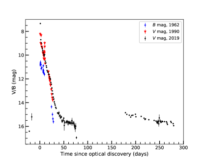
Figure 1: The $V$-band and $B$-band optical light curves of the $1962$, $1990$ and $2019$ eruptions of V3890 Sgr from AAVSO data (Kafka, 2020) and data presented by Schaefer (2010). Here we set $t_{0}$ to time of the eruptions (Sokolovsky et al., 2019).

The eruption has been observed at $\gamma-$ray, X-ray, infrared, UV, optical, and radio wavelengths (Buson et al., 2019; Orio et al., 2020; Ness et al., 2022; Kaminsky et al., 2022; Evans et al., 2022; Nyamai et al., 2019; Polisensky et al., 2019). V3890 Sgr was detected in $\gamma$-rays and hard X-rays very soon ($\sim 2$ days) following the eruption (Buson et al., 2019; Sokolovsky et al., 2019), consistent with expectations for a nova erupting in a dense environment.

Presented in this paper are radio observations of V3890 Sgr with MeerKAT at $1.28$ GHz and the VLA at radio frequencies between 1.26 GHz to $35$ GHz. The observations are used to study the transient phenomena of the system at radio frequencies. In §2, radio observations and measurements including the radio light curve, radio spectral evolution and H i absorption analysis are presented. The emission from the nova, modelled as synchrotron radiation emanating from the interaction of the ejecta with the red giant wind, is analyzed in §3. The conclusions are highlighted in §4.

2 Radio observations

2.1 MeerKAT and VLA observations of V3890 Sgr

Monitoring of V3890 Sgr with the MeerKAT telescope started on ($t-t_{0})\approx 2$ days, where $t_{0}$ is taken as $2019$ August $27.9$ (MJD 58722.9). V3890 Sgr is the first recurrent nova to be studied with MeerKAT. MeerKAT is a radio telescope located in South Africa and consists of $64$ dishes each with a diameter of $13.5$ m (Jonas & MeerKAT Team, 2016). Combined, they form an array with a maximum baseline of $8$ km. The observations were taken using the MeerKAT L-band receiver, which has a total bandwidth of $856$ MHz split into $4096$ channels each with a width of $209$ kHz. The frequency range covered is $0.9$ to $1.67$ GHz centred at $1.284$ GHz. In each observation, the time on target was between $15$ and $30$ minutes (see Table 2). For the first $15$ days after optical discovery, V3890 Sgr was observed daily and then every two days afterwards until day $25$. Later, the observations were carried out once every week and finally the cadence was slowed down further to twice every month until the end of the observations on $2020$ May $26$. For all the epochs, the flux and bandpass calibrator J1939-6342 was observed for $\thicksim 5$ mins. The complex gain (secondary) calibrator J1911-2006 was observed for $2$ minutes per visit before and after observing the target.

V3890 Sgr was observed with the VLA from $2019$ Aug $30$ to $2021$ Feb $13$ at observing frequencies between $1$ GHz and $37$ GHz. Observations were conducted using the L, C, Ku, and Ka band receivers. The total bandwidth was $1$ GHz for L band ($1-2$ GHz), $4$ GHz for C band ($4-8$ GHz), $6$ GHz for Ku band ($12-18$ GHz), and $8$ GHz for Ka band ($28.5-32.5$ and $34.0-38.0$ GHz). For all epochs, the absolute flux density and bandpass calibrator 3C286 was observed for $2$ minutes per band. The complex gain calibrator J1820-2528 was used for all observations at C, Ku, and Ka bands. For the L band observations, the complex gain calibrator was J1820-2528 during A and B configurations, and J1833-2103 during C and D configurations. VLA observations were carried out under programs VLA/19B-313 and VLA/20B-302. The total observing time on target aross all frequency bands varied between $17$ mins and $78$ mins (see Table 2).

Table 2: A summary of MeerKAT and VLA observations of V3890 Sgr.

Observation	$t$	$t-t_{0}$	Observation frequency	Telescope	Observation time
Date	(MJD)	(Days)	(GHz)		(mins)
2019 Aug 29	58724.8	1.9	1.28	MeerKAT	30.0
2019 Aug 30	58725.7	2.8	1.28	MeerKAT	30.0
2019 Aug 30	58726.0	3.1	5.0, 7.0	VLA (A config.)	18.0
2019 Aug 31	58726.8	3.9	1.28	MeerKAT	30.0
2019 Sep 01	58727.8	4.9	1.28	MeerKAT	30.0
2019 Sep 02	58728.8	5.9	1.28	MeerKAT	30.0
2019 Sep 03	58729.8	6.9	1.28	MeerKAT	30.0
2019 Sep 04	58730.0	7.2	1.26, 1.78, 5.0, 7.0	VLA (A config.)	18.0
2019 Sep 04	58730.9	8.0	1.28	MeerKAT	30.0
2019 Sep 05	58731.0	8.1	1.26, 1.78, 5.0, 7.0	VLA (A config.)	18.0
2019 Sep 05	58731.9	8.5	1.28	MeerKAT	30.0
2019 Sep 06	58732.9	9.5	1.28	MeerKAT	30.0
2019 Sep 07	58733.6	10.4	1.28	MeerKAT	30.0
2019 Sep 08	58734.1	11.2	1.26, 1.78, 5.0, 7.0	VLA (A config.)	17.0
2019 Sep 08	58734.6	11.7	1.28	MeerKAT	30.0
2019 Sep 09	58735.8	12.9	1.28	MeerKAT	15.0
2019 Sep 11	58737.0	14.1	1.26, 1.78, 5.0, 7.0	VLA (A config.)	17.0
2019 Sep 11	58737.8	14.9	1.28	MeerKAT	15.0
2019 Sep 13	58739.0	16.1	1.26, 1.78, 5.0, 7.0	VLA (A config.)	17.0
2019 Sep 13	58739.9	17.0	1.28	MeerKAT	15.0
2019 Sep 15	58741.8	18.9	1.28	MeerKAT	15.0
2019 Sep 17	58743.9	21.0	1.28	MeerKAT	15.0
2019 Sep 18	58744.1	21.2	1.26, 1.78, 5.0, 7.0	VLA (A config.)	17.0
2019 Sep 19	58745.8	22.9	1.28	MeerKAT	15.0
2019 Sep 21	58747.6	24.7	1.28	MeerKAT	15.0
2019 Sep 22	58749.0	26.1	1.26, 1.78, 5.0, 7.0	VLA (A config.)	17.0
2019 Sep 24	58751.0	28.1	1.26, 1.78, 5.0, 7.0	VLA (A config.)	17.0
2019 Sep 26	58752.7	29.8	1.28	MeerKAT	15.0
2019 Sep 29	58755.7	32.8	1.28	MeerKAT	15.0
2019 Sep 30	58756.9	34.0	1.26, 1.78, 5.0, 7.0	VLA (A config.)	17.0
2019 Oct 04	58761.0	38.1	1.26, 1.78, 5.0, 7.0	VLA (A config.)	17.0
2019 Oct 06	58762.7	39.8	1.28	MeerKAT	15.0
2019 Oct 08	58765.0	42.1	1.26, 1.78, 5.0, 7.0	VLA (A config.)	17.0
2019 Oct 11	58768.0	45.0	1.26, 1.78, 5.0, 7.0	VLA (A config.)	17.0
2019 Oct 17	58774.0	51.1	1.26, 1.78, 5.0, 7.0	VLA (A config.)	17.0
2019 Oct 26	58782.6	59.7	1.28	MeerKAT	20.0
2019 Nov 02	58790.0	67.0	1.26, 1.78, 5.0, 7.0, 13.5, 16.5, 29.5, 35.0	VLA (A config.)	40.6
2019 Nov 18	58805.7	82.8	1.28	MeerKAT	20.0
2019 Nov 18	58806.8	83.9	1.26, 1.78, 5.0, 7.0	VLA (D config.)	17.0
2019 Nov 23	58810.9	88.0	13.5, 16.5, 29.5, 35.0	VLA (D config.)	24.3
2019 Nov 30	58817.6	94.7	1.28	MeerKAT	20.0
2019 Dec 10	58827.8	104.9	1.26, 1.78, 5.0, 7.0, 13.5, 16.5, 29.5, 35.0	VLA (D config.)	37.9
2019 Dec 13	58830.6	107.7	1.28	MeerKAT	20.0
2020 Jan 04	58852.8	129.8	5.0, 7.0, 13.5, 16.5, 29.5, 35.0	VLA (D config.)	37.9
2020 Feb 26	58905.5	182.6	1.26, 1.74, 13.5, 16.5, 29.5, 35.0	VLA (D config.)	37.9
2020 Mar 24	58932.1	209.2	1.28	MeerKAT	15.0
2020 April 08	58947.4	224.5	1.26, 1.74, 13.5, 16.5, 29.5, 35.0	VLA (C config.)	37.9
2020 Apr 14	58953.0	230.1	1.28	MeerKAT	15.0
2020 May 18	58988.0	265.1	1.28	MeerKAT	15.0
2020 May 21	58990.3	267.4	1.26, 1.78, 13.5, 16.5, 29.5, 35.0	VLA (C config.)	37.9
2020 May 26	58995.2	272.3	1.28	MeerKAT	15.0
2020 Jul 20	59050.2	327.3	1.26, 1.78, 13.5, 16.5, 29.5, 35.0	VLA (B config.)	38.6
2020 Oct 06	59128.0	405.1	1.26, 1.78, 13.5, 16.5, 29.5, 35.0	VLA (B config.)	44.5
2021 Feb 13	59258.6	535.7	1.26, 1.78, 5.0, 7.0	VLA (A config.)	78.4

• Here, $t_{0}$ is taken as 2019 August 27.9 UT (MJD = 58722.9).

2.2 Data reduction

Data reduction for MeerKAT was undertaken using CASA (McMullin et al., 2007). To remove radio frequency interference, the data were flagged using the AOflagger algorithm (Offringa et al., 2012). In order to find the bandpass corrections, first the phase-only and antenna-based delay corrections were determined on the primary calibrator. The primary calibrator bandpass corrections were then applied. This was followed by solving for complex gains for both the primary and secondary calibrators. The absolute flux density of the secondary calibrator was estimated by scaling the corrections from the primary to the secondary calibrator. Calibrations and the absolute flux density scale were consequently transferred to V3890 Sgr (the target).

Imaging of MeerKAT data was performed using WSCLEAN (Offringa et al., 2014) using a Briggs weighting with a robust value of $-0.7$. These steps are summarised in the oxkat pipeline . The flux densities of V3890 Sgr were estimated with the CASA IMFIT task by fitting a Gaussian to the image of the target. Since the nova was very bright, exhibiting a high signal to noise ratio, the width of the Gaussian was allowed to vary when obtaining the flux density measurements. For non-detections, the upper limit was calculated as the pixel value at the location of the nova added to $3~{}\times$ rms value of a region in the image away from the target location. The observations and results are presented in Table 3 and plotted in Figure 2. The quoted errors on the flux densities include Gaussian fit errors ($\sigma_{\textrm{Fit}}$) and $10\%$ calibration errors ($\sigma_{\textrm{cal}}=0.1S_{\nu}$; e.g., Hewitt et al. 2020) such that

$$\sigma_{S_{\nu}}=\sqrt{\sigma_{\textrm{Fit}}^{2}~{}+~{}(0.1\times~{}S_{\nu})^{2}}.$$ (1)

The VLA data were calibrated using the VLA CASA calibration pipeline versions $5.4.2$ and $5.6.2$. Additional flagging was done in AIPS (Greisen, 2003), and final imaging was done using Difmap (Shepherd, 1997). The VLA data for each band were split into two subbands for imaging to increase spectral coverage. When possible, phase self-calibration was performed in Difmap as part of the imaging process. All images where the nova was detected were then loaded into AIPS and flux density measurements were made using the JMFIT task. As with the MeerKAT data, we include 10% calibration uncertainty for the VLA flux density values, added in quadrature with the statistical uncertainty from JMFIT. In the cases of non-detections, we recorded the flux density value at the location of the nova and obtained the image rms in a region away from the nova. The upper limit values presented for the VLA are the flux density value at the nova location plus $3~{}\times$ the off-source image rms.

2.3 Radio light curve

The $1$ to $37$ GHz light curves are plotted in Figure 2. Initially, during day $2$ to day $5$ after eruption, the nova was not detected, with $3\sigma$ upper limits of $<0.2$ mJy. V3890 Sgr then shows a rapid increase in flux density, which peaked first on day $19$ and again on day $60$, forming a double peaked radio light curve. The flux density varies with frequency, such that the light curve peaks first at higher frequencies (> $5$ GHz). During this time, the flux is still rising at lower frequencies (< $2$ GHz), which peak later. The amplitude of the peaks vary with frequency, such that during the first peak, (day $19$), the brightness remains the same at all observed frequencies. However, during the second peak, (day $60$), the nova is brighter at lower frequencies. After the secondary peak, the nova faded to flux densities below $0.1$ mJy.

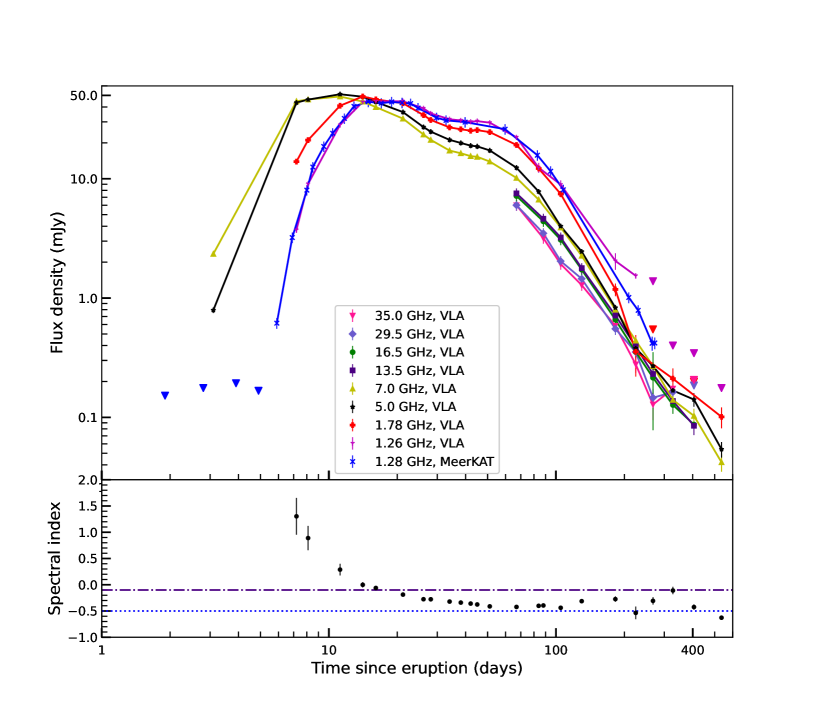
Figure 2: Top: Observed flux densities of V3890 Sgr spanning from day $2$ to day $536$ after the nova eruption. The upper limits in flux density are included as triangles. We take MJD = $58722.9$ as the date of the eruption ($t_{0}$). Bottom: spectral indices obtained by fitting a single power-law to multi-band data ($1.26-35$) GHz. The dash-dotted line in the lower panel represents $\alpha=-0.1$, the theoretically expected index of optically thin free-free emission. The dotted line represents $\alpha=-0.5$, the expected index of optically thin synchrotron emission.

Table 3: A summary of the radio flux densities of V3890 Sgr from MeerKAT and VLA observations.

$t-t_{0}$	$S\textunderscore 1.28$ (mJy)	$S\textunderscore 1.26$ (mJy)	$S\textunderscore 1.78$ (mJy)	$S\textunderscore 5.0$ (mJy)	$S\textunderscore 7.0$ (mJy)	$S\textunderscore 13.5$ (mJy)	$S\textunderscore 16.5$ (mJy)	$S\textunderscore 29.5$ (mJy)	$S\textunderscore 35.0$ (mJy)	Spectral
(Days)										index ($\alpha$)
1.9	$<$ 0.15
2.8	$<$ 0.18
3.1				0.79 $\pm$ 0.04	2.35 $\pm$ 0.12
3.9	$<$ 0.19
4.9	$<$ 0.18
5.9	0.62 $\pm$ 0.06
6.9	3.22 $\pm$ 0.32
7.2		3.73 $\pm$ 0.21	13.94 $\pm$ 0.70	43.48 $\pm$ 2.17	44.62 $\pm$ 2.23					1.30 $\pm$ 0.35
8.0	8.03 $\pm$ 0.80
8.1		9.06 $\pm$ 0.46	21.10 $\pm$ 1.06	46.09 $\pm$ 2.31	46.17 $\pm$ 2.31					0.90 $\pm$ 0.22
8.5	12.53 $\pm$ 1.25
9.5	18.65 $\pm$ 1.87
10.4	24.08 $\pm$ 2.41
11.2		28.30 $\pm$ 1.42	40.97 $\pm$ 2.05	51.11 $\pm$ 2.56	48.93 $\pm$ 2.45					0.29 $\pm$ 0.11
11.7	32.03 $\pm$ 3.21
12.9	40.44 $\pm$ 4.05
14.1		44.15 $\pm$ 2.21	48.95 $\pm$ 2.45	48.74 $\pm$ 2.44	44.35 $\pm$ 2.22					0.00 $\pm$ 0.05
14.9	44.20 $\pm$ 4.42
16.1		44.67 $\pm$ 2.24	46.26 $\pm$ 2.31	44.01 $\pm$ 2.20	39.89 $\pm$ 2.00					$-$0.06 $\pm$ 0.03
17.0	43.0 $\pm$ 4.30
18.9	44.07 $\pm$ 4.41
21.0	43.35 $\pm$ 4.34
21.2		44.66 $\pm$ 2.24	42.95 $\pm$ 2.15	36.23 $\pm$ 1.81	31.92 $\pm$ 1.60					$-$0.19 $\pm$ 0.02
21.9	42.68 $\pm$ 4.27
24.7	39.18 $\pm$ 3.92
26.1		38.89 $\pm$ 1.95	34.18 $\pm$ 1.71	27.12 $\pm$ 1.36	23.49 $\pm$ 1.18					$-$0.28 $\pm$ 0.02
28.1		35.30 $\pm$ 1.77	31.10 $\pm$ 1.56	24.83 $\pm$ 1.24	21.18 $\pm$ 1.06					$-$0.28 $\pm$ 0.03
29.8	32.49 $\pm$ 3.25
32.8	30.88 $\pm$ 3.10
34.0		31.53 $\pm$ 1.58	26.97 $\pm$ 1.35	21.19 $\pm$ 1.06	17.24 $\pm$ 0.86					$-$0.32 $\pm$ 0.04
38.1		30.85 $\pm$ 1.54	25.99 $\pm$ 1.30	19.96 $\pm$ 1.00	16.36 $\pm$ 0.82					$-$0.34 $\pm$ 0.04
39.8	29.84 $\pm$ 2.99
42.1		30.09 $\pm$ 1.51	25.30 $\pm$ 1.27	18.95 $\pm$ 0.95	15.48 $\pm$ 0.77					$-$0.36 $\pm$ 0.03
45.0		30.41 $\pm$ 1.52	25.55 $\pm$ 1.28	18.68 $\pm$ 0.93	15.28 $\pm$ 0.76					$-$0.38 $\pm$ 0.03
51.1		29.53 $\pm$ 1.48	24.62 $\pm$ 1.23	17.29 $\pm$ 0.86	13.94 $\pm$ 0.70					$-$0.41 $\pm$ 0.03
59.7	26.04 $\pm$ 2.61
67.0		22.26 $\pm$ 1.12	19.21 $\pm$ 0.96	12.38 $\pm$ 0.62	10.17 $\pm$ 0.51	7.54 $\pm$ 0.75	7.17 $\pm$ 0.72	6.01 $\pm$ 0.60	5.99 $\pm$ 0.60	$-$0.42 $\pm$ 0.01
82.8	15.76 $\pm$ 1.58
83.9		12.39 $\pm$ 1.19	12.19 $\pm$ 0.69	7.81 $\pm$ 0.39	6.68 $\pm$ 0.34					$-$0.40 $\pm$ 0.04
88.0						4.62 $\pm$ 0.46	4.40 $\pm$ 0.44	3.49 $\pm$ 0.35	3.18 $\pm$ 0.32	$-$0.39 $\pm$ 0.03
94.7	11.56 $\pm$ 1.16
104.9		8.94 $\pm$ 0.74	7.46 $\pm$ 0.45	4.0 $\pm$ 0.20	3.9 $\pm$ 0.20	3.22 $\pm$ 0.32	3.08 $\pm$ 0.31	2.04 $\pm$ 0.21	1.93 $\pm$ 0.20	$-$0.44 $\pm$ 0.03
107.7	8.08 $\pm$ 0.81

• Here, $t_{0}$ is taken as 2019 August 27.9 UT (MJD = 58722.9).

Table 4: continued

A summary of MeerKAT and VLA observations of V3890 Sgr. $t-t_{0}$ $S\textunderscore 1.28$ (mJy) $S\textunderscore 1.26$ (mJy) $S\textunderscore 1.78$ (mJy) $S\textunderscore 5.0$ (mJy) $S\textunderscore 7.0$ (mJy) $S\textunderscore 13.5$ (mJy) $S\textunderscore 16.5$ (mJy) $S\textunderscore 29.5$ (mJy) $S\textunderscore 35.0$ (mJy) Spectral (Days) index ($\alpha$) 129.8 2.45 $\pm$ 0.13 2.26 $\pm$ 0.12 1.78 $\pm$ 0.18 1.73 $\pm$ 0.17 1.45 $\pm$ 0.15 1.28 $\pm$ 0.13 $-$0.32 $\pm$ 0.01 182.6 2.05 $\pm$ 0.32 1.18 $\pm$ 0.14 0.83 $\pm$ 0.04 0.80 $\pm$ 0.04 0.72 $\pm$ 0.07 0.66 $\pm$ 0.07 0.55 $\pm$ 0.06 0.59 $\pm$ 0.07 $-$0.28 $\pm$ 0.05 209.2 1.01 $\pm$ 0.11 224.5 1.54 $\pm$ 0.08 0.36 $\pm$ 0.14 0.38 $\pm$ 0.02 0.44 $\pm$ 0.03 0.39 $\pm$ 0.04 0.35 $\pm$ 0.04 0.35 $\pm$ 0.05 0.28 $\pm$ 0.04 $-$0.10 $\pm$ 0.06 230.1 0.79 $\pm$ 0.08 265.1 0.42 $\pm$ 0.06 267.4 $<$1.38 $<$ 0.55 0.27 $\pm$ 0.02 0.27$\pm$ 0.02 0.23 $\pm$ 0.03 0.22 $\pm$ 0.14 0.15 $\pm$ 0.03 0.13 $\pm$ 0.03 $-$0.32 $\pm$ 0.07 272.3 0.42 $\pm$ 0.05 327.3 $<$ 0.40 0.21 $\pm$ 0.05 0.17 $\pm$ 0.02 0.14 $\pm$ 0.02 0.14 $\pm$ 0.02 0.13 $\pm$ 0.02 0.16 $\pm$ 0.04 0.17 $\pm$ 0.05 $-$0.11 $\pm$ 0.07 405.1 $<$ 0.35 $<$ 0.55 0.14 $\pm$ 0.02 0.10 $\pm$ 0.02 0.09 $\pm$ 0.01 0.09 $\pm$ 0.01 $<$ 0.19 $<$ 0.21 $-$0.41 $\pm$ 0.11 535.7 $<$0.18 0.10 $\pm$ 0.02 0.05 $\pm$ 0.01 0.04 $\pm$ 0.01 $-$0.63 $\pm$ 0.01

• Here, $t_{0}$ is taken as 2019 August 27.9 UT (MJD = 58722.9).

2.4 Radio spectral evolution

To determine the spectral evolution of V3890 Sgr, the data are fit assuming a simple power law using the method of least-squares. Measurements of the spectral index ($\alpha$ where $S_{\nu}~{}\propto~{}\nu^{\alpha}$) are presented in Figure 2 and Figure 3. During the early times (e.g., on day $11.2$), the flux density rises towards higher frequency, giving $\alpha=0.29$, an indicator of optically thick emission. Around the radio light curve maximum, e.g., on day $21$ the spectrum switches to rising towards lower frequency, and is well described by a power law with slope $\alpha=-0.2$.

The spectrum continues to steepen ($\alpha$ becomes more negative,) with time, as shown on day $67$ where $\alpha=-0.4$. On day $327$, the spectrum is flat $\alpha=-0.1$) indicative of optically thin free-free emission, however on day $534$, the spectrum rises steeply again towards lower frequencies and can be fit with a single power-law such that $\alpha=-0.6$, an indication of optically thin synchrotron emission. A mixture of optically thin free-free emission and synchrotron emission has also been observed in other novae such as V445 Pup (Nyamai et al., 2021) and V1535 Sco (Linford et al., 2017).

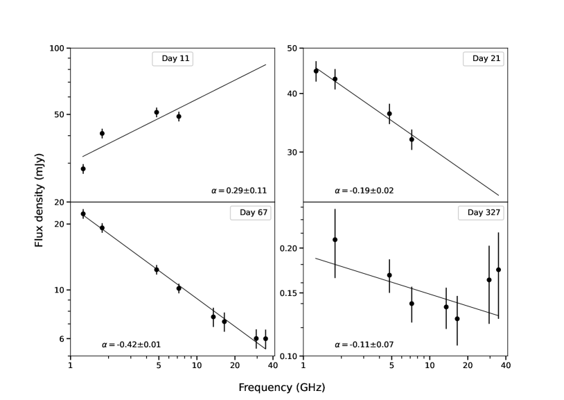
Figure 3: Spectral evolution of V3890 Sgr after the $2019$ eruption. The time since eruption and $\alpha$ is given for each fit represented by a solid line.

2.5 H i $21$-cm absorption measurements towards V3890 Sgr

The distance to V3890 Sgr is not well constrained, with estimates ranging from $4.4$ kpc to $9.0$ kpc using different methods (Schaefer, 2010; Munari & Walter, 2019a; Orio et al., 2020; Mikołajewska et al., 2021). Following the latest eruption, Munari & Walter (2019a) determined a reddening of $E(B-V)=0.56$ mag using absorption features of optical spectral lines. Comparing this value with the three-dimensional interstellar reddening maps of Green et al. (2019) and Lallement et al. (2014), they estimate a distance of $>4.5$ kpc. Using the surface temperature and the size of the companion star, a black body distance of $7$ kpc is derived to the nova (Schaefer, 2010). This method relies on the orbital period of the system and assumes that the companion star fills its Roche lobe (which is far from certain in the case of a symbiotic binary).

Since estimates of the distance to V3890 Sgr vary based on different observations, an attempt is made here to further constrain the distance using H i absorption along the line-of-sight to the nova (see Chauhan et al. 2021 for more details about H i absorption with MeerKAT). The epochs used to obtain the H i spectrum towards V3890 Sgr include radio detections of the nova when it was at its brightest ($>30$ mJy). Figure 4 shows the average MeerKAT H i spectrum towards V3890 Sgr, compared with the average of seven reference sources (indicated by the blue spectrum in Figure 4) which have been offset for clarity. These reference sources are presumably background extragalactic sources, and their spectra were averaged together to yield optimal S/N. These spectra were constructed by taking an inverse-variance weighted average over spectra from seven epochs observed with MeerKAT. Line-of-sight absorption through Galactic H i clouds is detected towards V3890 Sgr. By identifying distinct kinematic components in the H i spectrum, and comparing with the spectrum of reference sources, an attempt is made to determine the distance to V3890 Sgr.

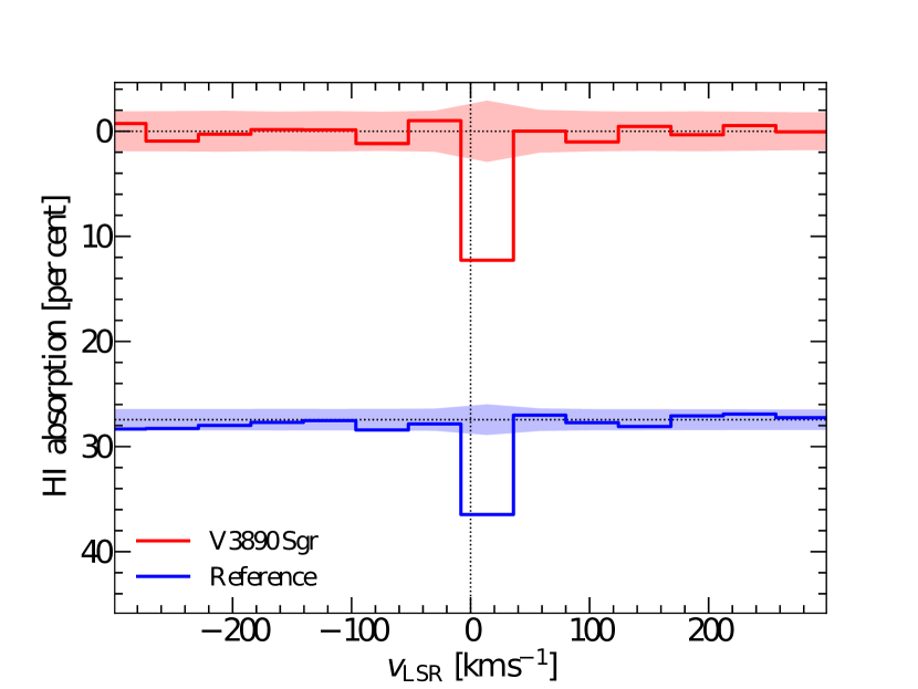
Figure 4: H i absorption spectrum showing an absorption between $-8~{}\textrm{km~{}s}^{-1}$ and $36~{}\textrm{km~{}s}^{-1}$ with respect to the local standard of rest. The spectrum of V3890 Sgr is plotted in red colour, and compared to an averaged spectrum of reference sources in blue colour. The shaded regions denote the noise level at $3\sigma$.

H i absorption at the level of $12\%$ is clearly detected in both the spectra of V3890 Sgr and the reference sources. In both cases, the absorption is at a velocity of $14\pm 22~{}\textrm{km~{}s}^{-1}$, but is unfortunately unresolved by the data obtained in the MeerKAT 4k correlator mode. At the time of the observations, the $32$k correlator mode was not yet available. Absorption is detected at velocities lower than $36~{}\textrm{km~{}s}^{-1}$, corresponding to kinematic distances greater than $4.44^{+0.34}_{-0.31}~{}\textrm{kpc}$ (using a Monte Carlo technique by Wenger et al., 2018). This estimate is similar to the distance value obtained using interstellar reddening as discussed earlier. Therefore, the distance constraint for this nova is consistent with being greater than $4.4$ kpc. The absolute magnitude in the $V$ filter and bolometric magnitude measurements give distance estimates of $8.75$ and $9$ kpc respectively (Mikołajewska et al., 2021). A distance of $9$ kpc is thus adopted for calculations in this work.

3 Discussion

3.1 Radio emission from V3890 Sgr is synchrotron dominated

The radio emission of novae embedded in the winds of giant stars is dominated by synchrotron emission, as observed in systems such as RS Oph (Taylor et al., 1989; O’Brien et al., 2006; Rupen et al., 2008; Sokoloski et al., 2008; Eyres et al., 2009), V745 Sco (Kantharia et al., 2016) and V1535 Sco (Linford et al., 2017). The non-thermal radio emission is the result of the ejecta interacting with the pre-existing circumstellar medium. A nova shock wave moving outwards populates a thin region of shocked circumstellar material with accelerated particles required for non-thermal emission. The evolution of the shock wave in symbiotic novae is similar to that of SNe following an explosion (e.g., Chevalier, 1982b; O’Brien et al., 2006). The radio luminosity increases as the optically thick emitting region expands. As the emitting region expands, the free-free optical depth from the ionized red giant wind ahead of the shock decreases, and the emission becomes optically thin. The radio luminosity peaks when $\tau=1$, and then decays as the expanding shock wave decelerates in velocity and the surrounding medium drops in density (Chevalier, 1982b).

The radio light curve of V3890 Sgr evolves through the three phases of rise, peak and decay within months following the nova eruption, and is similar to V745 Sco (e.g., Kantharia et al., 2016). The radio spectra of V3890 Sgr during the rise phase of the light curve yield a spectral index of $\alpha\approx 1.3$, consistent with optically thick emission. After the radio peak, the spectral index is steep and converges to $\alpha=-0.3$ at late times of light curve evolution (see Figure 2 and Table 3), an indication of optically thin synchrotron emission. Similar values of $\alpha$ are observed in sources that are strong synchrotron emission emitters such as SNe and SN remnants (Weiler et al., 2002; Green et al., 2019) and the helium nova V445 Pup (Nyamai et al., 2021).

To further constrain the type of emission from V3890 Sgr, the brightness temperature is determined by estimating the size of the emitting region (Nyamai et al., 2021; Chomiuk et al., 2021). To determine the angular size of the emitting region, a spherically symmetric shock wave expanding at $\approx 4200~{}\textnormal{km~{}s}^{-1}$ since $t_{0}$ is assumed (Strader et al., 2019). Using flux densities observed at $1.28$ GHz ($23$ cm), the estimated brightness temperatures on the first $200$ days are $\gg 10^{5}$ K as shown in Figure 5, a strong indicator of non-thermal emission (Chomiuk et al., 2021). The brightness temperature after day $200$ declines to $\approx 10^{4}$ K. However, we note that the actual angular size of the emitting region may be substantially smaller than our estimated size of the emitting region, since the shock wave decelerates as it interacts with the red giant wind. The implication is that the brightness temperatures shown in Figure 5 are lower limits. The spectral evolution and brightness temperatures indicate that the radio emission from V3890 Sgr is synchrotron dominated, produced in a manner similar to that in SNe, where the radio light curve also evolves on timescales of weeks to months (Weiler et al., 2002).

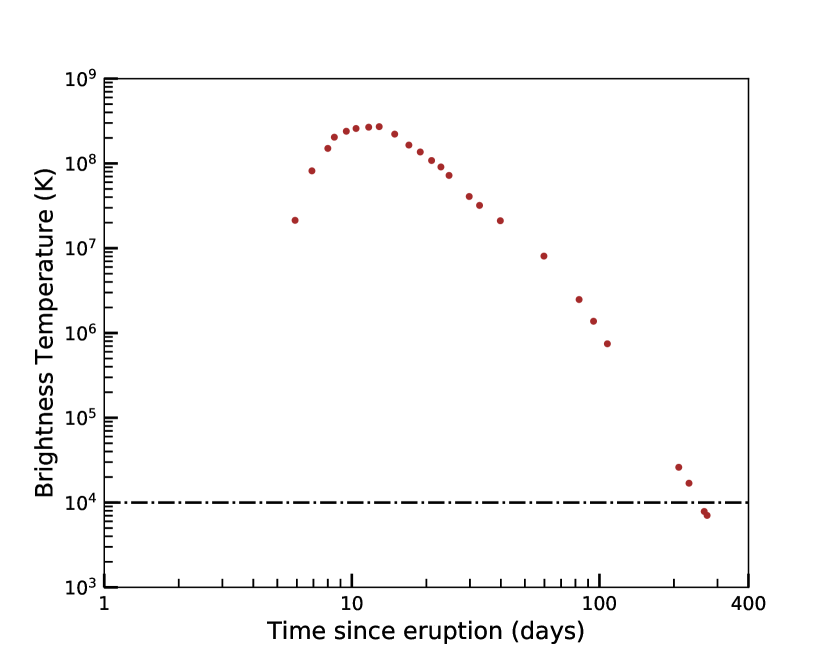
Figure 5: Brightness temperature of V3890 Sgr following the $2019$ eruption, estimated assuming a constant shock velocity of $4200$ $\textnormal{km~{}s}^{-1}$, and flux densities of the $1.28$ GHz observing frequency.

3.2 A model for synchrotron emission from nova blast waves

In an environment where the nova ejecta interact with a dense surrounding medium, radio emission can be used to probe the external surrounding medium and determine its density profile, as is commonly done in radio SNe (e.g., Weiler et al., 2002). The radial profile depends on the mass loss from the companion star and its shaping by binary interaction (e.g., Mohamed et al., 2015; Ji et al., 2013). An interaction of the nova ejecta with the companion’s wind will accelerate particles to high energies through diffusive shock acceleration (Blandford & Ostriker, 1978; Bell, 1978) and amplify the shock magnetic field (Bell, 2004), producing synchrotron radiation. The interaction produces a forward shock which drives into the pre-existing circumstellar material and a reverse shock driving into the ejecta (Chevalier, 1982a; Reynolds, 2017). The radius of discontinuity $R_{\textrm{cd}}$ separates the forward- and reverse-shocked regions. The evolution of the shock fronts depends on the density structure of the nova ejecta ($\rho_{\textrm{ej}}$) and that of the surrounding medium ($\rho_{\textrm{CSM}}$; Chevalier 1982a; Tang & Chevalier 2017).

To interpret the radio luminosity from V3890 Sgr, this double shock system is considered. Shock wave dynamics have been observed in X-rays for recurrent novae, where the most notable characteristics of the shocked ejecta are high temperatures, $\gtrsim 10^{7}$ K, which decrease with time as the shock decelerates (e.g., Sokoloski et al., 2006; Bode et al., 2006). Immediately following its $2019$ eruption, V3890 Sgr produced hard X-rays, which were attributed to the nova outflow impacting the red-giant wind (Sokolovsky et al., 2019; Orio et al., 2020; Page et al., 2020; Singh et al., 2021). More evidence of shocks in V3890 Sgr comes from the presence of high-ionization emission lines in optical and infrared spectra (Munari & Walter, 2019b; Evans et al., 2022).

A formalism for predicting synchrotron emission from shocks is put forward by Chevalier (1982b). Above a minimum energy $E_{\rm min}$, the energy spectrum of relativistic electrons can be described by a power law distribution, $N(E)=N_{0}~{}E^{-p}$ where $N_{0}$ is a constant, $N(E)$ is the number of particles with energy $E$, and $p$ is the power law index of the energy spectrum. The energy of a relativistic electron is $E=\gamma m_{e}c^{2}$, where $\gamma$ and $m_{e}$ are the Lorentz factor and mass of an electron, respectively. For the non-relativistic shock velocities observed in V3890 Sgr, we assume that $E_{\rm min}$ is the rest-mass of the electron. The optically thin synchrotron spectrum produced by a power law distribution of electrons is also a power law, $L_{\nu}\propto\nu^{-(p-1)/2}$, so that the spectral index $\alpha=-(p-1)/2$. For V3890 Sgr, an average value of $\alpha\approx-0.3$ is measured in the optically thin limit of the radio light curve. This translates to $p=1.6$. Theoretically, in diffusive shock acceleration, the spectral index of relativistic particles $p$ is predicted to be between $2$ and $2.5$ (Bell, 1978; Blandford & Ostriker, 1978). However, for novae, $p$ is observed in the range of $1.2$ and $2$ (Eyres et al., 2009; Finzell et al., 2018; Nyamai et al., 2021). This could imply that relativistic electrons in novae are more evenly distributed between low and high energies, or the magnetic fields and particle density are not uniformly distributed leading to complex optical depth effects (Vlasov et al., 2016). For the non-relativistic shocks in novae, the minimum energy is taken to be the rest mass energy of the electron ($\gamma_{\rm min}=1$; Chevalier 1998).

The post-shock energy density is described as $U_{\textrm{shock}}\approx\rho_{\textrm{CSM}}\,V_{\textrm{shock}}^{2}$, where $\rho_{\textrm{CSM}}$ is the density of the material being shocked and $V_{\textrm{shock}}$ is the velocity of the forward shock. In Chevalier’s model, it is assumed that a fraction of the post-shock energy density is transferred to the accelerated electrons and the amplified magnetic field. Therefore, the energy density in relativistic electrons is $U_{e}=\epsilon_{e}\,\rho_{\textrm{CSM}}\,V_{\textrm{shock}}^{2}$, and the energy density in the magnetic field is $U_{B}=\epsilon_{B}\,\rho_{\textrm{CSM}}\,V_{\textrm{shock}}^{2}$. The efficiency factors $\epsilon_{e}$ and $\epsilon_{B}$ are used to describe the fraction of the post-shock energy in the form of relativistic electrons and amplified magnetic fields, respectively. The normalization for the electron energy spectrum can be expressed as:

$$N_{0}=\epsilon_{e}\,\rho_{\textrm{CSM}}\,V_{\textrm{shock}}^{2}\,(p-2)\,E_{\rm min}^{p-2}$$ (2)

in cgs units; this expression is valid for $p>2$.

Chevalier (1998) expresses the flux density of synchrotron emission at frequency $\nu$ as:

$$S_{\nu}=1.8~{}\times~{}10^{-22}~{}\bigg{(}\frac{\pi~{}R^{2}}{D^{2}}\bigg{)}~{}\frac{C_{5}}{C_{6}}~{}B^{-0.5}~{}\nu^{2.5}\Bigg{(}1-\textrm{exp}\bigg{[}-\frac{\nu}{\nu_{1}}^{\frac{-p-4}{2}}\bigg{]}\bigg{)}~{}\textrm{mJy}.$$ (3)

Constants $C_{5}$ and $C_{6}$ are determined as a function of $p$ (Pacholczyk, 1970). For V3890 Sgr, we take $p=2.1$ as this modelling formalism require $p>2.1$. Therefore, the values $C_{5}=1.37~{}\times~{}10^{-23}$ and $C_{6}=8.61~{}\times~{}10^{-41}$ for $p=2.1$ are used here. $R$ is the radius of the blast wave, and $D$ is the distance to the nova. $B$ is the post-shock magnetic field strength and is given by $B=\sqrt{8\,\pi\,U_{B}}$. $\nu_{1}$ is the frequency at which the optical depth to synchrotron self-absorption (SSA) is equal to unity, given as

$$\nu_{1}=1.3~{}\times~{}10^{19}\times\bigg{(}\frac{4}{3}f~{}R~{}C_{6}~{}N_{0}\bigg{)}^{\frac{2}{p+4}}~{}\times~{}B^{(\frac{p+2}{p+4})}~{}\textrm{Hz}.$$

The synchrotron emitting region is assumed to be between the forward shock and the contact discontinuity; its volume filling factor is quantified as $f$. We estimate the value of $f=0.88$ using the approximations of the forward shock radius and the contact discontinuity radius given in Tang & Chevalier (2017). For the blast wave evolution described in §3.3, the forward shock radius is twice that of the contact discontinuity.

Radio synchrotron luminosity may increase at early times due to SSA or free-free absorption by the ionized gas ahead of the forward shock, depending on the amplified magnetic field, the density of the external medium and the shock wave velocity (Chevalier, 1998; Weiler et al., 1986). It has been shown that free-free absorption is dominant for slow shock wave velocities ($\lesssim 10^{4}~{}\textrm{km~{}s}^{-1}$) while SSA is the dominant source of opacity for faster blast waves (Chevalier, 1998; Panagia et al., 2006). In cases where the optical depth is dominated by an ionized wind-like medium (as described in §3.3.2) ahead of the shock, the free-free optical depth is defined by Chevalier (1981) as

$$\begin{split}\tau_{\textrm{ff}}&=0.005\bigg{(}\frac{{\dot{M}}}{10^{-6}~{}\textrm{M}_{\odot}~{}\textrm{yr}^{-1}}\bigg{)}^{2}\times\bigg{(}\frac{V_{\textrm{wind}}}{10~{}\textrm{km~{}s}^{-1}}\bigg{)}^{-2}\times\bigg{(}\frac{\nu}{1.4~{}\textrm{GHz}}\bigg{)}^{-2}\\ &\times\bigg{(}\frac{R_{\textrm{shock}}}{2\times 10^{16}~{}\textrm{cm}}\bigg{)}^{-3}\end{split}$$ (4)

3.3 The dynamics of the blast wave

To predict the radio luminosity of a nova interacting with circumbinary material, we must know the radius and velocity of the blast wave. These depend on the density and velocity structure of the nova ejecta, along with the density profile of the circumbinary material.

3.3.1 The density structure of the nova ejecta

The unshocked material of the nova envelope is commonly described as expanding freely and homologously, such that $V(r)\propto r$ where $V$ is the expansion velocity and $r$ is radial distance from the white dwarf. In this case, the ejecta would show a range of velocities with the inner ejecta characterised by low velocities and the outer ejecta expanding fastest. Based on the modelling of nova remnants, the density profiles of the ejecta can be described by a power law distribution, $\rho_{\textrm{ej}}\propto r^{-n}$ with inner ejecta having $n=~{}2$ or $3$ and outer ejecta having $n$ between $10$ and $20$ (e.g., Hauschildt et al., 1997). Only a tiny fraction of the ejecta mass is found in the outer parts characterised by a steep power law (and this mass will be swept up very quickly, in just a few hours), so a shallow power law is adopted to describe the ejecta density profile of V3890 Sgr, such that $n~{}=~{}2$. The kinetic energy of the nova ejecta is therefore the integral of the density profile with an homologous expansion such that

$$E=0.17\times\bigg{(}\frac{M_{\textrm{ej}}}{{\textnormal{M}}_{\odot}}\bigg{)}\times\bigg{(}\frac{V^{3}_{\textrm{max}}}{{\textrm{cm~{}s}^{-1}}}-\frac{V^{3}_{\textrm{min}}}{{\textrm{cm~{}s}^{-1}}}\bigg{)}/\bigg{(}\frac{V_{\textrm{max}}}{{\textrm{cm~{}s}^{-1}}}-\frac{V_{\textrm{min}}}{{\textrm{cm~{}s}^{-1}}}\bigg{)}^{-1}~{}\textrm{erg}$$ (5)

where $M_{\textrm{ej}}$ is the mass of the nova ejecta, $V_{\textrm{max}}$ is the maximum ejecta velocity and $V_{\textrm{min}}$ is the minimum ejecta velocity.

Observationally, the ejected masses of symbiotic recurrent novae are in the range of $10^{-7}$–$10^{-6}~{}{\textnormal{M}}_{\odot}$ (O’Brien et al., 1992; Anupama & Sethi, 1994; Sokoloski et al., 2006; Orlando et al., 2017). After the 1990 eruption of V3890 Sgr, the optical light curve at $V$ band declined by three magnitude in $14$ days (Schaefer, 2010). After the $2019$ eruption, the optical light curve also shows a fast decline (see Figure 1). Such a fast decline is expected for nova envelopes with mass of $<10^{-6}~{}\textnormal{M}_{\odot}$ (Yaron et al., 2005). Furthermore, the same rapid decay of the optical light curve is observed in RS Oph, where its ejected nova envelope is estimated to be $(10^{-7}\leq~{}M_{\textrm{ej}}\leq 10^{-6})~{}\textnormal{M}_{\odot}$ (e.g., O’Brien et al., 1992; Sokoloski et al., 2006). More evidence of a low-mass ejected envelope in V3890 Sgr is based on the fast nova evolution where high-ionization lines appear in the spectra $\approx 18$ day following the $1990$ eruption (Anupama & Sethi, 1994). Anupama & Sethi use Balmer emission line fluxes to estimate the mass of the nova envelope as $\approx 10^{-7}~{}\textnormal{M}_{\odot}$. In our analysis we consider ejecta masses in the range $10^{-7}$–$10^{-5}~{}{\textnormal{M}}_{\odot}$.

3.3.2 The density structure of the circumstellar medium

The simplest model for the circumstellar material is to assume the companion star is expelling a spherically symmetric wind with constant velocity and mass-loss rate. The density distribution of the medium is then described as

$$\rho_{\textrm{CSM}}=\frac{\dot{M}}{4\pi V_{\textrm{wind}}}r^{-2}$$ (6)

where $\dot{M}$ is the mass loss rate, $V_{\textrm{wind}}$ is the velocity of the red giant wind, and $r$ is the distance from the companion binary. Without prior knowledge of the distribution of circumstellar material, this spherical distribution of the red giant wind is assumed for V3890 Sgr. It is however noted that non-spherical distribution of material is common in symbiotic recurrent systems (Walder et al., 2008; Booth et al., 2016a). Furthermore, the two components observed in the emission line profiles of V3890 Sgr following the 1990 eruption indicate that the nova remnant is non-spherical (Anupama & Sethi, 1994). A spherical assumption considered here is therefore a simplistic approach.

3.3.3 Radius and velocity of the shock front

The time evolution of a shock wave propagating through the red giant wind is divided into two phases. During the first phase, when the mass of the nova envelope ($M_{\textrm{ej}}$) is much larger than that of the swept-up surrounding medium ($M_{\textrm{sw}}$), the shock is in free expansion. As the mass of the swept up material increases such that $M_{\textrm{sw}}~{}>M_{\textrm{ej}}$, the nova envelope enters a second phase of evolution referred to as the Sedov-Taylor phase. For spherical nova ejecta with a power-law density profile ($\rho_{\textrm{ej}}\propto r^{-2}$) interacting with circumstellar medium of density, $\rho_{\textrm{CSM}}\propto r^{-2}$, self-similar solutions are determined for the evolution from a free expansion phase to the adiabatic expansion phase, as shown in Table $1$ of Tang & Chevalier (2017). For the purposes of this analysis, we assume that the red giant and white dwarf are co-located at the center of the red giant wind, a valid assumption over the course of the radio light curve because the shocked ejecta expand outside the binary system within the first day of eruption.

Tang & Chevalier (2017) present expressions for the radius and velocity of the forward shock with time, given as $R_{\textrm{shock}}=R_{ch}\times R^{*}_{b}$, $V_{\textrm{shock}}=V_{ch}\times V^{*}_{b}$, and $t=t_{ch}\times t^{*}$. Here $R_{ch}$, $V_{ch}$, and $t_{ch}$ are the characteristic radius, velocity and time, respectively:

$$\begin{split}R_{ch}&=12.9\times\bigg{(}\frac{M_{\textrm{ej}}}{\textrm{M}_{\odot}}\bigg{)}\times\bigg{(}\frac{\overset{\hbox{\tiny$\bullet$}}{M}}{10^{-5}~{}\textrm{M}_{\odot}\textrm{yr}^{-1}}\bigg{)}^{-1}\\ &\times\bigg{(}\frac{V_{\textrm{wind}}}{10~{}\textrm{km~{}s}^{-1}}\bigg{)}~{}\textrm{pc}\end{split}$$ (7)

$$\begin{split}t_{ch}&=1772\times\bigg{(}\frac{E}{10^{51}~{}\textrm{erg}}\bigg{)}^{-0.5}\times\bigg{(}\frac{M_{\textrm{ej}}}{\textrm{M}_{\odot}}\bigg{)}^{1.5}\times\bigg{(}\frac{\overset{\hbox{\tiny$\bullet$}}{M}}{10^{-5}~{}\textrm{M}_{\odot}\textrm{yr}^{-1}}\bigg{)}^{-1}\\ &\bigg{(}\frac{V_{\textrm{wind}}}{10~{}\textrm{km~{}s}^{-1}}\bigg{)}~{}\textrm{yr}\end{split}$$ (8)

$$\begin{split}v_{ch}=7118.24\times\bigg{(}\frac{E}{10^{51}~{}\textrm{erg}}\bigg{)}^{0.5}\times\bigg{(}\frac{M_{\textrm{ej}}}{\textrm{M}_{\odot}}\bigg{)}^{-0.5}~{}\textrm{km~{}s}^{-1}\end{split}$$ (9)

$R^{*}_{b}$, $V^{*}_{b}$ are analytical dimensionless quantities defined by Tang & Chevalier (2017), and can be written as a function of $t^{*}=t/t_{ch}$ as

$$R^{*}_{b}=2.91489\times t^{*}(1+9.36843t^{*0.567})^{-0.5882}$$ (10)

$$V^{*}_{b}=\frac{dR^{*}}{dt^{*}}=(2.91489~{}+~{}18.2t^{*0.567})(1~{}+~{}9.36843t^{*0.567})^{-1.5882.}$$ (11)

The predicted radius ($R_{\textrm{shock}}$) and velocity ($V_{\textrm{shock}}$) of the blast wave are shown in Figure 6. The radius and velocity of the shock depend on the ejecta mass ($\approx 10^{-5}-10^{-7}~{}\textrm{M}_{\odot}$) and kinetic energy of the nova ejecta, along with the density of the circumbinary material (i.e., ${\dot{M}}/V_{\textrm{wind}}$). The shock radius first grows linearly with $t$ and later as $t^{0.67}$. Similarly, the shock wave velocity first remains at a near-constant value but decreases as $t^{-0.33}$ at later times. The flux densities depend on these quantities, but also on the distance to the nova, $\epsilon_{e}$, and $\epsilon_{B}$. We tweaked $M_{\textrm{ej}}/E$ to yield maximum expansion velocities at early times (i.e., during free expansion; Figure 6) consistent with the maximum ejecta velocity of $\approx 4200~{}\textrm{km~{}s}^{-1}$, as estimated from optical spectroscopy (Strader et al., 2019).

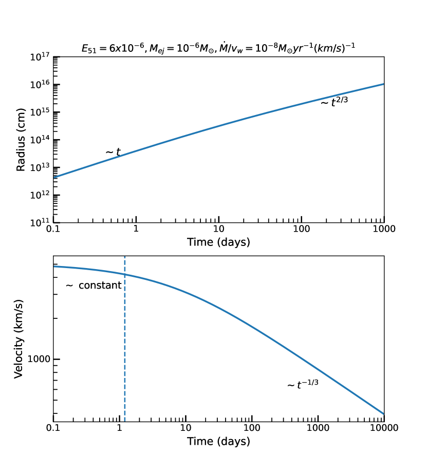
Figure 6: Top: Radial evolution for a nova forward shock interacting with a circumstellar material, assuming ejecta mass of 10^-6 M_⊙, kinetic energy $E=6\times 10^{45}$ erg, and $\dot{M}=10^{-7}$ M_⊙ yr^-1 for $V_{\rm wind}$ = 10 km s^-1. This represents the free expansion ($R_{\rm shock}\propto t$) and the Sedov-Taylor phase of the evolution ($R_{\rm shock}\propto t^{2/3}$). Bottom: Velocity evolution of the forward shock as it interacts with the surrounding medium. At the beginning of the evolution, during the free expansion phase, the velocity is constant. Later, the shock enters the Sedov-Taylor phase of evolution and $V_{\textrm{shock}}\propto t^{-1/3}$. The vertical dashed line represents the initial maximum velocity of $\approx 4200~{}\textrm{km~{}s}^{-1}$ of the nova ejecta on day $1.2$ after the nova eruption.

3.4 Modelling the radio light curve of V3890 Sgr

3.4.1 Constraining the mass of the ejected envelope

The radio light curve of V3890 Sgr is compared to the model used to explain non-thermal emission in supernova explosions (§3.2; Chevalier, 1998). The model depends on various input parameters, including: $p=2.1$, $V_{\textrm{wind}}=10~{}\textnormal{km~{}s}^{-1}$, and the distance to the nova ($9$ kpc). The velocity and radial profile of the expanding material are as discussed in §3.3.3.

First, we consider a range of $M_{\textrm{ej}}$ between $M_{\textrm{ej}}=10^{-5}~{}\textnormal{M}_{\odot}$ and $10^{-7}~{}\textnormal{M}_{\odot}$. Figure 7 shows model radio light curves for three different ejecta masses: $M_{\textrm{ej}}=10^{-5}~{}\textnormal{M}_{\odot}$, $10^{-6}~{}\textnormal{M}_{\odot}$, and $10^{-7}~{}\textnormal{M}_{\odot}$. In all three cases, we assume ${\dot{M}}=3.2~{}\times~{}10^{-8}~{}\textrm{M}_{\odot}~{}\textrm{yr}^{-1}$ for $V_{\textrm{wind}}=10~{}\textrm{km~{}s}^{-1}$ and $\epsilon_{e}=\epsilon_{B}=0.01$. The value of ${\dot{M}}$ is estimated based on the fit of the radio fluxes peak. For a particular value of $M_{\textrm{ej}}$, the kinetic energy is varied to yield a maximum velocity of $\approx 4200$ km s^-1 on day $1.2$ (Strader et al., 2019).

For model A (left panel of Figure 7), the synchrotron emission is significantly more luminous and longer lasting than the observations. With the parameters given in model B in Table 5, $M_{\textrm{ej}}=10^{-6}~{}\textnormal{M}_{\odot}$ agrees well with the data during the rise and peak of the radio emission (middle panel of Figure 7). For model C, the right panel of Figure 7, the radio light curve is less bright and the radio emission does not last very long. None of the models predict the decay phase of the radio light curve accurately. A discussion of why this is the case is included in §3.4.2.

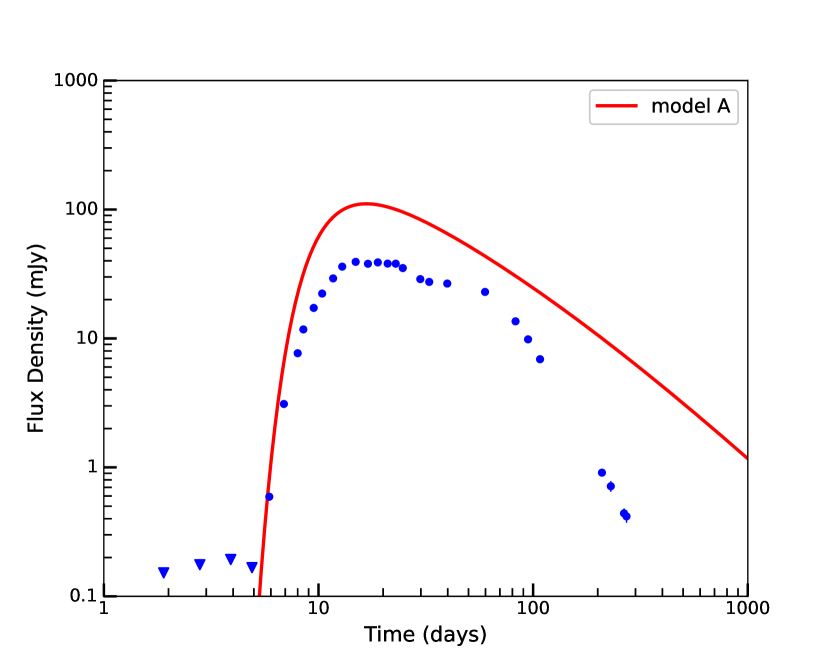
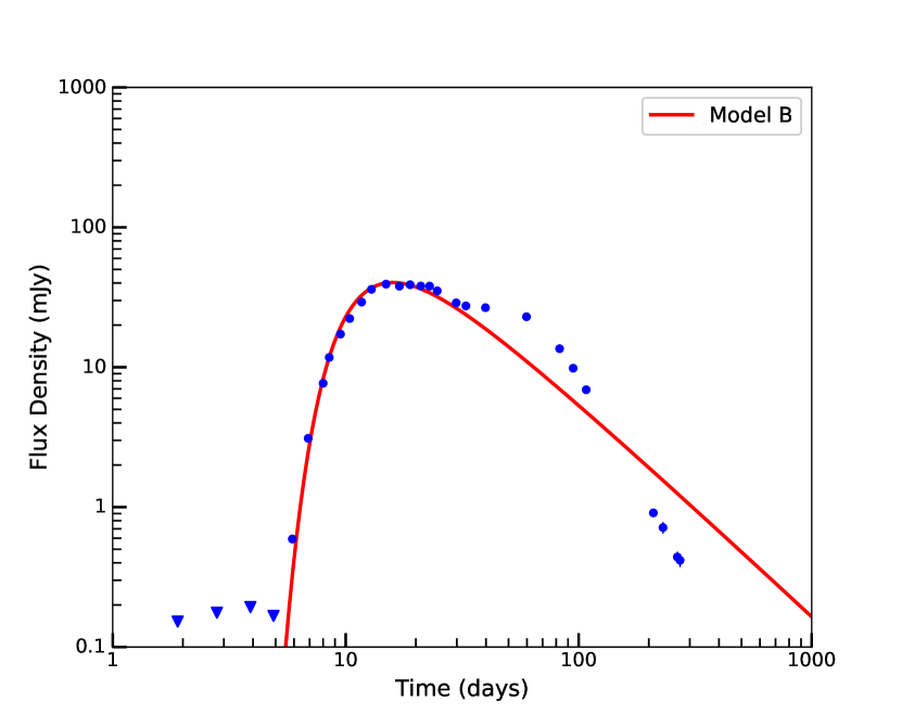
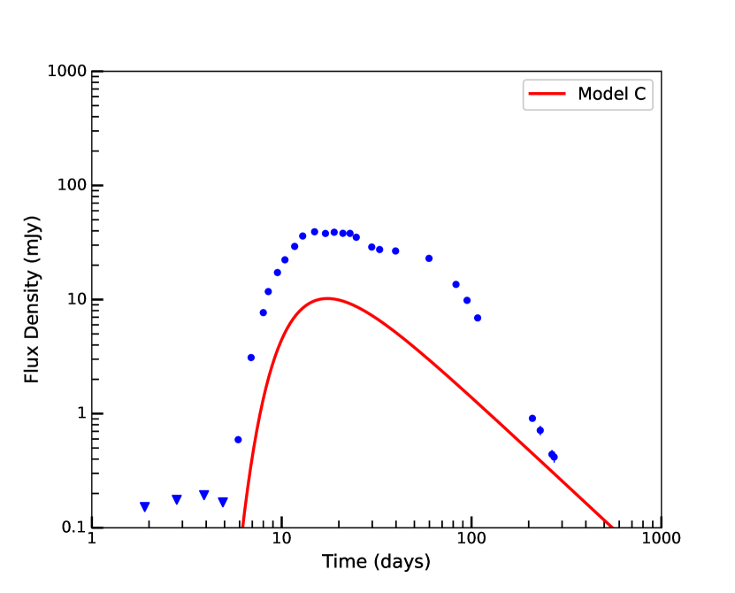
Figure 7: Models of radio emission produced by synchrotron emission undergoing free-free absorption are represented as red solid lines and superimposed on the MeerKAT $1.28$ GHz light curve of V3890 Sgr (blue points). The three panels correspond to different models as described in Table 5. For a particular value of $M_{\textrm{ej}}$, the kinetic energy is varied to yield a maximum velocity on day $1.2$. For model A (left panel) with $M_{\textrm{ej}}=10^{-5}~{}\textnormal{M}_{\odot}$, the synchrotron emission is significantly more luminous and longer lasting than the observations. The middle plot shows model B for $M_{\textrm{ej}}=10^{-6}~{}\textnormal{M}_{\odot}$, and is a good match to the observations during the rise and peak of the radio emission. The right plot represents model C for $M_{\textrm{ej}}=10^{-7}~{}\textnormal{M}_{\odot}$, and is not luminous enough to match the observations.

Table 5: Model parameters.

Model	Frequency	Kinetic energy	Ejecta mass	$\epsilon_{e}$	$\epsilon_{B}$	RG wind $\dot{M}$
	(GHz)	(erg)	($\textnormal{M}_{\odot}$)			($\textnormal{M}_{\odot}~{}\textnormal{yr}^{-1}$)
A	1.28	$4.5\times 10^{44}$	$10^{-5}$	0.01	0.01	$3.2\times 10^{-8}$
B	1.28	$6.0\times 10^{43}$	$10^{-6}$	0.01	0.01	$3.2\times 10^{-8}$
C	1.28	$1.4\times 10^{43}$	$10^{-7}$	0.01	0.01	$3.2\times 10^{-8}$
D	1.28	$4.5\times 10^{44}$	$10^{-5}$	0.004	0.004	$3.2\times 10^{-8}$
E	1.28	$1.4\times 10^{43}$	$10^{-7}$	0.01	0.1	$3.2\times 10^{-8}$
F	1.78	$6.0\times 10^{43}$	$10^{-6}$	0.01	0.01	$3.2\times 10^{-8}$
G	5.0	$6.0\times 10^{43}$	$10^{-6}$	0.01	0.01	$3.2\times 10^{-8}$
H	7.0	$6.0\times 10^{43}$	$10^{-6}$	0.01	0.01	$3.2\times 10^{-8}$

• Here we assume a wind velocity, $V_{\textrm{wind}}=10~{}\textrm{km~{}s}^{-1}$.

For the more massive ejection ($M_{\textrm{ej}}=10^{-5}~{}\textnormal{M}_{\odot}$) to not overpredict the radio flux densities, the model would require less energy in accelerated particles and amplified magnetic fields, such that $\epsilon_{e}=\epsilon_{B}=0.004$. This is consistent with estimates of particle acceleration implied by modelling of $\gamma$-ray emission from a symbiotic nova (e.g., Abdo et al., 2010). Additionally, Sarbadhicary et al. (2017) have also shown $\epsilon_{e}$ to be lower than $0.01$ in non-relativistic shocks. Adopting these values of $\epsilon_{e}$ and $\epsilon_{B}$ produces a model D shown in Figure 8 and tabulated in Table 5.

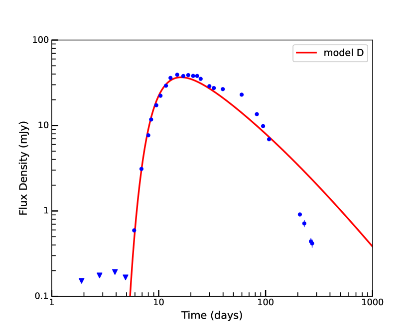
Figure 8: Model of radio emission produced by synchrotron emission undergoing free-free absorption (represented as the red solid line), superimposed on the MeerKAT light curve (blue points) for a massive ejection $M_{\textrm{ej}}=10^{-5}~{}\textnormal{M}_{\odot}$ with a shock that is less efficient at accelerating electrons and amplifying magnetic fields; see model D in Table 5 for details.

For the less massive ejection ($M_{\textrm{ej}}=10^{-7}~{}\textnormal{M}_{\odot}$) to not underpredict the radio flux densities, the model requires a high efficiency of either accelerating particles or amplifying magnetic fields, if not both. As $\epsilon_{B}$ is the more poorly constrained parameter (e.g., Chevalier & Fransson, 2006; Lundqvist et al., 2020), we let it vary while holding $\epsilon_{e}$ fixed, finding a good match to the observed light curve with $\epsilon_{e}=0.01$ and $\epsilon_{B}=0.1$ (Figure 9; Model E in Table 5). This produces a better fitting model compared to model C. However, since $\epsilon_{B}$ has been shown to vary significantly with values as low as $3~{}\times~{}10^{-3}$ (Lundqvist et al., 2020), this less massive ejection model should be considered with caution.

The most likely mass of the ejecta envelope is therefore, between $10^{-5}~{}\textnormal{M}_{\odot}$ and $10^{-6}~{}\textnormal{M}_{\odot}$. These values of ejecta mass are similar to those estimated in recurrent novae T Pyx (Nelson et al., 2014) and RS Oph (Pandey et al., 2022).

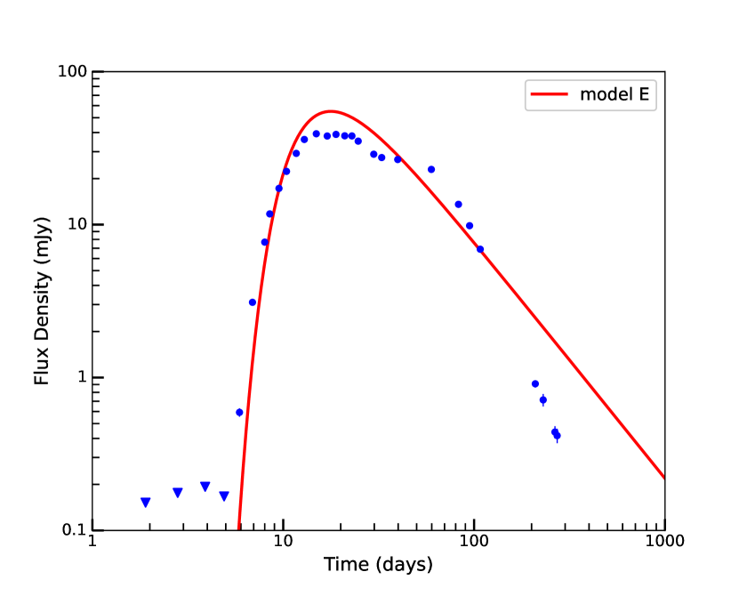
Figure 9: Model of radio emission produced by synchrotron emission undergoing free-free absorption represented (red solid line) superimposed on the MeerKAT light curve (blue points) for a less massive ejection $M_{\textrm{ej}}=10^{-7}~{}\textnormal{M}_{\odot}$ that is more efficient at amplifying the post-shock magnetic field; see model E in Table 5 for details.

The model of the first radio peak is compared to the VLA radio light curves at frequencies between $1.78$ GHz and $7$ GHz as shown in Figure 10.

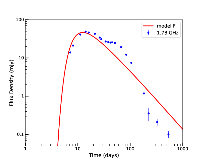
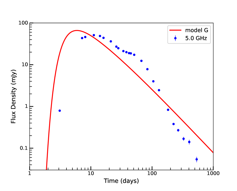
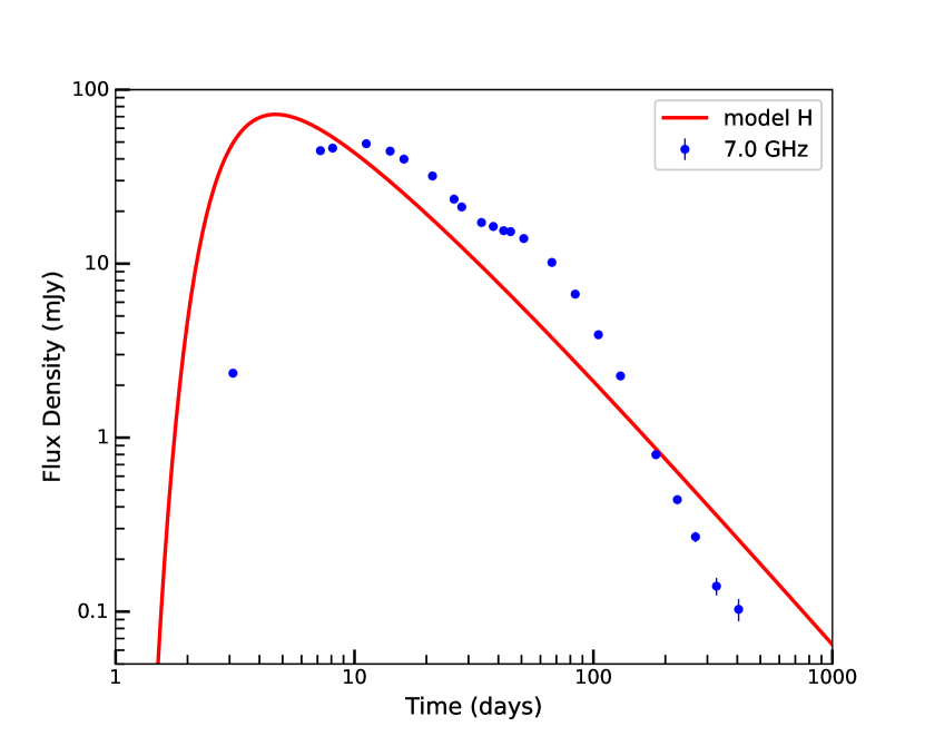
Figure 10: Models of radio emission produced by synchrotron emission undergoing free-free absorption are represented as red solid lines and superimposed on the VLA data (blue points) observed at frequencies $1.78$ GHz (left panel), $5.0$ GHz (middle) and $7.0$ GHz (right). The three panels from left to right represent models F, G, and H respectively (see Table 5).

At higher frequencies, the ejected material becomes optically thin faster for an homologous expanding material and thus provides information at smaller radii. By keeping the ejected mass and ${\dot{M}}$ at constant values of $10^{-6}~{}\textnormal{M}_{\odot}$ and ${\dot{M}}=3.2~{}\times 10^{-8}~{}\textrm{M}_{\odot}~{}\textrm{yr}^{-1}$, the MeerKAT model does not provide proper fits for any of the VLA radio light curves (see Figure 10). This implies that the CSM profile cannot be described with $\rho_{\textrm{C}SM}\propto r^{-2}$ at the regions closest to the compact object.

Even though the prediction of synchrotron luminosity is sensitive to the assumptions made, in all the cases presented above, the radio light curve provides an estimate of the mass-loss rate of the red-giant companion of $3.2\times 10^{-8}~{}\textnormal{M}_{\odot}~{}\textrm{yr}^{-1}$. Using radio observations and assuming spherically distributed ionized circumstellar material in symbiotic systems, Seaquist & Taylor (1990) determined $\overset{\hbox{\tiny$\bullet$}}{M}_{\textrm{w}ind}=10^{-7}\textnormal{~{}M}_{\odot}~{}\textnormal{yr}^{-1}$ for most red giant stars assuming $V_{\textrm{wind}}$= $10~{}\textrm{km~{}s}^{-1}$. However, studies of the most studied recurrent nova RS Oph imply a mass loss rate of $10^{-8}~{}\textnormal{M}_{\odot}~{}\textrm{yr}^{-1}$ (Vaytet et al., 2007; Van Loon, 2008). The mass-loss rate of V3890 Sgr estimated from its radio light curve is in the range of those found for red giants in symbiotic systems and RS Oph.

3.4.2 Explaining the second radio light curve peak

While our simple model of a $\rho_{\textrm{C}SM}\propto r^{-2}$ circumstellar medium fits the radio light curve rise and peak of V3890 Sgr well, the light curve then plateaus around days $\sim$30–60, in excess of the model (Figures 7–10; see also Figure 2). We call this excess emission the “second peak” of the radio light curve. Before day $17$, the radio flux is rising. During the decay phase of the radio light curve of V3890 Sgr, the flux densities can be described by a power law relationship with time such that $S_{\nu}\propto~{}t^{\beta}$. Around day $17$, after the first radio peak, the radio emission flattens such that $\beta=-0.5$. After the second peak, from day $60$ on, the radio flux density rapidly declines as $\beta=-2.8$, which is a steeper decay than predicted by our model with a $\rho_{\textrm{C}SM}\propto r^{-2}$ circumstellar medium. This standard model is described by $\beta=-1.3$ for the decline phase (Chevalier & Fransson, 2006).

The synchrotron luminosity produced when a nova remnant interacts with the circumstellar medium is expected to rise, peak and decay in a span of a few months (Kantharia, 2012). The radio luminosity in this framework decays during the optically thin phase of the radio light curve due to a decrease in circumbinary density and/or shock wave velocity (Weiler et al., 2002). This second peak cannot be explained by a single interaction with a spherically distributed wind-like circumstellar medium.

Double-peaked radio light curves have been observed previously in novae with giant companions, but on different timescales. For example the radio light curve of the $2006$ eruption of nova RS Oph showed a first peak around day $8$, which was followed by a second peak on day $40$ (Eyres et al., 2009). Based on its spectral evolution, the authors concluded that the radio emission from the nova is mixed thermal and non-thermal radiation. V1535 Sco is another symbiotic nova where the radio light curve shows several radio peaks with the first one recorded on day $25$ (Linford et al., 2017). The spectral evolution of V1535 Sco is also consistent with a mixture of thermal and non-thermal emission (Linford et al., 2017).

V3890 Sgr is the first symbiotic recurrent nova where the second radio bump is clearly dominated by non-thermal emission, given that the spectral index is predominantly negative with values of $\alpha$ ranging between $-0.3$ and $-0.4$, see Table 3. The brightness temperature also remains high ($\gtrsim 10^{5}$ K) even at day 100 (Figure 5).

So what might explain the second radio peak and the subsequent fast decay of V3890 Sgr? The luminosity remaining bright compared to the model translates to either an excess of shock velocity or an excess density of material being shocked, relative to our simple model. While many novae show multiple ejections and increases in ejecta velocity as an eruption proceeds (Aydi et al., 2020), the fast eruptions of symbiotic recurrent novae can generally be described as a single ejection decelerating as it sweeps up circumstellar material (e.g., Walder et al., 2008; Orlando et al., 2009; Munari et al., 2011). We therefore interpret V3890 Sgr’s deviations from our simple model as complex structure in the circumstellar material (i.e., the density distribution does not just decrease as $r^{-2}$, as expected if the red giant companion powered a wind with constant velocity and mass loss rate).

In fact, it has been shown that the surrounding medium in systems like V3890 Sgr is likely to be structured and aspherical. For example, simulations of RS Oph show that material lost from the companion star ends up concentrated in the orbital plane during the mass transfer process (Walder et al., 2008; Booth et al., 2016b). Mass loss from the outer Lagrangian points imposes spiral waves on circumstellar material and can create complex structure as the spirals interact. In addition, a non-uniform distribution of material may arise due to changes in the mass-loss rate or wind velocity from the companion star. Finally, recurrent nova eruptions likely sweep up circumstellar material, leading to shells bounded by lower density cavities (Moore & Bildsten, 2012; Darnley et al., 2019).

The excess in radio emission between days $\sim$30–60 therefore implies a relatively dense “shell" of CSM at $\sim 10^{15}$cm from the binary (see the radius evolution in Figure 6). The rapid decline of the radio light curve after day $60$ implies circumstellar material whose density declines more steeply than $\propto r^{-2}$ (see Equation (3) in Nyamai et al., 2021), which can be pictured as a lower density region at radii $\gtrsim 1.3\times 10^{15}$ cm. Similar low density material at $\approx 10^{15}$ cm is implied in another symbiotic nova V407 Cyg (Chomiuk et al., 2012). While such a shell/cavity structure is tempting to blame on past nova eruptions sweeping up the giant’s wind, this is unlikely since the material ejected during V3890 Sgr’s $1992$ eruption should be at a radii of $\sim 10^{16}\textrm{cm}$ based on Figure 6. Unless the $1992$ eruption was quite different from the 2019 eruption (contrary to the findings of Schaefer 2010, who find that eruptions in the same recurrent nova system generally match each other well), it is difficult to imagine how the $2019$ ejecta could “catch up” to the $1992$ ejecta. The most likely cause of the structure in the circumstellar material is therefore the mass transfer/accretion process itself (Mohamed & Podsiadlowski, 2007; Walder et al., 2008).

Radio observations are not the only evidence for complex structure in the circumstellar material around V3890 Sgr. Chandra High Energy Transmission Grating observations of V3890 Sgr on day $7$ showed X-ray emission lines that are asymmetric, blue-shifted and indicating multiple plasma temperatures (Orio et al., 2020). Orio et al. suggest that a non-uniform distribution of the circumbinary medium could be the source of the different emission region temperatures. The H$\alpha$ emission line of V3890 Sgr obtained using the Asiago $1.22$m telescope does not show a change in the width, days following the $2019$ eruption (Munari & Walter, 2019c). This implies that there is either no or minimal deceleration of the novae ejecta. Evolution of emission lines at infrared wavelengths indicate both fast uninterrupted polar outflow and a slow equatorial outflow as a result of encounter with surrounding medium (Evans et al., 2022). Binary interaction simulations of systems similar to V3890 Sgr reveal asymmetries in the distribution of circumbinary material, such that the dense material is concentrated at the orbital plane and the less dense material is concentrated at the polar directions of the binary systems (Booth et al., 2016b). The radio emission is therefore possibly originating from the interaction with dense material while the less dense material expands without much deceleration.

3.5 V3890 Sgr as a progenitor of SNe Ia

The estimated low ejecta mass for the nova envelope (in the range of $10^{-7}$–$10^{-6}~{}{\textnormal{M}}_{\odot}$) and the short recurrence time of $28$ years imply that V3890 Sgr hosts a massive white dwarf ($\gtrsim 1.2~{}\textrm{M}_{\odot}$, Yaron et al., 2005), making it an interesting candidate for a SN Ia progenitor system. Non-detections of radio emission from SNe Ia have provided an opportunity to rule out candidate single degenerate progenitor systems through comparison of radio models and radio luminosity upper limits (e.g., Panagia et al., 2006; Chomiuk et al., 2016; Lundqvist et al., 2020). The radio observations of SNe Ia that are used to rule out symbiotic systems are typically obtained a few weeks to months after explosion. However, in our analysis of V3890 Sgr, we detect circumstellar material at radii $\lesssim$ few $\times 10^{15}$ cm, with a rapid fall-off in density at larger radii. Such CSM would therefore be best constrained if radio observations of SNe Ia were obtained within a $\sim$day following explosion (see Equation 10 of Chomiuk et al. 2016).

The only SN Ia with such early radio follow-up published is SN 2011fe, where the first radio observation was obtained 1.4 days after explosion (Horesh et al. 2012, see also Chomiuk et al. 2012). A symbiotic progenitor with a wind mass loss rate $>2\times 10^{-8}~{}\textrm{M}_{\odot}~{}\textrm{yr}^{-1}$ is ruled out for SN 2011fe, assuming $\epsilon_{e}=0.1$, $\epsilon_{B}=0.01$, and $V_{\textrm{wind}}=10$ km s^-1 (Horesh et al., 2012). This radio limit from $1.4$ days after explosion constrains the CSM at a radius $\sim 1.5\times 10^{15}$ cm. Given that the radio light curve of V3890 Sgr is well modeled as an $r^{-2}$ stellar wind with $\dot{M}=3.2\times 10^{-8}~{}\textrm{M}_{\odot}~{}\textrm{yr}^{-1}$ out to day $30$ (shock radius $\sim 8\times 10^{14}$ cm; Figure 6) and then a shell of excess CSM density out to day $\sim$100 ($\sim 2\times 10^{15}$ cm), we can rule out a V3890 Sgr progenitor to SN 2011fe. In the future, such direct comparisons with real-world candidate progenitors can be extended to additional SNe Ia by modeling the blastwave evolution in embedded novae like V3890 Sgr (constrained by optical spectral line profiles) and by scaling-up the radio light curves observed for novae to the blastwave energetics expected for SNe Ia.

4 Conclusions

The symbiotic recurrent nova V3890 Sgr was observed for $18$ months at radio frequencies with MeerKAT and the VLA (Figure 1). The radio emission is detected from $3$ days after optical discovery and peaks between days $11$ and $15$ at all observed frequencies. The rapid time evolution of the radio light curve, steep spectral indices (Figure 2) and high brightness temperatures (Figure 5) are indicators of synchrotron radiation from the nova, similar to what is observed in other symbiotic recurrent novae (e.g., Kantharia et al., 2016).

The synchrotron emission in V3890 Sgr is suggested to arise from the interaction between the ejected nova envelope and a structured circumbinary medium formed by the pre-existing wind from the red giant star. The radio light curve is characterised by a secondary peak following the initial peak, and then decays faster than expected for a shock wave propagating in a windlike medium ($\rho_{\textrm{C}SM}\propto r^{-2}$; Figure 7). This hints at a complex structure of circumstellar medium around the nova, with an excess of material at $\sim 10^{15}$ cm surrounded by a relatively low density outer environment.

The turn-on of the radio emission fits well with a model of decreasing opacity of the ionized circumstellar gas as the ejected envelope of $\approx 10^{-6}~{}\textrm{M}_{\odot}$ sweeps through it (Chevalier, 1981). Modelling of radio emission provides a mass-loss rate of the red giant companion star on the order of ${\dot{M}}=3.2\times 10^{-8}~{}\textrm{M}_{\odot}~{}\textrm{yr}^{-1}$ for $V_{\textrm{wind}}=10~{}\textrm{km~{}s}^{-1}$ and a distance of $9$ kpc. Similar mass-loss rates are estimated for RS Oph (Van Loon, 2008) and other symbiotic stars (Seaquist & Taylor, 1990). By comparing our light curve with radio upper limits for SNe Ia, we conclude that a V3890 Sgr-like progenitor can be ruled out for the well-observed SN 2011fe.

Data Availability

All MeerKAT data for V3890 Sgr are available from the MeerKAT archive at archive.sarao.ac.za search under the project codes SCI-20190418-MN-01 and DDT-20200323-MN-01. All VLA data for this project are publicly available from the NRAO archive at data.nrao.edu. The project codes were 19A-313 and 20B-302.

References

- Abdo et al. (2010) Abdo A. A., et al., 2010, Science, 329, 817
- Anupama & Mikołajewska (1999) Anupama G. C., Mikołajewska J., 1999, A&A, 344, 177
- Anupama & Sethi (1994) Anupama G. C., Sethi S., 1994, MNRAS, 269, 105
- Aydi et al. (2020) Aydi E., et al., 2020, ApJ, 905, 62
- Bailer-Jones et al. (2018) Bailer-Jones C. A. L., Rybizki J., Fouesneau M., Mantelet G., Andrae R., 2018, AJ, 156, 58
- Banerjee et al. (2014) Banerjee D. P. K., Joshi V., Venkataraman V., Ashok N. M., Marion G. H., Hsiao E. Y., Raj A., 2014, ApJ, 785, L11
- Bell (1978) Bell A. R., 1978, MNRAS, 182, 147
- Bell (2004) Bell A. R., 2004, MNRAS, 353, 550
- Blandford & Ostriker (1978) Blandford R. D., Ostriker J. P., 1978, ApJ, 221, L29
- Bode & Kahn (1985) Bode M. F., Kahn F. D., 1985, MNRAS, 217, 205
- Bode et al. (2006) Bode M. F., et al., 2006, ApJ, 652, 629
- Booth et al. (2016a) Booth R. A., Mohamed S., Podsiadlowski P., 2016a, MNRAS, 457, 822
- Booth et al. (2016b) Booth R. A., Mohamed S., Podsiadlowski P., 2016b, MNRAS, 457, 822
- Brandi et al. (2009) Brandi E., Quiroga C., Mikołajewska J., Ferrer O. E., García L. G., 2009, A&A, 497, 815
- Buckley et al. (1990) Buckley D. A. H., Wargau W. F., Soltynski M. G., Shao C. Y., Hazen M. L., 1990, IAU Circ., 5019, 1
- Buson et al. (2019) Buson S., Jean P., Cheung C. C., 2019, The Astronomer’s Telegram, 13114, 1
- Chauhan et al. (2021) Chauhan J., et al., 2021, MNRAS, 501, L60
- Chevalier (1981) Chevalier R. A., 1981, ApJ, 251, 259
- Chevalier (1982a) Chevalier R. A., 1982a, ApJ, 258, 790
- Chevalier (1982b) Chevalier R. A., 1982b, ApJ, 259, 302
- Chevalier (1998) Chevalier R. A., 1998, ApJ, 499, 810
- Chevalier & Fransson (2006) Chevalier R. A., Fransson C., 2006, ApJ, 651, 381
- Chomiuk et al. (2012) Chomiuk L., et al., 2012, ApJ, 750, 164
- Chomiuk et al. (2016) Chomiuk L., et al., 2016, ApJ, 821, 119
- Chomiuk et al. (2021) Chomiuk L., et al., 2021, ApJS, 257, 49
- Darnley et al. (2019) Darnley M. J., et al., 2019, Nature, 565, 460
- Evans et al. (2022) Evans A., Geballe T. R., Woodward C. E., Banerjee D. P. K., Gehrz R. D., Starrfield S., Shahbandeh M., 2022, MNRAS,
- Eyres et al. (2009) Eyres S. P. S., et al., 2009, MNRAS, 395, 1533
- Finzell et al. (2018) Finzell T., et al., 2018, ApJ, 852, 108
- Gonzalez-Riestra (1992) Gonzalez-Riestra R., 1992, A&A, 265, 71
- Green et al. (2019) Green G. M., Schlafly E., Zucker C., Speagle J. S., Finkbeiner D., 2019, ApJ, 887, 93
- Greisen (2003) Greisen E. W., 2003, in Heck A., ed., Astrophysics and Space Science Library Vol. 285, Information Handling in Astronomy - Historical Vistas. p. 109, doi:10.1007/0-306-48080-8_7
- Gutierrez et al. (1996) Gutierrez J., Garcia-Berro E., Iben Icko J., Isern J., Labay J., Canal R., 1996, ApJ, 459, 701
- Harrison et al. (1993) Harrison T. E., Johnson J. J., Spyromilio J., 1993, AJ, 105, 320
- Hauschildt et al. (1997) Hauschildt P. H., Shore S. N., Schwarz G. J., Baron E., Starrfield S., Allard F., 1997, ApJ, 490, 803
- Hewitt et al. (2020) Hewitt D. M., et al., 2020, MNRAS, 496, 2542
- Heywood (2020) Heywood I., 2020, oxkat: Semi-automated imaging of MeerKAT observations (ascl:2009.003)
- Hjellming et al. (1986) Hjellming R. M., van Gorkom J. H., Taylor A. R., Sequist E. R., Padin S., Davis R. J., Bode M. F., 1986, ApJ, 305, L71
- Horesh et al. (2012) Horesh A., et al., 2012, ApJ, 746, 21
- Ji et al. (2013) Ji S., et al., 2013, ApJ, 773, 136
- Jonas & MeerKAT Team (2016) Jonas J., MeerKAT Team 2016, in MeerKAT Science: On the Pathway to the SKA. p. 1
- Kafka (2020) Kafka S., 2020, Observations from the AAVSO International Database, https://www.aavso.org
- Kaminsky et al. (2022) Kaminsky B., et al., 2022, MNRAS,
- Kantharia (2012) Kantharia N. G., 2012, Bulletin of the Astronomical Society of India, 40, 311
- Kantharia et al. (2016) Kantharia N. G., et al., 2016, MNRAS, 456, L49
- Kenyon & Garcia (1986) Kenyon S. J., Garcia M. R., 1986, AJ, 91, 125
- Lallement et al. (2014) Lallement R., Vergely J. L., Valette B., Puspitarini L., Eyer L., Casagrande L., 2014, A&A, 561, A91
- Linford et al. (2017) Linford J. D., et al., 2017, ApJ, 842, 73
- Luna (2019) Luna G. J. M., 2019, Boletin de la Asociacion Argentina de Astronomia La Plata Argentina, 61, 93
- Lundqvist et al. (2020) Lundqvist P., et al., 2020, ApJ, 890, 159
- Maoz et al. (2014) Maoz D., Mannucci F., Nelemans G., 2014, ARA&A, 52, 107
- McMullin et al. (2007) McMullin J. P., Waters B., Schiebel D., Young W., Golap K., 2007, in Shaw R. A., Hill F., Bell D. J., eds, Astronomical Society of the Pacific Conference Series Vol. 376, Astronomical Data Analysis Software and Systems XVI. p. 127
- Mikołajewska et al. (2021) Mikołajewska J., Iłkiewicz K., Gałan C., Monard B., Otulakowska-Hypka M., Shara M. M., Udalski A., 2021, MNRAS, 504, 2122
- Miller (1991) Miller L. T. P., 1991, Journal of the American Association of Variable Star Observers (JAAVSO), 20, 182
- Mohamed & Podsiadlowski (2007) Mohamed S., Podsiadlowski P., 2007, in Napiwotzki R., Burleigh M. R., eds, Astronomical Society of the Pacific Conference Series Vol. 372, 15th European Workshop on White Dwarfs. p. 397
- Mohamed et al. (2015) Mohamed S., Booth R., Podsiadlowski P., Ramstedt S., Vlemmings W., Maercker M., 2015, in EAS Publications Series. pp 81–86, doi:10.1051/eas/1571015
- Mondal et al. (2018) Mondal A., Anupama G. C., Kamath U. S., Das R., Selvakumar G., Mondal S., 2018, MNRAS, 474, 4211
- Moore & Bildsten (2012) Moore K., Bildsten L., 2012, ApJ, 761, 182
- Munari (2019) Munari U., 2019, The Symbiotic Stars. Cambridge University Press, pp 77–91, doi:10.1017/9781108553070.008
- Munari & Walter (2019a) Munari U., Walter F. M., 2019a, The Astronomer’s Telegram, 13069, 1
- Munari & Walter (2019b) Munari U., Walter F. M., 2019b, The Astronomer’s Telegram, 13081, 1
- Munari & Walter (2019c) Munari U., Walter F. M., 2019c, The Astronomer’s Telegram, 13099, 1
- Munari et al. (2011) Munari U., et al., 2011, MNRAS, 410, L52
- Mürset & Schmid (1999) Mürset U., Schmid H. M., 1999, A&AS, 137, 473
- Nelson et al. (2014) Nelson T., et al., 2014, ApJ, 785, 78
- Ness et al. (2022) Ness J. U., et al., 2022, A&A, 658, A169
- Nyamai et al. (2019) Nyamai M. M., Woudt P. A., Ribeiro V. A. R. M., Chomiuk L., 2019, The Astronomer’s Telegram, 13089, 1
- Nyamai et al. (2021) Nyamai M. M., Chomiuk L., Ribeiro V. A. R. M., Woudt P. A., Strader J., Sokolovsky K. V., 2021, MNRAS, 501, 1394
- O’Brien et al. (1992) O’Brien T. J., Bode M. F., Kahn F. D., 1992, MNRAS, 255, 683
- O’Brien et al. (2006) O’Brien T. J., et al., 2006, Nature, 442, 279
- Offringa et al. (2012) Offringa A. R., van de Gronde J. J., Roerdink J. B. T. M., 2012, A&A, 539, A95
- Offringa et al. (2014) Offringa A. R., et al., 2014, MNRAS, 444, 606
- Orio et al. (2020) Orio M., et al., 2020, ApJ, 895, 80
- Orlando et al. (2009) Orlando S., Drake J. J., Laming J. M., 2009, A&A, 493, 1049
- Orlando et al. (2017) Orlando S., Drake J. J., Miceli M., 2017, MNRAS, 464, 5003
- Osborne et al. (2011) Osborne J. P., et al., 2011, ApJ, 727, 124
- Pacholczyk (1970) Pacholczyk A. G., 1970, Radio astrophysics : Nonthermal processes in galactic and extragalactic sources.. A series of books in astronomy and astrophysics, W. H. Freeman, San Francisco
- Page et al. (2015) Page K. L., et al., 2015, MNRAS, 454, 3108
- Page et al. (2020) Page K. L., et al., 2020, MNRAS, 499, 4814
- Panagia et al. (2006) Panagia N., Van Dyk S. D., Weiler K. W., Sramek R. A., Stockdale C. J., Murata K. P., 2006, ApJ, 646, 369
- Pandey et al. (2022) Pandey R., Habtie G. R., Bandyopadhyay R., Das R., Teyssier F., Guarro Fló J., 2022, MNRAS, 515, 4655
- Payne-Gaposchkin (1964) Payne-Gaposchkin C., 1964, The Galactic Novae. Dover Books on Astronomy and Astrophysics, Dover Publications
- Polisensky et al. (2019) Polisensky E., et al., 2019, The Astronomer’s Telegram, 13185, 1
- Prialnik & Kovetz (1995) Prialnik D., Kovetz A., 1995, ApJ, 445, 789
- Reynolds (2017) Reynolds S. P., 2017, Dynamical Evolution and Radiative Processes of Supernova Remnants. Springer International Publishing, Cham, pp 1981–2004, doi:10.1007/978-3-319-21846-5_89, https://doi.org/10.1007/978-3-319-21846-5_89
- Rupen et al. (2008) Rupen M. P., Mioduszewski A. J., Sokoloski J. L., 2008, ApJ, 688, 559
- Sarbadhicary et al. (2017) Sarbadhicary S. K., Badenes C., Chomiuk L., Caprioli D., Huizenga D., 2017, MNRAS, 464, 2326
- Schaefer (2009) Schaefer B. E., 2009, ApJ, 697, 721
- Schaefer (2010) Schaefer B. E., 2010, ApJS, 187, 275
- Seaquist & Taylor (1990) Seaquist E. R., Taylor A. R., 1990, ApJ, 349, 313
- Shepherd (1997) Shepherd M. C., 1997, in Hunt G., Payne H., eds, Astronomical Society of the Pacific Conference Series Vol. 125, Astronomical Data Analysis Software and Systems VI. p. 77
- Singh et al. (2021) Singh K. P., Girish V., Pavana M., Ness J.-U., Anupama G. C., Orio M., 2021, MNRAS, 501, 36
- Sokoloski et al. (2006) Sokoloski J. L., Luna G. J. M., Mukai K., Kenyon S. J., 2006, Nature, 442, 276
- Sokoloski et al. (2008) Sokoloski J. L., Rupen M. P., Mioduszewski A. J., 2008, ApJ, 685, L137
- Sokolovsky et al. (2019) Sokolovsky K. V., et al., 2019, The Astronomer’s Telegram, 13050, 1
- Stanishev et al. (2004) Stanishev V., Zamanov R., Tomov N., Marziani P., 2004, A&A, 415, 609
- Strader et al. (2019) Strader J., et al., 2019, The Astronomer’s Telegram, 13047, 1
- Tang & Chevalier (2017) Tang X., Chevalier R. A., 2017, MNRAS, 465, 3793
- Taylor et al. (1989) Taylor A. R., Davis R. J., Porcas R. W., Bode M. F., 1989, MNRAS, 237, 81
- Van Loon (2008) Van Loon J. T., 2008, in Evans A., Bode M. F., O’Brien T. J., Darnley M. J., eds, Astronomical Society of the Pacific Conference Series Vol. 401, RS Ophiuchi (2006) and the Recurrent Nova Phenomenon. p. 90 (arXiv:0710.5628)
- Vaytet et al. (2007) Vaytet N. M. H., O’Brien T. J., Bode M. F., 2007, ApJ, 665, 654
- Vlasov et al. (2016) Vlasov A., Vurm I., Metzger B. D., 2016, MNRAS, 463, 394
- Walder et al. (2008) Walder R., Folini D., Shore S. N., 2008, A&A, 484, L9
- Weiler et al. (1986) Weiler K. W., Sramek R. A., Panagia N., van der Hulst J. M., Salvati M., 1986, ApJ, 301, 790
- Weiler et al. (2002) Weiler K. W., Panagia N., Montes M. J., Sramek R. A., 2002, ARA&A, 40, 387
- Wenger et al. (2018) Wenger T. V., Balser D. S., Anderson L. D., Bania T. M., 2018, ApJ, 856, 52
- Wenzel (1990) Wenzel W., 1990, Information Bulletin on Variable Stars, 3517, 1
- Wolf et al. (2013) Wolf W. M., Bildsten L., Brooks J., Paxton B., 2013, ApJ, 777, 136
- Yaron et al. (2005) Yaron O., Prialnik D., Shara M. M., Kovetz A., 2005, ApJ, 623, 398
- Zheng et al. (2022) Zheng J.-H., Huang Y.-Y., Zhang Z.-L., Zhang H.-M., Liu R.-Y., Wang X.-Y., 2022, arXiv e-prints, p. arXiv:2203.16404