Phase-tunable multiple Andreev reflections in a quantum spin Hall strip

Abstract

A quantum spin Hall strip where different edges are contacted by $s$-wave superconductors with a phase difference $\phi$ supports Majorana bound states protected by time-reversal symmetry. We study signatures of these states in a four-terminal setup where two Josephson junctions are built on opposite edges of the strip and the phase difference between superconductors can be controlled by an external flux. Applying a voltage bias across the quantum spin Hall strip results in a sequence of conductance peaks from multiple Andreev reflections. We find that this so-called subharmonic gap structure is very sensitive to the phase difference and displays a phase-controlled even-odd effect, where all odd spikes disappear when the Majorana states are formed for $\phi=\pi$. Moreover, the remaining even spikes split when the superconductors forming the junction have different gap size. We explain these features by showing that any midgap bound states enhance the transmission of the even order multiple Andreev reflections, while the reduced density of states at the gap edges suppresses the odd order ones.

I Introduction.

The quantum spin Hall insulator (QSHI) Kane and Mele (2005a, b); Bernevig et al. (2006); Liu et al. (2008); Wu et al. (2006); Xu and Moore (2006) is a prominent topological material that is recently attracting significant attention. Its defining feature is the emergence of helical, or spin-momentum locked, edge states where different spins circulate in opposite directions. These helical edge states have been measured in experiments Roth et al. (2010); Brüne et al. (2012) and provide a pathway to develop novel quantum phenomena and functionalities Hsu et al. (2021). For example, QSHIs are predicted to host Majorana bound states with revolutionary prospects in fault-tolerant quantum computations Kitaev (2001, 2003); Nayak et al. (2008); Hasan and Kane (2010); Qi and Zhang (2011); Alicea et al. (2011); Leijnse and Flensberg (2012); Ando (2013); Tkachov and Hankiewicz (2013); Kitaev (2001). Such topological superconductivity can be generated in helical states with or without time-reversal invariance. Breaking time-reversal symmetry, a single helical edge can be proximitized by ferromagnets and superconductors so that Majorana modes appear at the boundaries between them Kwon et al. (2004); Fu and Kane (2008, 2009). However, combining ferromagnets with superconductors in QSHIs is experimentally challenging due to the detrimental effects of the magnetic exchange on the proximity-induced gap. Therefore, efforts are devoted to propose platforms without magnetic materials that realize time-reversal invariant topological superconductors with Kramers pairs of zero-energy Majorana bound states. These so-termed Majorana Kramers pairs (MKPs) are twofold degenerate , leading to a quantized conductance of $4e^{2}/h$ Kim et al. (2016) and mirror fractional Josephson effect Zhang et al. (2013) as experimental signatures.

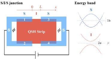
Figure 1: Schematic diagram of the device layout to detect a topological transition. Terminals 1 and 2 (3 and 4) connect to the left (right) superconducting electrodes and the superconducting phase difference between terminals is controlled by a magnetic flux. The band structure of low-energy quasiparticles near the Fermi surface in each region is shown below.

In one approach to realize MKPs, the two opposite edges of a QSHI strip are coupled to superconducting leads with a phase difference of $\pi$ Keselman et al. (2013); Li et al. (2016); Blasi et al. (2019). An experimental signature to detect MKPs in such a Josephson junction is the subharmonic gap structure (SGS); a series of resonant conductance peaks in a voltage-biased Josephson junction. The SGS is generated by multiple Andreev reflections (MAR) when two superconductors are in electric contact and a voltage bias drives sequential Andreev reflections of quasiparticles at the interface between them. Incident quasiparticles gain or lose an energy $eV$ as they travel across the interface, until escaping to the reservoirs for energies above the superconducting gap. In conventional Josephson junctions, the peaks in the SGS come from the singular density of states at the superconducting energy gap edges hosting incident and escaping quasiparticles Lu et al. (2020). The conductance peaks are thus positioned at $eV_{n}\!=\!2\Delta_{0}/n$, with $\Delta_{0}$ the superconducting gap and $n$ an integer number Klapwijk et al. (1982); Octavio et al. (1983); Arnold (1987); Bratus’ et al. (1995); Averin and Bardas (1995); Cuevas et al. (1996). By contrast, due to the presence of Majorana modes in topological Josephson junctions, new resonant channels form in the middle of the energy gap leading to an anomalous SGS with only even integer peaks. That is, the conductance resonances are located at $eV_{m}=2\Delta_{0}/m$ where $m$ is now an even integer Badiane et al. (2011); San-Jose et al. (2013); Zazunov et al. (2016); Setiawan et al. (2017). Anomalous SGSs have been predicted in Josephson junctions mediated by the edge states of a QSHI, which were interpreted as a parity-changing process in a topological Josephson junction Badiane et al. (2011). Angle-resolved SGS have also been explored in two-dimensional Josephson junctions for detecting chiral Majorana states Olde Olthof et al. (2023). However, such setups require breaking time-reversal symmetry by Zeeman coupling from a magnetic material at the QSHI edges, thus hindering their possible experimental implementation.

In this paper we consider a time-reversal invariant QSHI strip with no magnetic elements to simplify these experimental challenges in the search for Majorana states. In our approach, two opposite strip edges are covered by superconductors with a tunable phase difference, see Fig. 1. Importantly, the strip width is such that the edge states are not decoupled. Consequently, the edge states hybridize and their characteristic Dirac-like linear dispersion becomes gapped by $~{}2\alpha$, with $\alpha$ the inter-edge coupling strength. The inter-edge coupling opens a reflection channel between particles at opposite edges, without breaking time-reversal symmetry. The resulting tunnel Josephson junction has variable transmission controlled by $\alpha$. We then consider a bias voltage at terminals 1 and 2 that injects a current collected by terminals 3 and 4 (Fig. 1). At the same time, the phase difference $\phi$ between superconductors can be controlled by a magnetic flux. For $\phi\!=\pi$ the system preserves time-reversal symmetry and hosts MKPs.

Interestingly, the SGS for this junction can be tuned by $\phi$ in stark contrast to conventional Josephson junctions. For $\phi=0$, the junction behavior is in good agreement with conventional BCS Josephson junctions Hurd et al. (1997): the SGS features peaks at $eV_{m}=2\Delta_{L/R}/m$ and $eV_{n}=(\Delta_{L}+\Delta_{R})/n$, with $m$ and $n$ being, respectively, even and odd integers, and $\Delta_{L}$ ($\Delta_{R}$) the left (right) pair potential. As a result, only the even spikes of the SGS split for asymmetric junctions with $\Delta_{L}\neq\Delta_{R}$. By contrast, when time-reversal invariant MKPs emerge for $\phi=\pi$, the junction behavior is very anomalous: only the even resonant peaks ($eV_{m}=2\Delta_{L/R}/m$) appear, and all spikes split for asymmetric junctions. We explain this anomalous behavior by showing that midgap bound states from MKPs are only connected to even order MAR, while odd order processes are only sensitive to the gap edges. Since the emergence of MKPs is associated with an enhanced density of states at zero energy and a reduction of it at the gap edges, only even MAR survive for $\phi=\pi$, while both even and odd conductance peaks appear otherwise. The proposed time-reversal invariant multi-terminal Josephson junction can thus help circumvent some of the experimental challenges in the search for Majorana bound states on QSHI-based superconducting heterostructures.

The rest of the paper is organized as follows. In Section II, we describe the model. We present the transport properties of symmetric and asymmetric junctions in Section III and Section IV, respectively. Finally, we conclude this work with a brief summary in Section V. We also present the tunneling conductance of a normal-superconductor junction and further details of our calculations in the Appendix.

II Model and Formalism.

The low-energy effective edge state Hamiltonian is given by $\mathcal{H=H}_{0}+\mathcal{H}_{S}$ with

$$\mathcal{H}_{0}={} \int dx\hat{\Psi}^{{\dagger}}\left[-i\hbar v\hat{\sigma}_{z}\hat{s}_{z}\partial_{x}+\alpha\hat{\sigma}_{x}-\mu\right]\hat{\Psi},$$ (1)

$$\mathcal{H}_{S}={} \Delta\int dx\left[\hat{\Psi}_{1,\uparrow}^{{\dagger}}\hat{\Psi}_{1,\downarrow}^{{\dagger}}+e^{i\phi}\hat{\Psi}_{-1,\uparrow}^{{\dagger}}\hat{\Psi}_{-1,\downarrow}^{{\dagger}}\right]+\mathrm{h.c.},$$ (2)

and basis $\hat{\Psi}=(\hat{\Psi}_{1,\uparrow}^{{\dagger}},\hat{\Psi}_{1,\downarrow}^{{\dagger}},\hat{\Psi}_{-1,\uparrow}^{{\dagger}},\hat{\Psi}_{-1,\downarrow}^{{\dagger}})^{T}.$ Here, the subscript $\sigma\in\{1,-1\}$ labels the different edges and the Pauli matrices $\hat{\sigma}_{i}$ and $\hat{s}_{i}$, with $i\in\{x,y,z\}$, act on edge and spin spaces, respectively. The chemical potential is $\mu\left(x\right)=\mu\left[\Theta\left(-x\right)+\Theta\left(x-L\right)\right]$, with $\Theta\left(x\right)$ being the Heaviside step function and $L$ the junction length, and $\alpha$ is the coupling strength between opposite edges Zhou et al. (2008). We further assume that the chemical potential for the insulating region $(0<x<L)$ is tuned to the middle of the gap, but remains large ($\mu\gg\alpha$) for the S regions, thus forming a tunnel junction of variable transmission $D=tt^{*}$ with $t=1/\cosh\left(\alpha L/v\right)$. It can be seen that $D$ is tunable by changing the junction length $L$ with a fixed $\alpha$. We define the pair potential $\Delta\left(x\right)=\Delta_{L}\Theta\left(-x\right)+\Delta_{R}\Theta\left(x-L\right)$. Using the Bogoliubov transformation $\hat{\Psi}_{\sigma,s}=\sum_{N}u_{\sigma,s}^{N}\hat{\gamma}_{N}+v_{\sigma,s}^{N,\ast}\hat{\gamma}_{N}^{{\dagger}}$, we derive the Bogoliubov-de Gennes (BdG) Hamiltonian $H=H_{1}\oplus H_{2}$, with

$$H_{\eta=1,2}=\begin{pmatrix}\hat{h}_{i}&\hat{\Delta}_{i}\\ \hat{\Delta}_{i}^{{\dagger}}&-\hat{h}_{i}\end{pmatrix},$$ (3)

and

$$\hat{h}_{1\left(2\right)}={} \begin{pmatrix}\mp i\hbar v\partial_{x}-\mu&\alpha\\ \alpha&\pm i\hbar v\partial_{x}-\mu\end{pmatrix},$$ (4)

$$\hat{\Delta}_{1\left(2\right)}={} \begin{pmatrix}\pm\Delta&0\\ 0&\pm\Delta e^{i\phi}\end{pmatrix},$$ (5)

where $H_{1}$ ($H_{2}$) acts on $(u_{1,\uparrow}^{N},u_{-1,\uparrow}^{N},v_{1,\downarrow}^{N},v_{-1,\downarrow}^{N})^{T}$ [$(u_{1,\downarrow}^{N},u_{-1,\downarrow}^{N},v_{1,\uparrow}^{N},v_{-1,\uparrow}^{N})^{T}$] space. The wavefunctions can be found in Appendix A.

The time-dependent wavefunctions at the central scattering region, (0, $L$), for an incident quasiparticle from terminal 1 read

$$\Phi_{x=0^{-}}=\sum_{n}e^{-i\frac{\left(\epsilon+2neV\right)t}{\hbar}}\begin{pmatrix}{}(J_{\epsilon}^{\left(1\right)}\delta_{n,0}+a_{L,2n}A_{n})\\ B_{n}\\ A_{n}\\ a_{L,2n}e^{-i\phi}B_{n}\end{pmatrix},$$ (6)

$$\Phi_{x=L^{+}}=\sum_{n}e^{-i\frac{\left[\epsilon+\left(2n+1\right)eV\right]t}{\hbar}}\begin{pmatrix}C_{n}\\ a_{R,2n+1}e^{i\phi}D_{n}\\ a_{R,2n+1}C_{n}\\ D_{n}\end{pmatrix},$$ (7)

where $a_{L/R,n}\equiv a_{L/R}\left(\epsilon+neV\right)$ with

$$a_{L/R}\left(\epsilon\right)=\left\{\begin{array}[]{lc}\frac{\epsilon-\text{sgn}\left(\epsilon\right)\left(\epsilon^{2}-\Delta_{L/R}^{2}\right)^{1/2}}{\Delta_{L/R}},&\left|\epsilon\right|>\Delta_{L/R}\\ \frac{\epsilon-i\left(\Delta_{L/R}^{2}-\epsilon^{2}\right)^{1/2}}{\Delta_{L/R}},&\left|\epsilon\right|<\Delta_{L/R}.\end{array},\right.$$ (8)

and $J_{\epsilon}^{\left(1\right)}=\sqrt{1-\left|a_{L}(\epsilon)\right|^{2}}$ being the amplitude of the incident quasiparticle from terminal 1 into the scattering region. The wavefunctions $\Phi_{0^{-}}$ and $\Phi_{L^{+}}$ are connected by the scattering matrices

$$S_{e}=S_{h}^{\ast}=\left[\begin{array}[]{cc}r&t\\ t&-r^{\ast}t/t^{\ast}\end{array}\right],$$ (9)

with $r=-i\tanh\left(\alpha L/v\right)$. Here, we have assumed that $\alpha\gg\Delta_{L/R}$ and thus the scattering matrices can be approximated as energy independent. Consequently, the coefficients $A_{n}$, $B_{n}$, $C_{n}$, and $D_{n}$ are related by

$$\begin{pmatrix}B_{n}\\ C_{n}\end{pmatrix}={} S_{e}\begin{pmatrix}J_{\epsilon}^{\left(1\right)}\delta_{n,0}+a_{L,2n}A_{n}\\ a_{R,2n+1}e^{i\phi}D_{n}\end{pmatrix},$$ (10)

$$\begin{pmatrix}A_{n}\\ D_{n-1}\end{pmatrix}={} S_{h}\begin{pmatrix}a_{L,2n}e^{-i\phi}B_{n}\\ a_{R,2n-1}C_{n-1}\end{pmatrix}.$$ (11)

Solving Eqs. 10 and 11, we obtain the following recurrence relations for $A_{n}$ and $B_{n}$

$$A_{1,n+1}-a_{R,2n+1}a_{L,2n}A_{1,n}=|r|a_{L,2n+2}e^{-i\phi}B_{1,n+1}-|r|a_{R,2n+1}B_{1,n}+a_{R,1}J_{\epsilon}^{(1)}\delta_{n,0},$$ (12)

$$\frac{Da_{L,2n+2}a_{R,2n+1}}{1-a_{R,2n+1}^{2}e^{i\phi}}B_{1,n+1}-\left[\frac{Da_{R,2n+1}^{2}e^{i\phi}}{1-a_{R,2n+1}^{2}e^{i\phi}}+\frac{Da_{L,2n}^{2}e^{-i\phi}}{1-a_{R,2n-1}^{2}e^{i\phi}}-e^{-i\phi}a_{L,2n}^{2}+1\right]B_{1,n}+\frac{Da_{R,2n-1}a_{L,2n}}{1-a_{R,2n-1}^{2}e^{i\phi}}B_{1,n-1}$$

$$=-|r|J_{\epsilon}^{\left(1\right)}\delta_{n,0},$$ (13)

Next, from the continuity equation $\frac{\partial}{\partial t}\hat{\rho}+\partial_{x}\mathcal{\hat{J}}=0$, with $\hat{\rho}=e\sum\nolimits_{\sigma}(\Psi_{\sigma,\uparrow}^{{\dagger}}\Psi_{\sigma,\uparrow}+\Psi_{\sigma,\downarrow}^{{\dagger}}\Psi_{\sigma,\downarrow})$, we define the current operator $\mathcal{\hat{J}}=\sum\nolimits_{\sigma}\frac{ev\sigma}{\hbar}(\Psi_{\sigma,\uparrow}^{{\dagger}}\Psi_{\sigma,\uparrow}-\Psi_{\sigma,\downarrow}^{{\dagger}}\Psi_{\sigma,\downarrow})$. The average electric current in terminal 1, cf. Eq. 6, is defined as

$$I_{1}=\langle\mathcal{\hat{J}}\rangle={} \frac{e}{h}\sum_{k,n}e^{i\frac{2keVt}{\hbar}}\int\nolimits_{-\infty}^{+\infty}\!\!d\epsilon\left[\left(J_{\epsilon}^{\left(1\right)}\delta_{n+k,0}+a_{L,2\left(n+k\right)}^{\ast}A_{1,n+k}^{\ast}\right)\left(J_{\epsilon}^{\left(1\right)}\delta_{n,0}+a_{L,2n}A_{1,n}\right)-B_{1,n+k}^{\ast}B_{1,n}\right]f_{\epsilon}$$

$$+\frac{e}{h}\sum_{k,n}e^{i\frac{2keVt}{\hbar}}\int\nolimits_{-\infty}^{+\infty}\!\!d\epsilon\left[a_{L,2n}a_{L,2\left(n+k\right)}^{\ast}B_{1,n+k}^{\ast}B_{1,n}-A_{1,n+k}^{\ast}A_{1,n}\right]f_{-\epsilon},$$ (14)

where $f_{\epsilon}=(e^{\epsilon/k_{B}T}+1)^{-1}$ is the Fermi-Dirac distribution function. The dc component of the current corresponds to the $k=0$ harmonic in Eq. 14. Similarly, we can obtain the currents for the other terminals, $I_{i=2-4}$, and obtain the total current as $I=\sum_{i}I_{i}$ (see Appendix C). In the numerical calculations, we solved Eq. 13 by choosing an appropriate cut-off value $\left|n\right|=N$, and normalize it in units of $G_{N}\Delta/e$, where $G_{N}$ is the conductance when all electrodes are in the normal state. The differential conductance is thus obtained as $G=\partial I/\partial V$.

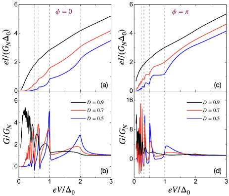
Figure 2: Electric current and differential conductance at temperature $k_{B}T=0.2\Delta_{0}$ as a function of the voltage, for $\phi=0$ (a,b) and $\phi=\pi$ (c,d), for transmissions $D=0.9,0.7,0.5$. In all cases, $\Delta_{L}=\Delta_{R}=\Delta_{0}$. The dashed vertical lines indicate the positions of the resonant spikes.

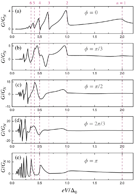
Figure 3: Differential conductance as a function of the voltage at temperature $k_{B}T=0.2\Delta_{0}$ for (a) $\phi=0$, (b) $\phi=\pi/3$, (c) $\phi=\pi/2$, (d) $\phi=2\pi/3$, and (e) $\phi=\pi$. The dashed vertical lines mark the $n$-th order SGS at $2\Delta_{0}/n$ for $n=1,2,3,4,5,6$. In all cases, we choose $\Delta_{L}=\Delta_{R}=\Delta_{0}$ and $D=0.6$.

III Subharmonic gap structure of symmetric junctions

We calculate the current and conductance in Fig. 2 for different junction transmissivity $D=tt^{*}$. We focus on the dc current which experimentally relates to the average electric current in the long time limit. Our formalism can be applied to arbitrary value of $\phi$, but, for clarity, we focus on the time-reversal invariant junction with $\phi=0$ and $\phi=\pi$. In Fig. 2, we consider a symmetric junction with $\Delta_{L}=\Delta_{R}=\Delta_{0}$, and show the current and differential conductance for different values of the transmission. For $\phi=0$, the current characteristic is that of $s$-wave superconductors, where the conductance displays peaks at $eV_{n}=2\Delta_{0}/n$ ($n$ being an integer), see Fig. 2(a,b). By contrast, the SGS becomes $2\Delta_{0}/m$ ($m$ an even integer) for $\phi=\pi$, see Fig. 2(c,d). A SGS with only even resonances was already predicted for time-reversal breaking topological Josephson junctions with zero-energy states Badiane et al. (2011); San-Jose et al. (2013); Zazunov et al. (2016). The exotic SGS can be understood as follows. In the topological superconducting phase, the density of states at the gap edges is suppressed, in contrast to the divergent density for trivial superconductors, see Appendix B. Thus, MAR processes where quasiparticles transmit from the lower gap edge at $-\Delta_{0}$ to the upper one at $\Delta_{0}$ will not necessarily give rise to conductance peaks. By contrast, when the MAR trajectory passes through the midgap MKPs, the resonant channel will boost the MAR transmission and therefore a conductance peak appears. Consequently, the presence of zero-energy states (now MKPs) when $\phi=\pi$ plays an important role in forming the SGS. It is also interesting to compare our results with previous works on phase-tuned MAR in multi-terminal superconductors Lantz et al. (2002); Galaktionov et al. (2012); Riwar et al. (2016); Nowak et al. (2019). In a conventional 3-terminal $s$-wave superconducting interferometer, the phase difference changes the visibility, instead of the shape of the SGS. However, in our setup, the phase difference directly changes the characteristic of the SGS.

To further show how the SGSs evolve with the phase difference, we plot the conductance spectra with equal pair potential $\Delta_{L}=\Delta_{R}=\Delta_{0}$ in Fig. 3. Apart from the previously analyzed cases with $\phi=0$ and $\pi$, the position of the resonant peaks in the SGS is not straightforward to identify. However, it is clear that the odd order resonances gradually disappear by increasing $\phi$ from $0$ to $\pi$. Thus, as the phase reaches $\phi=\pi$, only the even order resonant peaks remain in the SGS.

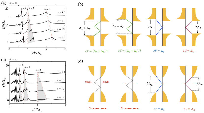
Figure 4: Differential conductance at temperature $k_{B}T=0.2\Delta_{0}$ for $D=0.6$ as the gap ratio $r=\Delta_{L}/\Delta_{R}$ varies for (a) $\phi=0$ and (c) $\phi=\pi$. (b) and (d) show the schematic trajectories of the third-order (first and second panels) and the second-order (third and fourth panels) MAR. For $\phi=0$ (b), both cases result in a conductance peak, since they connect the gap edges with divergent density of states. However, for $\phi=\pi$ (d), the density of states is reduced at the gap edges and the third-order MAR will not generate a conductance peak (gray lines). By contrast, the second-order MAR is assisted by MKPs (red and blue lines) leading to a conductance peak.

IV Asymmetric junctions

Next, we explore the SGS in asymmetric junctions where $\Delta_{L}$ and $\Delta_{R}$ can be different. We focus on the time reversal invariant cases $\phi=0,\pi$ and compare them to the symmetric case. In Fig. 4(a), we consider a trivial junction with $\phi=0$ and change the gap ratio $r=\Delta_{L}/\Delta_{R}$. For $\Delta_{L}\neq\Delta_{R}$, the odd order resonant conductance peaks remain at $eV_{n}=(\Delta_{L}+\Delta_{R})/n$ ($n$ odd), while the even order ones at $eV_{m}=2\Delta_{L/R}/m$ ($m$ even) split into two, see shaded area in Fig. 4(a). To illustrate this difference, we sketch the second ($n=2$) and third ($n=3$) order MAR processes in Fig. 4(b). Since the SGS appears when MAR connect with two band edges, for odd integers (green lines) quasiparticles climb up the same energy $\Delta_{L}+\Delta_{R}$ via MAR. Thus the SGS for $eV_{3}=({\Delta_{L}+\Delta_{R}})/3$ does not split. For even order MAR, however, the two possible paths for quasiparticles gain different energy as indicated by the blue and red lines. Therefore, the second order MAR contribute double peaks at $eV_{n}=\Delta_{L}$ and $eV_{n}=\Delta_{R}$ to the conductance spectra.

Next, we consider the nontrivial case with $\phi=\pi$ and keep the other parameters unchanged. As for symmetric junctions, the odd order MAR resonances disappear [Fig. 4(c)] due to the reduced density of states at the gap edges. As explained above, MAR processes connecting two gap edges only give rise to SGS when a zero-energy state resides in its trajectory. It explains why the odd order gray MAR trajectories sketched in Fig. 4(d) do not contribute to SGS. However, the even order blue and red MAR processes satisfy the resonant condition and thus enhance the onset current leading to the appearance of conductance peaks. This analysis of the SGS is also valid for time-reversal broken topological superconductors.

It is worth highlighting that the different SGSs between $\phi=0$ and $\pi$ are directly connected to the absence or presence, respectively, of zero-energy bound states. Since time-reversal symmetry is preserved in both cases, the emergence of zero-energy bound states should always come in degenerate pairs (MKPs) according to Kramers theorem . In Appendix B, we test such Kramers degeneracy by proposing a different setup configuration with only one superconductor loop. There, we show the correct conductance quantization of $4e^{2}/h$ as corresponds to a pair of spin degenerate Majorana bound states.

V Conclusions

We have studied the charge transport properties of quantum spin Hall strips, with coupled edge states, connected to several superconducting electrodes. Such a setup supports time-reversal invariant Majorana bound states, known as Majorana Kramers pairs, that appear when the phase difference at the Josephson junctions is $\phi=\pi$. We find that the current characteristics strongly change with the phase difference between superconductors at opposite edges. Consequently, the subharmonic gap structure, a sequence of resonant conductance peaks appearing in voltage-biased Josephson junctions due to multiple Andreev processes, is very sensitive to this phase difference. For $\phi=\pi$, due to the presence of zero-energy Majorana Kramers pairs, the odd order multiple Andreev processes do not contribute to the current, and only the even order ones appear in the subharmonic gap structure. Moreover, when the superconductors forming the junction have different gap sizes, all the (even) conductance peaks split, a signature without counterpart in conventional junctions.

We now briefly discuss the feasibility of our experimental proposal to reveal time-reversal invariant Kramers pairs of Majoranas. The most common quantum spin Hall insulator is based on HgTe/CdTe quantum wells, where it has been reported Hart et al. (2014) that the separation between edge channels is reached for $d\sim 400$nm. The coupling strength $\alpha$ between the edge channels with this value of $d$ was estimated to be about $10\mu$eV. The superconducting gap $\Delta$ induced by proximity effect was estimated to be less than $20\mu$eV. In our geometry, we assume a large chemical potential $\mu$, which can be easily satisfied by tuning a top gate Brüne et al. (2012). We also consider $\Delta$ smaller than $\alpha$, which could also be realized by reducing the coupling between the superconducting leads and the quantum spin Hall edges. Our proposal does not require magnetic materials, thus further simplifying its experimental realization, and is highly tunable by an external magnetic flux. Based on these estimations and the recent advances implementing superconducting electrodes on semiconductor quantum wells Hart et al. (2014); Pribiag et al. (2015); Bocquillon et al. (2017); Ren et al. (2019); Fornieri et al. (2019), we are confident that our proposal is within experimental reach.

Acknowledgments. We thank Yukio Tanaka and Fanming Qu for valuable discussions. B. L. acknowledges support from the National Natural Science Foundation of China (project 11904257) and the Natural Science Foundation of Tianjin (project 20JCQNJC01310). P. B. acknowledges support from the Spanish CM “Talento Program” project No. 2019-T1/IND-14088 and the Agencia Estatal de Investigación projects No. PID2020-117992GA-I00 and No. CNS2022-135950.

Appendix A Wavefunctions

In the superconducting side, we can transform the Hamiltonian using the unitary transformation

$$U=\frac{1}{\sqrt{2}}\left[\begin{array}[]{cccc}1&1&0&0\\ 1&-1&0&0\\ 0&0&-1&-1\\ 0&0&-1&1\end{array}\right],$$ (A.1)

and $\tilde{H}_{1\left(2\right)}=UH_{1\left(2\right)}U^{{\dagger}}$ becomes

$$\tilde{H}_{1\left(2\right)}=\left[\begin{array}[]{cccc}-\mu+\alpha&\mp i\partial_{x}&\mp\gamma\xi_{c}\Delta&\mp i\gamma\xi_{s}\Delta\\ \mp i\partial_{x}&-\mu-\alpha&\pm i\gamma\xi_{s}\Delta&\pm\gamma\xi_{c}\Delta\\ \mp\gamma^{\ast}\xi_{c}\Delta&\mp i\gamma^{\ast}\xi_{s}\Delta&\mu-\alpha&\mp i\partial_{x}\\ \pm i\gamma^{\ast}\xi_{s}\Delta&\pm\gamma^{\ast}\xi_{c}\Delta&\mp i\partial_{x}&\mu+\alpha\end{array}\right],$$ (A.2)

with $\xi_{c}=\cos\frac{\phi}{2}$, $\xi_{s}=\sin\frac{\phi}{2}$, and $\gamma=e^{i\frac{\phi}{2}}$. It can be seen that $\alpha$ is negligible in $\tilde{H}_{1\left(2\right)}$ in the limit $\alpha\ll\mu$, and if $\phi\neq 0$ or $\pi$ there are mixed singlet- and triplet-pairings. The wavefunction $\psi$ of $H_{1\left(2\right)}$ can be obtained by $U^{{\dagger}}\tilde{\psi}$, where $\tilde{\psi}$ is the solution of $\tilde{H}_{1\left(2\right)}$. The wavefunctions of $H_{1}$ in the superconducting side are

$$\psi_{1,S}^{e,\rightarrow}=\left[\begin{array}[]{c}u\\ 0\\ v\\ 0\end{array}\right]e^{ikx};\psi_{1,S}^{e,\leftarrow}=\left[\begin{array}[]{c}0\\ u\\ 0\\ ve^{-i\phi}\end{array}\right]e^{-ikx};\psi_{1,S}^{h,\rightarrow}=\left[\begin{array}[]{c}0\\ ve^{i\phi}\\ 0\\ u\end{array}\right]e^{-ikx};\psi_{1,S}^{h,\leftarrow}=\left[\begin{array}[]{c}v\\ 0\\ u\\ 0\end{array}\right]e^{ikx},$$ (A.3)

and the wavefunctions of $H_{2}$ in the superconducting side are

$$\psi_{2,S}^{e,\rightarrow}=\left[\begin{array}[]{c}0\\ u\\ 0\\ -ve^{-i\phi}\end{array}\right]e^{ikx};\psi_{2,S}^{e,\leftarrow}=\left[\begin{array}[]{c}u\\ 0\\ -v\\ 0\end{array}\right]e^{-ikx};\psi_{2,S}^{h,\rightarrow}=\left[\begin{array}[]{c}-v\\ 0\\ u\\ 0\end{array}\right]e^{-ikx};\psi_{2,S}^{h,\leftarrow}=\left[\begin{array}[]{c}0\\ -ve^{i\phi}\\ 0\\ u\end{array}\right]e^{ikx},$$ (A.4)

where $u$ and $v$ are the coherent factors

$$u\left(v\right)=\left[\frac{1}{2}\pm\frac{\sqrt{\epsilon^{2}-\Delta^{2}}}{2\epsilon}\right]^{\frac{1}{2}}.$$ (A.5)

In the central scattering region $0<x<L$, the wavefunctions are given by

$$\psi_{1,c}^{e,1}=\left[\begin{array}[]{c}i\\ 1\\ 0\\ 0\end{array}\right]e^{-\kappa x};\psi_{1,c}^{e,2}=\left[\begin{array}[]{c}-i\\ 1\\ 0\\ 0\end{array}\right]e^{\kappa x};\psi_{1,c}^{h,1}=\left[\begin{array}[]{c}0\\ 0\\ i\\ 1\end{array}\right]e^{-\kappa x};\psi_{1,c}^{h,2}=\left[\begin{array}[]{c}0\\ 0\\ -i\\ 1\end{array}\right]e^{\kappa x},$$ (A.6)

and

$$\psi_{2,c}^{e,1}=\left[\begin{array}[]{c}-i\\ 1\\ 0\\ 0\end{array}\right]e^{-\kappa x};\psi_{2,c}^{e,2}=\left[\begin{array}[]{c}i\\ 1\\ 0\\ 0\end{array}\right]e^{\kappa x};\psi_{2,c}^{h,1}=\left[\begin{array}[]{c}0\\ 0\\ -i\\ 1\end{array}\right]e^{-\kappa x};\psi_{2,c}^{h,2}=\left[\begin{array}[]{c}0\\ 0\\ i\\ 1\end{array}\right]e^{\kappa x},$$ (A.7)

with $\kappa=\alpha/v$.

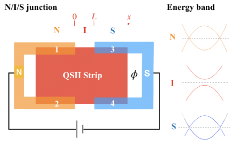
Figure 5: Schematic diagram of the normal-superconductor junction. Terminals 1 and 2 connect to a normal-state injection electrodes, while terminals 3 and 4 connect to superconducting leads. The superconducting phase difference between terminals is controlled by a magnetic flux. Schematic band structures of low-energy quasiparticles near the Fermi surface in each region are shown on the right.

Appendix B Tunneling spectroscopy of a normal-superconductor junction

The emergence of a time-reversal invariant topological superconductor becomes apparent in the tunneling spectroscopy of a junction with superconductors present only on the right region. For $\phi\!=\pi$, the system preserves time-reversal symmetry and can host MKPs. As a result, the zero-bias normal-superconductor conductance is quantized to $4e^{2}/h$.

To show this, we now calculate the differential conductance $dI/dV$ following Ref. Blonder et al., 1982. We define the pair potential $\Delta\left(x\right)=\Delta_{0}\Theta\left(x-L\right)$ for the normal-superconductor junction, see Fig. 5. As a result, the wavefunction for an incident electron from the normal side is

$$\Phi=\sum\nolimits_{\eta=1,2}\left[\psi_{\eta,N}^{e,\rightarrow}+b_{\eta}\psi_{\eta,N}^{e,\leftarrow}+a_{\eta}\psi_{\eta,N}^{h,\leftarrow}\right].$$ (B.1)

The conductance can be obtained as Blonder et al. (1982)

$$G=G_{0}\sum\nolimits_{\eta}\left[1-\left|b_{\eta}\right|^{2}+\left|a_{\eta}\right|^{2}\right],$$ (B.2)

with $G_{0}=e^{2}/h$ being the conductance quantum.

The conductance spectra as a function of phase difference $\phi$ and the bias voltage $eV$ is shown in Fig. 6(a), with transmissivity $D=tt^{*}=0.5$. The subgap resonance peaks vary with $\phi$ and cross at $\phi=\pi$, where the topological phase transition takes place. For $\phi=0$, the conductance reaches the value $G=4e^{2}/h$ at $eV=\pm\Delta_{0}$, see Fig. 6(b), which indicates a perfect Andreev reflection at the gap edges Tanaka and Kashiwaya (1995). Indeed, the conductance for $\phi=0$ behaves like an $s$-wave superconductor where the subgap values reduce by decreasing the transmissivity $D$ Blonder et al. (1982) [Fig. 6(c)]. As expected, these quantized peaks merge at $eV=0$ for $\phi=\pi$ where the MKPs appear, i.e., a single Majorana bound state contributes $2e^{2}/h$ to the conductance. Moreover, the conductance quantization remains robust against $D$ for $\phi=\pi$, exhibiting the celebrated zero-biased conductance peak due to Majorana states Sengupta et al. (2001); Bolech and Demler (2007); Akhmerov et al. (2009); Tanaka et al. (2009); Law et al. (2009); Flensberg (2010); Crépin et al. (2014, 2015); Ikegaya et al. (2015, 2016); Lu et al. (2016); Burset et al. (2017); Keidel et al. (2018); Fleckenstein et al. (2018a, b); Cayao and Burset (2021); Cayao et al. (2022); Lu et al. (2022) [Fig. 6(d)]. At the same time, the $\pi$-difference decreases the local density of states at the gap edges $eV=\pm\Delta_{0}$.

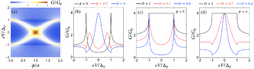
Figure 6: Conductance of a normal-superconductor junction: (a) Contour plot of the conductance $G/G_{0}$, with $G_{0}=e^{2}/h$, as a function of the phase $\phi$ and bias voltage $eV$. The transmissivity is $D=0.5$. Conductance in (a) vs bias voltage for different phase differences $\phi=0$ (black), $\pi/2$ (red), and $\pi$ (blue). (c) Conductance with the phase $\phi=0$ for $D=1$ (black), $0.7$ (red) and $0.5$ (blue). (d) Same as (c) for $\phi=\pi$.

Appendix C Recursive relations and currents in the Josephson junction

In the main text, we have derived the current from injected quasiparticles in terminal 1. We now provide the calculation of currents induced by injection from the other three terminals. The recursive equations for a quasiparticle incident from terminal 2 are

$$A_{2,n+1}-{a}_{R,2n+1}a_{L,2n}A_{2,n}=|r|a_{L,2n+2}e^{i\phi}B_{2,n+1}-|r|{a}_{R,2n+1}B_{2,n}+{a}_{R,1}J_{\epsilon}^{\left(2\right)}\delta_{n0},$$ (C.1)

$$\frac{Da_{L,2n+2}{a}_{R,2n+1}}{1-{a}_{R,2n+1}^{2}e^{-i\phi}}B_{2,n+1}-\left[\frac{D{a}_{R,2n+1}^{2}e^{-i\phi}}{1-{a}_{R,2n+1}^{2}e^{-i\phi}}+\frac{Da_{L,2n}^{2}e^{i\phi}}{1-{a}_{R,2n-1}^{2}e^{-i\phi}}-e^{i\phi}{a}_{L,2n}^{2}+1\right]B_{2,n}+\frac{D{a}_{R,2n-1}a_{L,2n}}{1-{a}_{R,2n-1}^{2}e^{-i\phi}}B_{2,n-1}$$

$$=-|r|J_{\epsilon}^{\left(2\right)}\delta_{n0}.$$ (C.2)

For an incident quasiparticle from terminal 3, the relations are

$$\bar{A}_{3,n+1}-\bar{a}_{L,2n+1}{\bar{a}}_{R,2n}\bar{A}_{3,n}=|r|{{\bar{a}}}_{R,2n+2}e^{i\phi}\bar{B}_{3,n+1}-|r|\bar{a}_{L,2n+1}\bar{B}_{3,n}+\bar{a}_{L,1}J_{\epsilon}^{\left(3\right)}\delta_{n0},$$ (C.3)

$$\frac{D\bar{a}_{L,2n+1}{\bar{a}}_{R,2n+2}}{1-\bar{a}_{L,2n+1}^{2}e^{-i\phi}}\bar{B}_{3,n+1}-\left[\frac{D\bar{a}_{L,2n+1}e^{-i\phi}}{1-\bar{a}_{L,2n+1}^{2}e^{-i\phi}}+\frac{D{\bar{a}}_{R,2n}e^{i\phi}}{1-\bar{a}_{L,2n-1}^{2}e^{-i\phi}}-e^{i\phi}{\bar{a}}_{R,2n}^{2}+1\right]\bar{B}_{3,n}+\frac{D\bar{a}_{L,2n-1}{\bar{a}}_{R,2n}}{1-\bar{a}_{L,2n-1}^{2}e^{-i\phi}}\bar{B}_{3,n-1}$$

$$=-|r|J_{\epsilon}^{\left(3\right)}\delta_{n0}.$$ (C.4)

And for terminal 4, they are

$$\bar{A}_{4,n+1}-\bar{a}_{L,2n+1}{\bar{a}}_{R,2n}\bar{A}_{4,n}=|r|{\bar{a}}_{R,2n+2}e^{-i\phi}\bar{B}_{4,n+1}-|r|\bar{a}_{L,2n+1}\bar{B}_{4,n}+\bar{a}_{L,1}J_{\epsilon}^{\left(4\right)}\delta_{n0},$$ (C.5)

$$\frac{D\bar{a}_{L,2n+1}{\bar{a}}_{R,2n+2}}{1-\bar{a}_{L,2n+1}e^{i\phi}}\bar{B}_{4,n+1}-\left[\frac{D\bar{a}_{L,2n+1}e^{i\phi}}{1-\bar{a}_{L,2n+1}^{2}e^{i\phi}}+\frac{D{\bar{a}}_{R,2n}^{2}e^{-i\phi}}{1-\bar{a}_{L,2n-1}^{2}e^{i\phi}}-{e^{-i\phi}\bar{a}}_{R,2n}^{2}+1\right]\bar{B}_{4,n}+\frac{D\bar{a}_{L,2n-1}{\bar{a}}_{R,2n}}{1-\bar{a}^{2}_{2n-1}e^{i\phi}}\bar{B}_{4,n-1}$$

$$=-|r|J_{\epsilon}^{\left(4\right)}\delta_{n0}.$$ (C.6)

Here, $\bar{a}$ is defined as $\bar{a}_{L/R,n}=a_{L/R}(\epsilon-neV)$. The current sources $J_{\epsilon}^{\left(i\right)}$ are given by $J_{\epsilon}^{\left(2\right)}=\sqrt{1-\left|a_{L}\left(\epsilon\right)\right|^{2}}$ and $J_{\epsilon}^{\left(3\right)}=J_{\epsilon}^{\left(4\right)}=\sqrt{1-\left|a_{R}\left(\epsilon\right)\right|^{2}}$. We have defined ${A}_{n}=A(n,eV)$, ${B}_{n}=B(n,eV)$, $\bar{A}_{n}=A(n,-eV)$ and $\bar{B}_{n}=B(n,-eV)$. The resulting currents $I_{2}$, $I_{3}$, and $I_{4}$ are derived as

$$I_{2}={} \frac{e}{h}\sum\nolimits_{k}e^{i\frac{2keVt}{\hbar}}\int\nolimits_{-\infty}^{+\infty}d\epsilon\sum_{n}\left[\left(J_{\epsilon}^{\left(2\right)}\delta_{n+k,0}+a_{L,2\left(n+k\right)}^{\ast}A_{2,n+k}^{\ast}\right)\left(J_{\epsilon}^{\left(2\right)}\delta_{n,0}+a_{L,2n}A_{2,n}\right)-B_{2,n+k}^{\ast}B_{2,n}\right]f_{\epsilon}$$

$$+\frac{e}{h}\sum\nolimits_{k}e^{i\frac{2keVt}{\hbar}}\int\nolimits_{-\infty}^{+\infty}d\epsilon\sum_{n}\left[a_{L,2n}a_{L,2\left(n+k\right)}^{\ast}B_{2,n+k}^{\ast}B_{2,n}-A_{2,n+k}^{\ast}A_{2,n}\right]f_{-\epsilon},$$ (C.7)

$$I_{3}={} \frac{e}{h}\sum\nolimits_{k}e^{i\frac{2keVt}{\hbar}}\int\nolimits_{-\infty}^{+\infty}d\epsilon\sum_{n}\left[-\left(J_{\epsilon}^{\left(3\right)}\delta_{n+k,0}+\bar{a}_{R,2\left(n+k\right)}^{\ast}\bar{A}_{3,n+k}^{\ast}\right)\left(J_{\epsilon}^{\left(3\right)}\delta_{n,0}+\bar{a}_{R,2n}\bar{A}_{3,n}\right)+\bar{B}_{3,n+k}^{\ast}\bar{B}_{3,n}\right]f_{\epsilon}$$

$$+\frac{e}{h}\sum\nolimits_{k}e^{i\frac{2keVt}{\hbar}}\int\nolimits_{-\infty}^{+\infty}d\epsilon\sum_{n}\left[-\bar{a}_{R,2n}a_{R,2\left(n+k\right)}^{\ast}\bar{B}_{3,n+k}^{\ast}\bar{B}_{3,n}+\bar{A}_{3,n+k}^{\ast}\bar{A}_{3,n}\right]f_{-\epsilon},$$ (C.8)

$$I_{4}={} \frac{e}{h}\sum\nolimits_{k}e^{i\frac{2keVt}{\hbar}}\int\nolimits_{-\infty}^{+\infty}d\epsilon\sum_{n}\left[-\left(J_{\epsilon}^{\left(4\right)}\delta_{n+k,0}+\bar{a}_{R,2\left(n+k\right)}^{\ast}\bar{A}_{4,n+k}^{\ast}\right)\left(J_{\epsilon}^{\left(4\right)}\delta_{n,0}+\bar{a}_{R,2n}\bar{A}_{4,n}\right)+\bar{B}_{4,n+k}^{\ast}\bar{B}_{4,n}\right]f_{\epsilon}$$

$$+\frac{e}{h}\sum\nolimits_{k}e^{i\frac{2keVt}{\hbar}}\int\nolimits_{-\infty}^{+\infty}d\epsilon\sum_{n}\left[-\bar{a}_{R,2n}a_{R,2\left(n+k\right)}^{\ast}\bar{B}_{4,n+k}^{\ast}\bar{B}_{4,n}+\bar{A}_{4,n+k}^{\ast}\bar{A}_{4,n}\right]f_{-\epsilon}.$$ (C.9)

References

- Kane and Mele (2005a) C. L. Kane and E. J. Mele, “Quantum spin hall effect in graphene,” Phys. Rev. Lett. 95, 226801 (2005a).
- Kane and Mele (2005b) C. L. Kane and E. J. Mele, “ topological order and the quantum spin hall effect,” Phys. Rev. Lett. 95, 146802 (2005b).
- Bernevig et al. (2006) B. A. Bernevig, T. L. Hughes, and S. C. Zhang, “Quantum spin Hall effect and topological phase transition in HgTe quantum wells,” Science 314, 1757 (2006).
- Liu et al. (2008) Chaoxing Liu, Taylor L. Hughes, Xiao-Liang Qi, Kang Wang, and Shou-Cheng Zhang, “Quantum spin Hall effect in inverted type-II semiconductors,” Phys. Rev. Lett. 100, 236601 (2008).
- Wu et al. (2006) Congjun Wu, B Andrei Bernevig, and Shou-Cheng Zhang, “Helical Liquid and the Edge of Quantum Spin Hall Systems,” Phys. Rev. Lett. 96, 106401 (2006).
- Xu and Moore (2006) Cenke Xu and J. E. Moore, “Stability of the quantum spin hall effect: Effects of interactions, disorder, and topology,” Phys. Rev. B 73, 045322 (2006).
- Roth et al. (2010) Andreas Roth, Christoph Brüne, Hartmut Buhmann, Laurens W. Molenkamp, Joseph Maciejko, Xiao-Liang Qi, and Shou-Cheng Zhang, “Nonlocal Transport in the Quantum Spin Hall State,” Science 325, 294–297 (2010).
- Brüne et al. (2012) Christoph Brüne, Andreas Roth, Hartmut Buhmann, Ewelina M. Hankiewicz, Laurens W. Molenkamp, Joseph Maciejko, Xiao-Liang Qi, and Shou-Cheng Zhang, “Spin polarization of the quantum spin Hall edge states,” Nat. Phys. 8, 485–490 (2012).
- Hsu et al. (2021) Chen-Hsuan Hsu, Peter Stano, Jelena Klinovaja, and Daniel Loss, “Helical liquids in semiconductors,” Semicond. Sci. Tech. 36, 123003 (2021).
- Kitaev (2001) A Kitaev, “Unpaired majorana fermions in quantum wires,” PHYS-USP+ 44, 131–136 (2001).
- Kitaev (2003) A. Kitaev, “Fault-tolerant quantum computation by anyons,” Ann Phys (N Y) 303, 2 (2003).
- Nayak et al. (2008) Chetan Nayak, Steven H. Simon, Ady Stern, Michael Freedman, and Sankar Das Sarma, “Non-abelian anyons and topological quantum computation,” Rev. Mod. Phys. 80, 1083–1159 (2008).
- Hasan and Kane (2010) M. Z. Hasan and C. L. Kane, “Colloquium: Topological insulators,” Rev. Mod. Phys. 82, 3045–3067 (2010).
- Qi and Zhang (2011) Xiao-Liang Qi and Shou-Cheng Zhang, “Topological insulators and superconductors,” Rev. Mod. Phys. 83, 1057–1110 (2011).
- Alicea et al. (2011) Jason Alicea, Yuval Oreg, Gil Refael, Felix von Oppen, and Matthew P. A. Fisher, “Non-abelian statistics and topological quantum information processing in 1d wire networks,” Nat. Phys. 7, 412–417 (2011).
- Leijnse and Flensberg (2012) Martin Leijnse and Karsten Flensberg, “Introduction to topological superconductivity and majorana fermions,” Semicond. Sci. Technol. 27, 124003 (2012).
- Ando (2013) Yoichi Ando, “Topological insulator materials,” J. Phys. Soc. Jpn. 82, 102001 (2013).
- Tkachov and Hankiewicz (2013) G. Tkachov and E. M. Hankiewicz, “Spin-helical transport in normal and superconducting topological insulators,” Phys. Status Solidi B 250, 215–232 (2013).
- Kwon et al. (2004) H.-J. Kwon, K. Sengupta, and V. M. Yakovenko, “Fractional ac josephson effect in p- and d-wave superconductors,” Eur. Phys. J. B 37, 349–361 (2004).
- Fu and Kane (2008) Liang Fu and C. L. Kane, “Superconducting proximity effect and majorana fermions at the surface of a topological insulator,” Phys. Rev. Lett. 100, 096407 (2008).
- Fu and Kane (2009) Liang Fu and C. L. Kane, “Josephson current and noise at a superconductor/quantum-spin-hall-insulator/superconductor junction,” Phys. Rev. B 79, 161408 (2009).
- Note (1) Kramers theorem states that, in a time-reversal symmetric system with half-integer total spin, for any energy eigenstate its time-reversal state is also an eigenstate with the same energy.
- Kim et al. (2016) Younghyun Kim, Dong E. Liu, Erikas Gaidamauskas, Jens Paaske, Karsten Flensberg, and Roman M. Lutchyn, “Signatures of majorana kramers pairs in superconductor-luttinger liquid and superconductor-quantum dot-normal lead junctions,” Phys. Rev. B 94, 075439 (2016).
- Zhang et al. (2013) Fan Zhang, C. L. Kane, and E. J. Mele, “Time-reversal-invariant topological superconductivity and majorana kramers pairs,” Phys. Rev. Lett. 111, 056402 (2013).
- Keselman et al. (2013) Anna Keselman, Liang Fu, Ady Stern, and Erez Berg, “Inducing time-reversal-invariant topological superconductivity and fermion parity pumping in quantum wires,” Phys. Rev. Lett. 111, 116402 (2013).
- Li et al. (2016) Jian Li, Wei Pan, B. Andrei Bernevig, and Roman M. Lutchyn, “Detection of majorana kramers pairs using a quantum point contact,” Phys. Rev. Lett. 117, 046804 (2016).
- Blasi et al. (2019) Gianmichele Blasi, Fabio Taddei, Vittorio Giovannetti, and Alessandro Braggio, “Manipulation of cooper pair entanglement in hybrid topological josephson junctions,” Phys. Rev. B 99, 064514 (2019).
- Lu et al. (2020) Bo Lu, Pablo Burset, and Yukio Tanaka, “Spin-polarized multiple andreev reflections in spin-split superconductors,” Phys. Rev. B 101, 020502 (2020).
- Klapwijk et al. (1982) T.M. Klapwijk, G.E. Blonder, and M. Tinkham, “Explanation of subharmonic energy gap structure in superconducting contacts,” Physica B+C 109-110, 1657–1664 (1982), 16th International Conference on Low Temperature Physics, Part 3.
- Octavio et al. (1983) M. Octavio, M. Tinkham, G. E. Blonder, and T. M. Klapwijk, “Subharmonic energy-gap structure in superconducting constrictions,” Phys. Rev. B 27, 6739–6746 (1983).
- Arnold (1987) Gerald B. Arnold, “Superconducting tunneling without the tunneling hamiltonian. ii. subgap harmonic structure,” J. Low. Temp. Phys. 68, 1–27 (1987).
- Bratus’ et al. (1995) E. N. Bratus’, V. S. Shumeiko, and G. Wendin, “Theory of subharmonic gap structure in superconducting mesoscopic tunnel contacts,” Phys. Rev. Lett. 74, 2110–2113 (1995).
- Averin and Bardas (1995) D. Averin and A. Bardas, “ac josephson effect in a single quantum channel,” Phys. Rev. Lett. 75, 1831–1834 (1995).
- Cuevas et al. (1996) J. C. Cuevas, A. Martín-Rodero, and A. Levy Yeyati, “Hamiltonian approach to the transport properties of superconducting quantum point contacts,” Phys. Rev. B 54, 7366–7379 (1996).
- Badiane et al. (2011) Driss M. Badiane, Manuel Houzet, and Julia S. Meyer, “Nonequilibrium josephson effect through helical edge states,” Phys. Rev. Lett. 107, 177002 (2011).
- San-Jose et al. (2013) Pablo San-Jose, Jorge Cayao, Elsa Prada, and Ramón Aguado, “Multiple andreev reflection and critical current in topological superconducting nanowire junctions,” New J. Phys. 15, 075019 (2013).
- Zazunov et al. (2016) A. Zazunov, R. Egger, and A. Levy Yeyati, “Low-energy theory of transport in majorana wire junctions,” Phys. Rev. B 94, 014502 (2016).
- Setiawan et al. (2017) F. Setiawan, William S. Cole, Jay D. Sau, and S. Das Sarma, “Transport in superconductor–normal metal–superconductor tunneling structures: Spinful -wave and spin-orbit-coupled topological wires,” Phys. Rev. B 95, 174515 (2017).
- Olde Olthof et al. (2023) Linde A. B. Olde Olthof, Stijn R. de Wit, Shu-Ichiro Suzuki, Inanc Adagideli, Jason W. A. Robinson, and Alexander Brinkman, “Multiple andreev reflections in topological josephson junctions with chiral majorana modes,” Phys. Rev. B 107, 184510 (2023).
- Hurd et al. (1997) Magnus Hurd, Supriyo Datta, and Philip F. Bagwell, “ac josephson effect for asymmetric superconducting junctions,” Phys. Rev. B 56, 11232–11245 (1997).
- Zhou et al. (2008) Bin Zhou, Hai-Zhou Lu, Rui-Lin Chu, Shun-Qing Shen, and Qian Niu, “Finite size effects on helical edge states in a quantum spin-hall system,” Phys. Rev. Lett. 101, 246807 (2008).
- Lantz et al. (2002) J. Lantz, V. S. Shumeiko, E. Bratus, and G. Wendin, “Phase-dependent multiple andreev reflections in sns interferometers,” Phys. Rev. B 65, 134523 (2002).
- Galaktionov et al. (2012) Artem V. Galaktionov, Andrei D. Zaikin, and Leonid S. Kuzmin, “Andreev interferometer with three superconducting electrodes,” Phys. Rev. B 85, 224523 (2012).
- Riwar et al. (2016) Roman-Pascal Riwar, Driss M. Badiane, Manuel Houzet, Julia S. Meyer, and Yuli V. Nazarov, “Cross-correlations of coherent multiple andreev reflections,” Physica E 76, 231–237 (2016).
- Nowak et al. (2019) M. P. Nowak, M. Wimmer, and A. R. Akhmerov, “Supercurrent carried by nonequilibrium quasiparticles in a multiterminal josephson junction,” Phys. Rev. B 99, 075416 (2019).
- Hart et al. (2014) Sean Hart, Hechen Ren, Timo Wagner, Philipp Leubner, Mathias Mühlbauer, Christoph Brüne, Hartmut Buhmann, Laurens W. Molenkamp, and Amir Yacoby, “Induced superconductivity in the quantum spin Hall edge,” Nat. Phys. 10, 638–643 (2014).
- Pribiag et al. (2015) Vlad S. Pribiag, Arjan J. A. Beukman, Fanming Qu, Maja C. Cassidy, Christophe Charpentier, Werner Wegscheider, and Leo P. Kouwenhoven, “Edge-mode superconductivity in a two-dimensional topological insulator,” Nat. Nanotechnol. 10, 593–597 (2015).
- Bocquillon et al. (2017) Erwann Bocquillon, Russell S. Deacon, Jonas Wiedenmann, Philipp Leubner, Teunis M. Klapwijk, Christoph Brüne, Koji Ishibashi, Hartmut Buhmann, and Laurens W. Molenkamp, “Gapless Andreev bound states in the quantum spin Hall insulator HgTe,” Nat. Nanotechnol. 12, 137–143 (2017).
- Ren et al. (2019) Hechen Ren, Falko Pientka, Sean Hart, Andrew T. Pierce, Michael Kosowsky, Lukas Lunczer, Raimund Schlereth, Benedikt Scharf, Ewelina M. Hankiewicz, Laurens W. Molenkamp, Bertrand I. Halperin, and Amir Yacoby, “Topological superconductivity in a phase-controlled josephson junction,” Nature 569, 93–98 (2019).
- Fornieri et al. (2019) Antonio Fornieri, Alexander M. Whiticar, F. Setiawan, Elías Portolés, Asbjørn C. C. Drachmann, Anna Keselman, Sergei Gronin, Candice Thomas, Tian Wang, Ray Kallaher, Geoffrey C. Gardner, Erez Berg, Michael J. Manfra, Ady Stern, Charles M. Marcus, and Fabrizio Nichele, “Evidence of topological superconductivity in planar josephson junctions,” Nature 569, 89–92 (2019).
- Blonder et al. (1982) G. E. Blonder, M. Tinkham, and T. M. Klapwijk, “Transition from metallic to tunneling regimes in superconducting microconstrictions: Excess current, charge imbalance, and supercurrent conversion,” Phys. Rev. B 25, 4515–4532 (1982).
- Tanaka and Kashiwaya (1995) Yukio Tanaka and Satoshi Kashiwaya, “Theory of tunneling spectroscopy of -wave superconductors,” Phys. Rev. Lett. 74, 3451–3454 (1995).
- Sengupta et al. (2001) K. Sengupta, Igor Žutić, Hyok-Jon Kwon, Victor M. Yakovenko, and S. Das Sarma, “Midgap edge states and pairing symmetry of quasi-one-dimensional organic superconductors,” Phys. Rev. B 63, 144531 (2001).
- Bolech and Demler (2007) C. J. Bolech and Eugene Demler, “Observing majorana bound states in -wave superconductors using noise measurements in tunneling experiments,” Phys. Rev. Lett. 98, 237002 (2007).
- Akhmerov et al. (2009) A. R. Akhmerov, Johan Nilsson, and C. W. J. Beenakker, “Electrically detected interferometry of majorana fermions in a topological insulator,” Phys. Rev. Lett. 102, 216404 (2009).
- Tanaka et al. (2009) Yukio Tanaka, Takehito Yokoyama, and Naoto Nagaosa, “Manipulation of the majorana fermion, andreev reflection, and josephson current on topological insulators,” Phys. Rev. Lett. 103, 107002 (2009).
- Law et al. (2009) K. T. Law, Patrick A. Lee, and T. K. Ng, “Majorana fermion induced resonant andreev reflection,” Phys. Rev. Lett. 103, 237001 (2009).
- Flensberg (2010) Karsten Flensberg, “Tunneling characteristics of a chain of majorana bound states,” Phys. Rev. B 82, 180516 (2010).
- Crépin et al. (2014) François Crépin, Björn Trauzettel, and Fabrizio Dolcini, “Signatures of Majorana bound states in transport properties of hybrid structures based on helical liquids,” Phys. Rev. B 89, 205115 (2014).
- Crépin et al. (2015) François Crépin, Pablo Burset, and Björn Trauzettel, “Odd-frequency triplet superconductivity at the helical edge of a topological insulator,” Phys. Rev. B 92, 100507(R) (2015).
- Ikegaya et al. (2015) Satoshi Ikegaya, Yasuhiro Asano, and Yukio Tanaka, “Anomalous proximity effect and theoretical design for its realization,” Phys. Rev. B 91, 174511 (2015).
- Ikegaya et al. (2016) Satoshi Ikegaya, Shu-Ichiro Suzuki, Yukio Tanaka, and Yasuhiro Asano, “Quantization of conductance minimum and index theorem,” Phys. Rev. B 94, 054512 (2016).
- Lu et al. (2016) Bo Lu, Pablo Burset, Yasunari Tanuma, Alexander A. Golubov, Yasuhiro Asano, and Yukio Tanaka, “Influence of the impurity scattering on charge transport in unconventional superconductor junctions,” Phys. Rev. B 94, 014504 (2016).
- Burset et al. (2017) Pablo Burset, Bo Lu, Shun Tamura, and Yukio Tanaka, “Current fluctuations in unconventional superconductor junctions with impurity scattering,” Phys. Rev. B 95, 224502 (2017).
- Keidel et al. (2018) Felix Keidel, Pablo Burset, and Björn Trauzettel, “Tunable hybridization of majorana bound states at the quantum spin hall edge,” Phys. Rev. B 97, 075408 (2018).
- Fleckenstein et al. (2018a) Christoph Fleckenstein, Felix Keidel, Björn Trauzettel, and Niccoló Traverso Ziani, “The invisible majorana bound state at the helical edge,” Eur. Phys. J-spec. Top. 227, 1377–1386 (2018a).
- Fleckenstein et al. (2018b) C. Fleckenstein, N. Traverso Ziani, and B. Trauzettel, “Conductance signatures of odd-frequency superconductivity in quantum spin Hall systems using a quantum point contact,” Phys. Rev. B 97, 134523 (2018b).
- Cayao and Burset (2021) Jorge Cayao and Pablo Burset, “Confinement-induced zero-bias peaks in conventional superconductor hybrids,” Phys. Rev. B 104, 134507 (2021).
- Cayao et al. (2022) Jorge Cayao, Paramita Dutta, Pablo Burset, and Annica M. Black-Schaffer, “Phase-tunable electron transport assisted by odd-frequency cooper pairs in topological josephson junctions,” Phys. Rev. B 106, L100502 (2022).
- Lu et al. (2022) Bo Lu, Guanxin Cheng, Pablo Burset, and Yukio Tanaka, “Identifying majorana bound states at quantum spin hall edges using a metallic probe,” Phys. Rev. B 106, 245427 (2022).