Ti-MAE: Self-Supervised Masked Time Series Autoencoders

Abstract

Multivariate Time Series forecasting has been an increasingly popular topic in various applications and scenarios. Recently, contrastive learning and Transformer-based models have achieved good performance in many long-term series forecasting tasks. However, there are still several issues in existing methods. First, the training paradigm of contrastive learning and downstream prediction tasks are inconsistent, leading to inaccurate prediction results. Second, existing Transformer-based models which resort to similar patterns in historical time series data for predicting future values generally induce severe distribution shift problems, and do not fully leverage the sequence information compared to self-supervised methods. To address these issues, we propose a novel framework named Ti-MAE, in which the input time series are assumed to follow an integrate distribution. In detail, Ti-MAE randomly masks out embedded time series data and learns an autoencoder to reconstruct them at the point-level. Ti-MAE adopts mask modeling (rather than contrastive learning) as the auxiliary task and bridges the connection between existing representation learning and generative Transformer-based methods, reducing the difference between upstream and downstream forecasting tasks while maintaining the utilization of original time series data. Experiments on several public real-world datasets demonstrate that our framework of masked autoencoding could learn strong representations directly from the raw data, yielding better performance in time series forecasting and classification tasks.

1 Introduction

Time series modeling has an urgent need in many fields, such as time series classification (Dau et al., 2019), demand forecasting (Carbonneau et al., 2008), and anomaly detection (Laptev et al., 2017). Recently, long sequence time series forecasting (LSTF), which aims to predict the change of values in a long future period, has aroused significant interests of researchers. In the previous work, most of the self-supervised representation learning methods on time series aim to learn transformation-invariant features via contrastive learning to be applied on downstream tasks. Although these methods perform well on classification tasks, there is still a gap between their performance and other supervised models on forecasting tasks. Apart from the inevitable distortion to time series caused by augmentation strategies they have borrowed from vision or language, the inconsistency between upstream contrastive learning approaches and downstream forecasting tasks should be also a major cause of this problem. Besides, as the latest contrastive learning frameworks (Yue et al., 2022; Woo et al., 2022a) reported, Transformer (Vaswani et al., 2017) performs worse than CNN-based backbones, which is also not consistent with our experience. We have to reveal the differences and relationships between existing contrastive learning and supervised methods on time series.

As an alternative of contrastive learning, denoising autoencoders (Vincent et al., 2008) are also used to be an auxiliary task to learn intermediate representation from the data. Due to the ability of Transformer to capture long-range dependencies, many of existing methods (Zhou et al., 2021; Wu et al., 2021; Woo et al., 2022b) focused on reducing the time complexity and memory usage caused by vanilla attention mechanism such as sparse attention or correlation to process longer time series. These transformer-based models all follow the same training paradigm as Figure 1(a) shows, which learns similar patterns from input historical time series segments and predict future time series values from captured patterns. These so-called generative Transformer-based models are actually a special kind of denoising autoencoders, where we only mask the future values and reconstruct them.

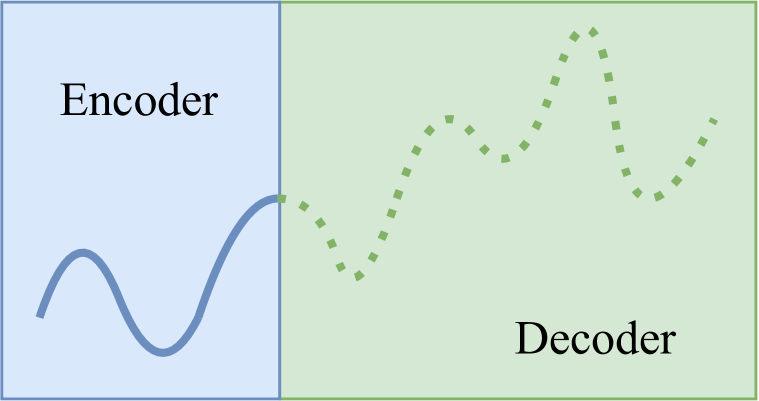
(a) End-to-end forecasting.

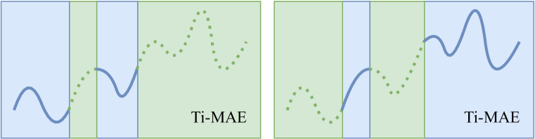
(b) Random masking applied in Ti-MAE.

Figure 1: Different masking strategies in generative Transformer-based models on time series, where blue areas signify the sequence fed into the encoder and green areas means the sequence to be generated. Left: The training paradigm of existing Transformer-based forecasting models, which can be seen as a special continuous masking strategy (only masks future time series and reconstructs them). Right: Random masking strategy applied in Ti-MAE, which can produce different views fed into the encoder in each iteration, fully leveraging the whole input time series.

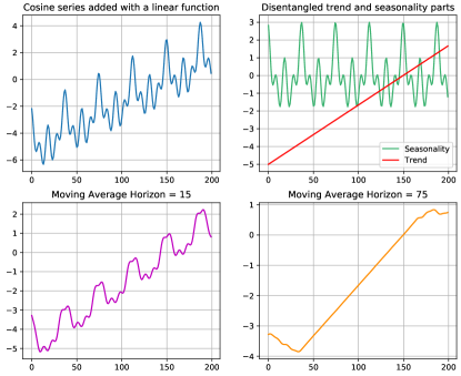
Figure 2: Example of disentanglement. Top Left: Simulated input cosine series added with a linear trend. Top Right: The true trend and seasonality parts of the input. Bottom Left: Disentangled trend part though average pooling with the sliding window size of 15. Bottom Right: Disentangled trend part though average pooling with the sliding window size of 75.

However, this continuous masking strategy is usually accompanied by two severe problems. For one thing, continuous masking strategy will limit the learning ability of the model, which captures only the information of the visible sequence and some mapping relationship between the historical and the future segments. Similar problems have been reported in vision tasks (Zhang et al., 2017). For another, continuous masking strategy will induce severe distribution shift problems, especially when the prediction horizon is longer than input sequence. In reality, most of the time series data collected from real scenarios are non-stationary, whose mean or variance changes over time. Similar problems were also observed in previous studies (Qiu et al., 2018; Oreshkin et al., 2020; Wu et al., 2021; Woo et al., 2022a). Most of them have tried to disentangle the input time series into a trend part and a seasonality part in order to enhance the capture of periodic features and to make the model robust to outlier noises. Specifically, they utilize moving average implemented by one average pooling layer with a fixed size sliding window to gain trend information of input time series. Then they capture seasonality features from periodic sequences, which are obtained by simply subtracting trend items from the original signal. To further clarify the mechanism of this disentanglement, we intuitively propose an easy but comprehensible description of disentangled time series as

$$\bm{y}(t) =\textit{Trend}(t)+\textit{Seasonality}(t)+\mathrm{Noises}.$$ (1)

For better illustration, we simply use polynomial series $\sum_{n}t^{n}$ and Fourier cosine series $\sum_{n}\cos^{n}t$ to respectively describe trend parts and seasonality parts of the original time series in Eq.(1). Apparently, the seasonality part is stationary when we set a proper observation horizon (not less than the maximum period of seasonality parts), while the moments of the trend part change continuously over time. Figure 2 illustrates that the size of sliding window in average pooling layer plays a vital role in the quality of disentangled trend part. Natural time series data generally have more complex periodic patterns, which means we have to employ longer sliding windows or other hierarchical disposals. In addition, when moving average is used to capture the trend parts, both ends of a sequence need to be padded for alignment, which causes inevitable data distortion at the head and tail. These observed phenomenons suggest there are still some unresolved issues in the current disentanglement.

To address these issues, this paper proposes a novel Transformer-based framework named Ti-MAE as shown in Figure 3. Ti-MAE randomly masks out parts of embedded time series data and learns an autoencoder to reconstruct them at the point-level in the training stage. Figure 1 shows the difference between random masking and fixed continuous masking in end-to-end models, where we adequately leverage all the input sequence with different combination of visible tokens. Random masking takes the overall distribution of inputs into consideration, which can therefore alleviate the distribution shift problem. Moreover, with the power of pre-training or representation learning embodied in the encoder-decoder structure, Ti-MAE provides a universal scheme for both forecasting and classification. The contributions of our work are summarized as follows:

• We provide a novel perspective to bridge the connection between existing contrastive learning and generative Transformer-based models on time series and point out the inconsistency and deficiencies of them on downstream tasks.

• We propose Ti-MAE, a masked time series autoencoders which can learn strong representations with less inductive bias or hierarchical trick. Masking time series modeling in training stage adequately leverages the input data and successfully alleviates the distribution shift problem. Due to the flexible setting of masking ratio, Ti-MAE can adapt to complex scenarios which require the trained model to make forecasting simultaneously for multiple time windows with various sizes without re-training.

• Ti-MAE has achieved excellent performance for both forecasting and classification tasks on several public real-world time series datasets, demonstrating the power of pre-training or representation learning of Ti-MAE in the time series domain.

2 Related Work

2.1 Transformer-based time series model

Due to the ability of Transformer to capture long-range dependencies, Transformer-based model has been widely used in language and vision tasks. Song et al. (2018); Ma et al. (2019); LI et al. (2019) tried to directly apply vanilla Transformer to time series data but failed in long sequence time series forecasting tasks as self-attention operation scales quadratically with the input sequence length. Child et al. (2019); Zhou et al. (2021); Liu et al. (2022) noticed the long tail distribution in self-attention feature map so that they utilized sparse attention mechanism to reduce time complexity and memory usage of vanilla Transformer for processing longer sequences. Unfortunately, applying too long input sequence in training stage will degrade the forecasting accuracy of the model (Wu et al., 2021), which is in contrast to the ability that Transformer-based model can capture long-range dependencies. Some of the latest works like ETSformer (Woo et al., 2022b) and FEDformer (Zhou et al., 2022) also rely heavily on disentanglement and extra introduced domain knowledge.

2.2 Time Series Representation Learning

Self-supervised representation learning has achieved good performance in time series domain, especially using contrastive learning to learn a good intermediate representation. Lei et al. (2019); Franceschi et al. (2019) used loss function of metric learning to preserve pairwise similarities in the time domain. CPC (van den Oord et al., 2018) first proposed contrastive predictive coding and InfoNCE, which treats the data from the same sequence as positive pairs while the different noise data from the mini-batch as negative pairs. Different data augmentations on time series data were proposed to capture transformation-invariant features at semantic level (Eldele et al., 2021; Yue et al., 2022). CoST (Woo et al., 2022a) introduced extra inductive biases in frequency domain through DFT and separately processed disentangled trend and seasonality parts of the original time series data to encourage discriminative seasonal and trend representations. Almost all of these methods rely on heavily data augmentation or other domain knowledge like hierarchy and disentanglement.

2.3 Masked Data Modeling

Masked language modeling is a widely adapted method for pre-training in NLP. BERT (Devlin et al., 2019) holds out a portion of the input sequence and predicts the missing content in training stage, which can generate good representations to various downstream tasks. Masked image encoding methods are also used for learning image representations. Pathak et al. (2016) recovered a small portion of missing regions using convolution. Motivated by the huge successes in NLP, recent methods (Bao et al., 2021; Dosovitskiy et al., 2021) are resort to Transformers to predict unknown pixels. MAE (He et al., 2021) proposed to mask a high portion of patches and retain a small set of visible patches received by encoder in pre-training on image data. Zerveas et al. (2021) directly masked a small portion of time series to learn representations. Pang et al. (2022); Tong et al. (2022); Feichtenhofer et al. (2022) have shown that MAE-style methods are effective to learn good representations. Specially designed for enhancing the performance of spatial-temporal graph neural networks, TSformer (Shao et al., 2022) concurrently tried to use MAE to generate intermediate representations for spatial-temporal data. In addition, ExtraMAE (fang Zha, 2022) used RNN as the backbone with the masking scheme for fast time series generation. Different from these methods, Ti-MAE inherits the advantages of Transformer in modeling long time dependencies, and develops a universal time series generation method for both forecasting and classification, with outstanding performance in comparison with state-of-the-art transformer time series models and contrastive learning methods.

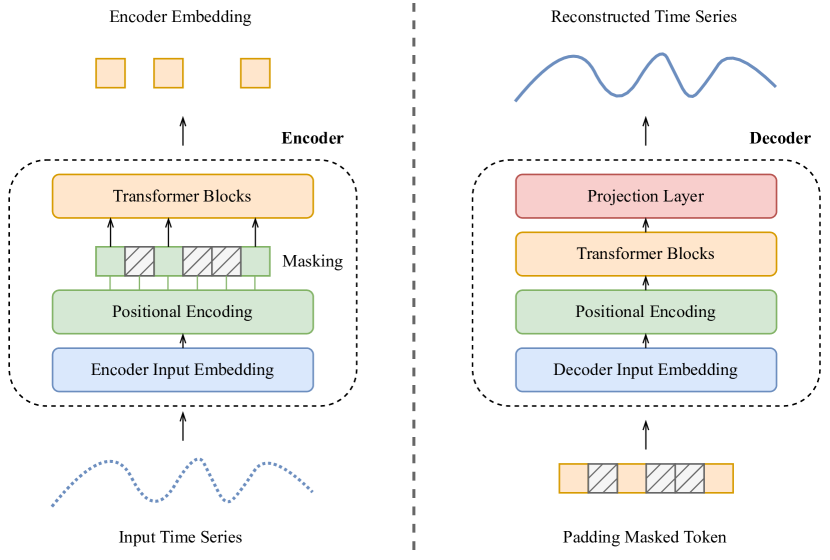
Figure 3: Ti-MAE structure overview. Left: The encoder receives raw time series inputs. After embedding inputs into tokens on timestamp, we randomly mask a large subset of tokens. Then we feed all the visible tokens into Transformer blocks to capture dependencies. Right: The lighter decoder processes encoded tokens padded with masked tokens and reconstructs the original time series at the point-level.

3 Methodology

3.1 Problem Definition

Let $\mathcal{X}=(\bm{x}_{1},\bm{x}_{2},\dots,\bm{x}_{T})\in\mathbb{R}^{T\times m}$ be a multivariate time series instance with length of $T$ , where $m$ is the dimension of each signal. Given a historical multivariate time series segment $\mathcal{X}_{h}\in\mathbb{R}^{h\times m}$ with length of $h$, forecasting tasks aim to predict the next $k$ steps values of $\mathcal{X}_{f}\in\mathbb{R}^{k\times n}$ where $n\leq m$. For classification tasks, we should match the categorical ground truth from a set of labels $\mathcal{C}$ and each time series instance $\mathcal{X}$.

3.2 Model Architecture

The overall architecture of Ti-MAE is shown in Figure 3. Similar as all autoencoders, our framework has an encoder that maps the observed time series signal $\mathcal{X}\in\mathbb{R}^{T\times m}$ to a latent representation $\mathcal{H}\in\mathbb{R}^{T\times n}$, and a decoder that reconstructs the original sequence from the embedding of the encoder on timestamp. Motivated by the great success of other MAE-style approaches (He et al., 2021; Feichtenhofer et al., 2022; Hou et al., 2022), we also adopt an asymmetric design that the encoder only operates visible tokens after applying masking on input embedding, and a lighter decoder processes encoded tokens padded with masked tokens and reconstructs the original time series at the point-level. More details of each component are introduced as follows.

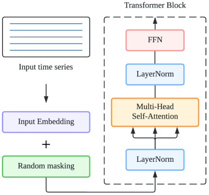
Figure 4: Ti-MAE encoder overview. Left: Encoder input embedding. Right: Details of one Transformer block used in both Ti-MAE encoder and decoder, where we utilize pre-norm instead of post-norm scheme.

Input embedding. Unlike other time series modeling methods, we have not adopted any multi-scale or complex convolution scheme like dilated convolution. Given a time series segment, we directly use one 1-D convolutional layer to extract local temporal features on timestamp across channels. Fixed sinusoidal positional embeddings are added to maintain the position information. Be different from other temporal data embedding approaches, we do not add any handcrafting task-specific or date-specific embeddings so as to introduce as little inductive bias as possible.

Masking. After tokenizing original temporal data into tokens on timestamp, we randomly sample a subset of tokens without replacement which follows the uniform distribution and mask the remaining parts. It is hypothesized and summarized in (He et al., 2021; Feichtenhofer et al., 2022) that the masking ratio is related to the information density and redundancy of the data, which has an immense impact on the performance of the autoencoders. Generally speaking, natural language has higher information density due to its highly discrete word distribution, while images are of heavy spatial redundancy. Specifically, single pixel in one image has lower semantic information so that we can reconstruct a missing region from neighboring pixels by interpolation with little understanding of contents. Thus, data with lower information density should be applied a higher masking ratio to largely eliminate redundancy and prevent the model from focusing only on low-level semantic information. As a benchmark model often used in natural language, BERT (Devlin et al., 2019) uses a masking ratio of 15% while MAE uses a ratio of 75% for images (He et al., 2021) and 90% for videos (Feichtenhofer et al., 2022). Similar as images, time series data also have local continuity so that we should determine a high masking ratio in training stage. The optimal masking ratio of multivariate time series we observe is also around 75%.

Ti-MAE Encoder. Our encoder is a set of vanilla Transformer blocks with input embedding but utilizes pre-norm instead of post-norm in each block, which is shown as Figure 4. Like other MAE-style methods, Ti-MAE’s encoder is applied only on visible tokens after embedding and random masking. This design significantly reduces time complexity and memory usage compared to full encoding.

Ti-MAE Decoder. Our decoder also contains a set of vanilla Transformer blocks applied on the union of the encoded visible tokens and learnable randomly initialized mask tokens. Following (He et al., 2021), the decoder is designed to be smaller than the encoder. Notably, we add positional embeddings to all tokens after padding to supplement the location information of the missing parts. The last layer of the decoder is a linear projection layer which reconstructs the input by predicting all the values at the point-level. The training loss function is the mean squared error (MSE) between the original time series data and the prediction over masking regions.

The encoder and decoder of Ti-MAE are both agnostic to the sequential data with as less domain knowledge as possible. There is no date-specific embedding, hierarchy or disentanglement in contrast to other architectures (Zhou et al., 2021; Wu et al., 2021; Yue et al., 2022; Woo et al., 2022a). Compared to masked autoencoders used in vision tasks, a lot of parameter settings of Ti-MAE have been adjusted to better fit the time series data. We keep the point-level modeling rather than patch embedding for the consistency between masked modeling and downstream forecasting tasks. Unlike (Shao et al., 2022), we directly generate future values from the decoder as prediction, maintaining the consistency of training and inference stages.

4 Experiments

4.1 Experimental Setup

Datasets. We conduct extensively experiments on several public real-world datasets, covering time series forecasting and classification applications. (1) ETT (Electricity Transformer Temperature) (Zhou et al., 2021) consists of the data collected from electricity transformers, recording six power load features and oil temperature. (2) Weather contains 21 meteorological indicators like humidity, pressure in 2020 year from nearly 1600 locations in the U.S.. (3) Exchange (Lai et al., 2018) is a collection of exchange rates among eight different countries from 1990 to 2016. (4) ILI records the weekly influenza-like illness (ILI) patients data from Centers for Disease Control and Prevention of the United States between 2002 and 2021, describing the ratio of patients observed with ILI and the total number of patients. (5) The UCR archive (Dau et al., 2019) has 128 different datasets covering multiple domains like object outlines, traffic and body posture. We follow the same protocol and split all forecasting datasets into training, validation and test set by the ratio of 6:2:2 for the ETT dataset and 7:1:2 for other datasets. For classification, each dataset of UCR archive has been already divided into training and test set where the size of test set is greatly larger than training set in order to be accord with the actual scenarios.

Table 1: Multivariate time series forecasting results compared to representation learning methods.

Method		Ti-MAE		CoST		TS2Vec		TNC		MoCo
Metric		MSE	MAE	MSE	MAE	MSE	MAE	MSE	MAE	MSE	MAE
ETTh	12	0.2629	0.3462	0.3374	0.4001	0.5817	0.5217	0.6056	0.5389	0.6419	0.5518
	24	0.3520	0.3924	0.3832	0.4301	0.5897	0.5312	0.6331	0.5616	0.6491	0.5630
	48	0.3977	0.4173	0.4342	0.4665	0.6242	0.5545	0.6934	0.6001	0.6804	0.5867
	96	0.4266	0.4301	0.5229	0.5201	0.6812	0.5699	0.7538	0.6391	0.7618	0.6323
	128	0.4493	0.4436	0.5742	0.5529	0.7190	0.5919	0.7949	0.6622	0.8062	0.6577
	168	0.5091	0.4594	0.6326	0.5838	0.7621	0.6387	0.8360	0.6849	0.8201	0.6742
Weather	12	0.0932	0.1460	0.1652	0.2630	0.1481	0.2367	0.1819	0.2508	0.1642	0.2521
	24	0.1226	0.1809	0.2719	0.3525	0.3011	0.3551	0.3118	0.3731	0.3112	0.3651
	48	0.1633	0.2280	0.3662	0.3672	0.3741	0.4178	0.3803	0.4117	0.3717	0.4163
	96	0.2123	0.2735	0.4119	0.4266	0.4289	0.4507	0.4176	0.4174	0.4077	0.4419
	128	0.2197	0.2805	0.4302	0.4686	0.4663	0.4839	0.4569	0.4824	0.4582	0.4693
	168	0.2460	0.3049	0.4636	0.4914	0.4909	0.5061	0.4789	0.4950	0.4820	0.4992
Exchange	24	0.0697	0.1889	0.1365	0.2721	0.0873	0.2245	0.0834	0.2084	0.1058	0.2553
	48	0.1255	0.2448	0.2532	0.3783	0.1666	0.3047	0.1648	0.2928	0.2018	0.3588
	96	0.1701	0.2972	0.5408	0.5645	0.4686	0.5098	0.3756	0.4510	0.4162	0.5002
	128	0.2208	0.3242	0.6786	0.6334	0.6540	0.6036	0.5483	0.5441	0.5950	0.6050
	168	0.2151	0.3316	0.8859	0.7338	0.9683	0.7348	0.7701	0.6470	0.8079	0.6997
	196	0.2123	0.3291	0.9720	0.7703	1.1692	0.8084	0.9495	0.7204	0.9534	0.7591
ILI	24	2.7474	1.0740	2.8332	1.0656	3.5111	1.1882	3.3729	1.2011	2.9399	1.1014
	36	2.7124	1.0348	3.1439	1.1197	3.7813	1.2588	4.0722	1.3292	3.4974	1.2212
	48	2.6138	1.0399	3.4153	1.1725	4.1892	1.3319	4.1239	1.3239	3.7872	1.2713
	60	2.2889	0.8940	3.7917	1.2553	4.2588	1.3352	3.9937	1.3063	3.8137	1.2695
	72	2.0820	0.8372	4.0823	1.3232	4.1868	1.3431	4.0423	1.3294	3.8818	1.3023
	96	2.4419	1.0287	4.2442	1.3755	4.3677	1.3756	4.2162	1.3594	4.2148	1.3530

Baselines. We select two types of baselines, Transformer-based end-to-end and representation learning methods which have public official codes. For time series forecasting tasks, we select four latest state-of-the-art representation learning models: CoST (Woo et al., 2022a), TS2Vec (Yue et al., 2022), TNC (Tonekaboni et al., 2021) and MoCo (Chen et al., 2021) applied on time series and four Transformer-based end-to-end models: FEDformer (Zhou et al., 2022), ETSformer (Woo et al., 2022b), Autoformer (Wu et al., 2021) and Informer (Zhou et al., 2021). For time series classification tasks, we include more competitive unsupervised representation learning methods: TS2Vec, T-Loss (Franceschi et al., 2019), TS-TCC (Eldele et al., 2021), TST (Zerveas et al., 2021), TNC (Tonekaboni et al., 2021) and DTW (Chen et al., 2013).

Implementation Details. The encoder and decoder of Ti-MAE both use 2 layers of vanilla Transformer blocks with 4 heads self-attention. The number of hidden states dimension is set to 64, which is significantly lower than other existing methods (e.g., 320, 512). Ti-MAE is trained with MSE loss, using the Adam optimizer (Kingma & Ba, 2015) with an initial learning rate of $1e-3$. We apply a batch size of 64 and sampling time of 30 in each iteration. We use mean squared error (MSE) $\frac{1}{n}\sum_{i=1}^{n}(\bm{y}-\bm{\hat{y}})^{2}$ and mean absolute error (MAE) $\frac{1}{n}\sum_{i=1}^{n}|\bm{y}-\bm{\hat{y}}|$ as evaluation metrics on forecasting tasks, and average accuracy with critical difference (CD) on classification tasks. All the models are implemented in PyTorch (Paszke et al., 2019) and trained/tested on a single Nvidia V100 32GB GPU.

4.2 Time Series Forecasting

To simulate different forecasting scenarios, we evaluate models under different future horizons, covering short-term and long-term forecasting cases. Tables 1 and 2 summarize the multivariate time series forecasting evaluation results of four datasets.

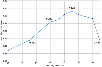
Figure 5: The optimal masking ratio is around 75%. Lower or higher masking ratio will degrade the performance of prediction.

In Table 1, Ti-MAE consistently improves the performance in across all datasets of different prediction horizons. Specifically, Ti-MAE achieves a MAE decrease of 15.7% in ETT, 42.3% in Weather, 45.5% in Exchange and 19.2% in ILI compared to representation learning frameworks. Notably, our Ti-MAE does not require any extra regressor after pre-trained because its decoder can directly generate future time series to be predicted given the input sequence and masking ratio. In Table 2, Ti-MAE ($\dagger$ indicates fine-tuned version) also shows more compatible performance compared to other Transformer-based end-to-end supervised methods. It must be stressed that we have pre-trained only one Ti-MAE model while all the end-to-end supervised models should be trained separately for different settings. Then we just utilize its encoder (parameters have been frozen) with an additional linear projection layer for fine-tuning at different prediction horizons. Runtime analysis comapred to other Transformer-based models could be seen at appendix. To further explore the impact of main properties of Ti-MAE, we conduct extensive ablation experiments on Weather under input sequence length of 200 and prediction horizon of 100 setting for evaluation. Table 3 demonstrates all the results of ablation study.

Table 2: Multivariate time series forecasting results compared to end-to-end methods.

Method		Ti-MAE$\dagger$		ETSformer		FEDformer		Autoformer		Informer
Metric		MSE	MAE	MSE	MAE	MSE	MAE	MSE	MAE	MSE	MAE
ETTh	12	0.2826	0.3383	0.4479	0.4582	0.3272	0.3940	0.5016	0.5204	0.4299	0.4644
	24	0.3430	0.3816	0.4602	0.4621	0.3699	0.4185	0.5063	0.5309	0.4880	0.4963
	48	0.3705	0.3939	0.4855	0.4735	0.3912	0.4347	0.5703	0.5563	0.6625	0.5774
	96	0.4039	0.4074	0.5090	0.4851	0.4194	0.4476	0.6052	0.5663	0.9584	0.7157
	128	0.4270	0.4208	0.5279	0.4949	0.4360	0.4551	0.6043	0.5726	0.9504	0.7197
	168	0.4455	0.4363	0.5446	0.5044	0.4733	0.4783	0.7382	0.6199	1.1043	0.7867
Weather	12	0.0811	0.1199	0.0900	0.1537	0.1476	0.2350	0.2042	0.2960	0.2351	0.3128
	24	0.1065	0.1484	0.1396	0.2224	0.1624	0.2496	0.2200	0.3141	0.1244	0.2022
	48	0.1290	0.1784	0.1848	0.2735	0.1993	0.2898	0.2691	0.3542	0.2352	0.3129
	96	0.1633	0.2151	0.2034	0.2994	0.2350	0.3139	0.2891	0.3673	0.2808	0.3586
	128	0.1774	0.2283	0.2092	0.2972	0.2395	0.3148	0.2758	0.3469	0.3055	0.3723
	168	0.2031	0.2525	0.2199	0.3016	0.2632	0.3281	0.2861	0.3506	0.3473	0.4003
Exchange	24	0.0276	0.1167	0.0266	0.1130	0.0717	0.1958	0.0894	0.2239	0.4963	0.5623
	48	0.0438	0.1481	0.0441	0.1464	0.0954	0.2247	0.1474	0.2881	1.0477	0.8169
	96	0.0814	0.2074	0.0861	0.2044	0.1470	0.2790	0.2883	0.3957	1.1038	0.8215
	128	0.1108	0.2361	0.1153	0.2373	0.1886	0.3153	0.3102	0.4107	1.1978	0.8535
	168	0.1443	0.2824	0.1549	0.2773	0.2484	0.3638	0.3066	0.4108	1.1564	0.8444
	196	0.1661	0.3040	0.1830	0.3034	0.2718	0.3800	0.2990	0.4021	1.1679	0.8545
ILI	24	2.4781	0.9925	3.1358	1.2128	3.3017	1.2689	3.3292	1.2088	4.2526	1.3551
	36	2.2103	0.8956	2.9369	1.1218	2.6125	1.0575	3.4076	1.1688	4.7647	1.4433
	48	1.9697	0.8826	2.9386	1.1120	2.5883	1.0683	3.2077	1.1125	4.8189	1.4553
	60	2.3496	0.9545	2.8840	1.1324	2.8460	1.1533	3.3373	1.1659	4.7974	1.4669
	72	2.1563	0.8884	2.8615	1.1579	2.8921	1.1721	3.1079	1.1237	4.1188	1.3718
	96	2.3860	0.9827	3.1109	1.2186	3.1048	1.2412	3.0530	1.1260	4.5218	1.4401

Masking ratio. Figure 5 and Table 3(a) show the influence of the masking ratio. The optimal ratios are around 75%, which is in contrast to BERT (Devlin et al., 2019) and video-MAE (Feichtenhofer et al., 2022) but similar to MAE for images (He et al., 2021). The high masking ratio induces the model to process fewer tokens and learn high-level semantic information. We can see that lower masking ratios perform worse even if the encoder could see more tokens because the model trained with lower masking ratio may simply recover the values by interpolation or extrapolation, focusing on low level semantic features locally.

Sampling Time Tables 3(b) and 3(c) study the influence of sampling time in each iteration and data augmentation on Ti-MAE training stage. Ti-MAE works well with proper sampling time in each iteration and even no extra data augmentation, which is different from other existing representation learning methods on time series, especially contrastive learning models which rely on heavily data augmentation. Ti-MAE can directly learn adequate information from masked data. Additionally, introducing extra data augmentation will degrade the performance due to inevitable distortions of the original data, which is different from the result of MAE for images or videos. Random masking in each iteration generates a large number of different views without any distortion so that model can make use of visible tokens to capture more useful features.

Table 3: Ablation experiments on Weather. The entries marked in bold are the same which specify the default settings. Lower MSE and MAE represent better performance. This table format follows (Feichtenhofer et al., 2022).

(a) Masking ratio

Ratio	MSE	MAE
0.45	0.3082	0.3557
0.60	0.2650	0.3414
0.75	0.2103	0.2696
0.90	0.2483	0.3176

(b) Sampling time

#Sampling	MSE	MAE
20	0.2151	0.2892
25	0.2447	0.3095
30	0.2103	0.2696
35	0.2171	0.2769

(c) Data augmentation

Case	MSE	MAE
None	0.2103	0.2696
Scaling	0.2383	0.3022
Shifting	0.2399	0.3388
Jittering	0.2508	0.3316

(d) Input sequence length

Length	MSE	MAE
200	0.2413	0.2844
300	0.2103	0.2696
400	0.2877	0.3501
500	0.2328	0.2985

(e) Decoder width

#Blocks	MSE	MAE
1	0.2375	0.2954
2	0.2103	0.2696
3	0.2125	0.3112
4	0.2616	0.3057

(f) Decoder depth

Dim	MSE	MAE
16	0.4374	0.4805
32	0.2103	0.2696
64	0.2380	0.2813
128	0.3172	0.3758

Input sequence length. In Table 3(d) we compare different length of input time series in training stage. Surprisingly, although lengthening the input length of the pre-training stage can improve the performance within limits, too long input sequence may degrade the results of our model because there is a certain conflict between the complex periodic pattern in the long sequence and the short-term prediction task in the downstream.

Decoder Design. Tables 3(e) and 3(f) show the influence of the decoder width and depth. A shallow design of the decoder is sufficient for reconstruction tasks. It is because that time series data are not that complicated and thus need lower decoding dimension to reduce redundancy. Such a lightweight decoder can efficiently reduce computational complexity and memory usage.

4.3 Time Series Classification

In the previous section, we have improved the performance of our framework on forecasting tasks by reducing the consistency between upstream tasks and downstream tasks compared to contrastive learning methods. Thus, we should evaluate learning ability of instance-level representation on classification tasks. The results on 128 UCR archive are summarized in Table 4. Compared to other representation learning methods, Ti-MAE achieves more compatible performance. More details and full results of each dataset in UCR are listed in the appendix. Following (Yue et al., 2022), Critical Difference diagram (Demsar, 2006) for Nemenyi tests conducted on all datasets is shown as Figure 6, where classifiers that are connected by a bold line do not have a significant difference. This proves that Ti-MAE could learn good instance-level representations directly from the raw time series data without any hierarchical tricks or data augmentation.

Table 4: 128 UCR Archive Classification

method	Ti-MAE	TS2Vec	T-Loss	TS-TCC	TST	TNC	DTW
Avg.Acc.	0.8231	0.8201	0.7875	0.7396	0.6385	0.7431	0.7278
Avg.Rank	2.054	3.016	4.016	4.445	4.883	3.875	5.711

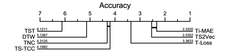
Figure 6: Critical Difference (CD) diagram on UCR classification with a 95% confidence level.

5 Conclusion

This paper proposes a novel self-supervised framework named Ti-MAE for time series representation learning, which randomly masks out tokenized time series and learns an autoencoder to reconstruct them at the point-level. Ti-MAE bridges the connection between contrastive representation learning and generative Transformer-based methods and greatly improves the performance on forecasting tasks due to reducing the inconsistency of upstream and downstream tasks compared to contrastive learning methods. Compared with the fixed continuous masking strategy used in existing Transformer-based models, Ti-MAE adequately leverages all the input sequence and alleviates the distribution shift problem. The flexible setting of masking ratio makes Ti-MAE more adaptive to various prediction scenarios with different time steps. The experiments on real-world datasets and ablation study demonstrate the effectiveness and scalability of our framework. Future work will extend our work for different reconstruction targets according to their requirements.

Appendix A Experimental Details

A.1 Reproduction details for Ti-MAE

The default settings of Ti-MAE are shown in Table 5 in detail. We use one Conv1d layer with the setting of $\text{kernel}=3,\text{stride}=1,\text{padding}=1$ to obtain the encoder input embedding, and then we add a fixed positional encoding as

$$\mathrm{PE}(pos,2i) =\sin(\frac{pos}{10000^{2i/\text{d}_{\text{model}}}})$$ (2)

$$\mathrm{PE}(pos,2i+1) =\cos(\frac{pos}{10000^{2i/\text{d}_{\text{model}}}}),$$

where $\text{d}_{\text{model}}$ represents the number of hidden states. After encoder input embedding, we randomly mask out 75% tokens, and then remaining visible parts are fed into the encoder. The encoder and decoder of Ti-MAE both contain 2 Transformer blocks as widely adopted in  Devlin et al. (2019); Dosovitskiy et al. (2021), each of which consists of one vanilla self-attention layer with 4 heads and a point-wise feed forward layer. As recommended in Dosovitskiy et al. (2021), we adopt pre-norm instead of post-norm for stability of the model in training stage. Equation 3 demonstrates the whole process in the encoder:

$$\mathbf{Z}_{i}^{d} =\mathrm{RandomMask}(\mathrm{Conv1d}(\mathcal{X}_{l,n})+\mathrm{PE}(\mathcal{X}_{l,n}))$$ (3)

$$\hat{\mathbf{Z}_{i}^{d}} =\mathbf{Z}_{i}^{d}+\mathrm{MHSA}(\mathrm{LayerNorm}(\mathbf{Z}_{i}^{d},\mathbf{Z}_{i}^{d},\mathbf{Z}_{i}^{d}))$$

$$\tilde{\mathbf{Z}_{i}^{d}} =\hat{\mathbf{Z}_{i}^{d}}+\mathrm{MLP}(\mathrm{LayerNorm}(\hat{\mathbf{Z}_{i}^{d}}))$$

where we use $\mathcal{X}_{l,n}$ to denote the vectors in dimension $n$ with the length of $l$, and $Z_{i}^{d}$ to denote the intermediate representation in dimension $d$ with the length of $i$. In the decoder, we first apply a linear layer to reduce the input dimension to $d^{\prime}$ ($64\rightarrow 32$) for training efficiency. Given the position to be reconstruct, zero initialized masked tokens are padded to the encoded tokens with the original positional encoding. A dropout layer ($p=0.1$) is added to the bottom of Transformer blocks to prevent the over-fitting problem. The last linear projection layer of the decoder is to reconstruct the missing values at the point-level. Equation 4 demonstrates the whole process of the decoder:

$$\mathbf{Z}_{l}^{d^{\prime}} =\mathrm{Padding}(\mathrm{Linear}(\tilde{\mathbf{Z}_{i}^{d}}))+\mathrm{PE}(\mathcal{X}_{l,d^{\prime}}))$$ (4)

$$\hat{\mathbf{Z}_{l}^{d^{\prime}}} =\mathbf{Z}_{l}^{d^{\prime}}+\mathrm{MHSA}(\mathrm{LayerNorm}(\mathbf{Z}_{l}^{d^{\prime}},\mathbf{Z}_{l}^{d^{\prime}},\mathbf{Z}_{l}^{d^{\prime}}))$$

$$\tilde{\mathbf{Z}_{l}^{d^{\prime}}} =\hat{\mathbf{Z}_{l}^{d^{\prime}}}+\mathrm{MLP}(\mathrm{LayerNorm}(\hat{\mathbf{Z}_{l}^{d^{\prime}}}))$$

$$\tilde{\mathcal{X}_{l,n}} =\mathrm{Projection}(\tilde{\mathbf{Z}_{l}^{d^{\prime}}})$$

where we use $Z_{l}^{d^{\prime}}$ to denote the intermediate representation in dimension $d^{\prime}$ with the length of $l$, and $\tilde{\mathcal{X}_{l,n}}$ to denote our reconstruction goals.

Table 5: Default settings of Ti-MAE

Config	Value
optimizer	Adam Kingma & Ba (2015)
learning rate	0.001
learning rate schedule	cosine decay
epochs	10
masking ratio	75%
sampling time	30
batch size	64
#encoder layer	2
#decoder layer	2
$\text{d}_{\text{model}}$	64
dropout	0.1

Notably, all the linear layers in Ti-MAE are initialized through xavier Glorot & Bengio (2010). The choice of Transformer blocks in Ti-MAE is flexible so that you can use other designed blocks with more inductive biases if necessary.

A.2 Details on baselines

For forecasting tasks, the results of CoST Woo et al. (2022a), TS2Vec Yue et al. (2022), TNC Tonekaboni et al. (2021), MoCo Chen et al. (2021), Autoformer Wu et al. (2021), Informer Zhou et al. (2021), ETSformer Woo et al. (2022b) and FEDformer Zhou et al. (2022) are all based on our reproduction. For classification tasks, the results of TS2Vec are based on our reproduction. Other results of classification are directly taken from Yue et al. (2022).

CoST Woo et al. (2022a) was recently proposed as a contrastive learning framework of disentangled seasonal-trend representations for time series forecasting. They comprises both time domain and frequency domain contrastive losses to learn discriminative trend and seasonal representations. We use the public official source code from https://github.com/salesforce/CoST.

TS2Vec Yue et al. (2022) is a universal framework for learning representations of time series in an arbitrary semantic level through applying contrastive learning in a hierarchical way over augmented context views. TS2Vec can obtain timestamp-level and instance-level representations for forecasting and classification simultaneously. We take the officially implemented code from https://github.com/yuezhihan/ts2vec.

TNC Tonekaboni et al. (2021) is a self-supervised contrastive learning framework for time series, where the positive samples come from the neighboring similar signals. We use the official open source code from https://github.com/sanatonek/TNCrepresentationlearning and all the settings of hyper-parameters follows Woo et al. (2022a).

MoCo Chen et al. (2021) is a self-supervised contrastive learning framework widely used in computer vision domain, which uses a dynamic queue to save a large number of positive and negative samples with consistency. We directly apply this framework on time series data using the official code from https://github.com/facebookresearch/moco. Hyper-parameters are the same as Woo et al. (2022a).

Autoformer Wu et al. (2021) is a novel end-to-end supervised model with a decomposition architecture for time series forecasting. By directly subtracting trend parts obtained from moving average, they design an auto-correlation mechanism as a replacement for self-attention to capture long-term dependencies from seasonality parts. We use their open source code from https://github.com/thuml/Autoformer. Hyper-parameters are remain the default values in the code.

Informer Zhou et al. (2021) is an efficient end-to-end supervised model for time series forecasting. They propose a novel sparse attention to reduce time complexity and memory usage. We take the officially implemented code from https://github.com/zhouhaoyi/Informer2020. Hyper-parameters are used as suggested in their paper.

ETSformer Woo et al. (2022b) proposes an interpretable Transformer architecture which decomposes forecasts into level, growth, and seasonality components. And they employ both exponential smoothing attention and frequency attention to reduce computational complexity. We use their open source code from https://github.com/salesforce/ETSformer. Hyper-parameters are used as suggested in their paper.

FEDformer Zhou et al. (2022) proposes to combine Transformer with the seasonal-trend decomposition method, and exploit the fact that most time series tend to have a sparse representation in well-known basis such as Fourier transform, and develop a frequency enhanced Transformer. We use the official code from https://github.com/MAZiqing/FEDformer. Hyper-parameters are remain the default values in the code.

A.3 Details on benchmark tasks

For time series forecasting tasks, the evaluation settings of end-to-end supervised models and other representation learning methods are slightly different. For other representation learning methods, we follow Yue et al. (2022) to evaluate the performance of their models. Specifically, we use a ridge regression trained on the learned representations to predict the future values. The regularization term $\alpha$ is selected by grid search from $\{0.1,0.2,0.5,1,2,5,10,20,50,100,200,500,1000\}$. It is important to stress that Ti-MAE can directly generate future values from its decoder without any extra regressor (e.g. setting 50% masking ratio means giving one half of the entries to predict the other half.). As for end-to-end models, we set the length of input sequence as 96 to predict future time series with different horizons. Notably, for fair comparison with other SOTA Transformer-based methods including FEDformer and ETSformer on forecasting, we have fine-tuned Ti-MAE on forecasting tasks. Specifically, we extract the encoder of Ti-MAE and freeze it after pre-training, and add an extra linear regressor for fine-tuning.

For classification tasks, we directly obtain instance-level representations by average or max pooling over all timestamps following Yue et al. (2022). To evaluate the performance of models on classification, we follow the same protocol Franceschi et al. (2019), where an SVM classifier with RBF kernel is trained on obtained instance-level representations. The full results of each dataset in UCR are provided in Table 13 and 14.

Notably, due to the flexible design of the Transformer block, we can utilize any layer of the encoder or the decoder of Ti-MAE to get intermediate representations. Extra class token is also a choice if necessary. In our experiments, we simply gather the encoder embedding of Ti-MAE as instance-level representations for evaluation. To accelerate the training of the model, we perform equidistant sampling for different datasets to reduce input to less than 1024 for training efficiency.

Table 6: The classification results on morphological datasets with or without positional encoding

dataset	w/ PE	w/o PE
OSULeaf	0.59	0.74
ShapeletSim	0.54	0.91
Worms	0.64	0.78

TS2Vec also reports an interesting phenomenon that using Transformer instead of Dilated CNN as backbone will largely degrade the performance on classification tasks. We also find similar problems, especially on morphological datasets. We suppose that some morphological datasets have almost no seasonality, while the local morphological characteristics determine the data classification. The positional encoding introduced in the encoder may destroy these morphological features. Simply removing position embedding in the encoder when generating representations will significantly affect the performance of classification. Table 6 shows the classification results on some morphological datasets with or without position embedding.

Appendix B Additional Experimental Results

B.1 The impact of masking ratio and sampling strategies

Table 7: The impact of masking ratio on forecasting tasks.

Method		ETTh		Weather		Excahnge		ILI
Metric		MSE	MAE	MSE	MAE	MSE	MAE	MSE	MAE
Masking	30%	0.6181	0.4984	0.4320	0.4698	0.2707	0.3531	2.2039	0.9908
	45%	0.5140	0.4830	0.3082	0.3557	0.2328	0.3380	2.0452	0.9843
	60%	0.5011	0.4490	0.2650	0.3414	0.2239	0.3340	2.0389	0.9707
	75%	0.4403	0.4338	0.2103	0.2696	0.1701	0.2972	2.0150	0.9646
	90%	0.4597	0.4385	0.2483	0.3176	0.1952	0.3172	2.0332	0.9607

Table 8: The impact of different masking strategies with 75% ratio on Weather.

Masking Strategy	Random	Continuous	Split	Periodic
MSE	0.2103	0.3834	0.3564	0.2720
MAE	0.2696	0.4420	0.3936	0.3357

Table 7 summarizes the impact of masking ratio on different forecasting tasks under the setting of 200-100. We can see that the best masking ratio is generally around 75% given the continuous nature of time series data. Table 8 studies the impact of different masking strategies with 75% ratio on Weather dataset of 96-96 setting. Specifically, random masking means tokens are randomly masked; continuous masking means we only mask historical time series and reconstruct future values, which is the same as traditional forecasting methods; split masking means we both mask historical time series to reconstruct future values, and mask future time series to reconstruct historical sequence; periodic masking means tokens are periodically masked. Notably, periodic masked tokens with a length of four are sampled equidistantly to maintain the same masking ratio. We can see that random masking achieves the best result because randomness can adequately exploit the whole time series data with less inductive bias.

B.2 Running time analysis

Table 9 shows the running time in seconds for each stage of different Transformer-based methods, where we execute three times for each setting (using 96 historical steps to predict future steps of 24, 48, 96, 288 and 672 respectively). All experiments are performed on one single Nvidia V100 GPU. Although many Transformer-based models have $O(L\log L)$ complexity, however, there exists a large constant since these methods generally need to do a bulk of pre-treatment (e.g. Fourier Transform, Wavelet Transform), which makes the overall training not that efficient. In comparison, although our proposed Ti-MAE has $O(L^{2})$ complexity due to the vanilla attention mechanism, we need to pre-train the encoder of Ti-MAE only once and can fine-tune it on different forecasting settings. Thus, the total running time of Ti-MAE is less than other Transformer-based methods.

Table 9: Running time (seconds) for Transformer-based methods at different stages.

Stage	H	Ti-MAE	FEDformer	ETSformer	Autoformer	Informer
Pre-training	/	335.1 $\pm$ 0.5	/	/	/	/
Training	24	17.5 $\pm$ 0.2	170.1 $\pm$ 2.8	68.6 $\pm$ 0.7	61.8 $\pm$ 0.4	68.4 $\pm$ 0.7
	48	17.6 $\pm$ 0.1	199.2 $\pm$ 2.1	69.1 $\pm$ 0.6	68.7 $\pm$ 0.7	76.1 $\pm$ 0.6
	96	17.9 $\pm$ 0.2	250.1 $\pm$ 2.0	72.1 $\pm$ 0.5	79.8 $\pm$ 0.4	87.7 $\pm$ 0.2
	288	18.6 $\pm$ 0.2	324.0 $\pm$ 1.8	73.1 $\pm$ 1.0	130.5 $\pm$ 0.9	137.0 $\pm$ 0.3
	672	19.8 $\pm$ 0.3	460.9 $\pm$ 2.1	76.3 $\pm$ 0.6	220.5 $\pm$ 0.4	220.1 $\pm$ 0.2
Inference	24	5.7 $\pm$ 0.1	9.1 $\pm$ 0.4	9.0 $\pm$ 0.4	13.6 $\pm$ 0.2	9.3 $\pm$ 0.1
	48	6.1 $\pm$ 0.2	10.9 $\pm$ 0.4	9.1 $\pm$ 0.3	15.1 $\pm$ 0.2	10.2 $\pm$ 0.2
	96	6.5 $\pm$ 0.1	12.4 $\pm$ 0.1	9.9 $\pm$ 0.3	18.0 $\pm$ 0.3	12.1 $\pm$ 0.5
	288	8.7 $\pm$ 0.7	16.7 $\pm$ 0.4	13.3 $\pm$ 0.5	31.3 $\pm$ 0.5	18.8 $\pm$ 0.3
	672	12.9 $\pm$ 1.1	25.2 $\pm$ 1.3	19.1 $\pm$ 1.4	55.6 $\pm$ 0.9	31.4 $\pm$ 1.2

B.3 Ablation study on Ti-MAE’s components

Table 10 shows the impact of different components of Ti-MAE, which proves the effectiveness of random masking strategy, Transformer-based backbone and other necessary parts.

Table 10: Ablation study of Ti-MAE’s components on the Exchange dataset (200-100 setting).

Ablation variant	MSE	MAE
Default	0.2111	0.3367
Random $\rightarrow$ fixed continuous masking	0.2505 (-18.7%)	0.3700 (-9.9%)
Encoder w/o positional encoding	0.3082 (-46.0%)	0.3996 (-18.7%)
Decoder w/o positional encoding	0.2276 (-7.8%)	0.3518 (-4.5%)
pre-norm $\rightarrow$ post-norm	0.2213 (-4.8%)	0.3474 (-3.2%)
Transformer $\rightarrow$ TCN	0.2340 (-10.8%)	0.3558 (-5.7%)
Transformer $\rightarrow$ LSTM	0.2406 (-14.0%)	0.3612 (-7.3%)

B.4 Forecasting results with different dimension

The input time series and the output one do not need to have the same dimensionality. Actually the final linear projection layer in the decoder can easily project the input dimensionality to the desired out dimensionality. Table 11 shows the results of using multivariate time series to predict the last univariate target.

Table 11: Forecasting results with different dimension compared to representation learning methods.

Method		Ti-MAE		CoST		TS2Vec		TNC		MoCo
Metric		MSE	MAE	MSE	MAE	MSE	MAE	MSE	MAE	MSE	MAE
ETTh	24	0.031	0.134	0.040	0.152	0.039	0.151	0.057	0.184	0.040	0.151
	48	0.048	0.167	0.060	0.186	0.062	0.189	0.094	0.239	0.063	0.191
	168	0.076	0.207	0.097	0.236	0.142	0.291	0.171	0.329	0.122	0.268
	336	0.097	0.240	0.112	0.306	0.160	0.316	0.192	0.357	0.144	0.297
Weather	24	0.005	0.056	0.096	0.213	0.096	0.215	0.102	0.221	0.097	0.216
	48	0.012	0.087	0.138	0.262	0.140	0.264	0.139	0.264	0.140	0.264
	168	0.014	0.108	0.207	0.334	0.207	0.335	0.198	0.328	0.198	0.326
	336	0.015	0.115	0.230	0.356	0.231	0.360	0.215	0.347	0.220	0.350

B.5 Transferability study

Figure 7: Transferability of Ti-MAE on different trend and seasonality patterns.

To evaluate the transferability of our framework, we generate a set of time series data with different trend and seasonality patterns, which follows

$$y(t)=\cos(\alpha\cdot t)+\cos(\frac{\alpha}{2}\cdot t)+\cos(\frac{\alpha}{4}\cdot t)+\beta\cdot t+\epsilon$$ (5)

where the hyper-parameters $\alpha$ and $\beta$ respectively control the trend and seasonality patterns, and the noises $\epsilon\sim N(0,0.1)$. We train our Ti-MAE under the setting of $\alpha=300,\beta=3$ and evaluate the forecasting performance on other different settings. Table 8 and Figure 7 demonstrate the strong transferability of Ti-MAE under different trend and seasonality patterns.

Table 12: The results of forecasting 400 time steps on simulated time series data with different trend and seasonality patterns.

Setting	$\alpha=300$	$\alpha=600$	$\alpha=300$	$\alpha=600$
	$\beta=3$	$\beta=3$	$\beta=100$	$\beta=100$
MSE	0.0134	0.0596	0.0089	0.0232
MAE	0.0778	0.1912	0.0881	0.0711

Table 13: Full classification results on 128 UCR datasets part 1.

Dataset	TMAE	TS2Vec	T-Loss	TNC	TS-TCC	TST	DTW
ACSF1	0.820	0.870	0.900	0.730	0.730	0.760	0.640
Adiac	0.788	0.726	0.675	0.726	0.767	0.550	0.604
AllGestureWiimoteX	0.633	0.782	0.763	0.703	0.697	0.259	0.716
AllGestureWiimoteY	0.682	0.791	0.726	0.699	0.741	0.423	0.729
AllGestureWiimoteZ	0.671	0.760	0.723	0.646	0.689	0.447	0.643
ArrowHead	0.874	0.794	0.766	0.703	0.737	0.771	0.703
BME	1.000	0.987	0.993	0.973	0.933	0.760	0.900
Beef	0.900	0.700	0.667	0.733	0.600	0.500	0.633
BeetleFly	0.900	0.750	0.800	0.850	0.800	1.000	0.700
BirdChicken	1.000	0.800	0.850	0.750	0.650	0.650	0.750
CBF	1.000	1.000	0.983	0.983	0.998	0.898	0.997
Car	0.867	0.800	0.833	0.683	0.583	0.55	0.733
Chinatown	0.985	0.974	0.951	0.977	0.983	0.936	0.957
ChlorineConcentration	0.725	0.804	0.749	0.760	0.753	0.562	0.648
CinCECGTorso	0.971	0.793	0.713	0.669	0.671	0.508	0.651
Coffee	1.000	1.000	1.000	1.000	1.000	0.821	1.000
Computers	0.780	0.648	0.664	0.684	0.704	0.696	0.700
CricketX	0.674	0.777	0.713	0.623	0.731	0.385	0.754
CricketY	0.659	0.769	0.728	0.597	0.718	0.467	0.744
CricketZ	0.718	0.810	0.708	0.682	0.713	0.403	0.754
Crop	0.751	0.756	0.722	0.738	0.742	0.710	0.665
DiatomSizeReduction	0.984	0.990	0.984	0.993	0.977	0.961	0.967
DistalPhalanxOutlineAgeGroup	0.763	0.719	0.727	0.741	0.755	0.741	0.770
DistalPhalanxOutlineCorrect	0.793	0.754	0.775	0.754	0.754	0.728	0.717
DistalPhalanxTW	0.727	0.698	0.676	0.669	0.676	0.568	0.590
DodgerLoopDay	0.613	0.538	0.241	0.183	0.206	0.200	0.500
DodgerLoopGame	0.739	0.826	0.415	0.508	0.493	0.696	0.877
DodgerLoopWeekend	0.978	0.949	0.623	0.684	0.601	0.732	0.949
ECG200	0.910	0.860	0.940	0.830	0.880	0.830	0.770
ECG5000	0.942	0.932	0.933	0.937	0.941	0.928	0.924
ECGFiveDays	0.988	1.000	1.000	0.999	0.878	0.763	0.768
EOGHorizontalSignal	0.558	0.528	0.605	0.442	0.401	0.373	0.503
EOGVerticalSignal	0.547	0.483	0.434	0.392	0.376	0.298	0.448
Earthquakes	0.748	0.748	0.748	0.748	0.748	0.748	0.719
ElectricDevices	0.685	0.724	0.707	0.700	0.686	0.676	0.602
EthanolLevel	0.744	0.388	0.382	0.424	0.486	0.260	0.276
FaceAll	0.880	0.789	0.786	0.766	0.813	0.504	0.808
FaceFour	0.875	0.852	0.920	0.659	0.773	0.511	0.830
FacesUCR	0.866	0.929	0.884	0.789	0.863	0.543	0.905
FiftyWords	0.787	0.754	0.732	0.653	0.653	0.525	0.690
Fish	0.897	0.920	0.891	0.817	0.817	0.720	0.823
FordA	0.818	0.940	0.928	0.902	0.930	0.568	0.555
FordB	0.652	0.802	0.793	0.733	0.815	0.507	0.620
FreezerRegularTrain	0.987	0.984	0.956	0.991	0.989	0.922	0.899
FreezerSmallTrain	0.959	0.872	0.933	0.982	0.979	0.920	0.753
Fungi	0.968	0.935	1.000	0.527	0.753	0.366	0.839
GestureMidAirD1	0.662	0.592	0.608	0.431	0.369	0.208	0.569
GestureMidAirD2	0.546	0.523	0.546	0.362	0.254	0.138	0.608
GestureMidAirD3	0.400	0.323	0.285	0.292	0.177	0.154	0.323
GesturePebbleZ1	0.901	0.849	0.919	0.378	0.395	0.500	0.791
GesturePebbleZ2	0.918	0.854	0.899	0.316	0.430	0.380	0.671
GunPoint	0.993	0.973	0.980	0.967	0.993	0.827	0.907
GunPointAgeSpan	0.994	0.962	0.994	0.984	0.994	0.991	0.918
GunPointMaleVersusFemale	0.997	1.000	0.997	0.994	0.997	1.000	0.997
GunPointOldVersusYoung	1.000	1.000	1.000	1.000	1.000	1.000	0.838
Ham	0.800	0.714	0.724	0.752	0.743	0.524	0.467
HandOutlines	0.919	0.919	0.922	0.930	0.724	0.735	0.881
Haptics	0.484	0.519	0.490	0.474	0.396	0.357	0.377
Herring	0.656	0.609	0.594	0.594	0.594	0.594	0.531
HouseTwenty	0.941	0.899	0.933	0.782	0.790	0.815	0.924
InlineSkate	0.380	0.403	0.371	0.378	0.347	0.287	0.384
InsectEPGRegularTrain	1.000	1.000	1.000	1.000	1.000	1.000	0.872
InsectEPGSmallTrain	1.000	1.000	1.000	1.000	1.000	1.000	0.735
InsectWingbeatSound	0.639	0.616	0.597	0.549	0.415	0.266	0.355

Table 14: Full classification results on 128 UCR datasets part 2.

Dataset	TMAE	TS2Vec	T-Loss	TNC	TS-TCC	TST	DTW
ItalyPowerDemand	0.967	0.932	0.954	0.928	0.955	0.845	0.950
LargeKitchenAppliances	0.787	0.869	0.789	0.776	0.848	0.595	0.795
Lightning2	0.836	0.869	0.869	0.869	0.836	0.705	0.869
Lightning7	0.808	0.781	0.795	0.767	0.685	0.411	0.726
Mallat	0.956	0.904	0.951	0.871	0.922	0.713	0.934
Meat	0.967	0.967	0.950	0.917	0.883	0.900	0.933
MedicalImages	0.771	0.799	0.750	0.754	0.747	0.632	0.737
MelbournePedestrian	0.949	0.958	0.944	0.942	0.949	0.741	0.791
MiddlePhalanxOutlineAgeGroup	0.675	0.643	0.656	0.643	0.630	0.617	0.500
MiddlePhalanxOutlineCorrect	0.811	0.831	0.825	0.818	0.818	0.753	0.698
MiddlePhalanxTW	0.623	0.578	0.591	0.571	0.610	0.506	0.506
MixedShapesRegularTrain	0.922	0.917	0.905	0.911	0.855	0.879	0.842
MixedShapesSmallTrain	0.875	0.854	0.860	0.813	0.735	0.828	0.780
MoteStrain	0.913	0.859	0.851	0.825	0.843	0.768	0.835
NonInvasiveFetalECGThorax1	0.918	0.924	0.878	0.898	0.898	0.471	0.790
NonInvasiveFetalECGThorax2	0.938	0.939	0.919	0.912	0.913	0.832	0.865
OSULeaf	0.736	0.851	0.760	0.723	0.723	0.545	0.591
OliveOil	0.933	0.867	0.867	0.833	0.800	0.800	0.833
PLAID	0.458	0.555	0.555	0.495	0.445	0.419	0.840
PhalangesOutlinesCorrect	0.772	0.806	0.784	0.787	0.804	0.773	0.728
Phoneme	0.229	0.296	0.276	0.180	0.242	0.139	0.228
PickupGestureWiimoteZ	0.840	0.800	0.740	0.620	0.600	0.240	0.660
PigAirwayPressure	0.240	0.807	0.510	0.413	0.380	0.120	0.106
PigArtPressure	0.760	0.966	0.928	0.808	0.524	0.774	0.245
PigCVP	0.750	0.813	0.788	0.649	0.615	0.596	0.154
Plane	1.000	0.990	0.990	1.000	1.000	0.933	1.000
PowerCons	1.000	0.967	0.900	0.933	0.961	0.911	0.878
ProximalPhalanxOutlineAgeGroup	0.863	0.834	0.844	0.854	0.839	0.854	0.805
ProximalPhalanxOutlineCorrect	0.876	0.890	0.859	0.866	0.873	0.770	0.784
ProximalPhalanxTW	0.829	0.790	0.771	0.810	0.800	0.780	0.761
RefrigerationDevices	0.611	0.603	0.515	0.565	0.563	0.483	0.464
Rock	0.660	0.660	0.580	0.580	0.600	0.680	0.600
ScreenType	0.579	0.411	0.416	0.509	0.419	0.419	0.397
SemgHandGenderCh2	0.838	0.960	0.890	0.882	0.837	0.725	0.802
SemgHandMovementCh2	0.700	0.862	0.789	0.593	0.613	0.420	0.584
SemgHandSubjectCh2	0.813	0.947	0.853	0.771	0.753	0.484	0.727
ShakeGestureWiimoteZ	0.900	0.940	0.920	0.820	0.860	0.760	0.860
ShapeletSim	0.911	0.939	0.672	0.589	0.683	0.489	0.650
ShapesAll	0.840	0.890	0.848	0.788	0.773	0.733	0.768
SmallKitchenAppliances	0.741	0.733	0.677	0.725	0.691	0.592	0.643
SmoothSubspace	0.993	0.980	0.960	0.913	0.953	0.827	0.827
SonyAIBORobotSurface1	0.912	0.910	0.902	0.804	0.899	0.724	0.725
SonyAIBORobotSurface2	0.934	0.897	0.889	0.834	0.907	0.745	0.831
StarLightCurves	0.972	0.971	0.964	0.968	0.967	0.949	0.907
Strawberry	0.970	0.967	0.954	0.951	0.965	0.916	0.941
SwedishLeaf	0.938	0.923	0.914	0.880	0.923	0.738	0.792
Symbols	0.961	0.981	0.963	0.885	0.916	0.786	0.950
SyntheticControl	0.993	0.997	0.987	1.000	0.990	0.490	0.993
ToeSegmentation1	0.890	0.925	0.939	0.864	0.930	0.807	0.772
ToeSegmentation2	0.908	0.900	0.900	0.831	0.877	0.615	0.838
Trace	1.000	1.000	0.990	1.000	1.000	1.000	1.000
TwoLeadECG	0.985	0.982	0.999	0.993	0.976	0.871	0.905
TwoPatterns	0.994	1.000	0.999	1.000	0.999	0.466	1.000
UMD	1.000	0.993	0.993	0.993	0.986	0.910	0.993
UWaveGestureLibraryAll	0.956	0.938	0.896	0.903	0.692	0.475	0.892
UWaveGestureLibraryX	0.814	0.797	0.785	0.781	0.733	0.569	0.728
UWaveGestureLibraryY	0.736	0.714	0.710	0.697	0.641	0.348	0.634
UWaveGestureLibraryZ	0.749	0.759	0.757	0.721	0.690	0.655	0.658
Wafer	0.996	0.999	0.992	0.994	0.994	0.991	0.980
Wine	0.907	0.741	0.815	0.759	0.778	0.500	0.574
WordSynonyms	0.705	0.676	0.691	0.630	0.531	0.422	0.649
Worms	0.779	0.727	0.727	0.623	0.753	0.455	0.584
WormsTwoClass	0.792	0.740	0.792	0.727	0.753	0.584	0.623
Yoga	0.834	0.888	0.837	0.812	0.791	0.830	0.837

References

- Bao et al. (2021) Hangbo Bao, Li Dong, and Furu Wei. Beit: Bert pre-training of image transformers. ArXiv, abs/2106.08254, 2021.
- Carbonneau et al. (2008) Réal André Carbonneau, Kevin Laframboise, and Rustam M. Vahidov. Application of machine learning techniques for supply chain demand forecasting. Eur. J. Oper. Res., 184:1140–1154, 2008.
- Chen et al. (2021) Xinlei Chen, Saining Xie, and Kaiming He. An empirical study of training self-supervised vision transformers. 2021 IEEE/CVF International Conference on Computer Vision (ICCV), pp. 9620–9629, 2021.
- Chen et al. (2013) Yanping Chen, Bing Hu, Eamonn J. Keogh, and Gustavo E. A. P. A. Batista. Dtw-d: time series semi-supervised learning from a single example. Proceedings of the 19th ACM SIGKDD international conference on Knowledge discovery and data mining, 2013.
- Child et al. (2019) Rewon Child, Scott Gray, Alec Radford, and Ilya Sutskever. Generating long sequences with sparse transformers. ArXiv, abs/1904.10509, 2019.
- Dau et al. (2019) Hoang Anh Dau, A. Bagnall, Kaveh Kamgar, Chin-Chia Michael Yeh, Yan Zhu, Shaghayegh Gharghabi, Chotirat Ratanamahatana, and Eamonn J. Keogh. The ucr time series archive. IEEE/CAA Journal of Automatica Sinica, 6:1293–1305, 2019.
- Demsar (2006) Janez Demsar. Statistical comparisons of classifiers over multiple data sets. J. Mach. Learn. Res., 7:1–30, 2006.
- Devlin et al. (2019) Jacob Devlin, Ming-Wei Chang, Kenton Lee, and Kristina Toutanova. Bert: Pre-training of deep bidirectional transformers for language understanding. ArXiv, abs/1810.04805, 2019.
- Dosovitskiy et al. (2021) Alexey Dosovitskiy, Lucas Beyer, Alexander Kolesnikov, Dirk Weissenborn, Xiaohua Zhai, Thomas Unterthiner, Mostafa Dehghani, Matthias Minderer, Georg Heigold, Sylvain Gelly, Jakob Uszkoreit, and Neil Houlsby. An image is worth 16x16 words: Transformers for image recognition at scale. ArXiv, abs/2010.11929, 2021.
- Eldele et al. (2021) Emadeldeen Eldele, Mohamed Ragab, Zhenghua Chen, Min Wu, C. Kwoh, Xiaoli Li, and Cuntai Guan. Time-series representation learning via temporal and contextual contrasting. ArXiv, abs/2106.14112, 2021.
- fang Zha (2022) Meng fang Zha. Time series generation with masked autoencoder. ArXiv, abs/2201.07006, 2022.
- Feichtenhofer et al. (2022) Christoph Feichtenhofer, Haoqi Fan, Yanghao Li, and Kaiming He. Masked autoencoders as spatiotemporal learners. ArXiv, abs/2205.09113, 2022.
- Franceschi et al. (2019) Jean-Yves Franceschi, Aymeric Dieuleveut, and Martin Jaggi. Unsupervised scalable representation learning for multivariate time series. In NeurIPS, 2019.
- Glorot & Bengio (2010) Xavier Glorot and Yoshua Bengio. Understanding the difficulty of training deep feedforward neural networks. In AISTATS, 2010.
- He et al. (2021) Kaiming He, Xinlei Chen, Saining Xie, Yanghao Li, Piotr Doll’ar, and Ross B. Girshick. Masked autoencoders are scalable vision learners. ArXiv, abs/2111.06377, 2021.
- Hou et al. (2022) Zhenyu Hou, Xiao Liu, Yukuo Cen, Yuxiao Dong, Hongxia Yang, Chun-Wei Wang, and Jie Tang. Graphmae: Self-supervised masked graph autoencoders. ArXiv, abs/2205.10803, 2022.
- Kingma & Ba (2015) Diederik P. Kingma and Jimmy Ba. Adam: A method for stochastic optimization. CoRR, abs/1412.6980, 2015.
- Lai et al. (2018) Guokun Lai, Wei-Cheng Chang, Yiming Yang, and Hanxiao Liu. Modeling long- and short-term temporal patterns with deep neural networks. The 41st International ACM SIGIR Conference on Research & Development in Information Retrieval, 2018.
- Laptev et al. (2017) Nikolay Pavlovich Laptev, Jason Yosinski, Li Erran Li, and Slawek Smyl. Time-series extreme event forecasting with neural networks at uber. 2017.
- Lei et al. (2019) Qi Lei, Jinfeng Yi, Roman Vaculín, Lingfei Wu, and Inderjit S. Dhillon. Similarity preserving representation learning for time series clustering. In IJCAI, 2019.
- LI et al. (2019) SHIYANG LI, Xiaoyong Jin, Yao Xuan, Xiyou Zhou, Wenhu Chen, Yu-Xiang Wang, and Xifeng Yan. Enhancing the locality and breaking the memory bottleneck of transformer on time series forecasting. ArXiv, abs/1907.00235, 2019.
- Liu et al. (2022) Shizhan Liu, Hang Yu, Cong Liao, Jianguo Li, Weiyao Lin, Alex X. Liu, and Schahram Dustdar. Pyraformer: Low-complexity pyramidal attention for long-range time series modeling and forecasting. In International Conference on Learning Representations, 2022. URL https://openreview.net/forum?id=0EXmFzUn5I.
- Ma et al. (2019) Jiawei Ma, Zheng Shou, Alireza Zareian, Hassan Mansour, Anthony Vetro, and Shih-Fu Chang. Cdsa: Cross-dimensional self-attention for multivariate, geo-tagged time series imputation. ArXiv, abs/1905.09904, 2019.
- Oreshkin et al. (2020) Boris N. Oreshkin, Dmitri Carpov, Nicolas Chapados, and Yoshua Bengio. N-beats: Neural basis expansion analysis for interpretable time series forecasting. ArXiv, abs/1905.10437, 2020.
- Pang et al. (2022) Yatian Pang, Wenxiao Wang, Francis E. H. Tay, W. Liu, Yonghong Tian, and Liuliang Yuan. Masked autoencoders for point cloud self-supervised learning. ArXiv, abs/2203.06604, 2022.
- Paszke et al. (2019) Adam Paszke, Sam Gross, Francisco Massa, Adam Lerer, James Bradbury, Gregory Chanan, Trevor Killeen, Zeming Lin, Natalia Gimelshein, Luca Antiga, Alban Desmaison, Andreas Köpf, Edward Yang, Zach DeVito, Martin Raison, Alykhan Tejani, Sasank Chilamkurthy, Benoit Steiner, Lu Fang, Junjie Bai, and Soumith Chintala. Pytorch: An imperative style, high-performance deep learning library. In NeurIPS, 2019.
- Pathak et al. (2016) Deepak Pathak, Philipp Krähenbühl, Jeff Donahue, Trevor Darrell, and Alexei A. Efros. Context encoders: Feature learning by inpainting. 2016 IEEE Conference on Computer Vision and Pattern Recognition (CVPR), pp. 2536–2544, 2016.
- Qiu et al. (2018) Jinwen Qiu, Sreenivasa Rao Jammalamadaka, and Ning Ning. Multivariate bayesian structural time series model. J. Mach. Learn. Res., 19:68:1–68:33, 2018.
- Shao et al. (2022) Zezhi Shao, Zhao Zhang, Fei Wang, and Yongjun Xu. Pre-training enhanced spatial-temporal graph neural network for multivariate time series forecasting. In Proceedings of the 28th ACM SIGKDD Conference on Knowledge Discovery and Data Mining, KDD ’22, pp. 1567–1577, New York, NY, USA, 2022. Association for Computing Machinery. ISBN 9781450393850. doi: 10.1145/3534678.3539396. URL https://doi.org/10.1145/3534678.3539396.
- Song et al. (2018) Huan-Zhi Song, Deepta Rajan, Jayaraman J. Thiagarajan, and Andreas Spanias. Attend and diagnose: Clinical time series analysis using attention models. In AAAI, 2018.
- Tonekaboni et al. (2021) Sana Tonekaboni, Danny Eytan, and Anna Goldenberg. Unsupervised representation learning for time series with temporal neighborhood coding. ArXiv, abs/2106.00750, 2021.
- Tong et al. (2022) Zhan Tong, Yibing Song, Jue Wang, and Limin Wang. Videomae: Masked autoencoders are data-efficient learners for self-supervised video pre-training. ArXiv, abs/2203.12602, 2022.
- van den Oord et al. (2018) Aäron van den Oord, Yazhe Li, and Oriol Vinyals. Representation learning with contrastive predictive coding. ArXiv, abs/1807.03748, 2018.
- Vaswani et al. (2017) Ashish Vaswani, Noam M. Shazeer, Niki Parmar, Jakob Uszkoreit, Llion Jones, Aidan N. Gomez, Lukasz Kaiser, and Illia Polosukhin. Attention is all you need. ArXiv, abs/1706.03762, 2017.
- Vincent et al. (2008) Pascal Vincent, H. Larochelle, Yoshua Bengio, and Pierre-Antoine Manzagol. Extracting and composing robust features with denoising autoencoders. In ICML ’08, 2008.
- Woo et al. (2022a) Gerald Woo, Chenghao Liu, Doyen Sahoo, Akshat Kumar, and Steven Hoi. CoST: Contrastive learning of disentangled seasonal-trend representations for time series forecasting. In International Conference on Learning Representations, 2022a. URL https://openreview.net/forum?id=PilZY3omXV2.
- Woo et al. (2022b) Gerald Woo, Chenghao Liu, Doyen Sahoo, Akshat Kumar, and Steven C. H. Hoi. Etsformer: Exponential smoothing transformers for time-series forecasting. ArXiv, abs/2202.01381, 2022b.
- Wu et al. (2021) Haixu Wu, Jiehui Xu, Jianmin Wang, and Mingsheng Long. Autoformer: Decomposition transformers with auto-correlation for long-term series forecasting. In NeurIPS, 2021.
- Yue et al. (2022) Zhihan Yue, Yujing Wang, Juanyong Duan, Tianmeng Yang, Congrui Huang, Yu Tong, and Bixiong Xu. Ts2vec: Towards universal representation of time series. In AAAI, 2022.
- Zerveas et al. (2021) George Zerveas, Srideepika Jayaraman, Dhaval Patel, Anuradha Bhamidipaty, and Carsten Eickhoff. A transformer-based framework for multivariate time series representation learning. Proceedings of the 27th ACM SIGKDD Conference on Knowledge Discovery & Data Mining, 2021.
- Zhang et al. (2017) Richard Zhang, Phillip Isola, and Alexei A. Efros. Split-brain autoencoders: Unsupervised learning by cross-channel prediction. 2017 IEEE Conference on Computer Vision and Pattern Recognition (CVPR), pp. 645–654, 2017.
- Zhou et al. (2021) Haoyi Zhou, Shanghang Zhang, Jieqi Peng, Shuai Zhang, Jianxin Li, Hui Xiong, and Wan Zhang. Informer: Beyond efficient transformer for long sequence time-series forecasting. In AAAI, 2021.
- Zhou et al. (2022) Tian Zhou, Ziqing Ma, Qingsong Wen, Xue Wang, Liang Sun, and Rong Jin. Fedformer: Frequency enhanced decomposed transformer for long-term series forecasting. In ICML, 2022.